Universal temporal features of rankings in competitive sports and games

Abstract

Many complex phenomena, from the selection of traits in biological systems to hierarchy formation in social and economic entities, show signs of competition and heterogeneous performance in the temporal evolution of their components, which may eventually lead to stratified structures such as the wealth distribution worldwide. However, it is still unclear whether the road to hierarchical complexity is determined by the particularities of each phenomena, or if there are universal mechanisms of stratification common to many systems. Human sports and games, with their (varied but simplified) rules of competition and measures of performance, serve as an ideal test bed to look for universal features of hierarchy formation. With this goal in mind, we analyse here the behaviour of players and team rankings over time for several sports and games. Even though, for a given time, the distribution of performance ranks varies across activities, we find statistical regularities in the dynamics of ranks. Specifically the rank diversity, a measure of the number of elements occupying a given rank over a length of time, has the same functional form in sports and games as in languages, another system where competition is determined by the use or disuse of grammatical structures. Our results support the notion that hierarchical phenomena may be driven by the same underlying mechanisms of rank formation, regardless of the nature of their components. Moreover, such regularities can in principle be used to predict lifetimes of rank occupancy, thus increasing our ability to forecast stratification in the presence of competition.

Research

1 Introduction

Sports and games can be described as complex systems due to the myriad of factors influencing the dynamics of competition and performance in them, including networked interactions among players, human and environmental heterogeneities, and other traits at the individual and group levels [1, 2, 3, 4]. In particular, player performance is influenced by a variety of causes: Economical, political and geographical conditions determine the ranking of a single player and thus may be used for predicting performance. Moreover, the (relatively) simple rules of competition and measures of performance associated with sports and games allow us to explore basic mechanisms of interaction leading to hierarchy formation that may be common to many systems driven by competition, not only leisure activities but other social, biological and economic systems. With this goal in mind, the availability of a large corpus of data related to sports, teams, and players allows researchers to perform multiple statistical analyses, in particular with respect to the structure and dynamics of player rankings [5, 6, 7].

Data availability has made it possible not only to study the distribution of scores determining rankings, but also its time evolution [8]. In a recent paper, Deng et al. present a statistical analysis of 12 sports showing a universal scaling in rankings, despite the fact that the sports considered have very different ranking systems [9]. Here, we focus on the temporal trajectories of player and team performances, meaning the evolution of rank, with the objective of finding statistical regularities that indicate how competition shapes hierarchies of players and teams. In general, rankings are affected in time by events as apparently insignificant as a bad breakfast prior to an important event, or the weather during a competition [10]. Since these factors are inherently present for all activities, we would expect the evolution of rank to have universal features across sports and games.

We propose to quantify such evolution by means of a recently introduced measure, the rank diversity. With the help of the Google $n$-gram dataset [11], rank diversity has been used before to study how vocabulary changes in time [12]. That work shows that rank diversity has the same functional form for all languages studied, and is able to discriminate the size of the core of each language. Thus, we concentrate on the temporal features of rank distributions corresponding to several sports and games with different ranking schemes. We consider data where an appropriate time resolution is available, and limit the analysis to six activities only: tennis, chess, golf, poker and football (national teams and clubs). We find that all rank diversities have the same functional form as languages, despite having very different rank frequency distributions. Finally, we introduce a random walker model that, tuned by the parameter values of each dataset, reproduces qualitatively the diversity of all sports and games considered.

The article is organized as follows. In section Section 2 we describe the datasets used. We then analyse ranking distributions in Section 3 and compare them with several models. Finally, in Section 4 we study the rank diversity for each sport and compare it with the random walker model. The main conclusions of our analysis are stated in Section 5.

2 Ranking data

We use ranking data on players and teams from six sports and games: a) Tennis players (male), ranked by the Association of Tennis Professionals (ATP) [13]; b) Chess players (male), ranked by the Fédération Internationale des Échecs (FIDE) [14]; c) Golf players, ranked by the Official World Golf Ranking (OWGR) [15]; d) Poker players, ranked by the Global Poker Index (GPI) [16]; e) Football teams, ranked by the Football Club World Ranking (FCWR) [17]; and f) national football teams, ranked by the Fédération Internationale de Football Association (FIFA) [18].

The ranking procedure varies among sports. In ATP, for example, tennis players are ordered according to the number of points they have up to the date of publication of the ranking. The number of points depends on the tournaments players have participated in (and how well they have performed), but not all tournaments are taken into account. FIDE uses the Elo system [19] to rank players, which considers the number of matches, their results, and the opponent ranking. The FIFA ranking takes into account official matches between countries. The number of points depends on the confederation and classification of each team, as well as the importance and result of the match. Table 1 summarizes the main properties of the ranking data used in this study, including the temporal resolution of rankings. In order to have a homogeneous ranking resolution for each sport, we disregard some data for the ATP, FIDE, and GPI datasets. In poker, for example, due to the characteristics of some tournaments, rankings for periods shorter than a week may exist, yet we only use weekly data.

3 Comparison with ranking models

Player or team performance is usually measured by a score that varies with time. This score results in a time-dependent rank with rather complex behaviour, as we will explain below. We first focus on the distribution of scores versus ranks (i.e. a rank distribution) for a given time. Particularly, we are interested in seeing if this distribution can be reproduced by a single ranking model for all sports and games considered. We select five ranking models to fit the data, four of which are particular cases of

$$f(k)=\mathcal{N}\frac{(N+1-k)^{d}\exp(-bk)}{k^{a}},$$ (1)

where $f$ is the score associated with rank $k$, $a$ is an exponent that dominates most of the curve, $b$ an exponent controlling its exponential decay, and $d$ an algebraic decay that regulates a sharp drop of the curve for its last elements. Finally, $N$ is the total number of elements (i.e. players or teams) in the system, and $\mathcal{N}$ is a normalization constant.

The first four models are

$$m_{1}(k)\propto\frac{1}{k^{a}},\quad m_{2}(k)\propto\frac{\exp(-bk)}{k^{a}},\quad m_{3}(k)\propto\frac{(N+1-k)^{d}}{k^{a}},\quad m_{4}(k)=f(k),$$ (2)

whereas the fifth model is a double Zipf law [20],

$$m_{5}(k)=\mathcal{N}\begin{cases}\frac{1}{k^{a}}&k\leq k_{c}\\ \frac{k_{c}^{a^{\prime}-a}}{k^{a^{\prime}}}&k>k_{c}\end{cases},$$ (3)

with $a^{\prime}$ an alternative exponent that regulates the behaviour of the curve after a critical rank $k_{c}$. Model $m_{1}$ is obtained by setting $d=b=0$ in Eq. (1), and has been considered in a vast amount of studies, both in the realm of sports [21, 22] and in other studies of ranking behaviour [23], including the famous Zipf’s law of languages where the particular case $a=1$ has drawn a lot of attention (see, e.g., [24] and references therein). The Gamma ($m_{2}$) and Beta ($m_{3}$) distributions have been useful in many disciplines for decades; a quick look at their Wikipedia entries provides numerous examples [25, 26]. Model $m_{4}$, being a more general expression than the previous ones, tends to provide a better fit at the expense of more parameters, and will serve as benchmark for the comparison between the rest of the models. Finally, model $m_{5}$ in Eq. (3) has been used with success in several contexts [20, 27], prompting us to test it in the area of sports and games.

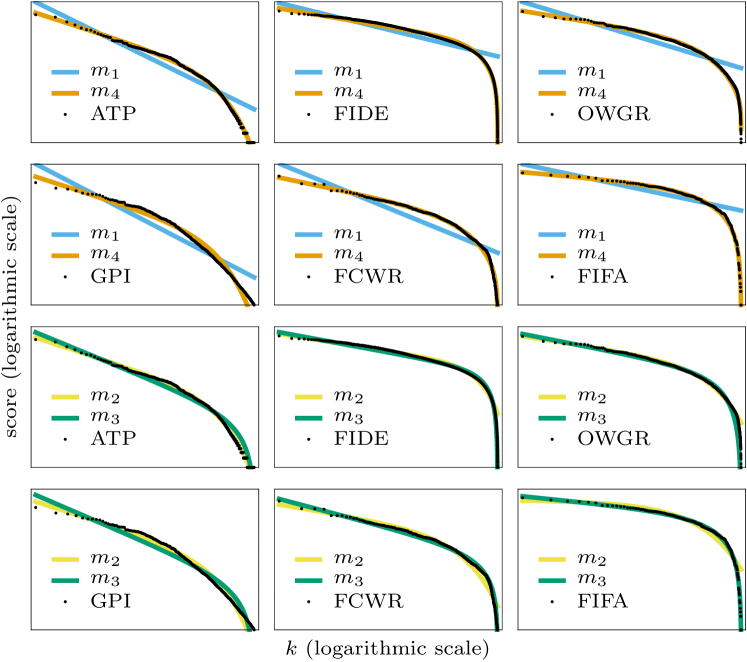
The results of the fitting process between data and Eqs. (1)-(3) are shown in Fig. 1, while Table 2 summarises the parameter values obtained. Data corresponds to a single time snapshot for all sports and games: Sept 25 2014 (ATP); Sept 2014 (FIDE); Mar 18 2015 (GPI); Apr 19, 2015 (OWGR); Dec 29 2014 (FCWR); and Dec 18 2014 (FIFA). Both models and sports show variation in their goodness of fit. From Fig. 1 it is clear that Zipf’s law ($m_{1}$) is not adequate. On the other hand, the Gamma distribution ($m_{2}$) fits some datasets rather well, particularly those that do not show an abrupt fall of score as a function of rank (ATP and GPI). Datasets with an abrupt decay of frequency are well fitted by the Beta distribution ($m_{3}$) (FIDE, OWGR, and FIFA). FCWR is an intermediate case where both functions seem to capture global behaviour accurately, and thus the fit is considerably better for a combination of both models, i.e. $m_{4}$. We also see that the double Zipf law ($m_{5}$) is a good fit for GPI, as seen from Table 3.

In order to objectively compare goodness of fit between models, we consider several measures: The least-squares parameter $R^{2}$, the maximum deviation between theory and observation $D$, and the Kolmogorov index $p$ [28]. $R^{2}$ is calculated as the 2-norm with respect to the data, that is, $R^{2}=\sum_{k}[m_{i}(k)-y_{k})]^{2}$ for a given model fit $m_{i}(k)$, $i=1,\ldots,5$, and data $y_{k}$. The closer $R^{2}$ is to one, the better the fit is. To calculate $D$, we consider the cumulative of both the proposed distribution [here, $m_{i}(k)$] and the dataset with $N$ data points. For a given model $m_{i}(k)$, the cumulative is simply $M_{i}(k)=\int_{-\infty}^{k}m_{i}(\kappa)d\kappa$, whereas for a dataset, $M_{\rm data}(k)=(1/N)\sum_{i}\theta(k-k_{i})$, with $\theta$ a step function [29]. We then define $D$ as the maximum vertical difference between the two curves, that is, $D=\max_{k}|M_{i}(k)-M_{\rm data}(k)|$. The Kolmogorov index $p$ is calculated as follows: Consider the value of $D$ for a given dataset. We then generate the same number of points $N$ using the proposed model, say $m_{i}$, and repeat the procedure to obtain a new $\tilde{D}$. We repeat several times to obtain a set of $\tilde{D}$ values (in our case, 2500). The index $p$ is the fraction of synthetic datasets that have larger $D$ than the original dataset analysed. The measure $p$ allows us to consider that a small dataset will have some noise due to poor statistics. Thus, if a model is consistent with a dataset, but we have poor statistics, we might still have a good (large) $p$. Usually, a “good” fit is required to have $p>0.1$, see e.g. [30].

Table 3 summarises the values of $R^{2}$, $D$, and $p$ found for the six sports and five models $m_{i}$. None of the models are a good fit for all sports, although $m_{4}$ is the most appropriate in terms of $R^{2}$ for most sports. The exception is OWGR, where $m_{5}$ fits slightly better. However, in three cases (FIDE, GPI, and FCWR) we have $p=0$ for model $m_{4}$, and no model fits well, meaning that the theoretical distribution is not followed by the data. For the other three sports (OWGR, FIFA, and ATP), $m_{2}$, $m_{3}$, and $m_{4}$, respectively, are the best fit. At least with the data and models considered, we find no signs of universality. We stress again that Zipf’s law ($m_{1}$) is the worst fit among all considered. It is interesting to notice that $R^{2}$ and $p$ lead to different criteria of what is a ‘good’ or ‘bad’ model. This is due to both the amount of available data and the number of parameters in the model. The larger the data, the easier it is to distinguish an appropriate model from a good (but not accurate enough) approximation. On the other hand, the more parameters the model has, the easier it is to fit any data. Both of these aspects are taken into account in the definition of $p$, but not in $R^{2}$.

4 Rank diversity in sports

In this paper we contribute to the analysis of sports ranking by computing the rank diversity, a measure of the number of elements occupying a given rank over a length of time. It appears that rank diversity has the same functional form, not only for sports but also for other complex systems, such as countries classified by their economic complexity, the 500 leading enterprises ranked by the Fortune magazine, or a set of millions of words in six Indo-European languages [12].

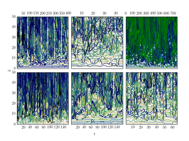
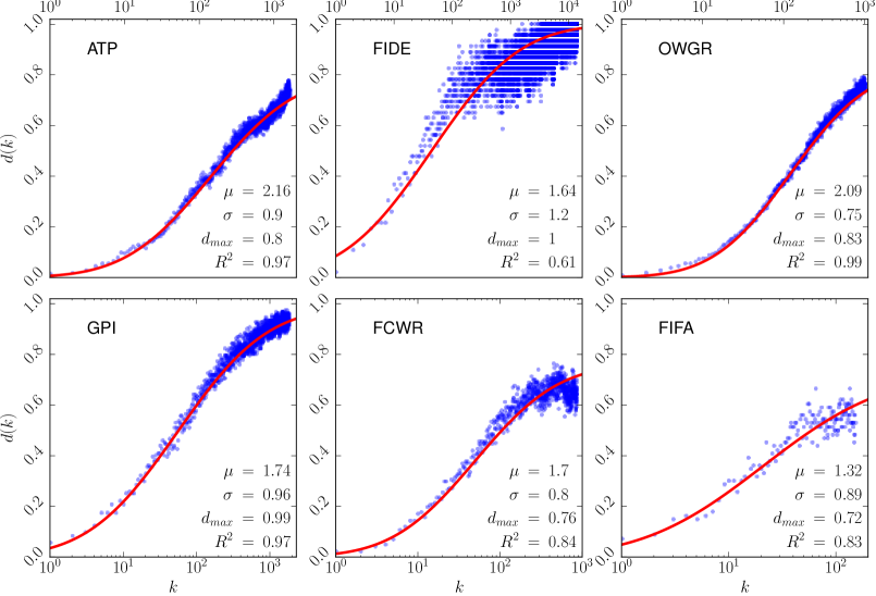
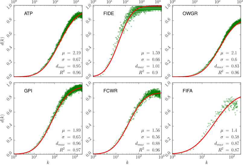
The rank diversity $d(k)$ is defined as the number of distinct elements in a complex system that occupy the rank $k$ at some point during a given length of time. In other words, we choose to focus on the time dependence of ranks, rather than on a static distribution such as $f(k)$. An example of the change of ranks in time for the sports and games studied here can be seen in Fig. 2. These so-called “spaghetti” curves show how elements—individuals or teams—change their rank in time. The rank diversity $d(k)$ is simply the normalized number of different elements (curves) that spend at least one time interval at a given rank $k$. The rank diversity for the various sports and games is shown in Fig. 3.

Studying $d(k)$ for six Indo-European languages [12], we found that the observed rank diversity closely follows the cumulative of a Gaussian (i.e. a sigmoid)

$$\Phi_{\mu,\sigma}(\log k)=\frac{\max_{i}d(k_{i})}{\sigma\sqrt{2\pi}}\int_{-\infty}^{\log k}\exp\left(-\frac{(y-\mu)^{2}}{2\sigma^{2}}\right){\rm d}y.$$ (4)

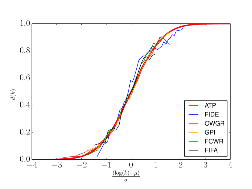
The mean value $\mu$ is set as the smallest $k_{0}$ for which $d(k_{0})=\frac{\max_{i}d(k_{i})}{2}$, while the width $\sigma$ is fitted and gives the scale for which $d(k)$ gets close to its extreme values. If $k_{\pm}$ are given by $\log_{10}k_{\pm}=\mu\pm 2\sigma$, the bulk of the changes in the values of diversity lies between $k_{-}$ and $k_{+}$. In Fig. 3 we show the fit $\Phi$ for all sports and games considered here ($R^{2}$ values for the $\Phi$ curves are shown there as well). We do not consider neither $D$ nor $p$, since these measures are only meaningful for distributions, which $d(k)$ is not. To compare different rank diversity curves, their rank can be normalised to $\frac{\log(k)-\mu}{\sigma}$, as shown in Fig. 4. Since all the cases considered can be fitted with the sigmoid curve of Eq. (4), we argue that the rank diversity of sports seems to have a universal shape.

4.1 A random walk model

Previously we have proposed a simple model to describe the evolution of rank diversity [12]. We call this model a scale-invariant random Gaussian walk, since a member with rank $k_{t}$, at the discrete time $t$, is converted to rank $k_{t+1}$ according to the following procedure: We define an auxiliary variable $s_{t+1}$ at time $t+1$ by the relation

$$s_{t+1}=k_{t}+G(k_{t}\hat{\sigma}),$$ (5)

where $G(\tilde{\sigma})$ is a Gaussian-distributed random number with standard deviation $\tilde{\sigma}$ and mean 0. This means that the random variable $s_{t+1}$ has a width distribution proportional to $k_{t}$, and will thus, for small $k_{t}$, have small changes as well. Once the values of $s_{t+1}$ for all members are obtained, we order them according to their magnitude. This new order gives new rankings, i.e. the $k$ values at time $t+1$. The only parameter left in the model is the relative width $\hat{\sigma}$, which we deduce from the empirical data. In Fig. 5 we show the diversity for systems with the same number of elements as those of Fig. 3, but generated with the random model. It can be seen that these two sets of plots are qualitatively similar.

Notice that members with very low ranks will change very slowly or not at all, while those with higher $k$ have a larger rank variation in time, as reflected by $d(k)$. This intuition is clear from recent experience in sports: Federer, Nadal and Djokovic have been the only number one tennis players in the twenty first century. The same holds for football clubs: Barcelona, Bayern München, Manchester United and Real Madrid have been the clubs with lower ranks for many years. In other words, members with small $k$ have a small rank diversity.

5 Discussion and conclusions

Competition and heterogeneous performance are characteristic of the elements of many complex systems in biological, social and economic settings. Despite the fact that these systems show a large variation in the definitions of their constituents and the relevant interactions between them, it remains to be seen whether the emergence of hierarchical structure is mostly determined by the particularities of each phenomenon, or if there are mechanisms of stratification common to the temporal evolution of many systems. We have explored this notion by considering a set of relatively controlled and simplified systems driven by competition: Human sports and games, where the rules of engagement and measures of performance are well defined, in contrast to, say, the ranking of physicists (the question of whom is the ‘best’ physicist would have an ambiguous answer, to say the least). This allows us to characterise the emergence of hierarchical heterogeneity by comparing the temporal features of rankings of individuals and teams across activities in a clear way. Explicitly, we analysed the statistical properties of rank distributions in six sports and games, each with different number of members and rules for calculating scores (and, therefore, ranks). By comparing rank distributions with several ranking models, we find that the Zipf law (model $m_{1}$) does not provide a suitable fit for the empirical data. Even if the more generic ranking model $m_{4}$ (a combination of the Gamma and Beta distributions) tends to offer good fits, it is not always the best. This implies that rank distributions are not universal, at least with the models considered.

Furthermore, we studied the temporal features of rankings explicitly by calculating the rank diversity $d(k)$, a measure of the number of individuals or teams occupying a given rank over a length of time. Regardless of differences in the rank distribution across activities, $d(k)$ has the same sigmoid-like functional form, even for relatively small systems like FIFA (with only 150 elements per time slice). Coupled to the fact that a sigmoid rank diversity has also been found in the way vocabulary changes in time [12], our results suggest that the emergence of hierarchical complexity – as measured by $d(k)$ – may have traits common to many systems.

A natural direction to follow in the near future is to study the behaviour of rank diversity in other competitive phenomena beyond sports and language, such as physical, social and economic processes of stratification. If indeed a certain universality in the temporal features of rankings is present in other complex settings, it would indicate that hierarchical phenomena may be driven by the same underlying mechanisms of rank formation, regardless of the nature of their components. Potentially, we may exploit such regularities to predict lifetimes of rank occupancy, thus increasing our ability to forecast stratification in the presence of competition.

Open access

This article is distributed under the terms of the Creative Commons Attribution 4.0 International License (http://creativecommons.org/licenses/by/4.0/), which permits unrestricted use, distribution, and reproduction in any medium, provided you give appropriate credit to the original author(s) and the source, provide a link to the Creative Commons license, and indicate if changes were made.

Electronic Supplementary Material

The datasets supporting the conclusions of this article are included as additional files. Below is the link to the electronic supplementary material.

Competing interests

The authors declare that they have no competing interests.

Author’s contributions

All authors made substantial contributions to the conception and design of the paper and interpretation of data. They were all involved in drafting the manuscript by contributing with relevant content. JAM and SS also contributed with the acquisition and analysis of data. All authors read and approved the final manuscript.

Figures

Figure 1: Comparison of ranking data with several models. Plot showing the rank distributions (score versus rank $k$) for all sports considered in this study, at one time slice, as well as their fits with the four models in Eqs. (1)-(2). In general, Zipf’s law ($m_{1}$) does not accurately reproduce the ranking of any sport or game reported here. Both the Gamma ($m_{2}$) and Beta ($m_{3}$) distributions seem to be appropriate in some cases. Overall, all datasets are well fitted by a combination of both functions, model $m_{4}$. For the sake of clarity, $m_{5}$ and tick labels are not shown.

Figure 2: Temporal evolution of player and team rankings. Plot showing the change in rank $k$ across time $t$ of all players/teams in each sport and game considered in this study: ATP, FIDE, OWGR, FIFA, FCWR, and GPI (clockwise, starting from upper left corner). Only the first 50 ranks at all available time slices are shown. Notice that lower ranks tend to change less than higher ones, even when different sports change at different rates and the time windows differ from weeks to months.

Figure 3: Rank diversity of sports and games. Plot showing the rank diversity $d(k)$ for all datasets ( blue dots), as well as the fit $\Phi$ ( red lines). Values of $\mu$, $\sigma$, maximum rank diversity $d_{max}$, and $R^{2}$ are also shown.

Figure 4: Similarity in the normalized rank diversity across sports and games. Plot showing a comparison of the rank diversity $d(k)$ for all activities considered. With the values of $\mu$ and $\sigma$ obtained from the fit $\Phi$, we have normalised $d(k)$ by rank $k$ with $\frac{\log(k)-\mu}{\sigma}$. As reference we include the basic form of Eq. (4) (thick red line), indicating that all activities have the same functional shape of rank diversity.

Figure 5: Simulated rank diversity. Plot showing the rank diversity $d(k)$ coming from our random walk model, with $\hat{\sigma}$ values adjusted from empirical data. We include the values of $\mu$, $\sigma$, maximum rank diversity $d_{max}$, and $R^{2}$, as well as the basic form of Eq. (4) (thick red line).

Tables

Table 1: Summary of ranking data for each sport and game considered in this study. Table listing the main properties of the ranking data used here (including data source, time period, ranking resolution, and number of players or teams). In order to have a homogeneous ranking resolution for each sport and game, we disregard some data for the ATP, FIDE, and GPI datasets.

Sport/game	Data source	Time period	Time resolution	# players/teams
Tennis players (male)	Association of Tennis Professionals (ATP) [13]	May 5 2003 – Dic 27 2010	Weekly	1600
Chess players (male)	Fédération Internationale des Échecs (FIDE) [14]	Jul 2012 – Apr 2016	Monthly	13500
Golf players	Official World Golf Ranking (OWGR) [15]	Sept 10 2000 – Apr 19 2015	Weekly	1000
Poker players	Global Poker Index (GPI) [16]	Jul 25 2012 – Jun 10 2015	Weekly	1799
Football teams	Football Club World Ranking (FCWR) [17]	Feb 1 2012 – Dec 29 2014	Weekly	850
National football teams	Fédération Internationale de Football Association (FIFA) [18]	Jul 2010 – Dec 2015	Monthly	150

Table 2: Parameter values for fitting process between sports data and ranking models. Table listing parameter values for all models in Eqs. (1)-(3), obtained in the fitting process with empirical data. These values correspond to the model curves in Fig. 1 (model $m_{5}$ not shown there).

	model $m_{1}$		model $m_{2}$			model $m_{3}$
	$\log\mathcal{N}$	$a$	$\log\mathcal{N}$	$a$	$b$	$\log\mathcal{N}$	$a$	$d$
ATP	4.51	1.02	4.16	0.675	2.36$\times 10^{-3}$	-1.15	0.860	1.64
FIDE	3.48	0.0355	3.46	2.30$\times 10^{-2}$	2.12$\times 10^{-6}$	2.58	2.68$\times 10^{-2}$	0.169
OWGR	1.37	0.723	1.05	0.377	2.76$\times 10^{-3}$	-5.72	0.466	2.15
GPI	3.75	0.234	3.66	0.144	6.63$\times 10^{-4}$	2.54	0.193	0.358
FCWR	4.52	0.529	4.24	0.218	3.06$\times 10^{-3}$	2.19	0.341	0.732
FIFA	3.43	0.444	3.18	2.38$\times 10^{-2}$	1.63$\times 10^{-2}$	0.497	0.205	1.19

	model $m_{4}$				model $m_{5}$
	$\log\mathcal{N}$	$a$	$b$	$d$	$\log\mathcal{N}$	$a$	$a^{\prime}$	$k_{c}$
ATP	4.16	0.675	2.36$\times 10^{-3}$	9.02$\times 10^{-9}$	4.23	0.770	2.88	3.73$\times 10^{2}$
FIDE	3.02	0.0242	1.19$\times 10^{-6}$	8.52$\times 10^{-2}$	3.47	0.0263	0.177	2.9641$\times 10^{4}$
OWGR	-0.323	0.389	2.24$\times 10^{-3}$	0.435	1.11	0.465	2.03	2.54$\times 10^{2}$
GPI	3.66	0.144	6.63$\times 10^{-4}$	3.64$\times 10^{-9}$	3.65	0.133	0.437	1.08$\times 10^{2}$
FCWR	2.93	0.269	1.39$\times 10^{-3}$	0.458	4.35	0.371	3.47	4.26$\times 10^{2}$
FIFA	0.734	0.176	1.95$\times 10^{-3}$	1.08	3.32	0.318	2.88	81.7

Table 3: Goodness of fit measures. Table listing values of $R^{2}$, $D$, and $p$ for the fitting process between the six sports and five theoretical rank distributions. Higher $R^{2}$ and lower $D$ imply better fits. The best fits for each sport are shown in bold.

		$m_{1}$	$m_{2}$	$m_{3}$	$m_{4}$	$m_{5}$
	$R^{2}$	0.165	0.987	0.858	0.988	0.962
ATP	$D$	0.180	0.079	0.107	0.0724	0.219
	$p$	0.01	0.23	0	0.73	0.0
	$R^{2}$	0.086	0.913	0.967	0.995	0.843
FIDE	$D$	0.627	0.12	0.051	0.028	0.359
	$p$	0.0	0.0	0	0.0	0.02
	$R^{2}$	0.661	0.993	0.978	0.993	0.972
OWGR	$D$	0.478	0.021	0.082	0.029	0.155
	$p$	0.0	0.99	0.0	0.23	0.0
	$R^{2}$	0.801	0.972	0.934	0.979	0.993
GPI	$D$	0.514	0.204	0.154	0.214	0.139
	$p$	0.0	0.0	0.0	0.0	0.0
	$R^{2}$	0.802	0.988	0.991	0.997	0.955
FCWR	$D$	0.282	0.127	0.059	0.055	0.165
	$p$	0.00	0.0	0.0	0.0	0.0
	$R^{2}$	0.776	0.972	0.996	0.997	0.953
FIFA	$D$	0.392	0.133	0.038	0.047	0.144
	$p$	0.0	0.0	0.58	0.18	0.07

References

- [1] Duch, J., Waitzman, J.S., Amaral, L.A.N.: Quantifying the performance of individual players in a team activity. PloS ONE 5(6), 10937 (2010)
- [2] Ben-Naim, E., Vazquez, F., Redner, S.: What is the most competitive sport? Journal of the Korean Physical Society 50, 124 (2007)
- [3] Merritt, S., Clauset, A.: Environmental structure and competitive scoring advantages in team competitions. Scientific Reports 3 (2013)
- [4] Merritt, S., Clauset, A.: Social network dynamics in a massive online game: Network turnover, non-densification, and team engagement in halo reach. Eprint arXiv:1306.4363 (2013)
- [5] Albert, J., Bennett, J., Cochran, J.J.: Anthology of Statistics in Sports vol. 16. SIAM, Philadelphia (2005)
- [6] Radicchi, F.: Who is the best player ever? A complex network analysis of the history of professional tennis. PloS ONE 6(2), 17249 (2011)
- [7] Yucesoy, B., Barabási, A.-L.: Untangling performance from success. EPJ Data Science 5, 17 (2016)
- [8] Merritt, S., Clauset, A.: Scoring dynamics across professional team sports: tempo, balance and predictability. EPJ Data Science 3(1), 1–21 (2014)
- [9] Deng, W., Li, W., Cai, X., Bulou, A., Wang, Q.A.: Universal scaling in sports ranking. New Journal of Physics 14(9), 093038 (2012)
- [10] Klaassen, F.J., Magnus, J.R.: Are points in tennis independent and identically distributed? Evidence from a dynamic binary panel data model. Journal of the American Statistical Association 96(454), 500–509 (2001)
- [11] Michel, J.-B., Shen, Y.K., Aiden, A.P., Veres, A., Gray, M.K., Team, T.G.B., Pickett, J.P., Hoiberg, D., Clancy, D., Norvig, P., Orwant, J., Pinker, S., Nowak, M.A., Aiden, E.L.: Quantitative analysis of culture using millions of digitized books. Science 331(6014), 176–182 (2011)
- [12] Cocho, G., Flores, J., Gershenson, C., Pineda, C., Sánchez, S.: Rank diversity of languages: Generic behavior in computational linguistics. PLoS ONE 10(4), 0121898 (2015)
- [13] ATP World Tour. http://www.atpworldtour.com/. Accessed 4 April 2016.
- [14] World Chess Federation. http://ratings.fide.com/. Accessed 6 April 2016.
- [15] Official World Golf Ranking. http://www.owgr.com/. Accessed 6 April 2016.
- [16] Global Poker Index. http://www.globalpokerindex.com/. Accessed 6 April 2016.
- [17] Football Club World Ranking. http://www.clubworldranking.com/ranking-clubs.aspx. Accessed 6 April 2016.
- [18] Fédération Internationale de Football Association. http://www.fifa.com/. Accessed 6 April 2016.
- [19] Elo, A.E.: The Rating of Chessplayers, Past and Present. Arco Pub., London (1978)
- [20] Gerlach, M., Altmann, E.G.: Stochastic model for the vocabulary growth in natural languages. Phys. Rev. X 3, 021006 (2013)
- [21] Katz, J.S., Katz, L.: Power laws and athletic performance. Journal of Sports Sciences 17(6), 467–476 (1999)
- [22] Alvarez-Ramirez, J., Rodriguez, E.: Scaling properties of marathon races. Physica A: Statistical Mechanics and its Applications 365(2), 509–520 (2006)
- [23] Visser, M.: Zipf’s law, power laws and maximum entropy. New Journal of Physics 15(4), 043021 (2013)
- [24] Baek, S.K., Bernhardsson, S., Minnhagen, P.: Zipf’s law unzipped. New Journal of Physics 13(4), 043004 (2011)
- [25] Wikipedia: Gamma distribution. https://en.wikipedia.org/wiki/Gamma_distribution. Accessed 1 March 2016
- [26] Wikipedia: Beta distribution. https://en.wikipedia.org/wiki/Beta_distribution. Accessed 1 March 2016
- [27] Jóhannesson, G., Björnsson, G., Gudmundsson, E.H.: Afterglow light curves and broken power laws: A statistical study. The Astrophysical Journal Letters 640(1), 5 (2006)
- [28] Kolmogorov, A.N.: Sulla determinazione empirica di una legge di distribuzione. Giornale dell’Istituto Italiano degli Attuari 4(1), 83–91 (1933)
- [29] Li, W., Miramontes, P., Cocho, G.: Fitting ranked linguistic data with two-parameter functions. Entropy 12(7), 1743 (2010). doi:10.3390/e12071743
- [30] Clauset, A., Shalizi, C.R., Newman, M.E.: Power-law distributions in empirical data. SIAM Review 51(4), 661–703 (2009)