Stability of the pion string in a thermal and dense medium

Abstract

We investigate the stability of the pion string in a thermal bath and a dense medium. We find that stability is dependent on the order of the chiral transition. String core stability within the experimentally allowed regime is found only if the chiral transition is second order, and even there the stable region is small; i.e., the temperature below which the core is unstable is close to the critical temperature of the phase transition. We also find that the presence of a dense medium, in addition to the thermal bath, enhances the experimentally accessible region with stable strings. We also argue that once the string core decays, the “effective winding” of the string persists at large distances from the string core. Our analysis is done both in the chiral limit, which is mainly what has been explored in the literature up to now, and for the physical $h\neq 0$ case, where a conceptual framework is set up for addressing this regime and some simple estimates are done.

I Introduction

From the Grand Unified Theory epoch, where the strong and the electroweak forces are expected to have been unified in a single gauge group, to the later stage of the Standard Model and going below the energy scale where hadrons are formed, the early Universe is expected to have undergone a series of phase transitions. During each spontaneous breaking of symmetry, it is possible that topological defects are produced vilenkin . The existence of these defects may explain several open questions in cosmology, such as primordial density perturbations and structure formation Brandenberger:1993by ; Durrer:2001cg , generation of the primordial magnetic fields Dimopoulos:1997df and baryogenesis Trodden:1994ve . Therefore the search for topological defects has been an active field of research among particle physicists and cosmologists for the last 30 years.

Embedded defects are a special class of topological defects Vachaspati:1992pi . They are constructed by constraining a subset of fields in the given theory to vanish, while others continue to have solutions of the unconstrained system. If the vacuum manifold of the remaining unconstrained part of the system results in having a nontrivial homotopy group, then topological defect formation can occur, with this defect then being embedded in the larger theory. Embedded defects are of particular interest since they can be constructed in realistic systems in nature. Two known examples are the chiral model with the pion string Zhang:1997is , which is the focus of this work, and the Glashow-Weinberg-Salam model with the electroweak string Vachaspati:1992fi . The stability of embedded defects is not straightforward and needs careful analysis, since their existence is not strictly due to the topology of the full theory and they are usually not stable in vacuum. The field values can escape into the constrained directions and the configuration can be continuously deformed to the trivial vacuum. Each model needs to be analyzed case by case.

The pion string appears as a special nontrivial solution in chiral models, in particular the linear sigma model (LSM) of quantum chromodynamics (QCD). The pion string corresponds to a classical solution of the LSM where the charged pions are constrained. Since chiral models are effective models commonly used to understand many aspects of QCD, and in particular used in many investigations related to heavy-ion collision experiments, one may wonder if pion strings might indeed be produced in these systems, for example during the quark-gluon plasma to hadron phase transition in heavy-ion collision experiments and the early Universe.

The question of the stability of the pion string is of crucial importance and has been the focus of some previous works. In Nagasawa:1999iv , Nagasawa and Brandenberger proposed a realistic mechanism to stabilize the pion string by putting the system in a thermal bath of photons, whereby interactions of the electromagnetic field with the charged plasma lead to a lifting of the effective potential in the constrained field direction. More recent works by Karouby and Brandenberger Karouby:2012yz ; Karouby:2013vza confirm the stabilization effect of this mechanism. Whether this effect is large enough to have a stable string in the region of parameters that is experimentally accessible has been the subject of recent discussion  Mao:2004ym ; Lu:2015yua .

In this work, we will study an extension of this stabilization mechanism by placing the system not only in a thermal environment but also in a dense medium, which is accounted for by including a nonvanishing chemical potential. In addition to the charged plasma, the interactions with fermions (quarks) will also be included. Thus the model we will work with is the linear sigma model with quarks (LSMq). These interactions will then generate further corrections to the effective potential, making explicit the chiral phase transition that can occur in the LSMq for instance. These modifications will lead to a physically more realistic model than has been studied up to now Mao:2004ym ; Lu:2015yua . The string solution will now be altered, as it depends on the temperature and the chemical potential. The analysis of the stability to follow will show that the production of stable strings depends on the order of the chiral phase transition.

Like topologically stable cosmic strings in local gauge theories, the pion string is characterized by a core region where the potential energy is confined. The topology of a string solution can be seen far beyond this core radius. The stability condition we use in this work is that of the stability of the string core against dissipation of the potential energy from the core region. We will, however, also argue that even if the string core decays, a remnant of the string solution persists.

Our analysis finds that the string core stability condition can be satisfied for experimentally allowed values when the chiral transition is second order. In this paper we only consider classical decay processes. Quantum decay channels have been studied in Karouby:2013vza ; Karouby2 .

The paper is organized as follows. In Sec. II we briefly review the LSMq at finite temperature and chemical potential. In the same section we also review the pion string solution and how it can be stabilized in the context of the LSMq. Section III is dedicated to the stability analysis of the strings in the thermal and dense medium for both the chiral limit as well as an initial examination for the physical case of $h\neq 0$. Our concluding remarks are given in Sec. IV.

II The pion string in the linear sigma model

In this section we briefly review the LSMq GellMann:1960np ; Caldas:2000ic ; Khan:2016exa and the pion string solution, which can be seen as an embedded defect in the LSMq.

II.1 LSMq at zero temperature

It is well known that QCD becomes nonperturbative at low energy due to color confinement. However, the approximate chiral symmetry present in the QCD Lagrangian and its spontaneous breaking allows one to construct a low-energy effective theory with hadrons replacing the quarks and gluons as degrees of freedom. Chiral models, most commonly the LSMq, have long been used in many applications aiming to understand various aspects of QCD, among them, the description of disoriented chiral condensates in heavy-ion collisions or the chiral phase transition.

The LSMq is a concrete realization of chiral effective theory and describes interactions between nucleons, pions and sigma fields. We consider its most simple realization, containing two massless quarks in a fermionic isodoublet $\psi^{\text{T}}=(u,\ d)$, a triplet of pseudoscalar pions (${\vec{\pi}}$) and a scalar field sigma ($\sigma$). The Lagrangian density of the model reads

$$\mathcal{L} =\mathcal{L}_{\Phi}+\mathcal{L}_{q},$$ (1)

$$\mathcal{L}_{\Phi} =\text{Tr}\left[(\partial_{\mu}\Phi)^{\dagger}(\partial^{\mu}\Phi)\right]-m^{2}\text{Tr}\left[\Phi^{\dagger}\Phi\right]-\lambda\left(\text{Tr}\left[\Phi^{\dagger}\Phi\right]\right)^{2}+\frac{1}{2}h\text{Tr}\left[\Phi^{\dagger}+\Phi\right]\;,$$ (2)

$$\mathcal{L}_{q} =\bar{\psi}(i\not{\partial}-\gamma^{0}\mu_{q}+g(\sigma+i\vec{\pi}\cdot\vec{\tau}\gamma_{5}))\psi\;,$$ (3)

where $\Phi=\sigma\cdot\frac{I}{2}+i\vec{\pi}\cdot\frac{\vec{\tau}}{2}$ is the meson matrix in Dirac space, $\vec{\tau}$ are the Pauli matrices with the normalization $\text{Tr}[\tau_{a}\tau_{b}]=2\delta_{ab}$ and $I$ is the identity matrix. Finally, $\mu_{q}$ is the quark chemical potential. The term dependent on $h$ in Eq. (2) is an explicit symmetry breaking term. This term mimics the breaking of the chiral symmetry in the QCD Lagrangian due to the nonvanishing quark masses.

In the limit of vanishing $h$, the model has a chiral symmetry $SU(2)_{L}\times SU(2)_{R}$. The spinors $\psi_{L,R}=\frac{1}{2}(1\pm\gamma_{5})\psi$ belong to the fundamental representation of the group, transforming as

$$\psi_{L,R}\rightarrow\exp(-i\vec{\omega}_{L,R}\cdot\vec{\tau})\psi_{L,R}\;.$$ (4)

The scalar fields transform in the $(\frac{1}{2},\frac{1}{2})$ representation,

$$\Phi\rightarrow\exp(-i\vec{\omega}_{L}\cdot\vec{\tau})^{\dagger}\Phi\exp(-i\vec{\omega}_{R}\cdot\vec{\tau})\;.$$ (5)

It is easy to check that under such a transformation the Lagrangian density (1) is invariant.

The $\Phi$-dependent part of the Lagrangian density is often explicitly expressed in terms of the pion ($\vec{\pi}\equiv(\pi_{0},\pi_{1},\pi_{2})$) and sigma ($\sigma$) fields,

$$\mathcal{L}_{\Phi} =\frac{1}{2}(\partial_{\mu}\sigma)^{2}+\frac{1}{2}(\partial_{\mu}\vec{\pi})^{2}-V_{0}(\sigma,\vec{\pi})\;,$$ (6)

$$V_{0}(\sigma,\vec{\pi}) =\frac{\lambda}{4}(\sigma^{2}+\vec{\pi}^{2}-v_{0}^{2})^{2}-h\sigma\;,$$ (7)

where $v_{0}^{2}=\frac{m^{2}}{\lambda}\equiv f_{\pi}^{2}$ corresponds to the pion decay constant in the vacuum.

The linear term in (2) breaks the chiral symmetry explicitly by giving a nontrivial vacuum expectation value to the $\sigma$ field. To construct the classical fundamental state, the minimum of the potential is considered,

$$\frac{dV_{0}}{d\sigma} =\lambda(\sigma^{2}+\vec{\pi}^{2}-v_{0}^{2})\sigma-h=0\;,$$ (8)

$$\frac{dV_{0}}{d\pi_{i}} =\lambda(\sigma^{2}+\vec{\pi}^{2}-v_{0}^{2})\pi_{i}=0\;.$$ (9)

The unique solution of the system is

$$\vec{\pi}_{0} =0, \lambda(\sigma_{0}^{2}-v_{0}^{2})\sigma_{0}=h\;,$$ (10)

and the vacuum expectation value $v$ of the $\sigma$ field to first order in $h$ reads

$$v =f_{\pi}+\frac{h}{2\lambda f_{\pi}^{2}}\;.$$ (11)

Assuming that $\sigma=\sigma^{\prime}+v$, where $\langle\sigma^{\prime}\rangle_{0}=0$, we obtain the shifted Lagrangian density

$$\mathcal{L}_{\Phi}= \frac{1}{2}(\partial_{\mu}\sigma^{\prime})^{2}+\frac{1}{2}(\partial_{\mu}\vec{\pi})^{2}-\frac{1}{2}(-m^{2}+3\lambda v^{2})\sigma^{\prime 2}-\frac{1}{2}(-m^{2}+\lambda v^{2})\vec{\pi}^{2}-$$

$$-\lambda\sigma^{\prime}v(\sigma^{\prime 2}+\vec{\pi}^{2})-\frac{\lambda}{4}(\sigma^{\prime 2}+\vec{\pi}^{2})^{2}-\sigma^{\prime}(-m^{2}v+\lambda v^{3}-h)\;,$$ (12)

$$\mathcal{L}_{q}= \bar{\psi}\left[i\not{\partial}-\gamma^{0}\mu_{q}+gv+g(\sigma^{\prime}+i\vec{\pi}\cdot\vec{\tau}\gamma_{5})\right]\psi\;.$$ (13)

Note that the term linear in $\sigma^{\prime}$ vanishes due to (10). In this shifted Lagrangian, the quarks become massive and the masses of the mesons are nondegenerate, with vacuum values,

$$m_{q,0} =gv\;, m_{\sigma,0}^{2} =-m^{2}+3\lambda v^{2}\;, m_{\pi,0}^{2} =-m^{2}+\lambda v^{2}\;.$$ (14)

The parameters $g$, $\lambda$ and $h$ (note that $m^{2}=\lambda f_{\pi}^{2}$) are chosen to fit the observable vacuum values, in particular the pion mass, $m_{\pi,0}=139$ MeV, the pion decay constant, $f_{\pi}=93$ MeV, and also the constituent quark mass $m_{q,0}$ and the mass for the sigma, $m_{\sigma,0}$, whose values will be explicitly set below.

Often the chiral limit of the model is considered. In the absence of the linear breaking term ($h=0$), the chiral symmetry is spontaneously broken when the $\sigma$ field develops a vacuum expectation value $v=v_{0}\equiv f_{\pi}$. In the symmetry broken phase the pions become massless and they correspond to the Goldstone bosons.

II.2 Chiral phase transition at finite temperature and chemical potential

The LSMq at finite temperature and chemical potential is expected to undergo a phase transition in the ($\mu_{q}$-$T$) plane. Following the arguments of Ref. Scavenius:2000qd , we assume that the most important contributions to the free energy come from the interactions with the quarks. The quantum and thermal fluctuations of the meson fields are neglected (note that this is also a valid assumption in the large-$N$ approximation for the model Andersen:2011ip ). The (renormalized) free energy or effective potential at one loop Caldas:2000ic ; Khan:2016exa reads

$$V_{\rm eff}(T,\mu_{q})=V_{0}+\Delta V_{0}+\Delta V_{T,\mu_{q}}\;,$$ (15)

where

$$V_{0}=-\frac{1}{2}m^{2}v^{2}+\frac{\lambda}{4}v^{4}-hv,$$ (16)

$$\Delta V_{0}=\frac{N_{c}N_{f}}{(4\pi)^{2}}m_{q}^{4}\left(\frac{3}{2}+\ln\frac{M^{2}}{m_{q}^{2}}\right)\;,$$ (17)

$$\Delta V_{T,\mu_{q}}=-2N_{c}N_{f}T\int\frac{d^{3}k}{(2\pi)^{3}}\left[\ln\left(1+e^{-\frac{\omega_{k}}{T}-\frac{\mu_{q}}{T}}\right)+\ln\left(1+e^{-\frac{\omega_{k}}{T}+\frac{\mu_{q}}{T}}\right)\right]\;,$$ (18)

where $\omega_{k}=\sqrt{k^{2}+m_{q}^{2}}$, $N_{c}=3$ is the number of colors, $N_{f}=2$ is the number of flavors and $M$ is the regularization scale used in dimensional regularization in the $\overline{\rm MS}$ scheme.

The expectation value of the field $\sigma$ in the medium $\langle\sigma\rangle=v(T,\mu_{q})$ corresponds to the minimum of the effective potential and it is determined by

$$\left.\frac{dV_{\rm eff}}{dv}\right|_{v=v(T,\mu_{q})}=0\;,$$ (19)

which leads to the gap equation,

$$-m^{2}+\lambda v^{2}+\frac{N_{c}N_{f}}{4\pi^{2}}g^{4}v^{2}\left[1+\ln\frac{M^{2}}{g^{2}v^{2}}\right]+\frac{N_{c}N_{f}}{\pi^{2}}g^{2}\int_{0}^{\infty}dk\frac{k^{2}}{\omega_{k}}\left[n_{F}^{+}(\omega_{k})+n_{F}^{-}(\omega_{k})\right]=\frac{h}{v}\;,$$ (20)

where

$$n_{F}^{\pm}=\frac{1}{e^{\frac{\omega_{k}}{T}\mp\frac{\mu_{q}}{T}}+1}\;,$$ (21)

is the Fermi-Dirac distribution for particles and antiparticles.

Let us analyze the chiral limit $h=0$ and the physical case $h\neq 0$ separately.

II.2.1 Chiral limit

For large $T$ and $\mu_{q}$ the chiral symmetry is restored. Equation (19) is trivially satisfied with $v(T,\mu_{q})=0$, and the masses of the mesons are degenerate. The fermions are massless. The chiral symmetry is spontaneously broken when the effective potential develops a nontrivial minimum $v(T,\mu_{q})\neq 0$.

The masses of the mesons $\sigma$ and $\pi$ are given by their tree-level contributions plus the respective self-energies, which in our approximation are given by the one-loop corrections due to the Yukawa interaction,

$$m_{\sigma}^{2} =-m^{2}+3\lambda v^{2}+\Pi_{\sigma}^{\text{(ren)}},$$ (22)

$$m_{\pi}^{2} =-m^{2}+\lambda v^{2}+\Pi_{\pi}^{\text{(ren)}},$$ (23)

where $\Pi_{\sigma}^{\text{(ren)}}$ and $\Pi_{\pi}^{\text{(ren)}}$ are the renormalized one-loop self-energies for the sigma and the pions, respectively, and given by (see, e.g., Ref. Caldas:2000ic )

$$\Pi_{\sigma}^{\text{(ren)}} =\frac{N_{c}N_{f}}{4\pi^{2}}\left\{g^{4}v^{2}\left(1+3\ln\frac{M^{2}}{g^{2}v^{2}}\right)+4g^{2}\int_{0}^{\infty}dk\frac{k^{2}}{\omega_{k}}\left[n_{F}^{+}(\omega_{k})+n_{F}^{-}(\omega_{k})\right]\left(1-\frac{g^{2}v^{2}}{\omega_{k}^{2}}\right)-\right.$$

$$\left.-4\frac{g^{4}v^{2}}{T}\int_{0}^{\infty}dk\frac{k^{2}}{\omega^{2}_{k}}\left[n_{F}^{+}(\omega_{k})(1-n_{F}^{+}(\omega_{k}))+n_{F}^{-}(\omega_{k})(1-n_{F}^{-}(\omega_{k}))\right]\right\}\;,$$ (24)

and

$$\Pi_{\pi}^{\text{(ren)}} =\frac{N_{c}N_{f}}{4\pi^{2}}\left\{g^{4}v^{2}\left(1+\ln\frac{M^{2}}{g^{2}v^{2}}\right)+4g^{2}\int_{0}^{\infty}dk\frac{k^{2}}{\omega_{k}}\left[n_{F}^{+}(\omega_{k})+n_{F}^{-}(\omega_{k})\right]\right\}.$$ (25)

Using Eq. (25) in the gap equation (20) gives for $h=0$,

$$-m^{2}+\lambda v^{2}(T,\mu_{q})+\Pi_{\pi}^{\text{(ren)}}=0,$$ (26)

which is simply the condition that the pions become massless in the broken phase, in agreement with the Goldstone theorem.

We obtain the phase diagram of the model in the ($T,\mu_{q}$) plane numerically. The parameters are fixed by the following conditions: The vacuum expectation value of the field is $v_{0}=f_{\pi}=93\text{ MeV}$:

$$\left.\frac{dV_{0}}{dv}\right|_{v=v_{0}}=0,$$ (27)

and we require that this minimum is preserved when quantum corrections are included,

$$\left.\frac{d}{dv}V_{\rm eff}(T=0,\mu_{q}=0)\right|_{v=v_{0}}=0\;.$$ (28)

The mass of the sigma field in the vacuum is in the broad resonance interval, $400\,{\rm MeV}\leq m_{\sigma}\leq 800\,{\rm MeV}$. For our analysis we set it as

$$m^{2}_{\sigma}=\left.\frac{d^{2}}{dv^{2}}V_{\rm eff}(T=0,\mu_{q}=0)\right|_{v=v_{0}} =(600\text{ MeV})^{2},$$ (29)

and for the quark mass we choose

$$m_{q} =\left.gv\right|_{v=v_{0}}=300\text{ MeV}.$$ (30)

Although there is some freedom in the choice of $m_{\sigma}$ within the broad resonance interval, this barely influences the stability of the string. Thus, we find the following set of parameters,

$$m^{2} =\lambda v_{0}^{2}\simeq(567.7\text{ MeV})^{2}\;, g \simeq 3.2\;,$$

$$\lambda =\frac{1}{2}\left(8\frac{N_{c}N_{f}}{(4\pi)^{2}}g^{4}+\frac{m_{\sigma}^{2}}{v_{0}^{2}}\right)\simeq 37.3\;, M^{2} =\frac{m_{q}^{2}}{e}\simeq(182.0\text{ MeV})^{2}.$$ (31)

An analysis of the effective potential (15) shows that the order of the phase transition depends on $T$ and $\mu_{q}$ (which are related along the phase transition curve). For low temperatures and large chemical potential, the shape of the effective potential $V_{\rm eff}$ is typical of a first-order phase transition, as can be seen in Fig. 1. In this case, at $T=T_{c}$, there are degenerate minima with the origin and the expectation value jumps discontinuously at the transition point. Then, there is a critical point, which is around $T=50\ \text{MeV}$ and $\mu_{q}=306\ \text{MeV}$, above which (as the temperature increases and the chemical potential decreases) the phase transition becomes second order. From Fig. 2 observe that the minimum of the potential moves smoothly away from zero. The phase diagram in the ($\mu_{q}-T$) plane is shown in Fig. 3.

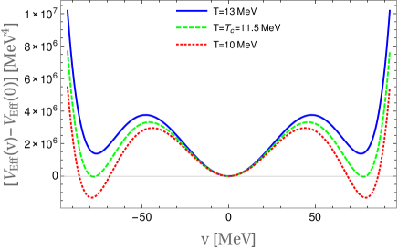
Figure 1: The effective potential, in the chiral limit, for a fixed value of chemical potential $\mu_{q}=322$ MeV and for values of temperature above, at and below the critical temperature $T_{c}$. Here, $T_{c}=11.5$ MeV.

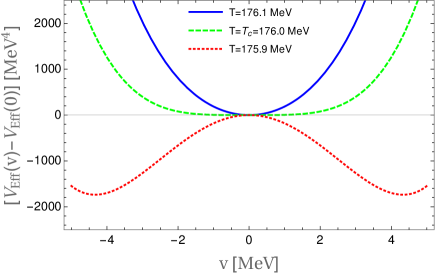
Figure 2: The effective potential, in the chiral limit, for $\mu_{q}=0$ MeV and for values of temperature above, at and below the critical temperature $T_{c}$. Here, $T_{c}=176.0$ MeV.

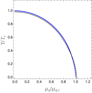
Figure 3: The phase diagram in the ($\mu_{q}$-$T$) plane. The solid and dashed curves are for the chiral limit ($h=0$) and correspond to the second-order and first-order transition lines, respectively. The dotted curve is for the physical case ($h\neq 0$) and represents a crossover transition. Temperature and chemical potential are normalized by the critical values in the chiral limit: $T_{c}=176$ MeV and $\mu_{q,c}=323$ MeV. For the crossover we have the pseudocritical values $T_{pc}=172$ MeV and $\mu_{q,pc}=329$ MeV.

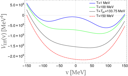
Figure 4: The effective potential in the physical case for a fixed value of chemical potential $\mu_{q}=220$ MeV. It shows a crossover phase transition as the temperature is changed. There is a pseudocritical temperature at $T_{pc}=133.75$ MeV determined by the position of the inflection point of the $\sigma$ field expectation value.

II.2.2 Physical case

When $h\neq 0$, the symmetry is never completely restored, with $v(T,\mu_{q})$ approaching zero for large values of $T$ and $\mu_{q}$. This behavior corresponds to a crossover transition. The gap equation gives

$$-m^{2}+\lambda v^{2}(T,\mu_{q}) =-\Pi_{\pi}^{\text{(ren)}}+\frac{h}{v(T,\mu_{q})}.$$ (32)

The pions are pseudo-Nambu-Goldstone bosons with mass squared $m_{\pi}^{2}=\frac{h}{v(T,\mu_{q})}$. The parameters are fixed by the same requirements as in the chiral limit and the extra condition on the pion masses in vacuum being set to their physical value $m_{\pi,0}=139\text{ MeV}$. For this case, we find the following set of parameters,

$$m^{2} =\lambda v_{0}^{2}-\frac{h}{v_{0}}\simeq(541.6\text{ MeV})^{2}\;, g \simeq 3.2\;,$$

$$\lambda =\frac{1}{2}\left(8\frac{N_{c}N_{f}}{(4\pi)^{2}}g^{4}+\frac{m_{\sigma}^{2}}{v_{0}^{2}}-\frac{h}{v_{0}}\right)\simeq 36.2\;, M^{2} =\frac{m_{q}^{2}}{e}\simeq(182.0\text{ MeV})^{2}\;,$$

$$h \simeq 1.8\cdot 10^{6}(\text{MeV})^{3}.$$ (33)

In the physical case, the effective potential exhibits a crossover transition, as shown in Fig. 4. Observe that the minimum of the potential moves smoothly towards zero as the temperature increases. The derivation of the crossover transition line on the ($\mu_{q}-T$) plane is performed numerically, with the result depicted in Fig. 3 together with the case for the chiral limit for comparison. In our computation, where we have considered both vacuum and thermal fluctuations for the fermions in the effective potential, we find only a crossover line. There are though other approximations where the crossover line can end and merge with a first-order phase transition line in a critical end point (see, e.g., Refs. Khan:2016exa ; Scavenius:2000qd ).

II.3 The pion string solution and its stability

In Ref. Zhang:1997is , Zhang et al. derived a stringlike classical solution in the LSM in the chiral limit and in the vacuum. Defining the new fields $\phi$ and $\pi^{\pm}$ as

$$\phi =\frac{\sigma+i\pi^{0}}{\sqrt{2}}, \pi^{\pm} =\frac{\pi^{1}\pm i\pi^{2}}{\sqrt{2}},$$ (34)

the $\Phi$-dependent part of the Lagrangian density is rewritten as

$$\mathcal{L}_{\Phi} =(\partial_{\mu}\phi)^{*}(\partial^{\mu}\phi)+(\partial_{\mu}\pi^{+})(\partial^{\mu}\pi^{-})-\lambda\left(\phi^{*}\phi+\pi^{+}\pi^{-}-\frac{v_{0}^{2}}{2}\right)^{2}.$$ (35)

Considering a static configuration, the energy functional, in the vacuum, reads

$$E_{0} =\int d^{3}x\left[\vec{\nabla}\phi^{*}\vec{\nabla}\phi+\vec{\nabla}\pi^{+}\vec{\nabla}\pi^{-}+\lambda\left(\phi^{*}\phi+\pi^{+}\pi^{-}-\frac{v_{0}^{2}}{2}\right)^{2}\right],$$ (36)

and the time-independent equations of motion are

$$\nabla^{2}\phi = 2\lambda\left(\phi^{*}\phi+\pi^{+}\pi^{-}-\frac{v_{0}^{2}}{2}\right)\phi\;,$$ (37)

$$\nabla^{2}\pi^{\pm} = 2\lambda\left(\phi^{*}\phi+\pi^{+}\pi^{-}-\frac{v_{0}^{2}}{2}\right)\pi^{\pm}.$$ (38)

These equations admit the following pion string solution:

$$\phi =\frac{v_{0}}{\sqrt{2}}\rho(r)e^{in\theta}\;, \pi^{\pm} =0,$$ (39)

where $r$ and $\theta$ are the polar coordinates in the $(x,y)$ plane and the integer $n$ is the winding number. The string has a linear extension in the $z$ direction.

The radial function $\rho(r)$ is found by substituting Eq. (39) into the equation of motion and using the boundary condition,

$$\rho(r)=\left\{\begin{array}[]{ll}0,&\;\;\;r\to 0,\\ 1,&\;\;\;r\to\infty,\end{array}\right.$$ (40)

leading to $\rho(r)\simeq(1-e^{-\mu r})$, where $\mu^{2}=2\lambda v_{0}^{2}$, and where $\mu^{-1}$ corresponds to the width of the string.

The above string solution is, however, nontopological. As it stands, once formed it will decay away. Since the vacuum manifold of this model is ${\cal M}=S^{3}$, there can be no topological defects vilenkin . In this case, the nontrivial field configuration can be continuously deformed to the vacuum. In other words, under an infinitesimal excitation of the fields $\pi^{\pm}$, the string configuration will unwind. To investigate the stability of the string, infinitesimal perturbations which involve the $\pi^{\pm}$ fields are considered. The perturbations induce a variation of the energy, and if this variation is negative, the string configuration will be unstable and decay. This is the case for the above pion string solution Zhang:1997is . However, if the effective potential in one of the field directions is lifted, in particular in the direction of the charged fields $\pi^{\pm}$, then we are left with an overall $U(1)$ symmetry of the effective potential in the $(\sigma,\pi^{0})$ directions. This then allows for a stable (embedded) topological pion string to form. This is the case studied by Nagasawa and Brandenberger in Nagasawa:1999iv , where they proposed a mechanism to stabilize the pion string by putting the system in a finite temperature plasma comprised of photons. The interaction between the charged pions and the electromagnetic field increases the effective potential in the $\pi^{\pm}$ directions. The potential for the $\pi^{\pm}$ fields acquires a quadratic term with a thermal mass contribution due to the coupling with the photons Karouby:2012yz , $e^{2}T^{2}\pi^{+}\pi^{-}/2$, which tends to stabilize the string.

III Pion string stability in a thermal and dense medium

III.1 Setup: Chiral limit

As shown in Ref. Nagasawa:1999iv , the interactions between the charged pions and the photons increase the effective potential in the $\pi^{\pm}$ directions and act to stabilize the string. We follow the same strategy but in addition to the thermal bath, we also consider the effect of the dense medium due to the interactions with the fermions. We assume that the fermions are in equilibrium with the thermal bath of photons, but, similar to Ref. Karouby:2012yz , the $\sigma$ and $\vec{\pi}$ fields are in a nonequilibrium state.

Using standard techniques bellac a nonzero chemical potential $\mu_{q}$ is set for the fermions and the thermal bath is implemented by the electromagnetic couplings between the charged particles of the model and the photon. In the minimal coupling prescription, the Lagrangian density becomes

$$\mathcal{L} =\mathcal{L}_{\Phi}+\mathcal{L}_{q}-\frac{1}{4}F_{\mu\nu}F^{\mu\nu}\;,$$ (41)

$$\mathcal{L}_{\Phi} =(\partial_{\mu}\phi)^{*}(\partial^{\mu}\phi)+(D^{+}_{\mu}\pi^{+})(D^{-\mu}\pi^{-})-\lambda\left(\phi^{*}\phi+\pi^{+}\pi^{-}-\frac{v_{0}^{2}}{2}\right)^{2}\;,$$ (42)

$$\mathcal{L}_{q} =\bar{\psi}\left\{i\gamma_{\mu}\left[\partial^{\mu}-ie\left(\begin{array}[]{cc}q_{u}&0\\ 0&q_{d}\end{array}\right)A^{\mu}\right]-\gamma^{0}\mu_{q}+g(\sigma+i\vec{\pi}\cdot\vec{\tau}\gamma_{5})\right\}\psi.$$ (45)

where $D^{\pm}_{\mu}=\partial_{\mu}\pm ieA_{\mu}$ and $q_{u}=2e/3$, $q_{d}=-e/3$ are the electric charges for the u quark and d quark, respectively.

The interactions with the thermal bath give a thermal mass to the charged particles, modifying the effective potential in the charged field directions Karouby:2012yz ,

$$\left.\Delta V_{\rm eff}\right|_{\text{Thermal Bath}} =\frac{e^{2}T^{2}}{4}\pi^{+}\pi^{-}.$$ (46)

Note also that the coupling to the photons gives a thermal mass bellac $m_{f}^{2}(T)=q_{f}^{2}T^{2}/8$ to the quarks as well. However, this term can be safely neglected with respect to the $gv$ term in the symmetry broken phase. In addition, at finite temperature and chemical potential, according to the gap equation (19), the expectation value of the $\sigma$ field is no longer equal to $v_{0}=f_{\pi}$, but depends on $T$ and $\mu_{q}$, $\langle\sigma\rangle=v\equiv v(T,\mu_{q})$.

In the following we will work in the chiral limit, $h=0$. To discuss the pion string in the thermal and dense medium, we use a mean-field approximation, in particular the Hartree method, by integrating out both the fermions and the electromagnetic gauge field $A_{\mu}$. The Hamiltonian field equations for $\sigma$ and $\pi_{i}$, $i=0,1,2$ are found to be

$$\nabla^{2}\sigma = \lambda\left(\sigma^{2}+\vec{\pi}^{2}-v_{0}^{2}\right)\sigma+g\langle{\bar{\psi}}\psi\rangle_{\rm(ren)},$$ (47)

$$\nabla^{2}\pi_{0} = \lambda\left(\sigma^{2}+\vec{\pi}^{2}-v_{0}^{2}\right)\pi_{0}+g\langle{\bar{\psi}}i\gamma_{5}\tau_{0}\psi\rangle_{\rm(ren)},$$ (48)

$$\nabla^{2}\pi_{1(2)} = \lambda\left(\sigma^{2}+\vec{\pi}^{2}-v_{0}^{2}\right)\pi_{1(2)}+g\langle{\bar{\psi}}i\gamma_{5}\tau_{1(2)}\psi\rangle_{\rm(ren)}+e^{2}\langle A_{\mu}A^{\mu}\rangle\pi_{1(2)},$$ (49)

where we have, in the Hartree-like approximation,

$$\langle A_{\mu}\rangle =0, \langle A_{\mu}A^{\mu}\rangle =\frac{T^{2}}{4},$$ (50)

and by taking the trace of the momentum integral of the fermion propagator, the scalar and pseudoscalar fermions densities are Scavenius:2000qd

$$\langle{\bar{\psi}}\psi\rangle = -2N_{c}N_{f}g\sigma\int\frac{d^{3}k}{(2\pi)^{3}}\frac{1}{\omega_{k}}\left[1-n_{F}^{+}(\omega_{k})-n_{F}^{-}(\omega_{k})\right]\;,$$ (51)

$$\langle{\bar{\psi}}i\gamma_{5}{\vec{\tau}}\psi\rangle = -2N_{c}N_{f}g{\vec{\pi}}\int\frac{d^{3}k}{(2\pi)^{3}}\frac{1}{\omega_{k}}\left[1-n_{F}^{+}(\omega_{k})-n_{F}^{-}(\omega_{k})\right].$$ (52)

Note that these depend explicitly on the $\sigma$ and $\vec{\pi}$ fields Csernai:1995zn . After subtracting the ultraviolet divergent term in the vacuum-dependent terms of the above momentum integrals, we have that the finite (renormalized) scalar and pseudoscalar fermion densities are, respectively,

$$\langle{\bar{\psi}}\psi\rangle_{\rm(ren)} = \sigma\,\Pi_{\pi}^{\rm(ren)}/g\;,$$ (53)

$$\langle{\bar{\psi}}i\gamma_{5}{\vec{\tau}}\psi\rangle_{\rm(ren)} = {\vec{\pi}}\,\Pi_{\pi}^{\rm(ren)}/g,$$ (54)

where $\Pi_{\pi}^{\rm(ren)}$ is given by Eq. (25).

Combining the above Eqs. (47)-(49) and expressing them in terms of $\phi=(\sigma+i\pi_{0})/\sqrt{2}$, $\pi^{\pm}=(\pi_{1}\pm i\pi_{2})/\sqrt{2}$ and also using Eq. (54) together with the massless pion condition in the chiral limit, Eq. (26), gives

$$\nabla^{2}\phi =2\lambda\left[\phi^{*}\phi+\pi^{+}\pi^{-}-\frac{v^{2}(T,\mu_{q})}{2}\right]\phi\;,$$

$$\nabla^{2}\pi^{\pm} =2\lambda\left[\phi^{*}\phi+\pi^{+}\pi^{-}-\frac{v^{2}(T,\mu_{q})}{2}+\frac{e^{2}T^{2}}{8\lambda}\right]\pi^{\pm}.$$ (55)

The above equations generalize the pion string equations in the vacuum, Eqs. (37) and (38). Hence, the pion string solution Eq. (39) for $\phi$ is modified to

$$\phi=\frac{v(T,\mu_{q})}{\sqrt{2}}{\tilde{\rho}}(r)e^{in\theta},$$ (56)

where $v(T,\mu_{q})$ is the solution of the gap equation (19), and ${\tilde{\rho}}$ has the same functional form as $\rho$ except that the inverse width is now given by $v(T,\mu_{q})$. The energy (36) is modified to

$$E_{0}\to E_{\rm eff} = \int d^{3}x\left\{\vec{\nabla}\phi^{*}\vec{\nabla}\phi+\vec{\nabla}\pi^{+}\vec{\nabla}\pi^{-}+\lambda\left[\phi^{*}\phi+\pi^{+}\pi^{-}-\frac{v(T,\mu_{q})^{2}}{2}\right]^{2}+\frac{e^{2}T^{2}}{4}\pi^{+}\pi^{-}\right\}.$$ (57)

III.2 Stability of the string core

To investigate the stability of the pion string core, we first consider a variation of the energy $\delta E$ of the string in the presence of infinitesimal perturbations of only the charged fields $\pi^{\pm}$,

$$\delta E =E_{\rm eff}-E_{\pi^{\pm}=0}=\int d^{3}x\left\{\vec{\nabla}\pi^{+}\vec{\nabla}\pi^{-}+\lambda\left[\frac{e^{2}T^{2}}{4\lambda}+2\phi^{*}\phi-v^{2}(T,\mu_{q})+\pi^{+}\pi^{-}\right]\pi^{+}\pi^{-}\right\}.$$ (58)

We use the ansatz (56) and expand the perturbations in the direction of $\pi^{\pm}$ as

$$\pi^{\pm} =v(T,\mu_{q})\sum_{m=0}^{\infty}\chi_{m}(r)e^{\pm im\theta}.$$ (59)

Using Eq. (59), the variation of the energy in cylindrical coordinates becomes

$$\delta E =2\pi v^{2}(T,\mu_{q})\int dz\int r\ dr\left\{\chi_{m}^{\prime 2}(r)+\frac{m^{2}}{r^{2}}\chi_{m}^{2}(r)+\left[\frac{e^{2}T^{2}}{4}+\lambda v^{2}(T,\mu_{q})({\tilde{\rho}}^{2}(r)-1)+\chi_{m}^{2}(r)\right]\chi_{m}^{2}(r)\right\}.$$ (60)

To determine the stability of the string, it is sufficient to know the overall sign of (60). A negative variation of energy would imply that the string configuration is not favored under an infinitesimal perturbation and would likely decay. Considering the integrand of the above equation, the first two terms $\chi_{m}^{\prime 2}$ and $\frac{m^{2}}{r^{2}}\chi_{m}^{2}$ are exact squares, so necessarily positive (in the next subsection we will explicitly analyze the effect of keeping these terms in the stability analysis). The only quantity that may give an instability is the last term. A sufficient condition of stability is therefore derived from the sign of

$$\left[\frac{e^{2}T^{2}}{4}+\lambda v^{2}(T,\mu_{q})({\tilde{\rho}}^{2}(r)-1)+\chi_{m}^{2}(r)\right].$$ (61)

The radial function $\chi_{m}$ is unknown; however, appearing as a square, it gives a positive contribution and so for obtaining a minimal condition for stability it can also be neglected. Using ${\tilde{\rho}}^{2}(r)-1\simeq e^{-{\tilde{\mu}}r}(e^{-{\tilde{\mu}}r}-2)$ [where ${\tilde{\mu}}$ is defined as $\mu$ except that $v_{0}$ is replaced by $v(T,\mu_{q})$], the variation of the mass per unit length compared to the embedded string is

$$\frac{e^{2}T^{2}}{4}-2\lambda v^{2}(T,\mu_{q})e^{-{\tilde{\mu}}r}(1-\frac{1}{2}e^{-{\tilde{\mu}}r})>0,$$ (62)

or, using that $e^{-{\tilde{\mu}}r}(1-\frac{1}{2}e^{-{\tilde{\mu}}r})\leq\frac{1}{2}$ for all $r$, we find

$$\frac{e^{2}T^{2}}{4}-\lambda v^{2}(T,\mu_{q})>0.$$ (63)

Figure 5: Stability region of the pion string core in a thermal and dense medium in the chiral limit. The parameters are those given by Eq. (31). The upper curve (blue) corresponds to the phase transition (second order). The dashed curve (red) corresponds to the lower limit of stability of the string. The range between the lines is the region of core stability.

We compute numerically the region of core stability using the parameters given in Eq. (31). Our results are shown in Fig. 5. The top line corresponds to the chiral phase transition, the string solution being nontrivial in the symmetry broken phase where $v(T,\mu_{q})$ is nonzero. The dashed line corresponds to the limit of stability $e^{2}T^{2}/4=\lambda v^{2}(T,\mu_{q})$. The model predicts a tiny ribbon for values of temperature and chemical potential, in between the two lines shown Fig. 5, for which stable string cores are allowed.

The size of the stability region is small, but the following argument makes plausible that such a region does indeed exist. We know from the results discussed for the LSMq in Sec. II.2 that the phase transition is of second order above the critical point. For a second order phase transition, the expectation value of the field is exactly zero on the transition line and then it moves away smoothly to finite values. There is always a region below the phase transition line where the expectation value $v(T,\mu_{q})$ is small enough to satisfy the stability condition $\eqref{eq:DMCond}$. We, therefore, expect that the stability condition is always satisfied for a second-order phase transition. This can be seen explicitly in the high-temperature approximation.

In the high-temperature region and close to the critical curve, such that $m_{q}/T\ll 1$, we use the approximation bellac

$$\int_{0}^{\infty}dk\frac{k^{2}}{\omega_{k}}\left[n_{F}^{+}(\omega_{k})+n_{F}^{-}(\omega_{k})\right]\simeq\int_{0}^{\infty}dkk\left[n_{F}^{+}(k)+n_{F}^{-}(k)\right]=\frac{\mu_{q}^{2}}{2}+\frac{\pi^{2}T^{2}}{6}\;,$$ (64)

and from the gap equation (20), we find (in the chiral limit $h=0$ and neglecting the vacuum contribution for simplicity)

$$\lambda v^{2}(T,\mu_{q})\approx\lambda v_{0}^{2}-\frac{N_{c}N_{f}}{\pi^{2}}g^{2}\left(\frac{\mu_{q}^{2}}{2}+\frac{\pi^{2}T^{2}}{6}\right)\;,$$ (65)

which using Eq. (63) leads to the approximate analytical stability condition,

$$\frac{e^{2}T^{2}}{4}-\lambda v_{0}^{2}+\frac{N_{c}N_{f}}{\pi^{2}}g^{2}\left(\frac{\mu_{q}^{2}}{2}+\frac{\pi^{2}T^{2}}{6}\right)>0\;.$$ (66)

Values for $T<T_{c}$ and $\mu_{q}<\mu_{c}$ can always be found, i.e., temperature and chemical potential below the values corresponding to those for the critical (second-order) transition line, such as to satisfy Eq. (66).

The situation changes drastically though when the transition is first order. It is well known that defects can form during a first-order phase transition as well (see, e.g. Hindmarsh:1993av ). In our model however, the strings would decay immediately. The stability condition relies on the smallness of the temperature and chemical potential background value $v(T,\mu_{q})$. Around the first-order transition the background value $v(T,\mu_{q})$ jumps (discontinuously) from zero in the symmetry restored phase to an usually higher value in the broken phase and the condition $\eqref{eq:DMCond}$ is never satisfied. Thus, we conclude that the existence of stable pion string cores depends strongly on the order of the phase transition. The stability condition for the pion string is favored around the second-order transition line of the phase diagram, but it is disfavored around the first-order transition region.

The stability condition Eq. (66) should be contrasted with the case where the Yukawa interactions are absent Nagasawa:1999iv , which leads to

$$\frac{e^{2}T^{2}}{4}-\lambda v_{0}^{2}>0.$$ (67)

Using the values given in Eq. (31) and that $e^{2}=4\pi/137$, we find that the temperature of the thermal bath required for the pion string core stability is

$$T_{\rm stab}>\frac{2f_{\pi}\sqrt{\lambda}}{e}\simeq 2.8\,{\rm TeV}.$$ (68)

This is, however, a temperature way above the critical temperature for chiral phase transition, $T_{c}\sim 176$ MeV. Thus, we conclude that it is simply not possible to have the stability condition satisfied since it only happens for temperatures for which the system is already in the symmetry restored phase. The inclusion of additional thermal and dense effects from the Yukawa interaction is thus fundamental for having a stable pion string core.

III.3 Stability in the physical case $h\neq 0$

In the physical case, $h\neq 0$, the effective potential leads to a crossover transition, as seen in Fig. 4. Defect formation in a crossover region is, unfortunately, very poorly understood at the moment, either from analytical studies or from numerical (lattice) simulations. As far as we know, there is just some limited discussion in the literature of defect formation for this case, such as for example Ref. Wenzel:2007uh , where it discusses how defects can be formed by percolation of different regions with different phases.

For the present case, when accounting only for the background fields, it would appear that no string solution can be constructed for the physical case of $h\neq 0$. As shown above, e.g. in Eq. (56), the pion string solution is constructed in the plane of the fields $(\sigma,\pi_{0})$, which is lifted with respect to the charged pions by the thermal electromagnetic plasma effect. The potential in the plane of the fields $(\sigma,\pi_{0})$, in the chiral limit $h=0$, is then of the form of a classical Mexican hat. The string solution interpolates between the unstable vacuum at the top of the potential to the infinitely degenerate minimum at the bottom of the potential. The solution then winds around the minima at the bottom of the potential with no cost of energy. This winding is possible due to the infinitely degenerate minimum of the potential (the pions are exactly Goldstone bosons). In the physical case, $h\neq 0$, the chiral symmetry is explicitly broken, the pions acquire mass and this winding freedom is no longer present (the potential now becomes a tilted Mexican hat). Under these circumstances, the string ansatz Eq. (56) no longer applies and for the background fields alone no string solution should be possible to construct.

The above situation, however, can change significantly when accounting for fluctuations of the fields in the thermal medium. Field fluctuations and gradient energies, which are negligible at zero temperature, can grow, particularly close to the transition and at large temperatures, where large fluctuations then start to become relevant. Under these conditions, it is then feasible that, as these fluctuations of the fields grow around the true vacuum of the system (the global minimum of the potential), they can be sufficiently large to probe the false vacuum state (the local minimum of the potential). When this happens, we can effectively say that the winding around the potential is once again restored, at least in localized regions of space. Much of the system will consist of regions of space where the fluctuations are small and the state is that of an explicitly chiral symmetry breaking as usual. However there will some regions with larger fluctuations where the chiral symmetry effectively looks restored, and such regions become increasingly more prevalent as the temperature increases. The pion strings that we are interested in are local objects, so all we need is some suitably large regions where conditions are appropriate for them to form. Thus, in regions of large fluctuations, where the chiral symmetry is effectively restored, pion string formation can become possible once again. This picture is similar to the mechanism discussed in Ref. Wenzel:2007uh for the formation of defects. Typical fluctuations in the fields have a spatial extent the size of the correlation length, with $\xi_{\sigma}^{-1}\sim m_{\sigma}$ and $\xi_{\pi}^{-1}\sim m_{\pi}$. As the temperature grows, these fluctuations start to become more and more frequent and eventually they start coalescing. In between these regions, string formation is possible, similar to the Kibble-Zurek mechanism of formation of defects in a second-order or even in a first-order phase transition Hindmarsh:1993av .

Though the physics of the formation of these fluctuations in a thermal medium and their consequences go beyond the analysis allowed within the framework of the effective potential, we can still provide some reasonable estimates for the importance of these fluctuation in the present problem.

Fluctuations in the fields around the true vacuum and that are large enough to probe the false vacuum of the potential should have an energy density in gradient form comparable to the difference in energy density between the false and true vacua of the potential,

$$\langle\frac{1}{2}{\vec{\nabla}}\sigma.{\vec{\nabla}}\sigma\rangle+\langle\frac{1}{2}{\vec{\nabla}}\pi.{\vec{\nabla}}\pi\rangle\approx hv,$$ (69)

where we have used that $\Delta V_{\rm eff}\simeq hv$ for the energy density difference. Assuming Gaussian-like (classical) correlation sized fluctuations for the fields in the thermal medium, we can then write Dziarmaga:1998js

$$\langle\frac{1}{2}{\vec{\nabla}}\sigma.{\vec{\nabla}}\sigma\rangle \simeq \frac{T}{4\pi^{2}}\int_{0}^{m_{\sigma}}dk\frac{k^{4}}{k^{2}+m_{\sigma}^{2}}$$ (70)

$$= (3\pi-8)\frac{m_{\sigma}^{3}T}{48\pi^{2}},$$

and analogous for the gradient energy density for the pion field.

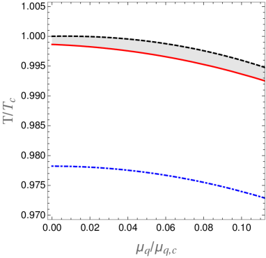
Figure 6: (a) The stability condition for the pion string (red line), the gradient energy condition (blue dot-dashed line) and the transition line (black dashed line), in the ($\mu_{q},T$) plane (normalized by the corresponding critical values). (b) An amplified view around the high-temperature, low chemical potential region. Strings are allowed to form in the shaded region below the transition line and above the stability condition.

In Fig. 6(a) we show the condition given by Eq. (69) alongside the transition line and the pion string stability line in the $(T,\mu_{q})$ plane in the physical case of $h\neq 0$. In Fig. 6(b) we zoom into a region similar to the one shown previously for the chiral limit in Fig. 5. We see from Fig. 6(a) that the gradient energy density is significantly closer to the transition line and remains slightly below it down to temperatures and chemical potential around $T\simeq 0.7T_{c}$ and $\mu_{q}\simeq 0.8\mu_{q,c}$, when it then goes above the transition line. In this region of large temperatures, the variations in the fields are sufficiently large to overcome the difference in potential energy density between the local and global minima of the potential. The stability condition, similar to what we have seen in the chiral limit $h=0$ (see, e.g., Fig. 5), is also very close to the transition line and slightly below it, lying in between the gradient energy condition and the transition line. In this small region of parameters, in between the stability condition (solid red line) and the transition line (dashed black line) and lying above the gradient energy condition (dash-dot blue line), is where pion strings can form (we locally recover the conditions for winding of the string) and be stable at the same time. Below the line for the gradient energy condition, the fluctuations of the fields (in terms of gradient energy) are not large enough to ensure the presence of strings, as discussed above.

The above analysis is just a preliminary examination of the physical case of $h\neq 0$ and it shows that pion string formation is plausible in this regime. More important, this section has laid out a conceptual framework for how to address this physical regime. An important general point that this analysis indicates is the importance that large fluctuations close to the transition may have on the formation, stability and presence of defects in general. A complete analysis would require a much more detailed treatment of the large localized fluctuations that emerge, such as through numerical simulations, which is beyond the scope of the present work. Nevertheless our analysis, though semiquantitative, indicates the importance that gradient energy densities for the fields can have on the pion string formation and subsequent stabilization when in a thermal and dense medium. These gradient energy terms can also have important effects in the subsequent evolution and decay of these strings when formed, as we discuss below. Our analysis here also shows that the role of fermions is an important ingredient to achieve stable pion strings even in the $h\neq 0$ case due to the effect they have on the order of the phase transition (recalling that in the absence of the fermion contributions, no stability is possible for physically motivated QCD parameters in this model). Thus the main focus of our paper on the role of fermions can be seen already to be important also for any detailed study of the $h\neq 0$ case.

III.4 Beyond string core stability

To study the overall stability of the pion string we need to consider the positive definite terms in $\delta E$ which were neglected in the previous subsections. They are in particular the radial gradient energy term of $\chi$ and the contribution of the $(\pi^{+}\pi^{-})^{2}$ term. The latter in fact blows up as we integrate out to large distances $r$ from the string core, unless $\chi$ goes to zero sufficiently fast for large values of $r$. In this case, the radial gradient energy of $\chi$ cannot be neglected. Also, if $\chi$ goes to zero at large values of $r$ it implies that the string winding in the neutral scalar field plane persists. Thus, even though the string core is unstable, the string will not totally decay.

To study this issue in more detail we will consider fluctuations which force the field to remain in the minimum potential energy density submanifold. Such a fluctuation is

$$|\phi|^{2}(r)\, = \,\rho^{2}(r)v^{2}{\rm cos}^{2}\xi(r)$$ (71)

$$\pi^{+}\pi^{-}(r) = \rho^{2}(r)v^{2}{\rm sin}^{2}\xi(r)\,,$$ (72)

where $v=v(T,\mu_{q})$ and the angle $\xi$ labels the magnitude of the perturbation. We focus on fluctuations which only depend on the radius since a nontrivial angular dependence would increase the energy density. For small $\xi$ and for $\xi$ independent of radius, this fluctuation reduces to the one considered in the previous subsection.

For this ansatz, the potential energy density vanishes exponentially for $r>v^{-1}$. However, associated with the nonvanishing value of $\pi^{+}\pi^{-}$ there is a contribution to the effective potential which comes from the temperature term. This can be minimized by having the profile of $\xi(r)$ decay beyond a width which we call $w$. In this case, the order of magnitude of the thermal effective potential energy gain $E_{th}$ is

$$E_{th}\,\sim\,\frac{e^{2}}{4}T^{2}w^{3}v^{2}\xi^{2}\,.$$ (73)

There is also a radial gradient energy $E_{grad}$ whose order of magnitude is

$$E_{grad}\,\sim\,v^{2}w\xi^{2}$$ (74)

since the gradient energy density scales as $vw^{-1}$ and the integration volume as $w^{3}$. The potential energy from the core region, on the other hand, decreases as $\xi^{2}$ increases. If $w>v^{-1}$ the potential energy $E_{pot}$ has an order of magnitude of

$$E_{pot}\,\sim\,\lambda v\bigl{(}1-2\xi^{2}\bigr{)}\,.$$ (75)

If $w<v^{-1}$ the change in potential energy is reduced by a factor of $(wv)^{3}$. The positive contributions to the total energy are thus minimized if we set $w\sim v^{-1}$. In this case, the stability condition of the core region becomes

$$\frac{\partial}{\partial\xi^{2}}\bigl{(}E_{th}+E_{grad}+E_{pot}\bigr{)}\,>\,1\,,$$ (76)

which yields

$$v^{2}(2\lambda-1)\,<\,\frac{e^{2}}{4}T^{2}\,.$$ (77)

If $\lambda\gg 1/2$ (which is the case for our pion string) then this condition reduces to the one (63) obtained in the previous subsection. However, for $\lambda<1/2$ we find that the string core is stable for all values of the temperature.

Let us now focus on the case $\lambda>{1/2}$. The above analysis shows that the string core will decay out to a radius of at least $w=v^{-1}$ if $T<T_{d}$, where $T_{d}$ is the temperature when (77) is saturated. But will the string decay completely? To answer this question we have to study what happens to the total energy change when $w$ increases beyond the value $v^{-1}$. We find that $\delta E$ is negative if

$$w\,<\,\left(\frac{4}{e^{2}}\right)^{1/3}T^{-2/3}v^{-1/3}\,\equiv\,w_{d}\,.$$ (78)

Hence, we conclude that the pion string winding remains for distances from the core larger than $w_{d}$. In this sense, the pion string in fact never completely decays, but simply undergoes “core melting.”

In a cosmological context, note that $w_{d}$ increases less fast as $T$ decreases compared to the Hubble radius which scales as $T^{-2}$. A pion string scaling solution with mean string separation given by the Hubble radius (the scaling solution which describes topologically stable cosmic strings) should hence be stable against total annihilation triggered by the core decay.

IV Conclusions

In this work we have investigated the effect of a thermal and dense medium on the stability of the pion string. We have used the LSMq model to describe the chiral phase transition using realistic physical parameters. We have constructed the corresponding pion string solution for the model, which depends explicitly now on the temperature and the chemical potential. Finally, using the mechanism similar to the one proposed in Ref. Nagasawa:1999iv , we have analyzed the stability for the pion strings and have derived a condition for it to be satisfied.

We have shown that at low temperatures, the pion string core will decay via the excitation of charged pion fields. However, the nontrivial winding of the neutral scalar fields persists at large distances from the core. In this sense, we should not speak of the pion string decay, but of pion string core melting. Whereas for the pion string configuration the energy density is confined to the core region, after core decay the energy will mainly be in field gradient energy which is dispersed out to a width $w_{d}$ [see (78)] which increases in time as the temperature decreases.

Our results have shown that the existence of a stable string core depends crucially on the order of the phase transition. Pion strings are produced and can become stable when the phase transition is second order. This happens because the expectation value of the field in the medium changes smoothly away from zero. In this case the stability condition is automatically satisfied in a region close to the transition line. This argument fails when the transition is first order since now the minimum of the potential can jump discontinuously to a large value, such that the stability condition no longer holds. In this respect the presence of fermions, which is a key direction this paper has explored, is crucial. The inclusion of the fermions indirectly provides stability, in the sense that fermions do not change the stability condition Eq. (63) but they change the order of the phase transition and therefore bring stability. This is a key new result of this paper and this is the first paper to find a stability region for the pion string. Although most of the analysis was done mainly in the chiral limit, in Sec. III.3 we have done a preliminary analysis also for the physical case of $h\neq 0$, where we have pointed out how fluctuations of the fields leading to large gradient energy densities, can play an important role in the formation and stability of pion strings in this regime.

The existence of pion strings has direct consequences for cosmology and nuclear physics. The region of the ($\mu_{q}-T$) plane in Fig. 3 with a second-order transition and stable strings has large temperatures and a low chemical potential. This region of the plane applies for both the early Universe and aspects of heavy-ion collision. The applications of the pion string in the early Universe are multiple. One concrete example is the creation of primordial magnetic fields as discussed in Ref. Brandenberger:1998ew . Pion strings in heavy-ion collisions experiments have been discussed recently in Refs. Mao:2004ym ; Lu:2015yua . The production of strings in these kinds of experiments may have an influence on the distribution of baryons and one could speculate about their experimental signature.

Another interesting area to investigate would be to find a further extension of the mechanism that stabilizes the string. In order to affect the effective potential in the constrained directions, one needs to act on the charged pions only. One possibility would be to place the system in an external magnetic field. We leave this as a possible future work.

Our work has applications beyond the LSMq of the strong interactions. Similar considerations can be used to study the stability of the Z string Vachaspati:1992fi , the embedded string solution made up of the uncharged complex Higgs field with the charged complex scalar set to zero. An initial study of the thermal stabilization of the Z string was given in Nagasawa2 . Our work shows that the Z string never completely decays, but at most undergoes core melting.

Looking beyond the Standard Model of strong, weak and electromagnetic interactions, and to higher temperatures, it would be interesting to study if there are embedded defects in beyond the Standard Model (BSM) theories which could be stabilized not only by a photon plasma, but by a plasma of the gauge fields which are massless above the electroweak symmetry breaking scale, and above the confinement scale. BSM theories with embedded domain wall solutions stabilized by a plasma in the early Universe could face severe cosmological problems since a single domain wall crossing our Hubble patch would overclose the Universe.