The IDSA and the Homogeneous Sphere:
Issues and possible improvements

Abstract.

In this paper, we are concerned with the study of the Isotropic Diffusion Source Approximation (IDSA) [6] of radiative transfer. After having recalled well-known limits of the radiative transfer equation, we present the IDSA and adapt it to the case of the homogeneous sphere. We then show that for this example the IDSA suffers from severe numerical difficulties. We argue that these difficulties originate in the min-max switch coupling mechanism used in the IDSA. To overcome this problem we reformulate the IDSA to avoid the problematic coupling. This allows us to access the modeling error of the IDSA for the homogeneous sphere test case. The IDSA is shown to overestimate the streaming component, hence we propose a new version of the IDSA which is numerically shown to be more accurate than the old one. Analytical results and numerical tests are provided to support the accuracy of the new proposed approximation.

Jérôme Michaud

Université de Genève, Section de Mathématiques,

2–4, rue du Lièvre, CP 64,

CH-1211 Genève

1. Introduction

In many astrophysical problems radiation plays a crucial role. As an example, core-collapse supernovæ   (CCSNe) explosion mechanisms crucially depend on the radiative transfer of neutrinos. In such practical calculation, the numerical computation of the full transfer equation is usually too costly and one has to rely on approximations.

In the context of CCSNe, Liebendörfer et al. [6] have designed the Isotropic Diffusion Source Approximation (IDSA). This approximation is based on asymptotic solutions of the radiative transfer equations, see [2] for a rigorous derivation of these asymptotic solutions; the coupling is then performed with the so-called Diffusion Source $\Sigma$ which has the form of a min-max switch. In [2], it is shown that this particular coupling mechanism might be problematic and mathematical issues are discussed. The aim of this paper is to study the behavior of the IDSA on a simple radiative transfer model and try to address some of the mathematical issues highlighted in [2].

The paper is organized as follows. In Section 2 we present the simple radiative transfer model to which we apply the IDSA. We also present the first three angular moments equation associated to it together with the well-known asymptotic limits of these equations, that is the diffusion limit, the reaction limit and the free streaming limit. Section 3 is devoted to the presentation of the IDSA adapted to our model problem. We discuss the three regimes of this approximation together with mathematical issues illustrated by numerical experiments. In Section 4, we discuss the homogeneous sphere test case and its limit of high opacities. We then reformulate the IDSA in order to remove the diffusion source $\Sigma$ and propose some modifications of the IDSA equations. In Section 5, we perform numerical experiments on the two new formulations of the IDSA and study their modeling error in the case of the homogeneous sphere. We conclude in Section 6 by discussing the different ways this work can be used in practical simulations of CCSNe explosions.

2. Radiative transfer equation and asymptotic limits

In this section, we consider the monochromatic (independent of energy) radiative transfer equation in spherical symmetry. We assume the background to be static and exclude inelastic and anisotropic scattering processes. The radiative transport equation in natural units ($c=1$) reads

$$\mathcal{L}_{\rm f}(f):=\partial_{t}f+\mu\partial_{r}f+\frac{1-\mu^{2}}{r}\partial_{\mu}f=\kappa_{\rm a}(b-f)+\kappa_{s}(J-f),$$ (1)

where $f(t,r,\mu)$ is the distribution function of the transported particles that depends on the time $t$, radius $r$ and cosine of the angle between the propagation direction and the radial direction $\mu$; $\kappa_{\rm a}(r)$ and $\kappa_{\rm s}(r)$ are the absorption and scattering opacities, respectively; $b(r,\mu)$ is the equilibrium distribution and $J(t,r)$ is the angular average of $f(t,r,\mu)$ defined in Eq. (4). We also introduce the linear transport operator $\mathcal{L}_{\rm f}$ of $f$. The first two moment equations are obtained by multiplying Eq. (1) by $1$ and $\mu$ respectively and integrating over $\mu$. This gives

$$\mathcal{L}_{\rm J}(J,H):=\partial_{t}J+\frac{1}{r^{2}}\partial_{r}(r^{2}H)=\kappa_{\rm a}(B-J),$$ (2)

and

$$\mathcal{L}_{\rm H}(J,H,K):=\partial_{t}H+\frac{1}{r^{2}}\partial_{r}(r^{2}K)+\frac{K-J}{r}=-(\kappa_{\rm a}+\kappa_{\rm s})H,$$ (3)

with the standard definitions

$$\{J,H,K\}:=\frac{1}{2}\int_{-1}^{1}d\mu\ \mu^{\{0,1,2\}}f.$$ (4)

The two moments equations (2) and (3) basically express the conservation of energy and momentum. The three angular moments $J,H$ and $K$ of the radiation field are proportional to the radiation energy density, flux and pressure. We also used the integrated equilibrium distribution $B=\frac{1}{2}\int_{-1}^{1}b\,d\mu$ and defined the transport operators $\mathcal{L}_{\rm J}$ and $\mathcal{L}_{\rm H}$ for $J$ and $H$, respectively. Note that these operators also depends on higher order moments and we obtain in general a hierarchy of equations that needs to be closed by a prescription of the form

$$H=H(J),\qquad K=K(H,J),$$ (5)

for a one-moment or a two-moment closure, respectively. A classical two-moment closure has been introduced in [5] and other two-moment closures are discussed in [9] in relation with flux-limited diffusion. It is also convenient to define the following flux factors.

Definition 2.1 (Flux ratio and variable Eddington factor).

The flux ratio $h(t,r)$ is defined by

$$h(t,r):=\frac{H(t,r)}{J(t,r)},$$ (6)

and the variable Eddington factor $k(t,r)$ is defined by

$$k(t,r):=\frac{K(t,r)}{J(t,r)}.$$ (7)

In order to enable a complete discussion of the IDSA, we need to discuss the asymptotic behavior of the radiative transfer equation because the IDSA is based on the coupling of three different asymptotic limits of this equation as shown in [2]. We discuss the diffusion limit, the reaction limit and the free streaming limit in terms of closure relations similar to Eq. (5).

2.1. Diffusion limit

Following [8, pp. 350–353], we can use the diffusion approximation of (1) by imposing the closure conditions

$$H=-\frac{1}{3\kappa}\frac{\partial J}{\partial r},\qquad K=\frac{1}{3}J,$$ (8)

where $\kappa:=\kappa_{\rm a}+\kappa_{\rm s}$ is the total opacity. These conditions lead to the diffusion equation

$$\mathcal{L}_{\rm J}^{\rm diff}(J):=\partial_{t}J-\frac{1}{r^{2}}\partial_{r}\left(r^{2}\frac{1}{3\kappa}\partial_{r}J\right)=\kappa_{\rm a}(B-J),$$ (9)

where we also defined the diffusive transport operator $\mathcal{L}_{\rm J}^{\rm diff}$ for $J$. In this limit, the variable Eddington factor satisfies

$$k^{\rm diff}(t,r)=\frac{1}{3}.$$ (10)

The diffusion limit is valid in regions where the mean free path $\kappa^{-1}$ is short compared with the typical length scale of the system. Such a region will be refered to as opaque. This limit can also be obtained by asymptotic expansions, see for example [2].

2.2. Reaction limit

The reaction regime is a special limit of the diffusion limit in which the total opacity $\kappa$ is so large that the diffusion term can be dropped in Eq. (9). This corresponds to the following closure relations

$$H=0,\qquad K=\frac{1}{3}J.$$ (11)

The corresponding evolution equation reads

$$\mathcal{L}_{\rm J}^{\rm reac}(J):=\partial_{t}J=\kappa_{\rm a}(B-J),$$ (12)

where we defined the reaction evolution operator $\mathcal{L}_{\rm J}^{\rm reac}$ for $J$ as before. The reaction limit is valid in regions where the mean free path $\kappa^{-1}$ is negligible compared with the typical length scale of the system. As for the diffusion limit, one can use asymptotic expansion with a different scaling in order to derive this limit, see for example [2].

2.3. Stationary state free streaming limit

The stationary state free streaming limit can be obtained by assuming that the free streaming particles have infinite velocity. As a result, the change of the distribution function is infinitely fast and one can drop the time derivative term in Eq. (2). We obtain

$$\mathcal{L}_{\rm J}^{\rm free}(J):=\frac{1}{r^{2}}\partial_{r}(r^{2}h^{\rm free}J)=\kappa_{\rm a}(B-J),$$ (13)

where the free streaming flux ratio can be estimated by a geometrical relation under the assumption that the streaming particles are emitted from an infinitely opaque homogeneous sphere of radius $R$. In this case, we have [3, 6]

Assumption 1 (Scattering sphere approximation).

The scattering sphere one-moment closure relation is given by the flux ratio

$$h^{\rm free}(r,R)=\left\{\begin{array}[]{ll}\displaystyle\frac{1}{2},&r<R,\\ \displaystyle\frac{1}{2}\left(1+\sqrt{1-\left(\frac{R}{r}\right)^{2}}\right),&r\geq R.\end{array}\right.$$ (14)

The radius $R$ is called the neutrinosphere radius.

This flux ratio corresponds, as we will rederive in Section 4, to the flux ratio of an infinitely opaque sphere of radius $R$. In Section 4 we also compute the corresponding variable Eddington factor. The neutrinosphere radius $R$ is usually computed using the optical depth $\tau$

$$\tau(r)=\int_{r}^{\infty}\kappa(r)dr$$ (15)

and the neutrinosphere radius satisfies $\tau(R)=\frac{2}{3}$.

As for the diffusion and the reaction limit, the stationary state free streaming limit can be derived by asymptotic expansions, see [2]. This approximation is valid where the mean free path $\kappa^{-1}$ is large compared with the typical length scale of the system. In these regions, the particles propagate freely and we therefore refer to them as transparent regions. In term of flux factor, the free streaming limit satisfies

$$\lim_{r\to\infty}h^{\rm free}(r,R)=1,\qquad\lim_{r\to\infty}k^{\rm free}(r,R)=1.$$ (16)

These limits come from the fact that in this case, the distribution function is strongly outward peaked and accumulates on $\mu=1$.

3. Isotropic Diffusion Source Approximation (IDSA)

As mentioned in Section 1, in practical calculations the direct solve of Eq. (1) is too costly and one need to rely on approximations. The Isotropic Diffusion Source Approximation (IDSA) has been developed by Liebendörfer et al. in [6] in the context of core-collapse supernovæ  (CCSNe) modeling. This is an approximation of the radiative transfer of neutrinos in this kind of stellar explosion. It is based on the observation that in a CCSN event, the inner core of the star becomes dense enough to be opaque to neutrinos, whereas the outer layers of the star are transparent. Following the discussion in Section 2, the radiative transfer of neutrinos in the inner core should be well described by the diffusion or the reaction limit, whereas in the outer layers it should be well described by the free streaming limit. This observation has led to the idea of using an additive decomposition of the distribution function into two components: a trapped component describing the inner core neutrinos and a free streaming component describing the outer layers neutrinos. Liebendörfer and colleagues also noted that it was enough, for their simulations, to compute the angular averaged $J$ distribution function. The IDSA is therefore an heterogeneous approximation of the first angular moment $J$ of the neutrino distribution function $f$. We now recall the hypotheses of the IDSA and state it for our model problem.

3.1. Ansatz: Decomposition into trapped and streaming neutrinos

We assume a decomposition of

$$f=f^{t}+f^{s}$$ (17)

on the whole domain into distribution functions $f^{t}$ and $f^{s}$ supposed to account for trapped and for streaming neutrinos, respectively. This ansatz is also valid for all the moments by linearity of integration

$$J = J^{t}+J^{s},$$ (18)

$$H = H^{t}+H^{s},$$ (19)

$$K = K^{t}+K^{s},$$ (20)

where we used the notation introduced in Eq. (4).

The IDSA is a two components one-moment approximation of Eq. (2) that we recall here

$$\mathcal{L}_{\rm J}(J,H)=\kappa_{\rm a}(B-J).$$ (21)

Assumption 2.

Eq. (21) can be well approximated by a system of equation of the form

$$\mathcal{L}^{t}_{\rm J}(J^{t},H^{t}(J^{t})) = \kappa_{\rm a}(B-J^{t})-\Sigma(J^{t},J^{s},B,\kappa_{\rm a},\kappa_{\rm s})$$ (22)

$$\mathcal{L}^{s}_{\rm J}(J^{s},H^{s}(J^{s})) = -\kappa_{\rm a}J^{s}+\Sigma(J^{t},J^{s},B,\kappa_{\rm a},\kappa_{\rm s})$$ (23)

$$\Sigma(J^{t},J^{s},B,\kappa_{\rm a},\kappa_{\rm s}) := \min\left\{\max\left[-\frac{1}{r^{2}}\partial_{r}\left(\frac{r^{2}}{3\kappa}\partial_{r}J^{t}\right)+\kappa_{\rm a}J^{s},0\right],\kappa_{\rm a}B\right\},$$ (24)

where $\Sigma$ is the diffusion source, and $J^{t}+J^{s}\approx J$.

The IDSA is completed by defining the operators $\mathcal{L}^{t}_{\rm J}$ and $\mathcal{L}^{s}_{\rm J}$ together with the closure relations for the trapped and the streaming components.

Assumption 3.

We assume that $f^{t}$, $\kappa_{\rm a}$ and $\kappa_{\rm s}$ are isotropic and that $f^{s}$ is in the stationary state free streaming limit. Hence, the IDSA uses the following closure relations

$$H^{t}(J^{t})=0,\qquad H^{s}(J^{s})=g_{\rm idsa}J^{s},$$ (25)

with $g_{\rm idsa}:=h^{\rm free}$. Comparing this closure relations with the asymptotic limits described in Section 2, we have the following operator definitions

$$\mathcal{L}^{t}_{\rm J}:=\mathcal{L}_{\rm J}^{\rm reac},\qquad\mathcal{L}^{s}_{\rm J}:=\mathcal{L}_{\rm J}^{\rm free}.$$ (26)

The IDSA is defined by Eqs (22)–(24) together with the closure relations given in Eq. (25) and the operator definitions given in Eq. (26).

Definition 3.1 (IDSA).

The IDSA equations are given by (dropping the dependence of $\Sigma$)

$$\mathcal{L}^{\rm reac}_{\rm J}(J^{t}) = \kappa_{\rm a}(B-J^{t})-\Sigma$$ (27)

$$\mathcal{L}^{\rm free}_{\rm J}(J^{s}) = -\kappa_{\rm a}J^{s}+\Sigma$$ (28)

$$\Sigma := \min\left\{\max\left[-\frac{1}{r^{2}}\partial_{r}\left(\frac{r^{2}}{3\kappa}\partial_{r}J^{t}\right)+\kappa_{\rm a}J^{s},0\right],\kappa_{\rm a}B\right\},$$ (29)

The diffusion source $\Sigma$ is defined in a way to switch between three different regimes to which we now come.

3.2. The three regimes of the IDSA

The IDSA has three distinct regimes corresponding to the different values that the diffusion source $\Sigma$ can take:

1. Reaction regime:

   $$\Sigma=0;$$

2. Diffusion regime:

   $$\Sigma=-\frac{1}{r^{2}}\partial_{r}\left(\frac{r^{2}}{3\kappa}\partial_{r}J^{t}\right)+\kappa_{\rm a}J^{s};$$

3. Free streaming regime:

   $$\Sigma=\kappa_{\rm a}B.$$

We now discuss these three regimes.

Remark 1.

In this work, when speaking about the behavior of the IDSA, we will speak about regimes. But when speaking about the asymptotic behavior of the real distribution, we will speak about limits. Hence, it is important to distinguish clearly between these two terms.

3.2.1. Reaction regime

In the reaction regime, the IDSA equations (27) and (28) become

$$\mathcal{L}^{\rm reac}_{\rm J}(J_{\rm reac}^{t}) = \kappa_{\rm a}(B-J_{\rm reac}^{t})$$ (30)

$$\mathcal{L}^{\rm free}_{\rm J}(J_{\rm reac}^{s}) = -\kappa_{\rm a}J_{\rm reac}^{s},$$ (31)

which shows that the trapped component is in the reaction limit, see Eq. (12) and $J_{\rm reac}^{s}$ is solution of Eq. (31), that is

$$J_{\rm reac}^{s}(r)=\frac{C}{r^{2}}{\rm e}^{-r\int_{0}^{r}h^{\rm free}(r)\,dr}.$$ (32)

Because $\frac{1}{2}\leq h^{\rm free}(r)\leq 1$, $J_{\rm reac}^{s}(r)>C\frac{{\rm e}^{-r^{2}}}{r^{2}}$ which diverges in $0$ in an unphysical way. Therefore, we have $C=0$ and

$$J^{\rm idsa}_{\rm reac}=J^{t}_{\rm reac}+J^{s}_{\rm reac}=J^{t}_{\rm reac},$$ (33)

and the solution of the IDSA in the reaction regime is in the reaction limit.

3.2.2. Diffusion regime

In the diffusion regime, the IDSA equations (27) and (28) become

$$\mathcal{L}^{\rm reac}_{\rm J}(J_{\rm diff}^{t}) = \kappa_{\rm a}(B-J_{\rm diff}^{t}-J_{\rm diff}^{s})+\frac{1}{r^{2}}\partial_{r}\left(\frac{r^{2}}{3\kappa}\partial_{r}J_{\rm diff}^{t}\right)$$ (34)

$$\mathcal{L}^{\rm free}_{\rm J}(J_{\rm diff}^{s}) = -\frac{1}{r^{2}}\partial_{r}\left(\frac{r^{2}}{3\kappa}\partial_{r}J_{\rm diff}^{t}\right),$$ (35)

or equivalently

$$\mathcal{L}^{\rm diff}_{\rm J}(J_{\rm diff}^{t}) = \kappa_{\rm a}(B-J_{\rm diff}^{t}-J_{\rm diff}^{s})$$ (36)

$$J_{\rm diff}^{s} = -\frac{1}{3\kappa h^{\rm free}}\partial_{r}J_{\rm diff}^{t},$$ (37)

that is the trapped component is in the diffusion limit up to a term of absorption of streaming particles. The first equation is obtained by passing the diffusion term on the left hand side, comparing with Eq. (9). The second is obtained by multiplying Eq. (35) by $r^{2}$ and integrating over $r$. This modified diffusion limit can also be obtained by asymptotic expansions, this has been shown in [2].

Remark 2.

Note that in order to have a positive distribution of streaming particles $J^{s}_{\rm diff}\geq 0$, it is necessary to have a decreasing distribution function of trapped $\partial_{r}J_{\rm diff}^{t}\leq 0$. That is, any non-decreasing solution of Eq. (36) is not physical.

Substituing (37) into (36), one can decouple the two equations and the new equation for the trapped particles is given by

$$\partial_{t}J_{\rm diff}^{t}-\frac{1}{r^{2}}\partial_{r}\left(r^{2}\frac{1}{3\kappa}\partial_{r}J_{\rm diff}^{t}\right)-\frac{\kappa_{\rm a}}{3\kappa h^{\rm free}}\partial_{r}J_{\rm diff}^{t}=\kappa_{\rm a}(B-J_{\rm diff}^{t}),$$ (38)

where we explicit the diffusion transport operator $\mathcal{L}^{\rm diff}_{\rm J}$.

3.2.3. Free streaming regime

In the free streaming regime, the IDSA equations (27) and (28) become

$$\mathcal{L}^{\rm reac}_{\rm J}(J_{\rm free}^{t})=\partial_{t}J_{\rm free}^{t} = -\kappa_{\rm a}J_{\rm free}^{t},$$ (39)

$$\mathcal{L}^{\rm free}_{\rm J}(J_{\rm free}^{s}) = \kappa_{\rm a}(B-J_{\rm free}^{s}),$$ (40)

which shows that the streaming component is in the stationary free streaming limit, see Eq. (13). The trapped equation can be solve analytically, we obtain

$$J_{\rm free}^{t}(t)=C{\rm e}^{-\kappa_{\rm a}t},$$ (41)

That is the trapped component is exponentially decreasing and vanishes in the stationary state.

3.3. Mathematical and numerical issues

We have discussed in Subsection 3.2 that the different regimes of the IDSA correspond to the asymptotic limit of the radiative transfer equation. The main problem of the IDSA is its treatment of transient regions where neither the diffusion, the free streaming nor the reaction limit apply. Then, nevertheless, one of the above regimes occurs. In the case of CCSN modeling, a discussion of this topic by numerical results comparing the IDSA with the full radiative transfer equation in the spherically symmetric case is given in [6]. In this paper, it is shown that the IDSA solution approximates pretty well the reference solution computed by solving the full radiative transfer equation. It is also shown that the biggest deviations occur in the “semi-transparent” transient region around the neutrinosphere. Similar results have been founded in a numerical example for a model problem in [1]. The limiters for the coupling term in (24) can be physically and mathematically motivated, see for example [6, 2], but there does not seem to be a rigorous explanation of these limitations by means of the full radiative transfer equation.

In the following, we take a closer look at some properties of the diffusion source $\Sigma$ and show that this coupling can lead to unphysical solutions and numerical instabilities.

3.3.1. Spurious trapped

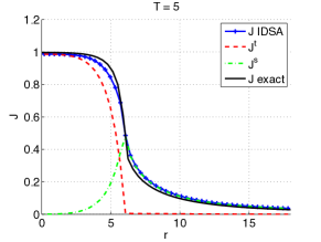
(a) Solution at time $T=5$.

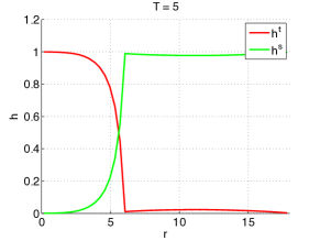
(b) Proportion of trapped $h^{t}=\frac{J^{t}}{J^{t}+J^{s}}$ and streaming particles $h^{s}=\frac{J^{s}}{J^{t}+J^{s}}$ at $T=5$.

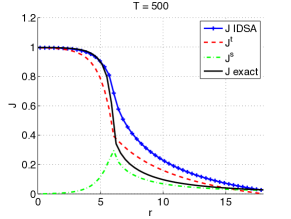
(c) Solution at time $T=500$.

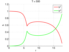
(d) Proportion of trapped $h^{t}=\frac{J^{t}}{J^{t}+J^{s}}$ and streaming particles $h^{s}=\frac{J^{s}}{J^{t}+J^{s}}$ at $T=500$.

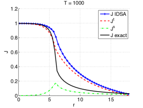
(e) Solution at time $T=1000$.

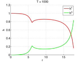
(f) Proportion of trapped $h^{t}=\frac{J^{t}}{J^{t}+J^{s}}$ and streaming particles $h^{s}=\frac{J^{s}}{J^{t}+J^{s}}$ at $T=1000$.

Figure 1. Results for the IDSA with small opacity $\kappa_{\rm a}=10^{-3}$ for $r\geq 6$. The different panels show the evolution of the distributions. The black curve displays the solution of the homogeneous sphere. The right panels illustrate the takeover of trapped particles in the streaming region.

The first problem that we discuss here is referred to as the Spurious Trapped problem. This is a problem in modeling that occurs in regions with small but non zero opacities ($\kappa$ small). The problem originates in the definition of the coupling term $\Sigma$. Such a region should be transparent and therefore described by the free streaming limit. Hence, the IDSA limiter should always choose the free streaming regime in this case. We now construct an example in which the definition of diffusion source $\Sigma$ leads to a wrong regime.

Proposition 1.

In a transparent region where $\kappa_{\rm a}=\mathcal{O}(\varepsilon)$ and where the distribution $J^{t}$ is locally constant and $J^{s}<B$, we have

$$\Sigma\neq\kappa_{\rm a}B,$$ (42)

that is the IDSA does not choose the free streaming regime in this case.

Proof.

The condition on $\kappa_{\rm a}$ is needed in order to have a transparent region, for more details about this asymptotic limit, see [2, 7]. We now compute the value of the diffusion source in this case.

$$\Sigma =\min\left\{\max\left[-\frac{1}{r^{2}}\partial_{r}\left(\frac{r^{2}}{3\kappa}\partial_{r}J^{t}\right)+\kappa_{\rm a}J^{s},0\right],\kappa_{\rm a}B\right\}$$ (43)

$$=\min\left\{\max\left[\kappa_{\rm a}J^{s},0\right],\kappa_{\rm a}B\right\},$$

where we used the fact that $J^{t}$ is locally constant. We now observe that $\kappa_{\rm a}>0$ and that $J^{s}<B$ by hypothesis, this leads to

$$\Sigma=\kappa_{\rm a}J^{s}<\kappa_{\rm a}B.$$ (44)

This concludes the proof. ∎

We now discuss the relevance of the hypotheses used in Proposition 1. As we have mentioned in the proof, the assumption on $\kappa_{\rm a}$ just reflects the fact that we are in a transparent region. In such a region, Eq. (41) implies that the trapped distribution vanishes. Finally, the condition on $J^{s}$ is natural in radiative transfer problems. In fact, the equilibrium distribution is mainly driven by emission and absorption processes which are small in a transparent region. The transport processes therefore tend to reduce the distribution which leads to $J^{s}<B$.

Now that we know that the hypotheses can be realized, we look at the resulting dynamics of the trapped particles

$$\partial_{t}J^{t}=\kappa_{\rm a}(B-J^{t}-J^{s}).$$ (45)

Because $B-J^{s}>0$, we can assume that there exists $B^{\prime}$ such that $B-J^{s}\geq B^{\prime}>0$ and

$$J^{t}>B^{\prime}(1-{\rm e}^{-\kappa_{\rm a}t})$$ (46)

that is, the trapped particle distribution is growing.

Remark 3.

Note that if $\kappa_{\rm a}=0$ in the free streaming regime, a non-vanishing trapped distribution will not be eliminated because its evolution becomes

$$\partial_{t}J^{t}_{\rm free}=0.$$ (47)

and the distribution, whatever it is at first, is stationary.

Now that we have seen that the spurious trapped problem may occur, we show a numerical illustration of this problem. For the discretization, we used the discretization proposed by Liebendörfer in [6] described in more detail in [1, 7]. For the grid parameters, we choose $N_{r}=50$ and $\Delta t=0.1$. For the parameters of the radiative transfer equation, we choose $B=1$, $\kappa_{\rm s}=0$ and

$$\kappa_{\rm a}=\left\{\begin{array}[]{ll}1,&\text{if }r<R=6,\\ \varepsilon=10^{-3},&\text{if }r\geq R=6.\end{array}\right.$$ (48)

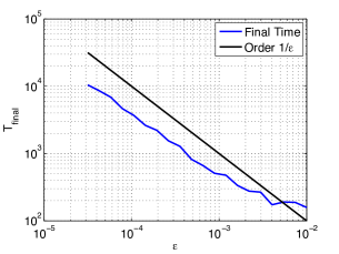
Figure 2. Time needed to reach a stationary distribution dominated by spurious trapped particles with respect to $\varepsilon$.

The results are displayed in Figure 1. In this Figure, we also show the proportions $h^{t}=\frac{J^{t}}{J^{t}+J^{s}}$ and $h^{s}=\frac{J^{s}}{J^{t}+J^{s}}$ of trapped and streaming particles on the right panels. This illustrates the fact that the trapped component is growing. This problem develops on a slow timescale, and becomes visible only on a long timescale. When $\varepsilon$ goes to zero, the time needed to create spurious trapped particles tends to infinity and this problem disappears. In Figure 2, we display the time needed to reach a stationary distribution dominated by spurious trapped particles in the streaming region. The results show that the time needed to reach a stationary state grows roughly with an order of $\mathcal{O}(\varepsilon^{-1})$. Numerically, a linear regression on the results presented in Figure 2, where we excluded the $5$ first points because for too big $\varepsilon$ the free streaming limit is no longer a good approximation, gives an order of $\mathcal{O}(\varepsilon^{-0.90})$. It is reasonable to think that inside a CCSN, the time interval over which the solution is computed is too short for this problem to develop.

3.3.2. Instability of the coupling

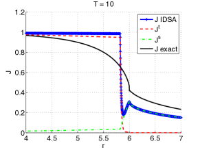
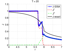
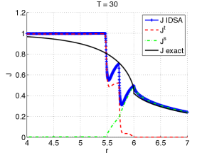
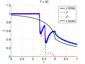
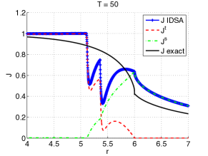
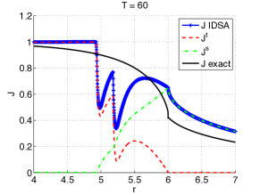
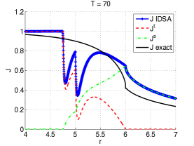
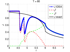
Figure 3. Development of the instability. These results have been obtained with an homogeneous sphere example defined by $\kappa=\mathds{1}_{r<6}$. The figure illustrates the formation of the instability and its inward propagation.

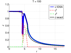
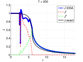
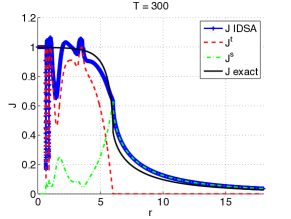
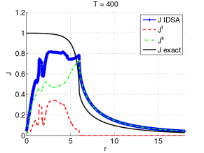
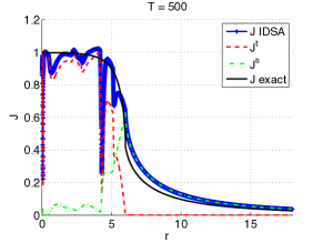
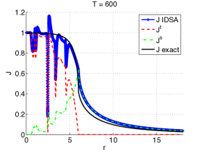
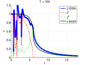
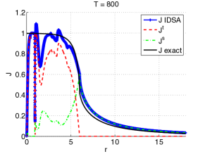
Figure 4. Long time behavior of the instability. These results have been obtained with a homogeneous sphere example defined by $\kappa=\mathds{1}_{r<6}$. The figure illustrates the long time behavior of the solution.

The second problem we discuss is also linked with the diffusion source $\Sigma$. It takes the form of an instability that develops at a boundary between an opaque and a transparent region. It originates in the fact that the diffusion term in $\Sigma$ can become large for two reasons: the first is because $\kappa$ is small and the domain is transparent, and this triggers a correct transition to the streaming limit; the second is because the concavity becomes large. At the boundary between a very opaque and a transparent region, the second case may occur leading to a switch to the streaming regime in a region where the opacity $\kappa$ is large. That is, where the diffusion limit is valid and the diffusion regime of the IDSA should apply. As a consequence, the IDSA virtual boundary between the opaque and the transparent domains is shifted inward. This shift is helped by the creation of streaming particles that feed back into the dynamics of the trapped particles in the form of an inward advection term, see Eq. (38). At some point, the diffusion limit is recovered near the real boundary and starts to grow again as expected, but at the virtual boundary of the IDSA, the trapped distribution continues to locally decrease leading to a locally radially growing distribution of trapped particles which is not physical, see Remark 2. As an effect, an instability of the underlying model is created and propagated inward.

As a numerical illustration of such an instability, we apply the IDSA to the homogeneous sphere test case defined by $\kappa_{\rm s}(r)=0$, $\kappa_{\rm a}(r)=\mathds{1}_{r<6}$ and $B=1$. For the grid parameters, we set $N_{r}=10^{4}$ and $\Delta t=0.1$.

Figure 3 displays the formation of the instability near the boundary of the homogeneous sphere. We see for example in the first subfigure that the virtual boundary of the IDSA, where the trapped distribution vanishes, stands at a radius $r<R$. This illustrates the shift of the interface discussed above. The next subfigures show the early developement of the instability and its inward transport due to the feedback of the streaming component into the trapped component dynamics, see Eq. (38).

The behavior of the solution on longer times is displayed in Figure 4. This figure shows the evolution of the instability. The solution becomes more complicated as time passes. Note that the solution remains bounded and never explodes like a usual numerical instability due to numerical problems such as a CFL condition. This instability in the solution comes from the modeling and the definition of the coupling term $\Sigma$.

Remark 4.

The instability is linked with the size of the diffusion term. Note that this quantity also depends on the discretization as the second derivative will be of the order of $\mathcal{O}((\Delta r)^{-2})$. This means that if the discretization is coarse enough, then the instability does not occur. This explains the fact that we used a coarse grid in the spurious trapped numerical experiment. In fact, if we refine the grid, the spurious trapped numerical experiment will also show the numerical instability that we just described.

We have shown with these two examples that the coupling in the IDSA equations can lead to wrong solutions that are due to the application of a wrong asymptotic regime in parts of the domain. This can lead to the creation of spurious trapped particles or to the creation of an instability in the solution. We have also discussed the influence of the advection term coming from the coupling with streaming particles in the trapped diffusion equation. It seems that this term helps the developement of the instability.

A natural question to ask is: why did the IDSA work in the case of the CCSN models performed in [6]? We answer this question below.

3.4. Why does the IDSA work in practice?

As we mentioned in Section 1, in the numerical tests performed by Liebendörfer et al. in [6], the IDSA is quite accurate and good enough to be used in simulations. We just discussed two important mathematical issues of this approximation. How is it possible that the IDSA works in practice when it fails on simple examples? Part of the answer has been given in Remark 4. If the discretization is coarse enough, the instability can not develop. In the application of the IDSA to the CCSN modeling, the number of grid points is $N_{r}=1000$ and the repartition of points is such that the instability of the underlying model does not develop. However, it is probable that a refinement of the radial grid will lead to the apparition of an instability in the IDSA. Note that in a real CCSN simulation, the reactions in the center become very large and as a result, the instability is quickly damped. In our example for the instability, we used an artificially small opacity $\kappa=1$. For larger opacities, the instability is damped and vanishes in the limit of the infinitely opaque homogeneous sphere. Another possible explanation is that in the CCSN numerical experiments, the radiative transfer equation is coupled to the background matter. This coupling is done through the trapped particles and their distribution is reconstructed at every time step with a smoothing effect that may help to get rid of the instability. Regarding the spurious trapped particles, we have observed that the growing of the spurious trapped particles component is slow and that it takes a long time to dominate the dynamics, if ever. In fact, in a CCSN simulation, the time window on which the neutrino radiative transfer needs to be computed is short and the spurious trapped particles do not contribute significantly to the dynamics.

We now study in full detail the case of the homogeneous sphere where an analytical solution is known. This idealized example will shed light on the coupling mechanism and will help us to partly correct or avoid the problems we have described.

4. The case of the stationary homogeneous sphere

In this example we want to solve the monochromatic equation (1) with $\kappa_{\rm s}=0$, that is

$$\partial_{t}f+\mu\partial_{r}f+\frac{1-\mu^{2}}{r}\partial_{\mu}f=\kappa_{\rm a}(B-f).$$ (49)

We assume that the equilibrium distribution $B$ is constant. The homogeneous sphere setting is completed by requiring a specific form for $\kappa_{\rm a}$. We set

$$\kappa_{\rm a}=\kappa\mathds{1}_{r<R}\,,$$ (50)

where $\kappa$ is a constant and $\mathds{1}$ is the characteristic function. This example has been chosen for two main reasons. The first is because it has a closed form solution that is for example derived in Chapter 2 of Duderstadt and Martin [4]. The second reason is that this example naturally has two different regions where the limit dynamics correspond to the limits used in the derivation of the IDSA. It is therefore a very good and natural case study for the IDSA.

The steady state radiative transfer equation (49) has an analytical solution given by

$$f(r,\mu)=B(1-{\rm e}^{-\kappa s(r,\mu)}),$$ (51)

where

$$s(r,\mu)=\left\{\begin{array}[]{llr}\displaystyle r\mu+RG(r,\mu)&r<R,&-1<\mu<1,\\ 2RG(r,\mu)&r\geq R,&\displaystyle\left[1-\left(\frac{R}{r}\right)^{2}\right]^{1/2}<\mu<1,\end{array}\right.$$ (52)

and

$$G(r,\mu):=\left[1-\left(\frac{r}{R}\right)^{2}(1-\mu^{2})\right]^{1/2}.$$ (53)

This solution is easily obtained from the formal solution of the transport equation; see e.g. [4].

The first three angular moments of the analytical exact solution are given by

$$J(r)=\left\{\begin{array}[]{lr}\displaystyle B\left[1-\int_{0}^{1}d\mu\cosh(\kappa r\mu){\rm e}^{-\kappa RG(r,\mu)}\right]&r<R,\\ \\ \displaystyle\frac{B}{2}\left[1-\sqrt{1-\left(\frac{R}{r}\right)^{2}}-\int_{\sqrt{1-(\frac{R}{r})^{2}}}^{1}d\mu{\rm e}^{-2\kappa RG(r,\mu)}\right]&r\geq R,\end{array}\right.$$ (54)

and

$$H(r)=\left\{\begin{array}[]{lr}\displaystyle B\int_{0}^{1}d\mu\mu\sinh(\kappa r\mu){\rm e}^{-\kappa RG(r,\mu)}&r<R,\\ \\ \displaystyle\frac{B}{2}\left[\frac{1}{2}\left(\frac{R}{r}\right)^{2}-\int_{\sqrt{1-(\frac{R}{r})^{2}}}^{1}d\mu\,\mu{\rm e}^{-2\kappa RG(r,\mu)}\right]&r\geq R,\end{array}\right.$$ (55)

and

$$K(r)=\left\{\begin{array}[]{lr}\displaystyle B\left[\frac{1}{3}-\int_{0}^{1}d\mu\mu^{2}\cosh(\kappa r\mu){\rm e}^{-\kappa RG(r,\mu)}\right]&r<R,\\ \\ \displaystyle\frac{B}{6}\left[1-\left(1-\left(\frac{R}{r}\right)^{2}\right)^{3/2}\!\!\!\!\!-3\int_{\sqrt{1-(\frac{R}{r})^{2}}}^{1}d\mu\mu^{2}{\rm e}^{-2\kappa RG(r,\mu)}\right]\!\!&r\geq R,\end{array}\right.$$ (56)

and can be computed by direct integration from Equation (51) using the parity of the function $G(r,\mu)$ with respect to $\mu$.

We now give some particular values of the analytical solutions that will be useful for the analysis of the IDSA.

Proposition 2.

The values of $J$ and $H$ at $r=0$ and at $r=R$ are

$$J(0) = B(1-{\rm e}^{-\kappa R}),$$ (57)

$$J(R) = \frac{B}{2}\left[1+\frac{{\rm e}^{-2\kappa R}-1}{2\kappa R}\right],$$ (58)

$$H(0) = 0,$$ (59)

$$H(R) = \frac{B}{2}\left[\frac{1}{2}+{\rm e}^{-2\kappa R}\left(\frac{1}{2\kappa R}+\frac{1}{(2\kappa R)^{2}}\right)-\frac{1}{(2\kappa R)^{2}}\right].$$ (60)

Proof.

The proof is done by direct integration. ∎

Before applying the IDSA to the homogeneous sphere, we discuss the limit of the homogeneous sphere when the opacity $\kappa\to\infty$. We call this limit the infinitely opaque homogeneous sphere.

For the stationary distribution function (51), we have the following limit

$$\lim_{\kappa\to\infty}f(r,\mu)=\left\{\begin{array}[]{ll}0,&\displaystyle\text{if }r\geq R,\ -1<\mu\leq\left[1-\left(\frac{R}{r}\right)^{2}\right]^{1/2},\\ B,&\text{otherwise.}\end{array}\right.$$ (61)

For the first three angular moments, we have

$$\lim_{\kappa\to\infty}J(r)=\left\{\begin{array}[]{lr}\displaystyle B&r<R,\\ \displaystyle\frac{B}{2}\left[1-\sqrt{1-\left(\frac{R}{r}\right)^{2}}\right]&r\geq R,\end{array}\right.$$ (62)

and

$$\lim_{\kappa\to\infty}H(r)=\left\{\begin{array}[]{lr}0&r<R,\\ \displaystyle\frac{B}{2}\left[\frac{1}{2}\left(\frac{R}{r}\right)^{2}\right]&r\geq R,\end{array}\right.$$ (63)

and

$$\lim_{\kappa\to\infty}K(r)=\left\{\begin{array}[]{lr}\displaystyle\frac{B}{3}&r<R,\\ \displaystyle\frac{B}{6}\left[1-\left(1-\left(\frac{R}{r}\right)^{2}\right)^{3/2}\right]&r\geq R.\end{array}\right.$$ (64)

These results directly come from Eqs (54)–(56) by noting that the dependence on $\kappa$ is contained only in the integral terms that vanish when $\kappa\to\infty$ as shown in the following proposition.

Proposition 3.

Integrals of the form

$$I_{1} = \int_{0}^{1}d\mu\mu^{\{0,2\}}\cosh(\kappa r\mu){\rm e}^{-\kappa RG(r,\mu)},$$ (65)

$$I_{2} = \int_{0}^{1}d\mu\mu\sinh(\kappa r\mu){\rm e}^{-\kappa RG(r,\mu)},$$ (66)

$$I_{3} = \int_{\sqrt{1-(\frac{R}{r})^{2}}}^{1}d\mu\,\mu^{\{0,1,2\}}{\rm e}^{-2\kappa RG(r,\mu)},$$ (67)

vanish when $\kappa\to\infty$.

Proof.

The proof for $I_{3}$ is clear as the only dependence on $\kappa$ is in the exponential. The proof for $I_{1}$ and $I_{2}$ relies on the fact that the integrants satisfy

$$\mu^{\{0,2\}}\cosh(\kappa r\mu){\rm e}^{-\kappa RG(r,\mu)} = \mathcal{O}({\rm e}^{\kappa(r\mu-RG(r,\mu))}),$$ (68)

$$\mu\sinh(\kappa r\mu){\rm e}^{-\kappa RG(r,\mu)} = \mathcal{O}({\rm e}^{\kappa(r\mu-RG(r,\mu))}),$$ (69)

because the behavior of $\cosh$ and $\sinh$ is dominated by their positive exponential parts. For $I_{1}$ and $I_{2}$ to vanish in the limit $\kappa\to\infty$, it is sufficient to check that $r\mu-RG(r,\mu)<0$ for $r<R$, or equivalently, because all these quantities are positive, that $(r\mu)^{2}-(RG(r,\mu))^{2}<0$ for $r<R$. We obtain

$$(r\mu)^{2}-(RG(r,\mu))^{2} =(r\mu)^{2}-R^{2}+r^{2}(1-\mu^{2})$$ (70)

$$=-R^{2}+r^{2}<0,\quad\text{since }r<R.$$

This concludes the proof. ∎

In this limit, we can compute the variable Eddington factor $k=\frac{K}{J}$ and the flux factor $h=\frac{H}{J}$ defined in Definition 2.1.

Proposition 4.

In the limit $\kappa\to\infty$ the flux factor $h_{R}$ and the variable Eddington factor $k_{R}$ of the homogeneous sphere of radius $R$ are given by

$$h_{R}(r)=\frac{H(r)}{J(r)}=\left\{\begin{array}[]{ll}0,&r<R,\\ \displaystyle\frac{1}{2}\left(1+\sqrt{1-\left(\frac{R}{r}\right)^{2}}\right),&r\geq R,\end{array}\right.$$ (71)

and

$$k_{R}(r)=\frac{K(r)}{J(r)}=\left\{\begin{array}[]{ll}\displaystyle\frac{1}{3},&r<R,\\ \displaystyle\frac{1}{3}\left(2-\left(\frac{R}{r}\right)^{2}+\sqrt{1-\left(\frac{R}{r}\right)^{2}}\right),&r\geq R.\end{array}\right.$$ (72)

Proof.

The proof is done by direct computation from equations (62)-(64). ∎

With these results on the behavior of the analytical solution of the homogeneous sphere, we can now study the IDSA in this particular case.

4.1. Applying the IDSA to the homogeneous sphere

In order to apply the IDSA to the homogeneous sphere test case and to overcome the numerical problems illustrated in Subsection 3.3, we need to reformulate the IDSA. This is done by introducing the following assumption.

Assumption 4.

We assume that the radius $R$ of the homogeneous sphere corresponds to the neutrinosphere radius. We also assume that

1. The domain of validity of the diffusion and the reaction regimes is characterized by $r<R$.

2. The domain of validity of the free streaming regime is characterized by $r\geq R$.

This is a very important assumption because it allows us to avoid the problematic diffusion source $\Sigma$ and to realize the coupling directly and explicitly. This way, we eliminate both the spurious trapped and the instability problem discussed above and we will have access to the modeling error of the IDSA.

Remark 5.

Assumption 4 allows us to simplify the Eqs (31) and (32) for the streaming particles and (35) and (37) for the trapped particles, recalling (13), because the function $h^{\rm free}=g_{\rm idsa}=\frac{1}{2}$ in these cases.

Remark 6.

We remark here that Assumption 4 does not match the usual definition of the neutrinosphere based on the optical depth, see Eq. (15). In fact, in the case of the homogeneous sphere, one can compute the neutrinosphere radius $R_{\nu}$

$$\int_{R_{\nu}}^{\infty}\kappa_{\rm a}(r)dr=\kappa\int_{R_{\nu}}^{R}dr=\kappa(R-R_{\nu})=\frac{2}{3},$$ (73)

where we used the definition of $\kappa_{\rm a}$, see Eq. (50); that is, the usual definition of the neutrinosphere radius only corresponds to the homogeneous sphere radius in the limit $\kappa\to\infty$ as $R-R_{\nu}=\frac{2}{3\kappa}$.

Remark 7 (IDSA in the limit $\kappa\to\infty$).

In the limit $\kappa\to\infty$, the diffusion limit is irrelevant and we have the following solution

$$J^{t}_{\rm reac}(r,t) = B,\quad r<R,$$ (74)

$$J^{s}_{\rm reac}(r,t) = 0,\quad r<R,$$ (75)

$$J^{t}_{\rm free}(r,t) = 0,\quad r\geq R,$$ (76)

$$J^{s}_{\rm free}(r,t) = C(t)\frac{2}{R^{2}}\left(1-\sqrt{1-\left(\frac{R}{r}\right)^{2}}\right),\quad r\geq R.$$ (77)

If we set $C(t):=\frac{R^{2}B}{4}$, the solution of this coupling is equivalent to the analytical solution (62) of the infinitely opaque homogeneous sphere. This condition can be ensured by requiring the boundary condition $J^{s}_{\rm free}(R,t)=\frac{B}{2}$.

Using Assumption 4 and Remark 5, one can rewrite the IDSA equations (37)–(40) without reaction and with $\kappa=0$ for $r\geq R$ as

$$\begin{array}[]{rclr}\displaystyle\partial_{t}J^{t}-\frac{1}{r^{2}}\partial_{r}\left(\frac{r^{2}}{3\kappa}\partial_{r}J^{t}\right)-\frac{2}{3}\partial_{r}J^{t}&=&\kappa(B-J^{t}),&r<R,\\ J^{s}&=&\displaystyle-\frac{2}{3\kappa}\partial_{r}J^{t},&r<R,\\ J^{t}&=&0,&r\geq R,\\ \displaystyle\frac{1}{r^{2}}\partial_{r}\left(r^{2}g(r)J^{s}\right)&=&0,&r\geq R,\end{array}$$ (78)

with $g(r)=\frac{1}{2}\left(1+\sqrt{1-\left(\frac{R}{r}\right)^{2}}\right)$ the geometrical factor appearing in Eq. (14).

It is possible to reconstruct the first and second angular moments $H$ and $K$ by defining flux factors for the trapped and the free streaming components. We set

$$h^{t}_{R}:=0,\qquad h^{s}_{R}:=\left\{\begin{array}[]{ll}\displaystyle\frac{1}{2},&r<R,\\ \displaystyle\frac{1}{2}\left(1+\sqrt{1-\left(\frac{R}{r}\right)^{2}}\right),&r\geq R,\end{array}\right.$$ (79)

and

$$k^{t}_{R}:=\frac{1}{3},\qquad k^{s}_{R}:=\left\{\begin{array}[]{ll}\displaystyle\frac{1}{3},&r<R,\\ \displaystyle\frac{1}{3}\left(2-\left(\frac{R}{r}\right)^{2}+\sqrt{1-\left(\frac{R}{r}\right)^{2}}\right),&r\geq R.\end{array}\right.$$ (80)

Remark 8.

We note that the definition of $h^{s}_{R}$ corresponds to the definition of $h^{\rm free}=g_{\rm idsa}$, see Eq. (14). In fact, this definition can be used as a justification for the definition of $g_{\rm idsa}$ in the derivation of the IDSA. The definition of these flux factors extend the stationary free streaming limit to the first order moment solution.

Proposition 5.

With Equations (79) and (80), we can reconstruct $H_{\rm idsa}(r)$ and $K_{\rm idsa}(r)$ through the relations

$$H_{\rm idsa}(r) = h^{t}_{R}(r)J^{t}(r)+h^{s}_{R}(r)J^{s}(r)=h^{s}_{R}(r)J^{s}(r),$$ (81)

$$K_{\rm idsa}(r) = k^{t}_{R}(r)J^{t}(r)+k^{s}_{R}(r)J^{s}(r).$$ (82)

This reconstruction has the following properties:

1. IDSA closure in the diffusion regime:

   $$H_{\rm idsa}=-\frac{1}{3\kappa}\partial_{r}J^{t},\ \text{if }r<R.$$

2. Free streaming flux ratio:

   $$h^{s}_{R}(r)=h^{\rm idsa}_{R}(r)=h_{R}(r),\ \text{if }r\geq R.$$

3. Diffusion variable Eddington factor:

   $$k^{\rm idsa}_{R}(r)=\frac{1}{3}=k_{R}(r),\ \text{if }r<R.$$

4. Free streaming variable Eddington factor:

   $$k^{s}_{R}(r)=k^{\rm idsa}_{R}(r)=k_{R}(r),\ \text{if }r\geq R,$$

where $h_{R}$ and $k_{R}$ are the flux factors for the infinitely opaque homogeneous sphere and $h^{\rm idsa}_{R}:=\frac{H_{\rm idsa}}{J^{t}+J^{s}}$ and $k^{\rm idsa}_{R}:=\frac{K_{\rm idsa}}{J^{t}+J^{s}}$ are the IDSA flux factors.

Proof.

We prove separatly the four points.

1. The first statement can be proved by inserting Eqs (79) and (78) into Eq. (81).

2. In the region $r\geq R$, we have $J^{t}=0$. As a consequence, $h_{R}^{s}=h^{\rm idsa}_{R}=h_{R}$ by Eqs (79) and (71).

3. In the region $r<R$, we have $k^{t}_{R}=k^{s}_{R}=1/3$. Therefore,

   $$K_{\rm idsa}(r)=k^{t}_{R}(r)J^{t}(r)+k^{s}_{R}(r)J^{s}(r)=\frac{1}{3}(J^{t}(r)+J^{s}(r))=\frac{1}{3}J_{\rm idsa}(r).$$

   The proof is completed by comparing this result with Eq. (72).

4. The proof of this point is similar to the proof of 2.

This concludes the proof. ∎

The proposition 5 shows that the flux factors of the IDSA correspond to the flux factors of the infinitely opaque homogeneous sphere. However, the flux ratio of the IDSA in the diffusion region $r<R$ does not match the diffusion limit relation (8) even if the form is similar. In fact,

$$H_{\rm idsa}=-\frac{1}{3\kappa}\partial_{r}J^{t}\neq-\frac{1}{3\kappa}\partial_{r}J_{\rm idsa}=-\frac{1}{3\kappa}\partial_{r}J^{t}+\frac{2}{9\kappa^{2}}\partial^{2}_{r}J^{t},$$ (83)

where we used Eq. (78)₂ to eliminate the streaming component in the last equality. This means that the diffusion limit is not well represented by this formulation. Moreover, the diffusion equation (38) used for the trapped particles does not correspond to the usual diffusion approximation equation (9).

Another possible problem of this formulation is that the amount of streaming particles at the homogeneous sphere radius is not necessarily accurate. If this value is inaccurate, then the error will be propagated by the free streaming equation in the whole domain where $r\geq R$. This can create large approximation errors.

In order to deal with the problem of the advection term and the possible inaccuracy of the amount of streaming particles at the homogeneous sphere radius, we propose in the next subsection some possible modifications of the approximation.

4.2. Improvements of the scheme

We now propose some improvements of the IDSA. We propose to use the diffusion equation (9) instead of Eq. (78)₁ for the evolution of the trapped particles and to modify the reconstruction of the streaming particles in the diffusion regime to correctly predict the amount of streaming particles at the homogeneous sphere radius. This is done through the following assumption

Assumption 5.

In the diffusion region, we assume that the free streaming component can be reconstructed from the trapped component by a relation of the form

$$J^{s}(r)=C\partial_{r}J^{t}.$$ (84)

The constant $C$ is chosen in such a way that $J^{s}(R)=J(R)=\frac{B}{2}\left[1+\frac{{\rm e}^{-2\kappa R}-1}{2\kappa R}\right]$, see Proposition 2.

The scheme obtained can be written as

$$\begin{array}[]{rclr}\displaystyle\partial_{t}J^{t}-\frac{1}{r^{2}}\partial_{r}\left(\frac{r^{2}}{3\kappa}\partial_{r}J^{t}\right)\!\!\!\!&=&\!\!\!\!\kappa(B-J^{t}),&r<R,\\ J^{s}\!\!\!\!&=&\!\!\!\!\displaystyle C\partial_{r}J^{t}=\frac{B}{2}\left[1+\frac{{\rm e}^{-2\kappa R}\!-1}{2\kappa R}\right]\frac{\partial_{r}J^{t}}{\partial_{r}J^{t}|_{r=R}},\!\!\!&r<R,\\ J^{t}\!\!\!\!&=&\!\!\!\!0,&r\geq R,\\ \displaystyle\frac{1}{r^{2}}\partial_{r}\left(r^{2}g(r)J^{s}\right)\!\!\!\!&=&\!\!\!\!0,&r\geq R,\end{array}$$ (85)

where $g(r)=\frac{1}{2}\left(1+\sqrt{1-\left(\frac{R}{r}\right)^{2}}\right)$. The results 2.–4. of Proposition 5 still hold and the point 1. can be rephrased as

• $H_{\rm idsa}=\frac{C}{2}\partial_{r}J^{t}$, if $r<R$.

The proof of this fact closely follows the proof of point 1. of Proposition 5.

The scheme ensures that the trapped particles are evolved by a diffusion equation and that the amount of streaming particles is correct in the whole domain where $r\geq R$. Another advantage of this formulation is that it has a stationary state closed form solution.

In the stationary state limit, we can compute the closed form solution of system (85) given in the following proposition.

Proposition 6.

The closed form solution of the stationary state limit of (85) is given by

$$\begin{array}[]{rclr}J^{t}(r)&=&\displaystyle B\left(1-\frac{R}{r}\frac{\sinh(\sqrt{3}\kappa r)}{\sinh(\sqrt{3}\kappa R)}\right),&r<R,\\ J^{s}(r)&=&\displaystyle C\frac{3\kappa^{2}BR}{\sinh(\sqrt{3}\kappa R)}\left(\frac{\sinh(\sqrt{3}\kappa r)}{(\sqrt{3}\kappa r)^{2}}-\frac{\cosh(\sqrt{3}\kappa r)}{\sqrt{3}\kappa r}\right),&r<R,\\ J^{t}(r)&=&0,&r\geq R,\\ J^{s}(r)&=&\displaystyle\frac{B}{2}\left[1+\frac{{\rm e}^{-2\kappa R}-1}{2\kappa R}\right]\left(1-\sqrt{1-\left(\frac{R}{r}\right)^{2}}\right),&r\geq R,\end{array}$$ (86)

where $C=\frac{R}{2}\left[1+\frac{{\rm e}^{-2\kappa R}-1}{2\kappa R}\right]\left(1-\frac{\sqrt{3}\kappa R}{\tanh(\sqrt{3}\kappa R)}\right)^{-1}$.

Proof.

To prove this proposition, it is enough to substitute the proposed solution into system (85) and checking that it is a solution. ∎

Remark 9.

The trapped component of the solution (86) has the property to have a negative radial derivative that vanishes at $r=0$, see for example [7, Chap. 4]. This ensures that the streaming component is positive. The vanishing at $r=0$ property motivates the use of a Neumann boundary condition at this point.

Proposition 6 gives a closed form solution of the new version of the IDSA. It can be shown that the total solution $J_{\rm idsa}=J^{t}+J^{s}$ is bounded by $B$. As a consequence of Remark 9, we have $J^{s}(0)=0$ and $J_{\rm idsa}(0)=J^{t}(0)=B\left(1-\frac{\sqrt{3}\kappa R}{\sinh(\sqrt{3}\kappa R)}\right)$, since $\lim_{x\to 0}\frac{\sinh(x)}{x}=1$. This value has to be compared with the value of the solution of the homogeneous sphere given in Proposition 2.

This comparison leads to the following result.

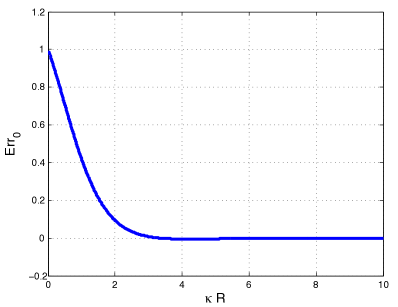
Figure 5. Plot of the value of ${\rm Err}_{0}$ as a function of $\kappa R$. The plot shows that if $\kappa R$ is large enough, the error in $r=0$ vanishes.

Proposition 7.

The relative error at $r=0$ of the New IDSA approximation (86) is given by

$${\rm Err}_{0}=\frac{\left(\frac{\sqrt{3}\kappa R}{\sinh(\sqrt{3}\kappa R)}-{\rm e}^{-\kappa R}\right)}{(1-{\rm e}^{-\kappa R})}.$$ (87)

Proof.

It suffices to substract the evaluation of (86)₁ at $r=0$, using the fact that $\lim_{x\to 0}\frac{\sinh(x)}{x}=1$, from (57) and divide by Eq. (57). ∎

The value of ${\rm Err}_{0}$ can be used as a measure of the validity of the New IDSA approximation (85).

Figure 5 shows that the error vanishes when $\kappa R$ is large. This figure also shows that the approximation fails when $\kappa R$ is small, that is when the diffusion approximation is not valid, as expected.

5. Numerical experiments

For the numerical experiments, we apply the two versions of the IDSA designed before to the homogeneous sphere test case. We refer to Eq. (78) as the Old IDSA approximation and to Eq. (85) as the New IDSA approximation. We use a backward Euler scheme with a finite difference scheme in space with a very fine grid, $N_{r}=10^{6}$. Such a fine grid eliminates discretization errors and the remaining discrepancy can be attributed to modeling error. We use $0$ initial conditions and boundary conditions are discussed in [7, Chap.4].

The test case we choose is an homogeneous sphere of radius $R=6$. The value of $\kappa$ is varied in the different tests.

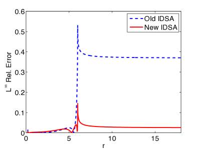
Figure 6. Plot of the pointwise relative error of the Old IDSA (in blue) and of the New IDSA (in red) applied to the homogeneous sphere of radius $R=6$ and $\kappa=1$.

As a first example, we apply the Old IDSA and the New IDSA to the homogeneous sphere of radius $R=6$ with $\kappa=1$. Figure 6 shows the relative approximation error of these two schemes. We notice that the Old IDSA (in blue) has a considerably larger error in the free streaming region where $r\geq R$ than the New IDSA (in red). These results show that even if the flux factors are accurate and the diffusion relation given in Proposition 5 is satisfied by the Old IDSA approximation, it does not mean that the approximation is good. The modifications given is Section 4.2 greatly improve the situation. The error still has a peak at the homogeneous sphere radius, but this is expected as a consequence of the definition of approximations (78) and (85). A better view of this example is given in Figure 7 where we also give the value of the flux factors $h$ and $k$ which can be computed from the value of $J^{t}$ and $J^{s}$ from Proposition 5.

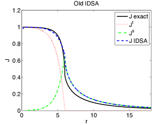
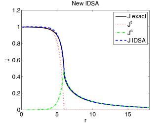
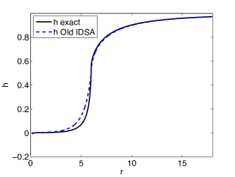
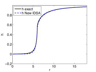
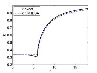
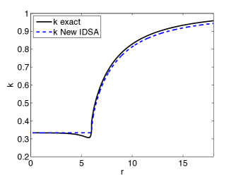
Figure 7. Results of the Old IDSA (on the left) and of the New IDSA (right) on the homogeneous sphere of radius $R=6$ with $\kappa=1$. The first line gives the value of $J$, the second gives the flux ratio $h$ and the third gives the variable Eddington factor $k$. The exact solution is given by the black line and numerical results are given in blue. For the results of $J$, the trapped component is given in red and the free streaming component in green.

The results show that the Old IDSA overestimates the value of streaming particles at the radius of the homogeneous sphere; this leads to an overestimation of the streaming particles in the whole region where $r\geq R$, explaining the results of Figure 6. We also notice that, compared to the New IDSA, the Old IDSA underestimates the proportion of the trapped particles and overestimates the proportion of the streaming particles in the diffusive region ($r<R$). In a CCSN experiment, the overestimation of streaming particles can lead to larger heating rates behind the shock and an artificially increased likeliness for explosions. From this viewpoint, one would say that the Old IDSA overestimates the neutrino heating, see [6]. Regarding the flux factors, we see in Figure 7 that the flux ratio of the Old IDSA is worse that the flux ratio of the New IDSA; that is the correction done in the $J$ distribution reflects in the flux ratio. There are, however, no differences in the approximation of the variable Eddington factors. This is a consequence of the reconstruction of $H_{\rm idsa}$ and $K_{\rm idsa}$ given in Proposition 5 from which the flux factors are computed.

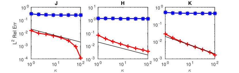
Figure 8. Plot of the convergence of the $L^{2}$ relative errors for the homogeneous sphere test case. The radius of the homogeneous sphere is $R=6$ and $\kappa$ is varied from $1$ to $100$. The results of the Old IDSA (in blue) do not converge when $\kappa\to\infty$ whereas the results of the New IDSA (in red) converge to the exact solution of the homogeneous sphere. The numerical rate of convergence is of the order $\mathcal{O}(\kappa^{-1/2})$ for all the quantities.

To complement the study, we let the values of $\kappa$ vary from $1$ to $100$ and compute the relative $L^{2}$ errors. In Figure 8, we see that the errors of the Old IDSA (in blue) do not converge even if the flux factors are pretty accurate according to Figure 7, whereas the errors of the New IDSA (in red) converge to the exact values of $J$, $H$ and $K$ of the homogeneous sphere given in (54)–(56). The numerical order of convergence of these three quantities is $\mathcal{O}(\kappa^{-1/2})$. This rate of convergence has only been obtained numerically and we want to prove this fact in future work.

The first panel of Figure 8 shows that the convergence of $J$ accelerates for large values of $\kappa$, but this behavior has yet to be understood.

6. Conclusion and outlook

In this paper, we have discussed the behavior of the IDSA on the homogeneous sphere test case. We have shown that the current implementation of this approximation has modeling issues coming from the definition of the coupling mechanism, that is from the diffusion source $\Sigma$. The two main problems are the Spurious Trapped and Instability problems. In the case of the homogeneous sphere, we have changed the coupling mechanism assuming the different regions where each regime apply to be known. Doing so, the two modeling problems are avoided allowing us to access the modeling error of the IDSA. We show with numerical experiments that the IDSA is overestimating the streaming component both in the diffusive and in the free streaming part of the domain. To address the other issue, we proposed a new version of the IDSA based on the analytical solution of the homogeneous sphere. This very particular model has been shown to converge to the solution of the infinitely opaque homogeneous sphere case. We also used the analytical solution of this case to obtain the flux ratio and the variable Eddington factor for the stationary state free streaming limit used in the IDSA. The new version of the IDSA presented has also been shown to converge for the first and second order moments with these flux factors. The order of convergence has been numerically estimated to $\mathcal{O}(\kappa^{-1/2})$ and the proof of this fact is still missing.

We have shown in this paper that simplifying the model can shed some light on the behavior of the approximation. To go further in the analysis, we need to go back to more complicated radiative transfer problems. The analysis presented in this work is very specific to the homogeneous sphere example. However, many astrophysical problems do have a very similar structure, a dense body surrounded by a transparent atmosphere. This is the case for example in CCSN simulations, stellar winds, planetary disks and many other astrophysical problems. A possible direction in which our results can be extended is to use the neutrinosphere radius as the limiting radius for trapped particles. Note that Remark 6 shows that these two radius are usually not equal, but close when $\kappa$ is large. This allows the computation of trapped particles with the New IDSA scheme. Then, one needs to find a way to reconstruct the streaming particle distribution inside the neutrinosphere in order to obtain a boundary condition for the transport of streaming neutrinos outside the neutrinosphere. Once such a condition is obtained, one can use any radiative transfer code to compute the outside distribution.

Received xxxx 20xx; revised xxxx 20xx.

References

- [1] H. Berninger, E. Frénod, M. Gander, M. Liebendörfer, J. Michaud and N. Vasset, A Mathematical Description of the IDSA for Supernova Neutrino Transport, its Discretization and a Comparison with a Finite Volume Scheme for Boltzmann’s Equation, in ESAIM: Proc., CEMRACS’11: Multiscale Coupling of Complex Models in Scientific Computing, vol. 38, 2012, 163–182.
- [2] H. Berninger, E. Frénod, M. Gander, M. Liebendörfer, J. Michaud and N. Vasset, Derivation of the IDSA for Supernova Neutrino Transport by Asymptotic Expansions, SIMA, 45 (2013), 3229–3265.
- [3] S. Bruenn, Stellar core collapse: Numerical model and infall epoch, Astrophys. J. Suppl. S., 58 (1985), 771–841.
- [4] J. J. Duderstadt and W. R. Martin, Transport Theory, John Wiley & Sons, 1979.
- [5] C. Levermore and G. Pomraning, A flux-limited diffusion theory, The Astrophysical Journal, 248 (1981), 321–334.
- [6] M. Liebendörfer, S. Whitehouse and T. Fischer, The Isotropic Diffusion Source Approximation for Supernova Neutrino Transport, Astrophys. J., 698 (2009), 1174–1190.
- [7] J. Michaud, From Neutrino Radiative Transfer in Core-Collapse Supernovae to Fuzzy Domain Based Coupling Methods, PhD thesis, Université de Genève, 2015.
- [8] D. Mihalas and B. Weibel-Mihalas, Foundation of Radiation Hydrodynamics, Oxford University Press, 1984.
- [9] J. Smit, L. Van den Horn and S. Bludman, Closure in flux-limited neutrino diffusion and two-moment transport, Astronomy and Astrophysics, 356 (2000), 559–569.