From superdeformation to extreme deformation and clusterization in the $N\sim Z$ nuclei of the $A\sim 40$ mass region.

Abstract

A systematic search for extremely deformed structures in the $N\sim Z$ nuclei of the $A\sim 40$ mass region has been performed for the first time in the framework of covariant density functional theory. At spin zero such structures are located at high excitation energies which prevents their experimental observation. The rotation acts as a tool to bring these exotic shapes to the yrast line or its vicinity so that their observation could become possible with future generation of $\gamma-$tracking (or similar) detectors such as GRETA and AGATA. The major physical observables of such structures (such as transition quadrupole moments as well as kinematic and dynamic moments of inertia), the underlying single-particle structure and the spins at which they become yrast or near yrast are defined. The search for the fingerprints of clusterization and molecular structures is performed and the configurations with such features are discussed. The best candidates for observation of extremely deformed structures are identified. For several nuclei in this study (such as ³⁶Ar), the addition of several spin units above currently measured maximum spin of $16\hbar$ will inevitably trigger the transition to hyper- and megadeformed nuclear shapes.

I Introduction

There is a considerable interest to the study of cluster structures and extremely deformed shapes in light nuclei Kanada-En’yo and Kimura (2005); von Oertzen et al. (2006); Maruhn et al. (2006); Taniguchi et al. (2007); Reinhard et al. (2011); Ebran et al. (2012); Taniguchi (2014); Zhao et al. (2015); Iwata et al. (2015); Jenkins (2016). Many of these structures are described in terms of clusters, the simplest one being the $\alpha$-particle von Oertzen et al. (2006); Maruhn et al. (2006). Providing a unique insight on the cluster dynamics inside of nucleus, the initial assumptions about clusters represent a limitation of this type of models. Note also that many shell model configurations are beyond the reach of the cluster models. It is also important to remember that the cluster description does not correspond to clearly separated $\alpha$-particles, but generates the mean-field states largely by antisymmetrization Maruhn et al. (2006). In addition, the studies of molecular structures, which appear in many extremely deformed configurations, have gained considerable interest Kimura and Horiuchi (2004); von Oertzen et al. (2006); Taniguchi (2014).

In recent years, the investigations of exotic cluster configurations have been undertaken also in the density functional theory (DFT). The advantage of the DFT framework is the fact that it does not assume the existence of cluster structures; the formation of cluster structures proceeds from microscopic single-nucleon degrees of freedom via many-body correlations Ebran et al. (2012, 2014). As a result, the DFT framework allows simultaneous treatment of cluster and mean-field-type states Egido and Robledo (2004); Reinhard et al. (2011); Ebran et al. (2012, 2014); Yao et al. (2014). It is important to mention that covariant (relativistic) energy density functionals (CEDFs) show more pronounced clusterization of the density distribution as compared with non-relativistic ones because of deeper single-nucleon potentials Ebran et al. (2012).

Let us mention some recent studies of cluster and extremely deformed structures in the DFT framework. The clustering phenomenon in light stable and exotic nuclei was studied within the relativistic mean field (RMF) approach in Ref. Arumugam et al. (2005) and within the Hartree-Fock (HF) approach based on the Skyrme energy density functionals (EDF) in Ref. Reinhard et al. (2011). Linear chain configurations of four $\alpha$-clusters in ¹⁶O and the relationship between the stability of such states and angular momentum were investigated using Skyrme cranked HF method in Ref.  Ichikawa et al. (2011) and cranked RMF (further CRMF) in Ref. Yao et al. (2014). This is an example of the “rod shaped” nucleus. Another case of such structures is linear chain of three $\alpha$ clusters, suggested about 60 years ago Morinaga (1956); it was recently studied in the CRMF theory in Ref. Zhao et al. (2015). This exotic structure (“Hoyle” state) plays a crucial role in the synthesis of ¹²C from three ⁴He nuclei in stars Hoyle (1954). The stability of rod-shaped structures in highly-excited states of ²⁴Mg was studied in Ref. Iwata et al. (2015) in cranked Skyrme HF calculations.

The difficulty in investigating cluster and extremely deformed states is that they are generally unbound and lie at high excitation energies at low spins von Oertzen et al. (2006); Jenkins (2016). Moreover, they are either formed on the shoulder or in very shallow minima of potential energy surfaces Ebran et al. (2014); Afanasjev and Abusara (2008); thus, they are inherently unstable at low spin. The high density of nucleonic configurations at these energies and possible mixing among them is another factor hindering their observation with current and future generations of experimental facilities. Moreover, obtaining unambiguous evidences for clustering (such as a transition strengths between different states and the structure of the wavefunction) is equally challenging and frequently ambiguous from experimental point of view. In addition, the mechanisms of the reactions used in experimental studies frequently favor the population of yrast or near-yrast states Jenkins (2016).

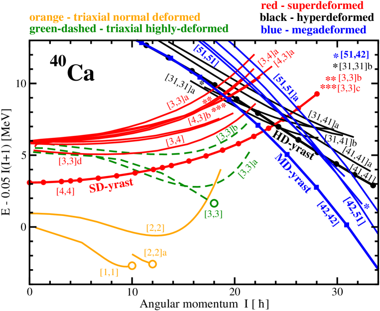
Figure 1: (Color online) Energies of the calculated configurations in ⁴⁰Ca relative to a smooth liquid drop reference $AI(I+1)$, with the inertia parameter $A=0.05$. This way of the presentation of the results has clear advantages as compared with the energy versus spin plots, see Sec. 4.1 in Ref. Afanasjev et al. (1999a) for details. Different types of configurations are shown by different types of lines. The SD, HD and MD configurations, which are yrast in respective deformation minima, are shown by thick lines with symbols.

The rotation of the nucleus could help to overcome these problems in experimental observation of extremely deformed structures. Two factors are contributing to that. First, very large deformation configurations (such as super- (SD), hyper- (HD) and megadeformed (MD) ones) are favored by rotation at high spins (see, for example, the discussion in Refs. Dudek et al. (2004); Afanasjev and Abusara (2008)). Second, normal- and highly-deformed configurations, which are forming yrast or near-yrast structures at low and medium spins, have limited angular momentum content. As a consequence, only extreme deformation structures (SD, HD, or MD) could be populated above some specific spin values in the nuclei of the interest.

Our systematic search for extremely deformed configurations is focused on the $N=Z$ and $N=Z+2$ even-even S ($Z=16$), Ar ($Z=18$), Ca $(Z=40)$, Ti $(Z=42)$, Cr $(Z=44)$ (and also on $N=Z+4$ ⁴⁴Ca) and odd-odd $N=Z=21$ ⁴²Sc nuclei. The selection of the nuclei is motivated by several factors. First, the ⁴⁰Ca nucleus is a centerpiece of this study because of its highly unusual features. This is doubly magic spherical nucleus (in the ground state) in which normal- and superdeformed configurations based on the 4 particle - 4 hole (4p-4h) and 8 particle - 8 hole (8p-8h) excitations, respectively, are observed at low excitation energies (Ref. Ideguchi et al. (2001)). Two-dimensional alpha cluster model predicts very exotic and highly-deformed configurations in this nucleus Zhang and Rae (1993). Second, in this mass region the superdeformation has already been observed in the ⁴⁰Ca (Ideguchi et al. (2001); Chiara et al. (2003)), ³⁶Ar (Svensson et al. (2000, 2001)), ³⁵Cl (Bisoi et al. (2013)), ⁴⁰Ar (Ideguchi et al. (2010)) and probably ²⁸Si Jenkins et al. (2012) nuclei. Moreover, the SD bands have been seen up to very high spin of $I=16\hbar$ in some of these nuclei. This is quite important fact because according to the results obtained in the present paper further modest increase of the spin could lead to the population of extremely deformed structures in some of the nuclei. When populated such structures could be observed with the next generation of the $\gamma$-tracking detectors such as GRETA and AGATA. In addition, the resonance observed at $I\sim 36\hbar$ in the ²⁴Mg+²⁴Mg reaction strongly supports the HD shape for a compound ⁴⁸Cr nucleus formed in this reaction Di Nitto et al. (2016). Moreover, the analysis of light particle energy spectra and angular correlations in the framework of the statistical model indicates the onset of large deformations at high spin in ⁴⁴Ti Papka et al. (2003). Third, in experiment the high spin structures in this mass region are better populated in the $N\sim Z$ nuclei. Note also that at present high spin studies are quite active in this mass region Chiara et al. (2007); Bisoi et al. (2014a); Aydin et al. (2014); Bisoi et al. (2014b); Di Nitto et al. (2016).

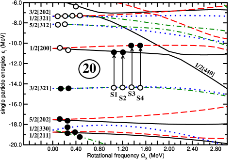
Figure 2: (Color online) Neutron single-particle energies (routhians) in the self-consistent rotating potential as a function of the rotational frequency $\Omega_{x}$. They are given along the deformation path of the yrast SD configuration in ⁴⁰Ca. Long-dashed, solid, dot-dashed and dotted lines indicate $(\pi=+,r=+i)$, $(\pi=+,r=-i)$, $(\pi=-,r=+i)$ and $(\pi=-,r=-i)$ orbitals, respectively. At $\Omega_{x}=0.0$ MeV, the single-particle orbitals are labeled by the asymptotic quantum numbers $[Nn_{z}\Lambda]\Omega$ (Nilsson quantum numbers) of the dominant component of the wave function. Solid (open) circles indicate the orbitals occupied (emptied). The arrows indicate the particle-hole excitations leading to excited SD configurations; for these configurations only the changes (as compared with yrast SD configuration) in the occupation of the orbitals are indicated in the figure.

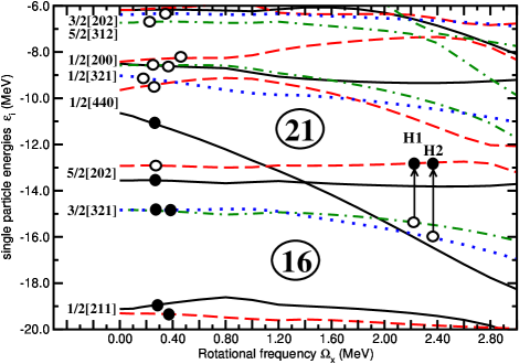
Figure 3: (Color online) The same as Fig. 2 but along the deformation path of the yrast HD configuration in ⁴⁰Ca. The arrows indicate the particle-hole excitations leading to excited HD configurations.

There are theoretical studies of deformed structures in these nuclei but they either focus on SD structures at high spin or are limited to a shape coexistence at low spin. For example, positive-parity states of ⁴⁰Ca were studied in Ref. Taniguchi et al. (2007) using antisymmetrized molecular dynamics (AMD) and the generator coordinate method (GCM); this is basically alpha-clustering model. The coexistence of low-spin normal- and superdeformed states in ³²S, ³⁶Ar, ³⁸Ar and ⁴⁰Ca has been studied in the GCM based on the Skyrme SLy6 functional in Ref. Bender et al. (2003). The SD and HD rotational bands in the $N=Z$ S, Ar, Ca, Ti and Cr nuclei have also been studied in cranked Hartree-Fock (CHF) approach based on the Skyrme forces in Refs. Yamagami and Matsuyanagi (2000); Inakura et al. (2002). A special attention has been paid to the SD structures in ³²S which were studied in detail in the CHF frameworks based on Skyrme Yamagami and Matsuyanagi (2000); Molique et al. (2000) and Gogny Rodríguez-Guzmán et al. (2000) forces and cranked relativistic mean field (CRMF) theory Afanasjev et al. (2000a). Exotic and highly-deformed $\alpha$-cluster configurations have been predicted long time ago in two-dimensional $\alpha$-cluster model in 4$N$ nuclei from ¹²C to ⁴⁴Ti in Ref. Zhang and Rae (1993). The investigation of superdeformation and clustering in these nuclei still remains an active field of research within the cluster models (see Refs. Kanada-En’yo and Kimura (2005); Maruhn et al. (2006); Taniguchi et al. (2007, 2010); Taniguchi (2014)).

There are several goals behind this study. First, it is imperative to understand at which spins extremely deformed configurations are expected to become yrast (or come close to the vicinity of the yrast line) and to find the best candidates for experimental studies of such structures. This requires detailed knowledge of terminating configurations up to their terminating states since they form the yrast line at low and medium spins. However, the tracing of terminating configurations from low spin up to their terminating states is non-trivial problem in density functional theories (see Sec. 8 in Ref. Vretenar et al. (2005) and Ref. Afanasjev (2008)). To our knowledge, such calculations have been done so far only in few nuclei: ²⁰Ne (in the cranked Skyrme HF Flocard et al. (1982) and CRMF Koepf and Ring (1989); Afanasjev and Abusara (2010a) frameworks), ⁴⁸Cr (in the HFB framework with Gogny forces Caurier et al. (1995)) and ¹⁰⁹Sb (in the CRMF framework Vretenar et al. (2005)). Note also that in ¹⁰⁹Sb they fail to reach the terminating state. With appropriate improvements in the CRMF computer code we are able to perform such calculations for the majority of the configurations forming the yrast line at low and medium spins. Second, the basic properties (such as transition quadrupole moments, dynamic and kinematic moments of inertia) of the configurations of interest, which could be compared in future with experimental data, are predicted. Third, we search for the fingerprints of the clusterization and molecular structures via a detailed analysis of the density distributions of the configurations under study.

The paper is organized as follows. Section II describes the details of the solutions of the cranked relativistic mean field equations. Detailed analysis of the structure of rotational spectra of ⁴⁰Ca and ⁴²Sc is presented in Secs. III and IV, respectively. A special attention is paid to the dependence of density distributions on the configuration. The general features of rotational spectra along the yrast line are discussed in Sec. V. Section VI is devoted to the discussion of the appearance of super-, hyper- and megadeformed configurations along the yrast line of the ^32,34S, ^36,38Ar, ^42,44Ca, ^44,46Ti and ^48,50Cr nuclei and their properties. The configurations which reveal the fingerprints of clusterization and molecular structures in their density distributions are discussed in Sec. VII. The kinematic and dynamic moments of inertia of selected SD, HD and MD configurations and their evolution with proton and neutron numbers and rotational frequency are considered in Sec. VIII. Finally, Section IX summarizes the results of our work.

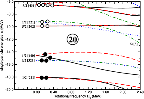
Figure 4: (Color online) The same as Fig. 2 but along the deformation path of the yrast MD [42,42] configuration in ⁴⁰Ca.

II The details of the theoretical calculations

In the relativistic mean-field (RMF) theory the nucleus is described as a system of pointlike nucleons, Dirac spinors, coupled to mesons and to the photons Serot and Walecka (1986); Reinhard (1989); Vretenar et al. (2005). The nucleons interact by the exchange of several mesons, namely a scalar meson $\sigma$ and three vector particles, $\omega$, $\rho$ and the photon. The CRMF theory Koepf and Ring (1989); König and Ring (1993); Afanasjev et al. (1996) is the extension of the RMF theory to the rotating frame in one-dimensional cranking approximation. It represents the realization of covariant density functional theory (CDFT) for rotating nuclei with no pairing correlations Vretenar et al. (2005). It has successfully been tested in a systematic way on the properties of different types of rotational bands in the regime of weak pairing such as normal-deformed Afanasjev and Frauendorf (2005), superdeformed Afanasjev et al. (1999b, 1996), as well as smooth terminating bands Vretenar et al. (2005) and the bands at the extremes of angular momentum Afanasjev et al. (2012).

The formalism and the applications of the CRMF theory to the description of rotating nuclei have recently been reviewed in Ref. Afanasjev (2016) (see also Refs. Vretenar et al. (2005); Afanasjev and Abdurazakov (2013)). A clear advantage of the CRMF framework for the description of rotating nuclei is the treatment of time-odd mean fields which are uniquely defined via the Lorentz covariance Afanasjev and Abusara (2010b); note that these fields substantially affect the properties of rotating nuclei Afanasjev and Ring (2000); Afanasjev and Abusara (2010a). Because the details of the CRMF framework could be found in earlier publications (Refs. Koepf and Ring (1989); König and Ring (1993); Afanasjev et al. (1996); Afanasjev and Abusara (2008)), we focus here on the features typical for the present study.

The pairing correlations are neglected in the present calculations. There are several reasons behind this choice. First, it is well known that pairing correlations are quenched by rotation (Coriolis anti-pairing effect) Ring and Schuck (1980); de Voigt et al. (1983). The presence of substantial shell gaps also leads to a quenching of pairing correlations Shimizu et al. (1989). Another mechanism of pairing quenching is blocking effect which is active in many nucleonic configurations Ring and Schuck (1980). In a given configuration, the pairing is also very weak at the spins close to band termination Afanasjev et al. (1999a). Moreover, the pairing drastically decreases after paired band crossings in the proton and neutron subsystems Afanasjev and Frauendorf (2005); at these spins the results of the calculations with and without pairing are very similar.

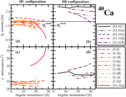
Figure 5: (Color online) Calculated transition quadrupole moments $Q_{t}$ and $\gamma$-deformations of the yrast and excited SD and HD configurations in ⁴⁰Ca. The colors of the lines for different types of configurations roughly correspond to those used in Fig. 1. Red and orange (black and dark brown) are used for the SD (HD) configurations.

Second, the calculations for blocked configurations within the cranked Relativistic Hartree-Bogoliubov (CRHB) framework Afanasjev et al. (2000b) are frequently numerically unstable Afanasjev and Abdurazakov (2013). This is a common problem for self-consistent Hartree-Bogoliubov or Hartree-Fock-Bogoliubov calculations which appears both in relativistic and non-relativistic frameworks Dobaczewski et al. (2015). On the contrary, these problems are much less frequent in unpaired CRMF calculations (see Ref. Afanasjev and Abusara (2008)). Even then it is not always possible to trace the configuration in the desired spin range. This typically takes place when (i) the local minimum is not deep enough for the solution (unconstrained in quadrupole moments) to stay in it during convergence process and (ii) occupied and unoccupied single-particle orbitals with the same quantum numbers come close in energy and start to interact.

Based on previous experience in ⁴⁰Ca (Ref. Ideguchi et al. (2001)), ⁴⁸Cr (Ref. Afanasjev et al. (1999a)) and somewhat heavier $N\sim Z$ $A=58-80$ nuclei (Refs. Afanasjev et al. (1999b); Afanasjev and Frauendorf (2005)), we estimate that the pairing becomes quite small and thus not very important above $I\sim 10\hbar$ in the nuclei of interest. This is exactly the spin range on which the current study is focused. Note also that the comparison of the CRHB and CRMF results for a few configurations in ⁴⁰Ca presented at the end of Sect. III supports this conclusion.

In the current study, we restrict ourselves to reflection symmetric shapes since previous calculations in the cranked Hartree-Fock approach with Skyrme forces Inakura et al. (2002) showed that odd-multipole (octupole, . . .) deformations play a very limited role in extremely deformed configurations of the mass region under study.

The CRMF equations are solved in the basis of an anisotropic three-dimensional harmonic oscillator in Cartesian coordinates characterized by the deformation parameters $\beta_{0}$ and $\gamma$ and oscillator frequency $\hbar\omega_{0}=41A^{−1/3}$ MeV, for details see Refs. Afanasjev et al. (1996); Koepf and Ring (1989). The truncation of basis is performed in such a way that all states belonging to the major shells up to $N_{F}=14$ fermionic shells for the Dirac spinors and up to $N_{B}=20$ bosonic shells for the meson fields are taken into account. This truncation scheme provides sufficient numerical accuracy (see Ref. Afanasjev and Abusara (2008) for details).

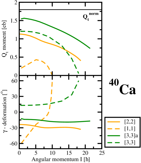
Figure 6: (Color online) The same as Fig. 5 but for the normal and highly-deformed triaxial configurations in ⁴⁰Ca.

The CRMF calculations have been performed with the NL3* functional Lalazissis et al. (2009) which is state-of-the-art functional for nonlinear meson-nucleon coupling model Agbemava et al. (2014). It is globally tested for ground state observables in even-even nuclei Agbemava et al. (2014) and systematically tested for physical observables related to excited states in heavy nuclei Afanasjev and Shawaqfeh (2011); Afanasjev and Abdurazakov (2013); Abusara et al. (2010). The CRMF and CRHB calculations with the NL3* CEDF provide a very successful description of different types of rotational bands Lalazissis et al. (2009); Afanasjev et al. (2012); Afanasjev and Abdurazakov (2013) both at low and high spins.

The quadrupole deformation $\beta_{2}$ is defined in self-consistent calculations from calculated quadrupole moments using the simple relation Afanasjev et al. (2003); Hilaire and Girod (2007); Samyn et al. (2005)

$$\beta_{2}=\frac{1}{XR^{2}}\sqrt{\frac{5\pi}{9}}Q^{X}_{0}$$ (1)

where $R=1.2A^{1/3}$ fm is the radius and $Q^{X}_{0}$ is a quadrupole moment of the $X$-th (sub)system expressed in fm². Here $X$ refers either to proton ($X=Z$) or neutron ($X=N$) subsystem or represents total nuclear system $(X=A)$. However this expression neglects the higher powers of $\beta_{2}$ and higher multipolarity deformations $\beta_{4}$, $\beta_{6}$,… Nazarewicz and Ragnarsson , which have an important role at very large deformations.

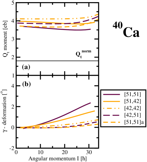
Figure 7: (Color online) The same as Fig. 5 but for the MD configurations in ⁴⁰Ca.

Because the definition of the deformation is model dependent Nazarewicz and Ragnarsson and deformation parameters are not experimentally measurable quantities, we prefer to use transition quadrupole moment $Q_{t}$ for the description of deformation properties of the SD, HD and MD bands. This is an experimentally measurable quantity and thus in future our predictions can be directly compared with the experimental results. The deformation properties of the yrast SD band in ⁴⁰Ca Ideguchi et al. (2001) are used as a reference. The measured transition quadrupole moment of this band is $Q^{exp}_{t}=1.8^{+0.35}_{-0.29}$ $e$b Ideguchi et al. (2001). Note that the CRMF calculations with the NL3* functional come close to experiment only slightly overestimating an experimental value (see Fig. 5 below). Thus we use $Q_{t}^{exp}=1.8$ $e$b in ⁴⁰Ca as a reference point. Note that the SD band in ⁴⁰Ca is the most deformed SD band among observed SD bands in this mass region.

Using this value we introduce the normalized transition quadrupole moment $Q_{t}^{norm}(Z,A)$ in the $(Z,A)$ system

$$Q^{norm}_{t}(Z,A)=\frac{ZA^{2/3}}{129.96}\,\,\,e{\rm b}$$ (2)

This is similar to what has been done in Ref. Afanasjev and Abusara (2008) in the analysis of the HD configurations in medium mass region. This equation is based on the ratio $Q_{t}^{norm}(Z,A)/Q_{t}(^{40}{\rm Ca})$ calculated using Eq. (1) under the assumption that the $\beta_{2}$ values in the $(Z,A)$ system and in ⁴⁰Ca are the same.

The band will be described as HD if its calculated $Q_{t}$ value exceeds $Q_{t}^{norm}(Z,A)$ by approximately 50%. This definition of HD is similar to the one employed in Ref. Afanasjev and Abusara (2008). Following suggestion of Ref. Dudek et al. (2004), we describe even more deformed bands as megadeformed. The band is classified as MD when its calculated $Q_{t}$ value is approximately twice of $Q_{t}^{norm}(Z,A)$ or higher.

Table 1: The semi-axis ratios of the density distributions of the indicated configurations. They are defined only for plotted density distrubutions (see, for example, Fig. 8). The semi-axis ratios are extracted at $\rho_{p}=0.04$ fm^-3 which roughly corresponds to a half of proton density in the central part of nucleus. The type of configuration (SD=superdeformed, HD=hyperdeformed and MD=megadeformed) is shown in column 3.

Nucleus	Configuration, spin	Type	Semi-axis ratio
1	2	3	4
40Ca	[4,4], $I=12$	SD	2.05
	[41,41], $I=24$	HD	2.27
	[42,42], $I=25$	MD	2.90
42Sc	[41,41], $I=22$	HD	2.23
	[52,52], $I=25$	MD	2.65
	[421,421], $I=31$	MD	3.40
	[421,421], $I=40$	MD	3.64
42Ca	[4,4]a, $I=21$	SD	2.17
	[62,42], $I=0$	MD	2.72
	[62,42], $I=16$	MD	2.79
44Ca	[62,42], $I=27$	MD	2.39
44Ti	[41,41], $I=25$	SD	2.03
	[62,62], $I=0$	MD	2.70
	[62,62], $I=32$	MD	2.88
46Ti	[62,51], $I=26$	SD	1.75
	[62,42], $I=28$	HD	2.40
48Cr	[62,62], $I=0$	HD	2.24
	[62,62], $I=28$	HD	2.39
50Cr	[62,62], $I=31$	HD	2.27
36Ar	[2,2], $I=4$	SD	1.9
	[4,4], $I=16$	HD	2.21
	[31,31], $I=21$	MD	2.56
	[41,41], $I=30$	MD	2.64
38Ar	[3,2]a, $I=12$	SD	1.91
	[42,31], $I=24$	HD	2.27
	[42,31], $I=32$	MD	2.74
32S	[2,2], $I=12$	SD	2.09
	[21,21], $I=31$	HD	2.15
34S	[2,1], $I=14$	SD	1.32
	[31,21], $I=21$	HD	2.32

Single-particle orbitals are labeled by $\Omega[Nn_{z}\Lambda](r=\pm i)$. $\Omega[Nn_{z}\Lambda]$ are the asymptotic quantum numbers (Nilsson quantum numbers) of the dominant component of the wave function at $\Omega_{x}=0.0$ MeV and $r$ is the signature of the orbital.

Because the pairing correlations are neglected, the intrinsic structure of the configurations of interest can be described by means of the dominant single-particle components of the intruder/hyperintruder/megaintruder states occupied. Thus, the calculated configurations will be labeled by shorthand [$n_{1}$($n_{2}$)($n_{3}$),$p_{1}$($p_{2}$)($p_{3}$)] labels, where $n_{1}$, $n_{2}$ and $n_{3}$ are the number of neutrons in the $N=3$, 4 and 5 intruder/hyperintruder/megaintruder orbitals and $p_{1}$, $p_{2}$ and $p_{3}$ are the number of protons in the $N=3$, 4 and 5 intruder/hyperintruder/megaintruder orbitals. The $N=5$ megaintruder orbitals are not occupied in the HD configurations. As a consequence, the labels $n_{3}$ and $p_{3}$ will be omitted in the labeling of such configurations. Moreover, the $N=4$ and $N=5$ orbitals are not occupied in the SD configurations. So, in those configurations the $n_{2}$, $n_{3}$ and $p_{2}$, $p_{3}$ labels will be omitted. An additional letter (a,b,c, …) at the end of the shorthand label is used to distinguish the configurations which have the same occupation of the intruder/hyperintruder/megaintruder orbitals (the same [$n_{1}$($n_{2}$)($n_{3}$),$p_{1}$($p_{2}$)($p_{3}$)] label) but differ in the occupation of non-intruder orbitals.

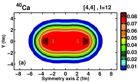
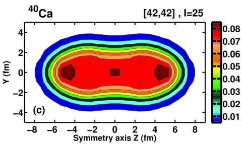
Figure 8: (Color online) The self-consistent proton density $\rho_{p}(y,z)$ as a function of $y$ and $z$ coordinates for the indicated configurations in ⁴⁰Ca at specified spin values. The equidensity lines are shown in steps of 0.01 fm^-3 starting from $\rho_{p}(y,z)=0.01$ fm^-3.

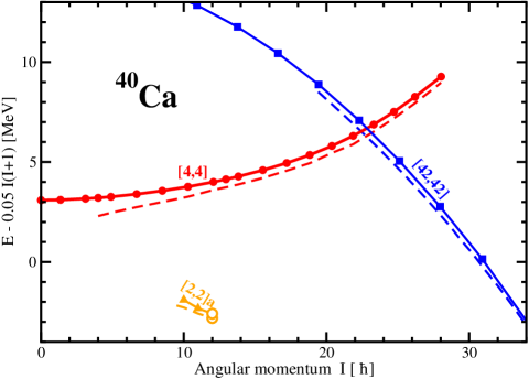
Figure 9: (Color online) The comparison of the results of the calculations with and without pairing for the configurations of ⁴⁰Ca which do not require blocking procedure in the CRHB calculations. The results of the calculations without pairing are shown by solid lines with symbols. The results for paired analogs of unpaired configurations are shown by dashed lines of the same color.

III The ⁴⁰Ca nucleus

⁴⁰Ca is a doubly magic spherical nucleus with 20 neutrons and 20 protons. Three lowest shells with $N=0$, 1 and 2 are occupied in its spherical ground state with $I=0^{+}$. Higher spin states are formed by particle-hole excitations from the $N=2$ shell into $f_{7/2}(N=3)$ subshell across the respective $Z=20$ and $N=20$ spherical shell gaps. This leads to a formation of complicated high-spin level scheme which includes spherical states and deformed, terminating and superdeformed rotational structures Ideguchi et al. (2001); Chiara et al. (2003); Caurier et al. (2007). In experiment, they extend up to spin $I=16^{+}$.

The results of the CRMF calculations for deformed configurations forming the yrast line are shown in Fig. 1. Different colors are used to indicate different classes of the bands. Note that low-spin spherical solutions are not shown here since we are interested in high-spin behavior of this nucleus.

The lowest deformed configuration [1,1] is based on simultaneous excitations of proton and neutron from the $d_{3/2}$ spherical subshell into the $f_{7/2}$ subshell across the $Z=20$ and $N=20$ spherical gaps. It has small quadrupole deformation of $\beta_{2}\sim 0.16$ and $\gamma\sim-24^{\circ}$ at $I=4\hbar$ and terminates at $I=10^{+}$ in a terminating state with the structure $\pi(f_{7/2})^{1}_{3.5}(d_{3/2})^{-1}_{1.5}\otimes\nu(f_{7/2})^{1}_{3.5}(d_{3/2})^{-1}_{1.5}$ and near-spherical shape. Additional excitations of the proton and neutron across the $Z=20$ and $N=20$ spherical gaps lead to a more deformed [2,2] configuration which has $\beta_{2}\sim 0.32$ and $\gamma\sim-30^{\circ}$ at $I=10\hbar$. It is expected to terminate at $I_{max}=20\hbar$ with the terminating state built at high energy cost and located high above the yrast line. However, we were not able to trace this configuration up to termination in the calculations. Next excitations of proton and neutron across the $Z=20$ and $N=20$ spherical gaps lead to even more deformed [3,3] configurations which are located close to each other up to spin $I=16\hbar$ (see Fig. 1). The configuration which terminates at spin $I=18\hbar$ is located in positive $\gamma$ minimum of potential energy surfaces and has $\beta_{2}\sim 0.47$ and $\gamma\sim 21^{\circ}$ at $I=12\hbar$. The structure of terminating state is $\pi(f_{7/2})^{3}_{7.5}(d_{3/2})^{-3}_{1.5}\otimes\nu(f_{7/2})^{3}_{7.5}(d_{3/2})^{-3}_{1.5}$. Another [3,3] configuration is located in the negative $\gamma$ minimum of potential energy surfaces and is expected to terminate at $I=24^{+}$. Similar to the [2,2] configuration we were not able to trace it up to terminating state which is expected to be located high above the yrast line.

Subsequent particle-hole excitations lead to an increase of the deformation of the configurations resulting in the formation of superdeformed rotational bands. Note that the bands with such deformation do not terminate in the single-particle terminating states (see Sec. 2.5 of Ref. Afanasjev et al. (1999a)). The yrast SD configuration [4,4] is characterized by large SD shell gap at particle number 20 both in the proton and neutron subsystems (Fig. 2). All single-particle states below these gaps are occupied in the [4,4] configuration. Note that apart of the Coulomb shift in energy the proton routhian diagram is similar to the neutron one shown in Fig. 2. The [4,4] configuration is only yrast at $I=22\hbar$; it is located above the yrast line at lower spin in agreement with the experiment Ideguchi et al. (2001). The accuracy of the description of the experimental data (dynamic and kinematic moments of inertia, transition quadrupole moments) is similar to the one obtained with the NL1 CEDF; the results obtained with this functional are compared with experiment in Ref. Ideguchi et al. (2001).

Starting from the yrast SD configuration [4,4] there are two ways to build excited configurations. The first one is by exciting particles from the $3/2[321](r=\pm i)$ orbitals into the $1/2[200](r=\pm i)$ orbitals; they are shown as the S1$-$S4 excitations in Fig. 2. The combination of proton and neutron excitations of this type leads to the [3,3] configurations. If the proton (neutron) excitations of this type are combined with the neutron (proton) configuration of the yrast SD band, the [3,4] and [4,3] configurations are created. These configurations are excited with respect to the yrast [4,4] SD configuration; some of them are shown by red lines in Fig. 1. Note that due to the similarity of the proton and neutron routhian diagrams some of these excited configurations are degenerated (or nearly degenerated) in energy. In addition, we show only some of highly excited SD configurations for the sake of clarity. An important feature is quite large energy gap between the yrast [4,4] and lowest excited [3,3]d SD configurations. Such a situation favors the observation of the yrast SD band since the feeding intensity is concentrated on it (see discussion in Refs. Afanasjev and Abusara (2008); Abusara and Afanasjev (2009)).

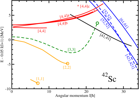
Figure 10: (Color online) The same as Fig. 1 but for ⁴²Sc.

Alternatively, one can excite the particle from either the $5/2[202](r=-i)$ or $5/2[202](r=+i)$ orbital to the lowest in energy hyperintruder $1/2[440](r=-i)$ orbital emerging from hyperintruder $N=4$ shell; the occupation corresponding to such a configuration is shown on left side of Fig. 3. The combination of the proton and neutron excitations of this kind leads to four-fold degenerate [41,41] HD configurations. This degeneracy is due to very small signature splitting of the configurations built on opposite signatures of the $5/2[202]$ orbitals and the combination of proton and neutron configurations of this kind.

At first glance this statement is in contradiction with Fig. 3 where there is a substantial energy splitting between the $r=-i$ and $r=+i$ branches of the $5/2[202]$ orbital which are almost parallel in rotational frequency. This feature is the consequence of non-pairwise occupation of the opposite signatures of some orbitals which leads to the presence of nucleonic currents at rotational frequency $\Omega_{x}=0.0$ MeV (see Sec. IVA in Ref. Afanasjev and Abusara (2010b)). The occupied orbital is always more bound than its unoccupied time-reversal counterpart. So the change of the signature of occupied $5/2[202]$ state (from $r=-i$ in Fig. 3 to $r=+i$) will only inverse the relative positions of both signatures of this orbital so that the total energy of the configurations built on the holes in the $5/2[202](r=-i)$ and $5/2[202](r=+i)$ orbitals will be almost the same.

The [41,41] configurations are the lowest in energy among the HD configurations at spins above $I=24\hbar$ (Fig. 1). The excited HD configurations [31,31]a and [31,31]b (Fig. 1) are formed as the combination of the H1 and H2 excitations (shown in Fig. 3) in the proton and neutron subsystems. The [31,41]a and [31,41]b configurations are based on the H1 and H2 excitations in the neutron subsystem and the proton configuration of the yrast [41,41] HD configuration. The [41,31]a and [41,31]b configurations (not shown in Fig. 1), based on the H1 and H2 excitations in the proton subsystem and the neutron configuration of the yrast [41,41] HD configuration, are located at the energies which are similar to the ones of the [31,41]a and [31,41]b configurations.

The HD configurations never become yrast in ⁴⁰Ca. However, such configurations compete with megadeformed ones for yrast status in neigbouring nuclei (see, for example, Secs. IV and VI.1). That was a reason for a quite detailed discussion of their structure.

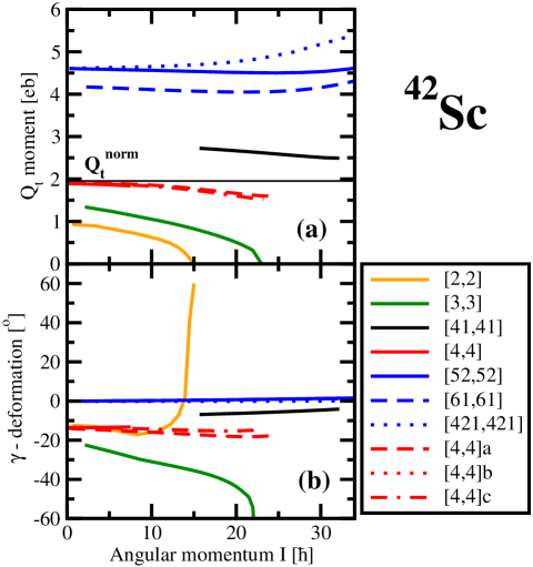
Figure 11: (Color online) The same as Fig. 5 but for ⁴²Sc.

The additional occupation of the $N=4$ proton and neutron orbitals leads to the [42,42] MD configuration which is yrast at spin above $I=23\hbar$ (Fig. 1). It is characterized by large (around 3 MeV) MD $Z=20$ and $N=20$ shell gaps (Fig. 4). Thus, this configuration can be considered as doubly magic megadeformed configuration. Indeed, excited MD configurations (such as [42,51], [51,51], [51,42] etc) are located at excitation energy of more than 2 MeV with respect to the yrast MD configuration (Fig. 1). The fact that the yrast MD configuration [42,42] is separated from the excited configurations by a such large energy gap should make its observation in experiment easier. This is because of the concentration of feeding intensity on the yrast MD configuration in such a situation (see discussion in Refs. Afanasjev and Abusara (2008); Abusara and Afanasjev (2009)).

Calculated transition quadrupole moments $Q_{t}$ and $\gamma$-deformations of the normal- and highly-deformed triaxial, SD, HD and MD configurations are shown in Figs. 5, 6 and 7. The configurations which are yrast in local deformation minimum, namely, SD [4,4], HD [41,41] and MD [42,42] have the largest transition quadrupole moment among the calculated SD, HD, and MD configurations, respectively. This is because particle-hole excitations leading to excited configurations reduce the number of occupied deformation driving orbitals.

Note that most of the calculated SD configurations have $\gamma\sim-12^{\circ}$. The only exception is the unusual [31,31]a configuration which has large positive $\gamma$-deformation rapidly increasing with spin. It has some similarities with the HD configurations. First, it involves the $N=4$ proton and neutron. Second, its slope in the $E-E_{RLD}$ plot is similar to the one of the HD configurations (see Fig. 1). However, it has substantially smaller $Q_{t}$ values as compared with the HD configurations.

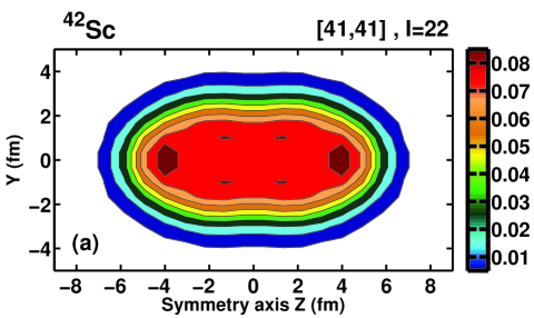
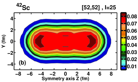
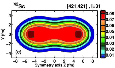
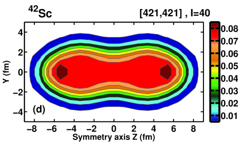
Figure 12: (Color online) The same as Fig. 8 but for ⁴²Sc.

While the calculated $Q_{t}$ and $\gamma$ values cluster for the SD configurations (Figs. 5a and c), they are scattered for the HD configurations (Figs. 5b and d). This suggests that the potential energy surfaces are much softer in the HD minimum as compared with the SD one. Indeed, in the HD minimum a single particle-hole excitation induces much larger changes in the $Q_{t}$ and $\gamma$ values than in the SD one. On the contrary, the MD configurations show the clusterization of the calculated $Q_{t}$ and $\gamma$ values which is similar to the one observed in the SD minimum (Fig. 7).

The most deformed HD configuration ([41,41]) has $Q_{t}$ values which are by roughly 40% larger than the ones for most deformed SD configuration ([4,4)]) (Fig. 5a and c). Yrast MD configuration [42,42] has the $Q_{t}$ values which are larger by roughly 45% and 105% than the ones for most deformed HD and SD configurations (compare Fig. 7a and Fig. 5a and c).

The self-consistent proton densities of the yrast SD, HD and MD configurations are shown in Fig. 8 at indicated spin values. The stretching of nuclear shape is definitely more pronounced in the HD [41,41] and especially in the MD [42,42] configurations. Indeed, the semi-major to semi-minor axis ratio is 2.05, 2.27 and 2.9 for the densities of the SD [4,4], HD [41,41] and MD [42,42] configurations. Note that the changes in the semi-axis ratio on going from one type of configurations to another are substantially smaller than relevant changes in the $Q_{t}$ values discussed above. The densities of the [41,41] HD configuration show some indications of the development of neck and these indications become much more pronounced in the MD [42,42] configuration.

Fig. 9 compares the results of the calculations with and without pairing for few selected configurations in ⁴⁰Ca. The calculations with pairing are performed in the cranked relativistic Hartree Bogoliubov (CRHB) framework of Ref. Afanasjev et al. (2000b). In these calculations the Lipkin-Nogami method is employed for an approximate particle number projection and the Gogny D1S force is used in pairing channel. The presence of pairing correlations leads to an additional binding. However, above $I=10\hbar$ this additional binding is rather modest (around 0.5 MeV or less) and it is similar for different calculated configurations. As a result, the general structure of the calculated configurations in the $E-E_{RLD}$ plot above this spin is only weakly affected by the presence of pairing. Similar effect has already been seen in the case of ⁷²Kr (Ref. Andreoiu et al. (2007)).

Note that among large number of the configurations obtained in unpaired calculations and presented in Fig. 1 only these three configurations (terminating [2,2]a, superdeformed [4,4] and hyperdeformed [42,42]), in which signature partner orbitals are pairwise occupied (see Figs. 2 and 4), can be calculated in the CRHB framework without blocking procedure. Particle-hole excitations leading to excited configurations remove pairwise occupation of the signature partner orbitals. As a result, the blocking procedure has to be employed for the calculation of such configurations in the CRHB framework. For example, the blocking of two particles is needed if the configuration label contains at least one odd number in either proton or neutron subsystem. If the configuration label contains odd number in both proton and neutron subsystems, then the blocking of four particles (two in proton subsystem and two in neutron subsystem) is needed. Such calculations are inherently unstable Afanasjev and Abdurazakov (2013); O’Leary et al. (2003). On the other hand, the blocking leads to an additional reduction of the impact of pairing correlations on physical observables (see Ref. Afanasjev and Abdurazakov (2013)). As a result, even smaller effect of pairing (as compared with the one shown in Fig. 9) is expected on binding energies of the configurations of Fig. 1 not shown in Fig. 9.

IV ⁴²Sc nucleus

⁴²Sc nucleus is formed by an addition of one proton and one neutron to ⁴⁰Ca. This is only odd-odd nucleus considered in the present paper. The configurations forming the yrast line of ⁴²Sc are shown in Fig. 10. The [1,1] configuration is built in valence space; it terminates at $I=7^{+}$. The [2,2] configuration is an analog of the [1,1] configuration in ⁴⁰Ca but with an extra proton and extra neutron placed into the orbitals emerging from the $f_{7/2}$ spherical subshell. As a consequence, it has substantially larger deformation and maximum spin within the configuration than the [1,1] configuration in ⁴⁰Ca. At spin $I=4\hbar$, the deformation of the [2,2] configuration is $\beta_{2}\sim 0.27$ and $\gamma\sim-15^{\circ}$. It terminates at $I=15^{+}$ in a terminating state with the structure $\pi(f_{7/2})^{2}_{6.0}(d_{3/2})^{-1}_{1.5}\otimes\nu(f_{7/2})^{2}_{6.0}(d_{3/2})^{-1}_{1.5}$ and near-spherical shape with $\beta_{2}\sim 0.05$.

Table 2: The maximum spin (in $\hbar$) which could be built within the configuration of given type. The asterisk is used to indicate the configurations which involve the hole(s) in the $d_{5/2}$ orbital(s). The SD configurations are not included into this table. See text for the discussion of the details.

Nucleus	valence space	2p-2h	4p-4h
1	2	3	4
40Ca	[0,0], $I_{max}=0$	[1,1], $I_{max}=10$	[2,2], $I_{max}=20$*
42Ca	[2,0], $I_{max}=6$	[3,1], $I_{max}=14$	[4,2], $I_{max}=24$*
44Ca	[4,0], $I_{max}=8$	[5,1], $I_{max}=14$	[6,2], $I_{max}=20$*
42Sc	[1,1], $I_{max}=7$	[2,2], $I_{max}=15$	[3,3], $I_{max}=23$*
44Ti	[2,2], $I_{max}=12$	[3,3], $I_{max}=18$	[4,4], $I_{max}=24$*
46Ti	[4,2], $I_{max}=14$	[5,3], $I_{max}=19$	[6,4], $I_{max}=22$*
48Cr	[4,4], $I_{max}=16$	[5,5], $I_{max}=20$*	[6,6], $I_{max}=20$*
50Cr	[6,4], $I_{max}=14$	[7,5], $I_{max}=16$*
36Ar	[0,0], $I_{max}=8$*	[1,1], $I_{max}=16$*
38Ar	[0,0], $I_{max}=4$*	[1,1], $I_{max}=14$*
32S	[0,0], $I_{max}=12$*	[1,1], $I_{max}=20$*
34S	[0,0], $I_{max}=10$*	[1,1], $I_{max}=19$*

Additional excitations of the proton and neutron across the $Z=20$ and $N=20$ spherical gaps lead to a more deformed [3,3] configuration which has $\beta_{2}\sim 0.37$ and $\gamma\sim-31^{\circ}$ at $I=10\hbar$. It is expected to terminate at $I_{max}=23\hbar$ with the terminating state built at high energy cost and located above the yrast line. However, we were able to trace this configuration in the calculations only up to $I\approx 22\hbar$ (one $\hbar$ short of termination).

The lowest four SD configurations [4,4] in ⁴²Sc are formed from the yrast SD configuration [4,4] in ⁴⁰Ca by addition of the proton and neutron to the $1/2[200](r=\pm i)$ orbitals located above the $Z=20$ and $N=20$ SD shell gaps (see Fig. 2). Their deformation properties are summarized in Fig. 11. Similar to the SD bands in ⁴⁰Ca, they are located in the $\gamma\sim-12^{\circ}$ minimum of potential energy surfaces. Note that the lowest [4,4] SD configuration undergoes unpaired band crossing (due to the crossing of the $1/2[400](r=-i)$ and $1/2[200](r=-i)$ orbitals seen in Fig. 2) which leads to the [41,41] HD configuration.

At spin above $I=22\hbar$, the HD configuration [41,41] becomes the lowest in energy. In this configuration, all single-particle states below the $Z=21$ and $N=21$ HD shell gap (Fig. 3) are occupied. So contrary to the yrast HD bands in ⁴⁰Ca, which are degenerate in energy, the yrast HD line in ⁴²Sc is represented by a single strongly decoupled branch of the [41,41] configuration.

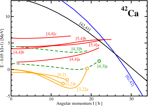
Figure 13: (Color online) The same as Fig. 1 but for ⁴²Ca.

At even higher spin (above $I=30\hbar$), the yrast line is formed by the megadeformed configuration [421,421] (Fig. 10). This configuration contains the proton and neutron in the lowest megaintruder $N=5$ orbital above the unpaired band crossing at $\Omega_{x}\sim 1.80$ MeV (above $I=31\hbar$). At lower spin the structure of this MD configuration is [52,52]; this is a result of unpaired band crossing emerging from the interaction of the lowest megaintruder $(N=5)(r=+i)$ orbital with the $1/2[321](r=+i)$ orbital taking place at $\Omega\sim 1.8$ MeV (Fig. 4). Note that this band crossing is blocked in the closely lying [52,52] MD configuration, shown by solid blue line in Fig. 10, in which the 21th proton and 21th neutron are placed into the $1/2[321](r=-i)$ orbital located above the $Z=20$ and $N=20$ MD shell gaps.

Proton density distributions for the HD configuration [41,41] and MD configurations [52,52] and [421,421] are shown in Fig. 12. The major semi-axis ratio of the proton density distribution increases only moderately (from 2.23 to 2.65 [see Table 1]) on going from the [41,41] configuration to the [52,52] one. However, this transition triggers drastic change in transition quadrupole moment $Q_{t}$; it is increased from $Q_{t}\sim 2.65$ $e$b for the [41,41] configuration to $Q_{t}\sim 4.5$ $e$b for the [52,52] configuration (see Fig. 11). The occupation of the megaintruder proton and neutron $N=5$ orbitals leading to the MD [421,421] configuration creates both additional elongation of the proton density and neck in this density distribution (see bottom panels of Fig. 12). The [421,421] configuration is the most elongated structure studied in the present paper. Three-dimensional representation of its density distribution is shown in Fig. 1a of Supplemental Material (Ref. Sup ). This density distribution has large semi-axis ratio of 3.40 at $I=31$ which is increasing with spin (Table 1). In part, this large value is a consequence of the development of the neck which leads to small semi-axis in the direction perpendicular to elongation. Note that despite large difference in the semi-axis ratio (3.40 for the [421,421] configuration and 2.65 for the [52,52] one), the $Q_{t}$ value of the [421,421] configuration ($Q_{t}\sim 5.2$ $e$b at $I=31\hbar$) is only by 15% larger that the one for the [52,52] configuration (see Fig. 11). These examples clearly indicate that there is no simple relation between the semi-axis ratio of the proton density distribution and transition quadrupole moments.

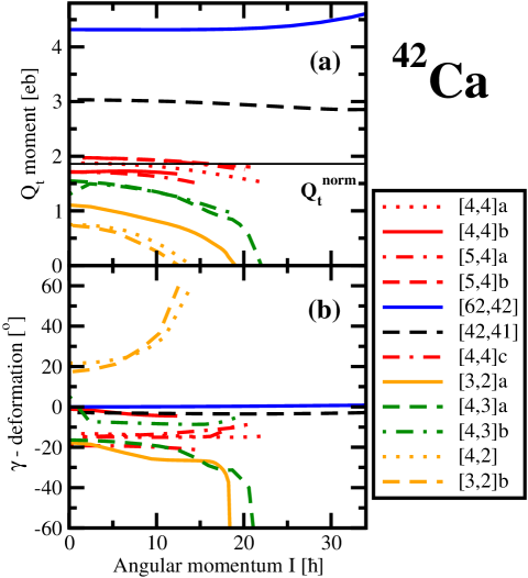
Figure 14: (Color online) The same as Fig. 5 but for ⁴²Ca.

V The general features of high-spin spectra

The discussion of low-spin spectra in Secs. III and IV clearly shows the importance of particle-hole excitations across the $N=20$ and $Z=20$ spherical shell gaps in building angular momentum and deformation. The most striking example is ⁴⁰Ca in which only the ground state could be built in the valence space. Here the valence space is defined as the configuration space which does not involve particle-hole excitations across either the $N=20$ and $Z=20$ spherical shell gaps or the $N=28$ and $Z=28$ spherical shell gaps.

The maximum spin which could be built in the valence space of nuclei is summarized in Table 2. It is defined with respect of spherical ⁴⁰Ca core by the occupation of proton and neutron $f_{7/2}$ orbitals in the Ca, Sc, Ti and Cr nuclei and by the proton and neutron holes in the $N=2$ $d_{3/2}$, $s_{1/2}$ and $d_{5/2}$ orbitals in the Ar and S nuclei. One can see that the maximum spin increases on approaching the middle of the $f_{7/2}$ subshell where it reaches the maximum value of $I_{max}=16\hbar$ in the $\pi(f_{7/2})^{4}_{8.0}\otimes\nu(f_{7/2})^{4}_{8.0}$ configuration of ⁴⁸Cr. Note that the addition of two neutrons to this configuration decreases the maximum spin which could be built in the valence space of ⁵⁰Cr (see Table 2).

Table 2 also illustrates how the maximum spin, which could be built within the configuration, changes when particle-hole excitations across the spherical $Z=20$ and $N=20$ spherical shell gaps are involved. Here 2p-2h configurations are defined as the configurations which involve the excitations of one proton and one neutron across the respective shell gaps. The excitations of two protons and two neutrons across these gaps lead to the 4p-4h configurations. The impact of these excitations on the maximum spin depend on how many occupied $f_{7/2}$ orbitals in the Ca, Sc, Ti and Cr nuclei (or holes in the $N=2$ orbitals of the Ar and S nuclei) the nucleus has in its valence space. One can see that these excitations increase drastically the maximum spin within the configurations of ⁴⁰Ca but have limited impact on maximum spin in ⁴⁸Cr (Table 2).

The analysis of the ⁴⁰Ca and ⁴²Sc nuclei clearly indicates that subsequent particle-hole excitations lead to the yrast or near-yrast SD, HD and MD configurations at the spins which are either similar to the maximum spins which could be built within the 2p-2h and 4p-4h configurations or slightly above them. Note that the nuclei in these 2p-2h and 4p-4h configurations could at most be described as highly-deformed.

The importance of these 2p-2h and 4p-4h configurations lies in the fact that at low and medium spins they dominate the yrast line and thus are expected to be populated in experiment with high intensity. The observation of the SD, HD and MD configurations requires that these bands are either yrast or close to yrast at the spins where the feeding of the bands takes place. This is especially critical for the HD and MD bands since in most of the nuclei they have completely different slope in the $E-E_{RLD}$ plots as compared with the bands of smaller deformation. As a result, their excitation energies with respect to the yrast line grow up very rapidly with decreasing spin below the spins where the HD and MD bands are yrast or near yrast. This factor will limit the spin range in which they can be observed in future experiments to the spin range in which these bands are either yrast or close to yrast and few states below this spin range.

Considering the limitations of experimental facilities to observe high spin states in light nuclei, it is imperative that expected candidates for the SD, HD and MD bands become yrast (or close to yrast) at the spins which are not far away from currently measured. Indeed, with current generation of detectors the SD bands in ³⁶Ar Svensson et al. (2000) and ⁴⁰Ca Ideguchi et al. (2001) and ground state band in ⁴⁸Cr Brandolini et al. (1998) are observed up to $I=16\hbar$ which represents the highest spin measured in this mass region. The advent of $\gamma$-tracking detectors such as GRETA and AGATA will increase the spin up to which the measurements could be performed but this increment in spin is not expected to be drastic.

Note that the results discussed in this section only illustrate the general features of rotating nuclei and provide some crude estimates of the competition of terminating and extremely deformed configurations. Indeed, detailed calculations are needed to define the properties of such bands and the spins at which extremely deformed configurations become yrast. For the sake of simplicity, we also do not discuss here possible excitations across the spherical $N=28$ and $Z=28$ shell gaps. Terminating configurations based on such excitations compete with the SD, HD and MD configurations only in ⁴⁶Ti and Cr nuclei (see Secs. VI.4, VI.5 and VI.6 below).

The examples of the ⁴⁰Ca and ⁴²Sc nuclei discussed above once more confirm that rotating nuclei are the best laboratories to study the shape coexistence. Indeed, starting from either spherical or weakly deformed ground states by means of subsequent particle-hole excitations one can built any shape (prolate, oblate, triaxial, super-, hyper- and megadeformed as well as cluster and/or molecular structures [see Sec. VII below for a discussion of latter structures/shapes]) in the same nucleus.

VI Other nuclei in the neigbourhood of ⁴⁰Ca

The results for other nuclei studied in this paper will be presented in this section. In the calculations of terminating structures at low and medium spins we concentrate on the configurations which define the general structure of the yrast line and the spins at which the transition to extremely deformed configurations takes place. Apart from few interesting cases, we do not discuss them in detail. The main focus of this section is on the super-, hyper- and megadeformed rotational configurations and, in particular, on the ones which potentially show the features of clusterization and molecular structures. In order to provide the guidance for future experiments, we present the $(E-E_{RLD})$ plots and the figures with transition quadrupole moments and $\gamma$-deformations for each nucleus. In addition, the proton density plots are provided for the yrast or near-yrast configurations which could be measured in future experiments. The goals behind that is to see the evolution of the density distribution with configuration and nucleus and to find interesting candidates for clusterization and molecular structures. Note that some graphical results of the calculations are provided in the Supplemental Material with this article as Ref. Sup .

VI.1 ⁴²Ca nucleus

The energies of calculated configurations are shown in Fig. 13. The calculated transition quadrupole moments and $\gamma$-deformations of these configurations are displayed in Fig. 14. Note that this nucleus has two extra neutrons as compared with ⁴⁰Ca which affects the structure of the configurations.

The SD configurations are represented by the [4,4]a, [4,4]b, [4,4]c, [5,4]a and [5,4]b configurations (Fig. 13). The yrast [4,4]a SD configuration in ⁴²Ca is formed by an addition of two extra neutrons in the 1/2[200] orbitals (located above the $N=20$ SD shell gap [Fig. 2]) to the yrast [4,4] SD configuration of ⁴⁰Ca. Note that similar to ⁴⁰Ca the SD configurations in ⁴²Ca are triaxial with $\gamma\sim-12^{\circ}$.

At spin $I\sim 23\hbar$, the expected continuation of the SD [4,4] configuration is crossed by the HD [42,41] configuration which is formed from the yrast HD [41,41] configuration in ⁴⁰Ca (Fig. 3) by adding one neutron into the $1/2[440](r=+i)$ orbital and another into the $5/2[202](r=+i)$ orbital. The HD [42,41] configuration has near prolate shape with $Q_{t}$ value which exceed by 50% the $Q_{t}$ values which are typical for the SD bands (Fig. 14).

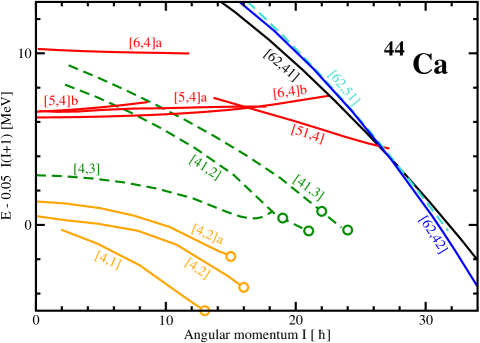
Figure 15: (Color online) The same as Fig. 1 but for ⁴⁴Ca. Note that for some configurations several aligned (terminating) states can be formed; the reasons for their formation are discussed in Sec. 6.6 of Ref. Afanasjev et al. (1999a).

Axially symmetric MD configuration [62,42] becomes yrast above $I=26\hbar$ (Fig. 13). At these spins, its transition quadrupole moment is by $\sim 50\%$ larger than that of the HD [42,41] configuration (Fig. 14).

Proton density distributions of the yrast SD [4,4]a and MD [62,42] configurations are shown in Fig. 2a of supplemental material (Ref. Sup ) and Figs. 33c and d below, respectively. The major semi-axis ratio is 2.17 and 2.79 for these configurations (Table 1). However, the $Q_{t}$ values of the latter configuration are by a factor of more than 2 larger than those of the former one (Fig. 14).

VI.2 The ⁴⁴Ca nucleus

The SD configurations are represented by the [6,4] and [51,4] configurations (Fig. 15). However, up to spin $I\sim 22\hbar$ the total yrast line is formed by the normal- and highly-deformed triaxial terminating configurations and these SD configurations are located at high excitation energy with respect to the total yrast line. Only around $I\sim 24\hbar$, the [51,4] SD configuration becomes yrast. However, already at spin $I=26\hbar$ and above the yrast line is formed by closely lying [62,41] HD and [62,42] MD configurations.

The calculated values of the transition quadrupole moment $Q_{t}$ of these configurations are shown in Fig. 3 of supplemental material (Ref. Sup ). Proton density distribution of the MD [62,42] configuration is displayed in Fig. 2b in the supplement to present paper (Ref. Sup ). The [62,51] configuration, shown by dashed cyan line in Fig. 15, is lying closely in energy to these two configurations. Its calculated $Q_{t}$ values are in the between the ones for the HD and MD configurations (see Fig. 3 in the supplement).

The yrast line of ⁴⁴Ca shows that with increasing neutron number up to $N=24$ (which leads to the placement of the neutron Fermi level in the middle of deformed single-particle states emerging from spherical $1f_{7/2}$ subshell) it become energetically favorable to excite the neutron across the spherical $N=28$ shell gap. Such excitation leads to the occupation of the lowest $1g_{9/2}$ neutron orbital (which carries substantial single-particle angular momentum) and, in the case of ⁴⁴Ca, to the formation of the [41,2] and [41,3] configurations which terminate at spins $I=21,22$ and 24$\hbar$ (Fig. 15). As a consequence, the yrast line could be built by either normal- or highly-deformed terminating configurations up to higher spins in ⁴⁴Ca as compared with lighter Ca isotopes (compare Figs. 15, 13 and 1). As a result, the observation of the SD, HD and MD configurations would be more difficult in heavier Ca isotopes as compared with ⁴⁰Ca. Note that this mechanism of neutron excitations across the $N=28$ spherical shell gap affects also the yrast line in ⁴⁶Ti (configuration [41,4], Fig. 18). Similar proton excitation across the $Z=28$ spherical shell gap become active in the Cr isotopes. Indeed the configurations of the type [*1,*1] built on simultaneous neutron and proton excitations across the $N=28$ and $Z=28$ spherical shell gaps are active in the creation of the yrast line at medium spin in ^48,50Cr (see Figs. 20 and 21 below).

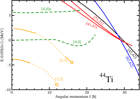
Figure 16: (Color online) The same as Fig. 1 but for ⁴⁴Ti. Note that is was not possible to trace the middle parts of the [2,2] and [3,3] configurations in the calculations. Thus, they are shown by dotted lines.

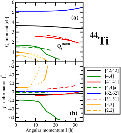
Figure 17: (Color online) The same as Fig. 5 but for ⁴⁴Ti.

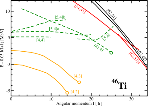
Figure 18: (Color online) The same as Fig. 1 but for ⁴⁶Ti.

VI.3 The ⁴⁴Ti nucleus

The SD configurations are represented by the [41,41] and [51,51] configurations (see Figs. 16 and 17). These configurations are either yrast or very close to yrast line above $I=24\hbar$ after the crossing with expected continuation of the [4,4] configuration. The [4,4] and [4,4]a configurations may also be considered as SD at low spin since they are located at the borderline between the SD and highly-deformed bands. The increase of the proton and neutron numbers to 22 leads to a decrease of the impact of the hyperintruder $N=4$ orbitals. Indeed, the [41,41] and [51,51] configurations have transition quadrupole moments $Q_{t}$ which are only slightly above the one typical for the SD configurations (Fig. 17).

Only the occupation of additional proton and neutron $N=4$ hyperintruder orbitals leads to the configuration [42,42] (see Fig. 16) which is truly hyperdeformed (Fig. 17). However, the HD configurations are never yrast in this nucleus. At spin $I\sim 29\hbar$, the MD [62,62] configuration becomes yrast. Proton density distribution of this configuration (see Figs. 33e and f below) could be compared with the one for the SD [41,41] configuration (see Fig. 2c in the supplemental material (Ref. Sup )). Its three dimensional representation is shown in Fig. 1b of the supplement to this manuscript. The $Q_{t}$ value of the MD configuration is larger than the one for the SD configuration by a factor of approximately 2.5 (Fig. 17). On the other hand, the difference in the ratio of major semi-axis of the density distribution of these two configurations is smaller (the major semi-axis ratio is 2.88 for the [62,62] configuration and 2.03 for the [42,42] configuration [Table 1]).

VI.4 The ⁴⁶Ti nucleus

As discussed in Sec. VI.2, the increase of neutron number to $N=24$ leads to a situation in which the particle-hole excitations across the $N=28$ spherical shell gap create the configurations which contribute to the yrast line at medium spin (the [4,4] configuration terminating at $I=25\hbar$, Fig. 18). At higher spin the SD [62,51]a configuration becomes yrast. The HD [62,42] configuration is only slightly excited in energy with respect to this configuration. Proton density distributions of these two configurations are shown in Figs. 2d and e of supplemental material (Ref. Sup ). Note that the MD configurations are not energetically favored in this nucleus and they do not show up in the vicinity of the yrast line in the spin range of interest. The calculated $Q_{t}$ and $\gamma$-deformation values of the configurations displayed in Fig. 18 are summarized in Fig. 19.

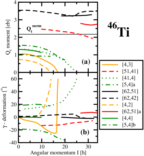
Figure 19: (Color online) The same as Fig. 5 but for ⁴⁶Ti.

VI.5 ⁴⁸Cr nucleus

The valence space terminating [4,4] configuration is forming the yrast line up to $I=16\hbar$ (Fig. 20). This band has been observed in experiment up to its termination in Ref. Brandolini et al. (1998). Particle-hole excitations across the $Z=20$ and $N=20$ spherical shell gaps lead to only marginal increase of angular momentum content of the configurations but cost a lot of energy (see, for example, the configurations [4,5] and [5,5] in Fig. 20 and Table 2). Higher spin configurations are built at a reasonable energy cost by particle-hole excitations across the $Z=28$ and $N=28$ spherical shell gaps. Such excitations lead both to terminating and SD/HD configurations. The first type of configurations is represented by the [41,41] one which terminates at $I=30\hbar$. The SD [52,52] and HD [62,62] configurations lying at similar energies become the lowest configurations at spin $I\geq 30\hbar$ (Fig. 20). Note that the resonance observed at $I\sim 36\hbar$ in the ²⁴Mg+²⁴Mg reaction strongly supports a HD shape for a compound ⁴⁸Cr nucleus formed in this reaction Di Nitto et al. (2016). The evolution of proton density distribution with spin in the [62,62] configuration is shown in Figs. 2f and g of the supplemental material (Ref. Sup ). The $Q_{t}$ and $\gamma$-deformation values are summarized in Fig. 5 of the supplemental material.

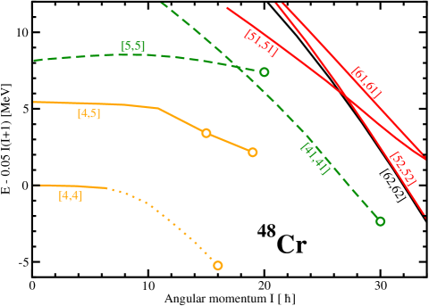
Figure 20: (Color online) The same as Fig. 1 but for ⁴⁸Cr.

VI.6 ⁵⁰Cr nucleus

The calculated configurations are shown in Fig. 21. Below spin $I=14\hbar$, the yrast line is built from valence space [6,4] configuration. Higher spin terminating configurations ([51,4], [51,31] and [51,41]) are build by means of particle-hole excitations across the $Z=28$ and $N=28$ spherical shell gaps. They dominate the yrast line up to $I=31\hbar$. At even higher spin closely lying HD [62,62] and [72,62] configurations are either yrast or close to yrast. Transition quadrupole moments $Q_{t}$ and $\gamma$-deformations of the calculated configurations are summarized in Fig. 6 of the supplemental material (Ref. Sup ). An example of proton density distribution is shown in Fig. 2h of the supplemental material for the HD [62,62] configuration at $I=31\hbar$. Note that neither superdeformed nor megadeformed configurations show up in the vicinity of the yrast line in this nucleus in the spin range of interest.

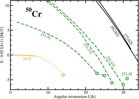
Figure 21: (Color online) The same as Fig. 1 but for ⁵⁰Cr.

VI.7 ³⁶Ar nucleus

The maximum spin which could be built in the valence space of this nucleus is quite limited, namely, $8\hbar$ in the [0,0] configuration (Fig. 22 and Table 2). Particle-hole excitations leading to the [1,1] configurations increase this spin up to $16\hbar$ (configuration [1,1]a in Fig. 22). Subsequent particle-hole excitations generate the [2,2] configurations the maximum spin within which is $20\hbar$ (see Table 2).

One of such configurations terminating at $I=16\hbar$ is assigned to the SD band observed in Refs. Svensson et al. (2000, 2001). Its properties have been studied earlier within the spherical shell model Caurier et al. (2005) and cranked Nilsson-Strutinsky approach Svensson et al. (2000, 2001). Based on the calculated deformation properties, this configuration could be considered as SD only at low spin. This is because with increasing spin its transition quadrupole moment $Q_{t}$ is decreasing rapidly and $\gamma$-deformation is increasing up to $\gamma=60^{\circ}$ (Fig. 23). Terminating state of this configuration/band is reached at $I=16^{+}$ both in theory (Fig. 22) and in experiment (Refs. Svensson et al. (2000, 2001)). From our point of view, the classification of this band as highly-deformed triaxial is more appropriate but we label it as SD in Fig. 1 following the classification established in the literature.

At spin above $I=16\hbar$, the yrast line is built from the HD [4,4] and MD [31,31] configurations. It is easy to understand the structure of these configurations from the routhian plot for the [42,42] MD configuration in ⁴⁰Ca (Fig. 4). The [4,4] configuration in ³⁶Ar is built by removing two protons and two neutrons in the $N=4$ orbitals from the MD [42,42] configuration in ⁴⁰Ca. The [31,31] configurations in ³⁶Ar are built by removing one proton and one neutron in the $N=4$ orbital from the [42,42] configuration in ⁴⁰Ca and another proton and another neutron from the $3/2[321]$ orbital of the same configuration. Since opposite signature branches of the $3/2[321]$ orbital are either degenerate in energy (as in Fig. 4) or have very small energy splitting, four [31,31] configurations are calculated at close energies. For simplicity, we show only the lowest one in Fig. 22.

Note that in many calculations these extremely deformed structures do not form a stable minimum in the potential energy surfaces at spin zero (see, for example, Fig. 2 in Ref. Ebran et al. (2014)). Thus, the rotation helps to stabilize this minimum. This is similar to the situation with the stabilization of hyperdeformation at high spin in medium mass nuclei (Ref. Afanasjev and Abusara (2008)).

The transition quadrupole moments $Q_{t}$ and $\gamma$-deformations of the calculated configurations are summarized in Fig. 23. One can see that the $Q_{t}$ values of the [4,4] and [31,31] MD configurations are by approximately 66% and 100% larger than the normalized transition quadrupole moment $Q_{t}^{norm}$ for the SD shapes. Proton density distributions of the SD [2,2] (at low spin), HD [4,4] and MD [31,31] and [41,41] configurations are shown in Fig. 24 (see also Table 1 for the density semi-axis ratios). Three-dimensional representation of the proton density distribution in the MD [31,31] configuration is shown in Fig. 1c of the supplemental material (Ref. Sup ). The SD shapes are characterized by more compact (with higher average density in the interior of the nucleus) density distribution as compared with the HD and MD shapes (Fig. 24). The formation of the necking degree of freedom is clearly seen in the MD [31,31] and [41,41] configurations.

The results obtained in the cranked Nilsson-Strutinsky (CNS) approach are very similar to the CRMF ones (see Fig. 6 in Ref. Afanasjev et al. (2000a)). Indeed, the MD [31,31] configurations are yrast above spin $I=18\hbar$ also in the CNS calculations. Considering that both experimental data in this nucleus extends up to $I=16^{+}$ and yrast or near yrast higher spin configurations are formed from HD and/or MD ones, the calculations in the CRMF and CNS frameworks clearly indicate this nucleus as one of the best candidates for the observation of the hyper- and megadeformations. In simple words, if it will be possible to bring higher (than $16\hbar$) angular momentum into this system, the population of the HD and MD states is the most likely outcome of this process.

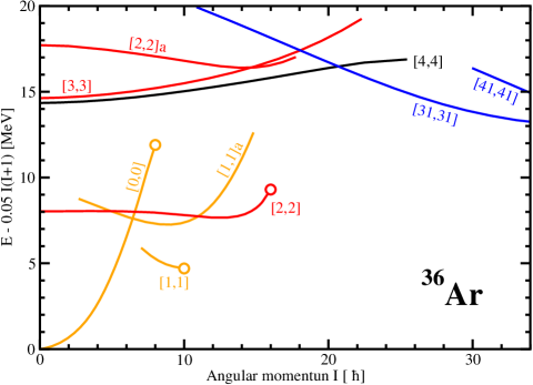
Figure 22: (Color online) The same as Fig. 1 but for ³⁶Ar.

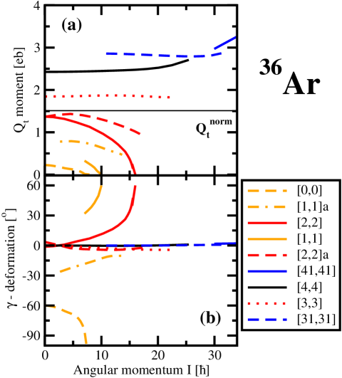
Figure 23: (Color online) The same as Fig. 5 but for ³⁶Ar.

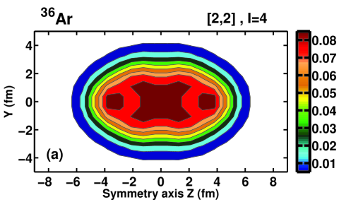
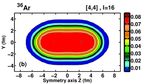
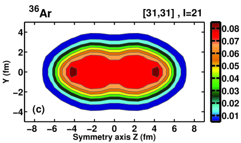
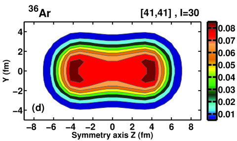
Figure 24: (Color online) The same as Fig. 8 but for ³⁶Ar.

VI.8 ³⁸Ar nucleus

Low-spin yrast line in this nucleus is built from terminating configurations (Fig. 25). The lowest SD configuration [3,2]a is close to the yrast line at medium spin and it becomes yrast above $I=17\hbar$ (Fig. 25). Similar to the observed SD band in ³⁶Ar, it terminates in non-collective state but at higher spin of $I=22\hbar$. Its proton density distribution at the medium spin of $I=12\hbar$ is shown in Fig. 3a of the supplemental material (Ref. Sup ). The yrast line above $I=22\hbar$ is built from the [42,31] MD signature partner configurations with small energy splitting (Fig. 25). They differ in the occupation by third proton of different signatures of the 3/2[321] orbital; there is almost no signature splitting between the different signatures of this orbital (see Fig. 4). An interesting feature of this configuration is substantial impact of rotation on the density distribution leading to a larger elongation and more pronounced necking with increasing spin from $I=24\hbar$ to $I=32\hbar$ (see Figs. 33a and b below). This however is not associated with the substantial change of transition quadrupole moment $Q_{t}$ (Fig. 26).

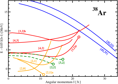
Figure 25: (Color online) The same as Fig. 1 but for ³⁸Ar.

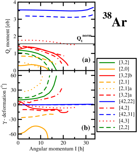
Figure 26: (Color online) The same as Fig. 5 but for ³⁸Ar.

VI.9 ³²S nucleus

The SD configurations were predicted in ³²S long time ago in Refs. Sheline et al. (1972); Leander and Larsson (1975). The SD bands built on such structures have been studied both in non-relativistic cranked DFTs based on the Gogny Tanaka et al. (2001); Rodríguez-Guzmán et al. (2000) and Skyrme Yamagami and Matsuyanagi (2000); Molique et al. (2000) forces and in the CRMF calculations with the NL3 CEDF in Ref. Afanasjev et al. (2000a). The detailed structure of the yrast spectra of this nucleus has also been investigated in the cranked Nilsson-Strutinsky (CNS) approach in Ref. Afanasjev et al. (2000a). Note that contrary to more microscopic studies which are limited to collective structures, this CNS study considers also terminating/aligned states along the yrast line which is important for a proper description of the yrast line at low and medium spins.

Fig. 27 shows the high-spin structures in ³²S. The lowest SD configuration with the structure [2,2] is yrast above spin $I=10\hbar$. The same result has also been obtained in other models quoted above. Above spin $I=24\hbar$, the occupation of the lowest $N=4$ hyperintruder proton and neutron orbitals leads to the HD [21,21] configuration. Note that this induces an unpaired band crossing the consequence of which is the impossibility to trace in the calculations the SD band above $I\sim 23\hbar$ and HD band below $I\sim 27\hbar$. This problem could be avoided if diabatic orbitals would be built using an approach of Ref. Afanasjev et al. (1999a); the expected diabatic continuations of the SD [2,2] and HD configurations [21,21] are shown by dotted lines in Fig. 27. Note that the CNS calculations of Ref. Afanasjev et al. (2000a) also suggest that the lowest HD configuration has the [21,21] structure and becomes yrast at similar spins. The same HD configuration has also been obtained in cranked Skyrme HF calculations of Ref. Yamagami and Matsuyanagi (2000); it also become yrast around $I\sim 25\hbar$ in the calculations with SIII and SkM* Skyrme forces.

At spin $I=0$, the calculated $Q_{t}$ values for the [2,2] SD configuration are 50% larger than $Q_{t}^{norm}$ (Fig. 28). This would even allow to describe this band as HD. However, at this spin the [2,2] SD configuration is located around 10 MeV above the ground state which prevents its observation. The rotation and the limited angular momentum content in low deformation configurations brings this SD configuration to the yrast line. However, it also triggers the decrease of the collectivity (as measured by $Q_{t}$) so this configuration is more properly described as SD in the spin range where it is yrast. The occupation of the lowest $N=4$ proton and neutron orbitals leading to the [21,21] HD configuration triggers substantial increase of $Q_{t}$; at spin $I=31\hbar$ it is by 60% larger than the $Q_{t}^{norm}$. Density distributions of the [2,2] and [21,21] configurations at spins of interest are shown in Fig. 29. Note that many [1,1] configurations are of transitional type; they are SD only at very low spins (Fig. 28) and are only highly-deformed at higher spins. Truly SD configurations are obtained with additional occupation of the $N=3$ orbital leading to either [2,1] or [1,2] configurations (Fig. 28).

Present calculations indicate large gap between the yrast SD [2,2] configuration and excited configurations in the spin range $I=16-22\hbar$ (Fig. 27). Although this would favor the population of this configuration, all experimental attempts to observe this band undertaken in the beginning of the last decade have failed.

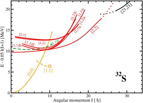
Figure 27: (Color online) The same as Fig. 1 but for ³²S. Dotted lines show expected diabatic continuations of the [2,2] and [21,21] configurations beyond the spin range where the convergence has been obtained.

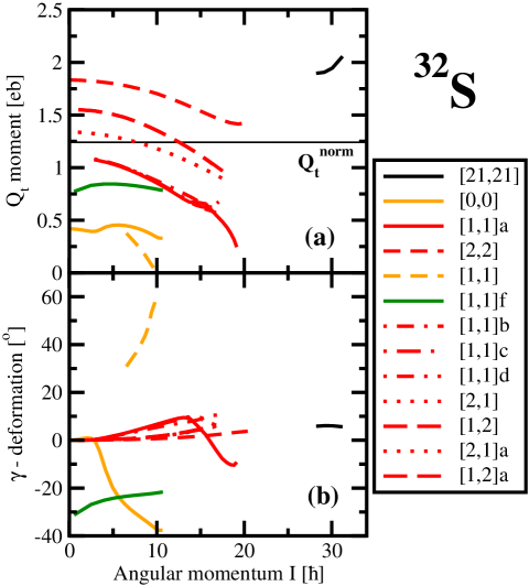
Figure 28: (Color online) The same as Fig. 5 but for ³²S.

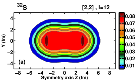
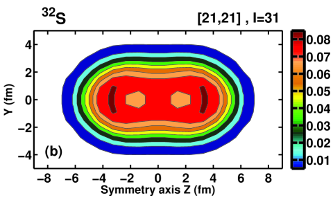
Figure 29: (Color online) The same as Fig. 8 but for ³²S.

VI.10 ³⁴S nucleus

The configurations in the ³⁴S nucleus are formed from the ones in ³²S by adding two neutrons in respective orbitals. The [2,1] configurations in ³⁴S are similar to the [1,1] ones in ³²S; they are SD at low spin but lose the collectivity with increasing spin so that they are better described as highly-deformed at the highest calculated spins (Fig. 31). Indeed, their density distributions at medium and high spins are characterized by rather modest semi-axis ratio; this is seen in Fig. 3b of the supplemental material (Ref. Sup ) on the example of the [2,1] configuration which has semi-axis ratio of 1.32 (see Table 1) at $I=14\hbar$. Similar to ³²S truly SD shapes are formed with the occupation of at least two $N=3$ protons and two $N=3$ neutrons. They are represented by the [2,2] SD configuration (which is yrast above $I=16\hbar$ [see Fig. 30]) and by the excited [3,2] and [3,2]a SD configurations. The occupation of the lowest $N=4$ neutron and proton orbitals leads to the HD configurations [31,21] and [31,11]. The first configuration is yrast at spin $I=20\hbar$ and above (Fig. 30) and its proton density distribution is shown in Fig. 32.

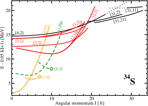
Figure 30: (Color online) The same as Fig. 1 but for ³⁴S.

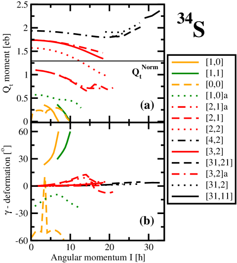
Figure 31: (Color online) The same as Fig. 5 but for ³⁴S.

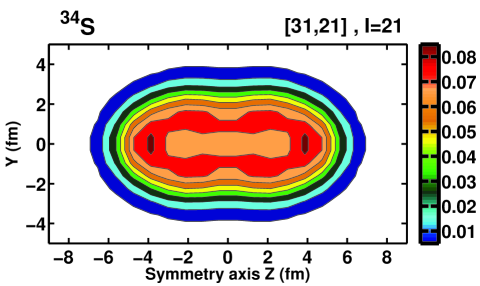
Figure 32: (Color online) The same as Fig. 8 but for ³⁴S.

VII Clusterization and molecular structures

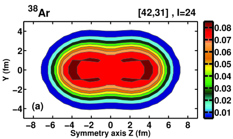
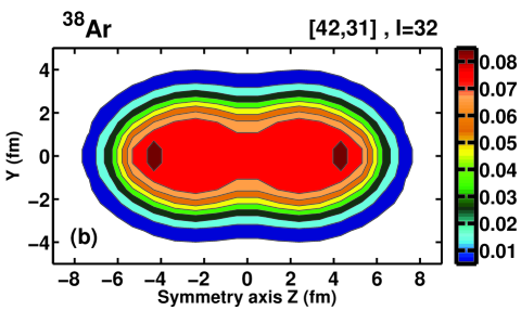
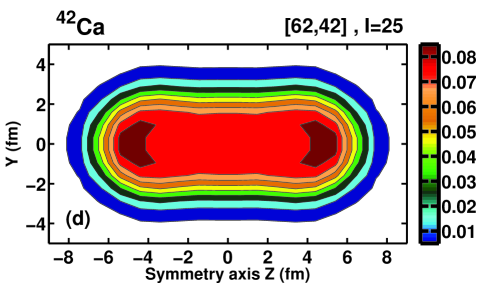
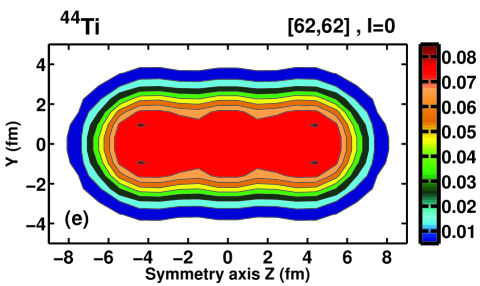
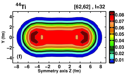
Figure 33: (Color online) The impact of rotation on the proton density distribution in selected configurations.

One of the main goals of the present paper is the search for possible candidates showing clusterization and molecular structures in the near-yrast region of the nuclei under study. Different single-particle states have different spatial density distributions which are dictated by their underlying nodal structure of their wavefunctions (see Fig. 9 in Ref. Afanasjev and Abusara (2010a)); the centers of the density distribution are found at the nodes and peaks of the oscillator eigenfunctions. The total density distribution is built as a sum of the single-particle density distributions of occupied single-particle states. Thus, for some specific occupations of the single-particle states at some deformations one may expect the effects in the density distributions which could be interpreted in terms of clusterization and molecular structures. Note that the structure of the wavefunctions of the single-particle orbitals is affected by rotation (see discussion in Sec. V of Ref. Afanasjev and Abusara (2010a)); this could lead to a modification of the single-particle density distributions (see Fig. 9 in Ref. Afanasjev and Abusara (2010a)). For some of the orbitals the effect of rotation on single-particle density distributions is quite substantial, while it has very little impact on the single-particle density distributions for others. This could lead either to a destruction or the emergence/enhancement of the clusterization and molecular structures with rotation.

Well known case of molecular structure in this mass region is the superdeformed configuration [2,2] in ³²S; according to Refs. Maruhn et al. (2006); Kimura and Horiuchi (2004) the wavefunction of this band contains significant admixture of the molecular ¹⁶O+¹⁶O structure. Indeed, the development of neck is seen in its density distribution (Fig. 29a). Similar neck exists also in the HD [21,21] configuration of ³²S (Fig. 29b) but the presence of density depressions at $z\sim\pm 2$ fm may suggest more complicated structure than the pair of two ¹⁶O. In addition, the neck is also present in the density distribution of the [31,21] configuration in ³⁴S but this configuration is characterized by an unusual density distribution with density depression in the highly elongated central region which is surrounded by the region of maximum density (Fig. 32). Note that the SD configurations, which have the structure of ¹⁶O+¹⁶O+two valence neutrons in molecular orbitals, have recently been predicted in the AMD+GCM calculations of Ref. Taniguchi (2014).

Present study reveals also a number of other interesting molecular structures which are discussed below. We were able to trace some of such configurations in an extended spin range starting from spin zero (or from very low spin), at which they are located at $20-30$ MeV excitation energy above the ground state, up to very high spin where they are either yrast or close to the yrast line. These are the [42,31] and [42,22] MD configurations in ³⁸Ar (Fig. 25), the [31,31] and [41,41] MD configurations in ³⁶Ar (Fig. 22), the [42,42] MD configuration in ⁴⁰Ca (Fig. 1), the [62,42] MD configuration in ⁴²Ca (Fig. 13), the [62,62] MD configurations in ⁴⁴Ti (Fig. 16) and [52,52] and [421,421] MD configurations in ⁴²Sc (Fig. 10). These examples allowed us to study the impact of rotation on clusterization.

The molecular structures become well pronounced in the [31,31] and [41,41] MD configurations of ³⁶Ar (Fig. 24c and d) which are characterized by well established neck. They are also seen in the [42,31] configuration of ³⁸Ar (Figs. 33a and b); note that in this case the rotation increases the separation of the fragments and makes the neck much more pronounced.

In ⁴⁰Ca, the density distribution of the MD [42,42] configuration at spin zero shows a triple-humped structure (top panel of Fig. 34). Similar configuration has been analyzed in Ref. Maruhn et al. (2006) and it was concluded that $\alpha$-cluster interpretation becomes quite fuzzy. Alternatively, one may consider this configuration as a ¹²C+¹⁶O+¹²C chain built of distorted ¹⁶O and ¹²C nuclei. The validity of such interpretation should be verified in future by comparison with the results of the cluster and/or antisymmetrized molecular (AMD) calculations similar to the ones presented in Ref. Maruhn et al. (2006). The comparison of the density distributions for this configurations at $I=0\hbar$ and $I=25\hbar$ (see Fig. 34) shows that the rotation hinders the tendency for clusterization. Indeed, the central hump becomes less pronounced and the depressions in the density distributions develop in central parts of the left and right segments at $I=25\hbar$ (bottom panel of Fig. 34).

Similar effects are also seen in the MD [42,22] configuration of ³⁸Ar (see Fig. 7 in the supplemental material (Ref. Sup ) which could be considered as the MD [42,42] configuration of ⁴⁰Ca with two proton holes in the $N=3$ orbitals. The addition of two neutrons to the MD [42,42] configuration of ⁴⁰Ca creates the MD [62,42] configuration in ⁴²Ca which has the features in the proton density distribution (see Figs. 33c and d) similar to the ones seen in Fig. 34.

These results show that in few configurations discussed above the rotation tries to suppress the features of the density distribution which could be attributed to the clusterization. However, the density modifications induced by rotation definitely depend on the nucleonic configuration. For example, the density distribution of the [62,62] configuration in ⁴⁸Cr is modified only modestly by rotation (see Figs. 2f and g in the supplemental material (Ref. Sup ). Note that this configuration does not show the features typical for clusterization. On the other hand, with increasing spin the separation of the fragments becomes larger and the neck becomes more pronounced in the [42,31] configuration of ³⁸Ar (Figs. 33a and b) and the [421,421] configuration of ⁴²Sc (Fig. 12c and d).

Another interesting case of possible clusterization is the [62,62] MD configuration in ⁴⁴Ti (Fig. 33e and f). Three fragments are clearly seen in the density distribution at $I=0\hbar$ indicating possible ¹⁶O+¹²C+¹⁶O chain of nuclei. Note that with rotation the central fragment dissolves but two outer segments became slightly more pronounced. It is interesting that similar three fragments structure survives in the [52,52] MD configuration up to very high spins in ⁴²Sc (Fig. 12b). This configuration could be considered as built from the [62,62] one in ⁴⁴Ti by creating proton and neutron holes in the $N=3$ orbital.

Very interesting case of molecular structures is seen on the example of the [421,421] MD configuration in ⁴²Sc (Figs. 12c and d and and Fig. 1a in the supplemental material (Ref. Sup ). This system could probably be described as a combination of two prolate deformed ²⁰Ne cores located in tip-to-tip arrangement with extra proton and neutron.

It is necessary to understand that suggested interpretations of molecular structures are based on the consideration of only density distributions. Their validity should be verified in future by the analysis of the wavefunctions of the underlying configurations (and their overlaps with mean field solutions) obtained in the cluster and/or antisymmetrized molecular dynamics calculations similar to the ones presented in Refs. Kimura and Horiuchi (2004); Maruhn et al. (2006).

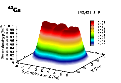
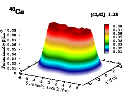
Figure 34: (Color online) Three-dimensional representation of the evolution or proton density distribution with spin in the [42,42] configuration of ⁴⁰Ca.

VIII Rotational properties of extremely deformed configurations

Most important physical observables characterizing the SD, HD and MD structures are kinematic ($J^{(1)}$) and dynamic ($J^{(2)}$) moments of inertia and transition quadrupole moments $Q_{t}$. The latter provides a direct information on the deformation of the charge distributions and that was a reason why the calculated $Q_{t}$ values were presented earlier. It is however necessary to recognize that previous history of the experimental investigation of the SD bands clearly shows that the $Q_{t}$ quantity is measured in dedicated experiment and thus it is available only for small fraction of the SD bands.

Thus it is expected that in future experiments it will be easier to obtain the information on rotational properties of the bands which are described in terms of kinematic and dynamic moments of inertia using the following expressions

$$J^{(1)}(\Omega_{x}) = J\left(\frac{dE}{dJ}\right)^{-1}=\frac{J}{\Omega_{x}},$$ (3)

$$J^{(2)}(\Omega_{x}) = J\left(\frac{d^{2}E}{dJ^{2}}\right)^{-1}=\frac{dJ}{d\Omega_{x}},$$ (4)

where

$$\Omega_{x}=\frac{dE}{dJ},$$ (5)

defines the rotational frequency and $E$ and $J$ are total energy and the expectation value of total angular momentum on the axis of rotation, respectively. Their experimental counterparts are extracted from the observed energies of the $\gamma$-transitions within a band according to the prescription given in Sec. 4.1 of Ref. Afanasjev et al. (1999a). Note that the kinematic moment of inertia depends on the absolute values of spins, while only the differences $\Delta I=2$ enter the definition of dynamic moment of inertia.

The SD bands observed in the $A\sim 40$ mass region are exception from the general rule that the SD bands are very seldom linked to the low-spin level scheme. Thus, contrary to absolute majority of the SD bands in nuclear chart their spins are known; it is quite likely that some SD bands which will be observed in this mass region in future will follow this pattern. On the contrary, it is expected that the spins of the HD and MD bands will be difficult to define in future experiments. For such bands, only dynamic moment of inertia will be available for comparison with the results of calculations.

The kinematic and dynamic moments of inertia of the (typically lowest in energy) SD, HD and MD bands are presented in Fig. 35 for each nucleus under study. For majority of the SD and HD bands one observes that the following condition $J^{(1)}\geq J^{(2)}$ is satisfied at medium and high frequencies. As discussed in Ref. Afanasjev et al. (1999a) this condition is valid for the rotational bands in unpaired regime. This condition is not valid in the region of unpaired band crossing with weak interaction where $J^{(2)}$ grows rapidly with increasing rotational frequency. This takes place at the highest calculated frequencies in the [2,2] SD configuration of ³²S (Fig. 35a), [4,4] SD configuration in ⁴⁰Ca (Fig. 35e), and [62,62] HD configuration in ⁴⁸Cr (Fig. 35k). Note also that such situation is seen at medium spin in the [31,21] HD configuration of ³⁴S (Fig. 35b) and the [51,4] SD configuration of ⁴⁴Ca (Fig. 35g).

The moments of inertia of the MD bands show three different patterns of behavior. Some of the MD bands undergo a centrifugal stretching that result in an increase of the transition quadrupole moments $Q_{t}$ with increasing rotational frequency. This process also reveals itself in the moments of inertia: the kinematic moments of inertia are either nearly constant or slightly increase with increasing rotational frequency, whereas the dynamic moments of inertia show two patterns of behavior. In one of them the dynamic moment of inertia is almost the same as kinematic one at low to medium rotational frequencies but then $J^{(2)}$ becomes bigger than $J^{(1)}$ and the difference between them gradually increases with frequency. These are the MD configurations shown in Figs. 35e, f, g and i. The pattern of the behavior of the [421,421] MD configuration in ⁴²Sc is very different (Fig. 35h); both moments increase with increasing rotational frequency but $J^{(2)}\geq J^{(1)}$ at all calculated frequencies. Note that this configuration has most elongated density distribution among studied in the present paper with clear indication of molecular structure (see Sec. III.) The rotational properties of above discussed MD bands are very similar to the HD ones in the $Z=40-58$ mass region investigated in Ref. Afanasjev and Abusara (2008); Abusara and Afanasjev (2009). On the other hand, the [31,31] MD configuration in ³⁶Ar (Fig. 35c) and [42,31] MD configuration in ³⁸Ar (Fig. 35d) show the relative properties of the two moments similar to the ones seen in the majority of the SD and HD bands shown in Fig. 35.

The examples shown in Fig. 35 clearly indicate strong dependence of the calculated $J^{(1)}$ and $J^{(2)}$ values on the nucleonic configuration and frequency. In most of the cases, at medium and high rotational frequencies there is a correlation between the moments of inertia and deformation so that the moments of inertia increase with increasing deformation. However, there are exceptions from this observation. For example, the dynamic moments of inertia of the [4,4] SD and [41,41] HD configurations in ⁴²Sc are quite similar (see Fig. 35h) despite substantial difference in the transition quadrupole moments (see Fig. 11a). Even more striking example is the similarity of dynamic moments of inertia of the [3,3] SD and [31,31] MD configurations in ³⁶Ar (Fig. 35c). Such similarities are also seen for the kinematic moments of inertia as illustrated by the case of the [52,52] SD and [62,62] HD bands in ⁴⁸Cr (Fig. 35k). Thus, the decision on the nature of the band (SD, HD or MD) observed in experiment cannot be based solely on the measured values of dynamic or kinematic moments of inertia; only the measurement of the transition quadrupole moment can reveal the true nature of the band.

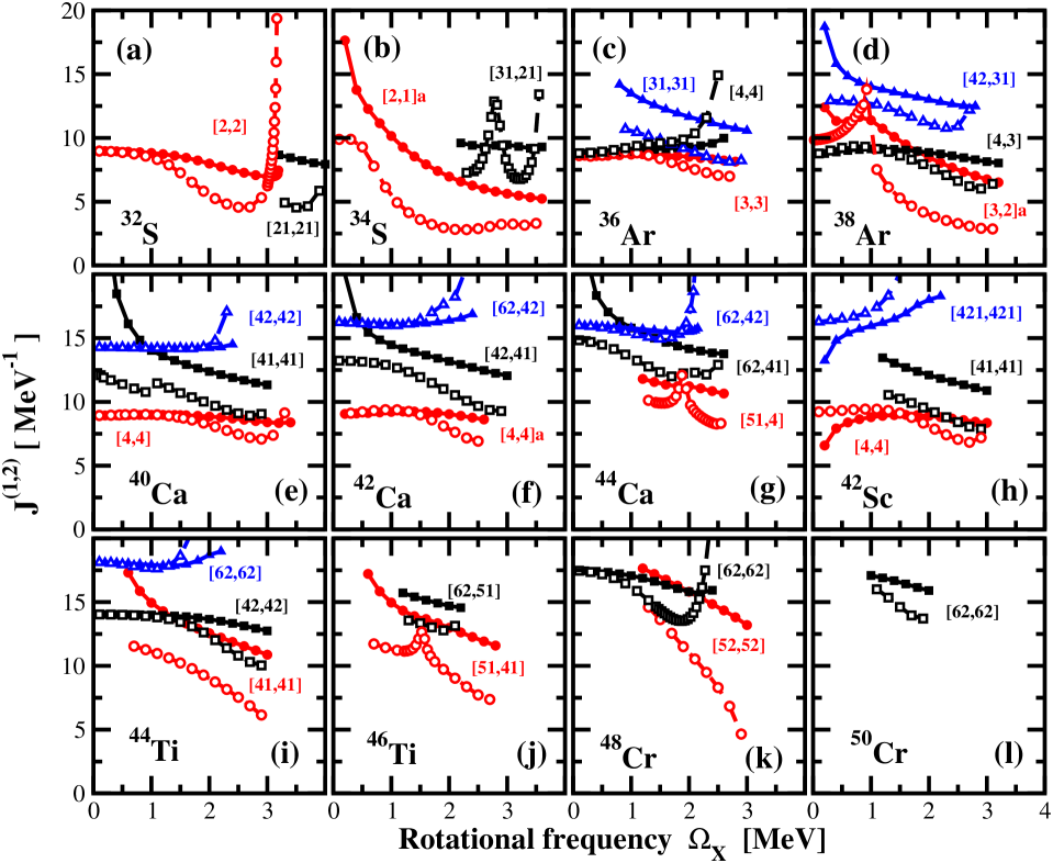
Figure 35: (Color online) Kinematic ($J^{(1)}$) and dynamic ($J^{(2)}$) moments of inertia of typical SD, HD and MD configurations in indicated nuclei. The calculated $J^{(1)}$ and $J^{(2)}$ values are shown by solid and open symbols, respectively. Red circles, black squares and blue triangles are used for the SD, HD and MD configurations, respectively.

IX Conclusions

A systematic search for extremely deformed structures in the $N\sim Z$ $A\sim 40$ nuclei has been performed for the first time in the framework of covariant density functional theory. The aim of this study was to define at which spins such structures become yrast, their properties and to find the configurations showing the fingerprints of clusterization and molecular structures. The main results can be summarized as follows.

• Present investigation shows that extremely deformed structures inevitably become yrast with increasing spin in the nuclei under study. This is because normal and highly-deformed configurations forming the yrast line at low and medium spins have limited angular momentum content. The key question is at which spin the transition from terminating to extremely deformed configurations takes place. This is basically defined by the maximum spin which could be built in terminating configurations with limited number of particle-hole excitations across the respective spherical shell gaps. This spin is quite limited for particle-hole excitations across the proton $Z=20$ and neutron $N=20$ spherical shell gaps. As a result, the nuclei most favored for the observation of extremely deformed structures are located in the vicinity of ³⁶Ar and ⁴⁰Ca. For example, present calculations suggest that in ³⁶Ar the increase of spin above measured $I=16\hbar$ state is only possible by the population of the hyperdeformed band. On the contrary, the configurations built on particle-hole excitations across the spherical $N=28$ and $N=28$ gaps, which bring substantial amount of angular momentum, dominate the yrast line at medium spin (up to $I\sim 30\hbar$) in the Cr nuclei. As a result, only at higher spins extremely deformed configurations become yrast.

• Similar to previous studies in the medium mass nuclei Afanasjev and Abusara (2008); Abusara and Afanasjev (2009), present calculations indicate that the $N=Z$ nuclei are better candidates for the observation of extremely deformed structures as compared with the nuclei which have an excess of neutrons over protons since the transition to extremely deformed structures takes place at lower spins.

• The above discussed consideration of the most favored candidates for experimental observation of extremely deformed structures is based on the spins at which they become yrast in model calculations. However, it is expected that experimental observations will also depend on employed combination(s) of the target(s) and projectile(s) and respective cross-sections of the reactions. Taking this factor and related uncertainties into account the $N=Z$ and $N=Z+2$ S, Ar, Ca, and Ti isotopes should be considered as good candidates for experimental observation of extremely deformed structures. On the other hand, the experimental observation of such structures in the ^48,50Cr isotopes is clearly disfavored by the present analysis as compared with above mentioned $N=Z$ and $N=Z+2$ isotopes.

• The underlying single-particle structure of nucleonic configurations with specific nodal structure of the single-particle density distribution leads to a clusterization in the form of molecular structures. The calculations suggest that in some nuclei such structures are either yrast or close to yrast at high spin. Thus, their observation with new generation of $\gamma$-tracking detectors such as GRETA and AGATA may be possible in near future. The calculations with cluster or/and antisymmetrized molecular dynamics models are definitely needed in order to establish the weights of those clusters in the structure of total wavefunction.

• The impact of rotation on the density distribution and clusterization (molecular nature) depends sensitively on nucleonic configuration. The density distributions of some configurations are only weakly affected by rotation. The features typical for clusterization, which are present at zero spin, are washed away by rotation in other configurations. On the other hand, the clusterization is enhanced by rotation in some specific configurations; with increasing spin the separation of the fragments becomes larger and the neck becomes more pronounced.

• There is a strong dependence of the calculated kinematic and dynamic moments of inertia on the configuration and frequency. In most of the cases the moments of inertia increase with increasing deformation at medium and high rotational frequencies. However, there are exceptions from this observation. As a result, the decision on the nature of the band (SD, HD or MD) observed in experiment cannot be based solely on the measured values of dynamic or kinematic moments of inertia; only the measurement of transition quadrupole moments will reveal the true nature of the band.

X Acknowledgements

This material is based upon work supported by the U.S. Department of Energy, Office of Science, Office of Nuclear Physics under Award Number DE-SC0013037.

References

- Kanada-En’yo and Kimura (2005) Y. Kanada-En’yo and M. Kimura, Phys. Rev. C 72, 064322 (2005).
- von Oertzen et al. (2006) W. von Oertzen, M. Freer, and Y. Kanada-En’yo, Phys. Rep. 432, 43 (2006).
- Maruhn et al. (2006) J. A. Maruhn, M. Kimura, S. Schramm, P.-G. Reinhard, H. Horiuchi, and A. Tohsaki, Phys. Rev. C 74, 044311 (2006).
- Taniguchi et al. (2007) Y. Taniguchi, M. Kimura, Y. Kanada-En’yo, and H. Horiuchi, Phys. Rev. C 76, 044317 (2007).
- Reinhard et al. (2011) P.-G. Reinhard, J. A. Maruhn, A. S. Umar, and V. E. Oberacker, Phys. Rev. C 83, 034312 (2011).
- Ebran et al. (2012) J.-P. Ebran, E. Khan, T. Nikšić, and D. Vretenar, Nature 487, 341 (2012).
- Taniguchi (2014) Y. Taniguchi, Phys. Rev. C 90, 054308 (2014).
- Zhao et al. (2015) P. W. Zhao, N. Itagaki, and J. Meng, Phys. Rev. Lett. 115, 022501 (2015).
- Iwata et al. (2015) Y. Iwata, T. Ichikawa, N. Itagaki, J. A. Maruhn, and T. Otsuka, Phys. Rev. C 92, 011303 (2015).
- Jenkins (2016) D. Jenkins, J. Phys. G 43, 024003 (2016).
- Kimura and Horiuchi (2004) M. Kimura and H. Horiuchi, Phys. Rev. C 69, 051304 (2004).
- Ebran et al. (2014) J.-P. Ebran, E. Khan, T. Nikšić, and D. Vretenar, Phys. Rev. C 90, 054329 (2014).
- Egido and Robledo (2004) J. L. Egido and L. M. Robledo, Nucl. Phys. A 738, 31 (2004).
- Yao et al. (2014) J. M. Yao, N. Itagaki, and J. Meng, Phys. Rev. C 90, 054307 (2014).
- Arumugam et al. (2005) P. Arumugam, B. K. Sharma, S. K. Patra, and R. K. Gupta, Phys. Rev. C 71, 064308 (2005).
- Ichikawa et al. (2011) T. Ichikawa, J. A. Maruhn, N. Itagaki, and S. Ohkubo, Phys. Rev. Lett. 107, 112501 (2011).
- Morinaga (1956) H. Morinaga, Phys. Rev. 101, 254 (1956).
- Hoyle (1954) F. Hoyle, Astr. J. Suppl. 1, 121 (1954).
- Afanasjev and Abusara (2008) A. V. Afanasjev and H. Abusara, Phys. Rev. C 78, 014315 (2008).
- Afanasjev et al. (1999a) A. V. Afanasjev, D. B. Fossan, G. J. Lane, and I. Ragnarsson, Phys. Rep. 322, 1 (1999a).
- Dudek et al. (2004) J. Dudek, K. Pomorski, N. Schunck, and N. Dubray, Eur. Phys. J A20, 15 (2004).
- Ideguchi et al. (2001) E. Ideguchi, D. G. Sarantites, W. Reviol, A. V. Afanasjev, M. Devlin, C. Baktash, R. V. F. Janssens, D. Rudolph, A. Axelsson, M. P. Carpenter, A. Galindo-Uribarri, D. R. LaFosse, T. Lauritsen, F. Lerma, C. J. Lister, P. Reiter, D. Seweryniak, M. Weiszflog, and J. N. Wilson, Phys. Rev. Lett. 87, 222501 (2001).
- Zhang and Rae (1993) J. Zhang and W. Rae, Nucl. Phys. A 564, 252 (1993).
- Chiara et al. (2003) C. J. Chiara, E. Ideguchi, M. Devlin, D. R. LaFosse, F. Lerma, W. Reviol, S. K. Ryu, D. G. Sarantites, C. Baktash, A. Galindo-Uribarri, M. P. Carpenter, R. V. F. Janssens, T. Lauritsen, C. J. Lister, P. Reiter, D. Seweryniak, P. Fallon, A. Görgen, A. O. Macchiavelli, and D. Rudolph, Phys. Rev. C 67, 041303 (2003).
- Svensson et al. (2000) C. E. Svensson, A. O. Macchiavelli, A. Juodagalvis, A. Poves, I. Ragnarsson, S. Åberg, D. E. Appelbe, R. A. E. Austin, C. Baktash, G. C. Ball, M. P. Carpenter, E. Caurier, R. M. Clark, M. Cromaz, M. A. Deleplanque, R. M. Diamond, P. Fallon, M. Furlotti, A. Galindo-Uribarri, R. V. F. Janssens, G. J. Lane, I. Y. Lee, M. Lipoglavsek, F. Nowacki, S. D. Paul, D. C. Radford, D. G. Sarantites, D. Seweryniak, F. S. Stephens, V. Tomov, K. Vetter, D. Ward, and C. H. Yu, Phys. Rev. Lett. 85, 2693 (2000).
- Svensson et al. (2001) C. E. Svensson, A. O. Macchiavelli, A. Juodagalvis, A. Poves, I. Ragnarsson, S. Åberg, D. E. Appelbe, R. A. E. Austin, G. C. Ball, M. P. Carpenter, E. Caurier, R. M. Clark, M. Cromaz, M. A. Deleplanque, R. M. Diamond, P. Fallon, R. V. F. Janssens, G. J. Lane, I. Y. Lee, F. Nowacki, D. G. Sarantites, F. S. Stephens, K. Vetter, and D. Ward, Phys. Rev. C 63, 061301 (2001).
- Bisoi et al. (2013) A. Bisoi, M. S. Sarkar, S. Sarkar, S. Ray, M. R. Basu, D. Kanjilal, S. Nag, K. Selvakumar, A. Goswami, N. Madhavan, S. Muralithar, and R. K. Bhowmik, Phys. Rev. C 88, 034303 (2013).
- Ideguchi et al. (2010) E. Ideguchi, S. Ota, T. Morikawa, M. Oshima, M. Koizumi, Y. Toh, A. Kimura, H. Harada, K. Furutaka, S. Nakamura, F. Kitatani, Y. Hatsukawa, T. Shizuma, M. Sugawara, H. Miyatake, Y. X. Watanabe, Y. Hirayama, and M. Oi, Phys. Lett. B 686, 18 (2010).
- Jenkins et al. (2012) D. G. Jenkins, C. J. Lister, M. P. Carpenter, P. Chowdury, N. J. Hammond, R. V. F. Janssens, T. L. Khoo, T. Lauritsen, D. Seweryniak, T. Davinson, P. J. Woods, A. Jokinen, H. Penttila, F. Haas, and S. Courtin, Phys. Rev. C 86, 064308 (2012).
- Di Nitto et al. (2016) A. Di Nitto, E. Vardaci, A. Brondi, G. La Rana, M. Cinausero, N. Gelli, R. Moro, P. N. Nadtochy, G. Prete, and A. Vanzanella, Phys. Rev. C 93, 044602 (2016).
- Papka et al. (2003) P. Papka, C. Beck, F. Haas, V. Raugh, M. Rousseau, P. Bednarczyk, S. Courtin, O. Dorvaux, K. Eddahbi, J. Robin, and A. S. i Zafra, Acta Phys. Pol. B34, 2343 (2003).
- Chiara et al. (2007) C. J. Chiara, M. Devlin, E. Ideguchi, D. R. LaFosse, F. Lerma, W. Reviol, S. K. Ryu, D. G. Sarantites, O. L. Pechenaya, C. Baktash, A. Galindo-Uribarri, M. P. Carpenter, R. V. F. Janssens, T. Lauritsen, C. J. Lister, P. Reiter, D. Seweryniak, P. Fallon, A. Görgen, A. O. Macchiavelli, D. Rudolph, G. Stoitcheva, and W. E. Ormand, Phys. Rev. C 75, 054305 (2007).
- Bisoi et al. (2014a) A. Bisoi, M. S. Sarkar, S. Sarkar, S. Ray, D. Pramanik, R. Kshetri, S. Nag, K. Selvakumar, P. Singh, A. Goswami, S. Saha, J. Sethi, T. Trivedi, B. S. Naidu, R. Donthi, V. Nanal, and R. Palit, Phys. Rev. C 89, 024303 (2014a).
- Aydin et al. (2014) S. Aydin, M. Ionescu-Bujor, F. Recchia, S. M. Lenzi, M. Bouhelal, D. Bazzacco, P. G. Bizzeti, A. M. Bizzeti-Sona, G. de Angelis, I. Deloncle, E. Farnea, A. Gadea, A. Gottardo, F. Haas, T. Huyuk, H. Laftchiev, S. Lunardi, D. Mengoni, R. Menegazzo, C. Michelagnoli, D. R. Napoli, A. Poves, E. Sahin, P. P. Singh, D. Tonev, C. A. Ur, and J. J. Valiente-Dobón, Phys. Rev. C 89, 014310 (2014).
- Bisoi et al. (2014b) A. Bisoi, M. S. Sarkar, S. Sarkar, S. Ray, D. Pramanik, R. Kshetri, S. Nag, K. Selvakumar, P. Singh, A. Goswami, S. Saha, J. Sethi, T. Trivedi, B. S. Naidu, R. Donthi, V. Nanal, and R. Palit, Phys. Rev. C 90, 024328 (2014b).
- Bender et al. (2003) M. Bender, H. Flocard, and P. H. Heenen, Phys. Rev. C 68, 044321 (2003).
- Yamagami and Matsuyanagi (2000) M. Yamagami and K. Matsuyanagi, Nucl. Phys. A 672, 123 (2000).
- Inakura et al. (2002) T. Inakura, S. Mizutori, M. Yamagami, and K. Matsuyanagi, Nucl. Phys. A 710, 261 (2002).
- Molique et al. (2000) H. Molique, J. Dobaczewski, and J. Dudek, Phys. Rev. C 61, 044304 (2000).
- Rodríguez-Guzmán et al. (2000) R. R. Rodríguez-Guzmán, J. L. Egido, and L. M. Robledo, Phys. Rev. C 62, 054308 (2000).
- Afanasjev et al. (2000a) A. V. Afanasjev, P. Ring, and I. Ragnarsson, Proc. Int. Workshop PINGST2000 ”Selected topics on nuclei”, 2000, Lund, Sweden, Eds. D. Rudolph and M. Hellström , 183 (2000a).
- Taniguchi et al. (2010) Y. Taniguchi, Y. Kanada-En’yo, M. Kimura, K. Ikeda, H. Horiuchi, and E. Ideguchi, Phys. Rev. C 82, 011302 (2010).
- Vretenar et al. (2005) D. Vretenar, A. V. Afanasjev, G. A. Lalazissis, and P. Ring, Phys. Rep. 409, 101 (2005).
- Afanasjev (2008) A. V. Afanasjev, Phys. Rev. C 78, 054303 (2008).
- Flocard et al. (1982) H. Flocard, P. H. Heenen, S. J. Krieger, and M. S. Weiss, Nucl. Phys. A 391, 285 (1982).
- Koepf and Ring (1989) W. Koepf and P. Ring, Nucl. Phys. A 493, 61 (1989).
- Afanasjev and Abusara (2010a) A. V. Afanasjev and H. Abusara, Phys. Rev. C 82, 034329 (2010a).
- Caurier et al. (1995) E. Caurier, J. L. Egido, G. Martínez-Pinedo, A. Poves, J. Retamosa, L. M. Robledo, and A. P. Zuker, Phys. Rev. Lett. 75, 2466 (1995).
- Serot and Walecka (1986) B. D. Serot and J. D. Walecka, Adv. Nucl. Phys. 16, 1 (1986).
- Reinhard (1989) P.-G. Reinhard, Rep. Prog. Phys. 52, 439 (1989).
- König and Ring (1993) J. König and P. Ring, Phys. Rev. Lett. 71, 3079 (1993).
- Afanasjev et al. (1996) A. V. Afanasjev, J. König, and P. Ring, Nucl. Phys. A 608, 107 (1996).
- Afanasjev and Frauendorf (2005) A. V. Afanasjev and S. Frauendorf, Phys. Rev. C 71, 064318 (2005).
- Afanasjev et al. (1999b) A. V. Afanasjev, I. Ragnarsson, and P. Ring, Phys. Rev. C 59, 3166 (1999b).
- Afanasjev et al. (2012) A. V. Afanasjev, Y. Shi, and W. Nazarewicz, Phys. Rev. C 86, 031304(R) (2012).
- Afanasjev (2016) A. V. Afanasjev, “Relativistic Density Functional for Nuclear Structure”, (World Scientific Publishing Co), Edited by Jie Meng, Int. Rev. Nucl. Phys. 10, 305 (2016).
- Afanasjev and Abdurazakov (2013) A. V. Afanasjev and O. Abdurazakov, Phys. Rev. C 88, 014320 (2013).
- Afanasjev and Abusara (2010b) A. V. Afanasjev and H. Abusara, Phys. Rev. C 81, 014309 (2010b).
- Afanasjev and Ring (2000) A. V. Afanasjev and P. Ring, Phys. Rev. C 62, 031302(R) (2000).
- Petermann et al. (2012) I. Petermann, K. Langanke, G. Martinez-Pinedo, I. V. Panov, P.-G. Reinhard, and F.-K. Thielemann, Eur. Phys. J. A 48, 122 (2012).
- Ring and Schuck (1980) P. Ring and P. Schuck, The Nuclear Many-Body Problem (Springer-Verlag, Berlin) (1980).
- de Voigt et al. (1983) M. J. A. de Voigt, J. Dudek, and Z. Szymański, Rev. Mod. Phys. 55, 949 (1983).
- Shimizu et al. (1989) Y. R. Shimizu, J. D. Garrett, R. A. Broglia, M. Gallardo, and E. Vigezzi, Rev. Mod. Phys. 61, 131 (1989).
- Afanasjev et al. (2000b) A. V. Afanasjev, P. Ring, and J. König, Nucl. Phys. A676, 196 (2000b).
- Dobaczewski et al. (2015) J. Dobaczewski, A. V. Afanasjev, M. Bender, L. M. Robledo, and Y. Shi, Nucl. Phys. A 944, 388 (2015).
- Lalazissis et al. (2009) G. A. Lalazissis, S. Karatzikos, R. Fossion, D. P. Arteaga, A. V. Afanasjev, and P. Ring, Phys. Lett. B671, 36 (2009).
- Agbemava et al. (2014) S. E. Agbemava, A. V. Afanasjev, D. Ray, and P. Ring, Phys. Rev. C 89, 054320 (2014).
- Afanasjev and Shawaqfeh (2011) A. V. Afanasjev and S. Shawaqfeh, Phys. Lett. B 706, 177 (2011).
- Abusara et al. (2010) H. Abusara, A. V. Afanasjev, and P. Ring, Phys. Rev. C 82, 044303 (2010).
- Afanasjev et al. (2003) A. V. Afanasjev, T. L. Khoo, S. Frauendorf, G. A. Lalazissis, and I. Ahmad, Phys. Rev. C 67, 024309 (2003).
- Hilaire and Girod (2007) S. Hilaire and M. Girod, Eur. Phys. J. 33, 237 (2007).
- Samyn et al. (2005) M. Samyn, S. Goriely, and J. M. Pearson, Phys. Rev. C 72, 044316 (2005).
- (73) W. Nazarewicz and I. Ragnarsson, Nuclear deformations in Handbook on nuclear properties, Eds. D. N. Poenaru and W. Greiner (Claredon Press, Oxford, 1996) , 80.
- Caurier et al. (2007) E. Caurier, J. Menéndez, F. Nowacki, and A. Poves, Phys. Rev. C 75, 054317 (2007).
- Abusara and Afanasjev (2009) H. Abusara and A. V. Afanasjev, Phys. Rev. C 79, 024317 (2009).
- Andreoiu et al. (2007) C. Andreoiu, C. E. Svensson, A. V. Afanasjev, R. A. E. Austin, M. P. Carpenter, D. Dashdorj, P. Finlay, S. J. Freeman, P. E. Garrett, J. Greene, G. F. Grinyer, A. Görgen, B. Hyland, D. Jenkins, F. Johnston-Theasby, P. Joshi, A. O. Machiavelli, F. Moore, G. Mukherjee, A. A. Phillips, W. Reviol, D. G. Sarantites, M. A. Schumaker, D. Seweryniak, M. B. Smith, J. J. Valiente-Dobón, and R. Wadsworth, Phys. Rev. C 75, 041301 (2007).
- O’Leary et al. (2003) C. D. O’Leary, C. E. Svensson, S. G. Frauendorf, A. V. Afanasjev, D. E. Appelbe, R. A. E. Austin, G. C. Ball, J. A. Cameron, R. M. Clark, M. Cromaz, P. Fallon, D. F. Hodgson, N. S. Kelsall, A. O. Macchiavelli, I. Ragnarsson, D. Sarantites, J. C. Waddington, and R. Wadsworth, Phys. Rev. C 67, 021301(R) (2003).
- Brandolini et al. (1998) F. Brandolini, S. Lenzi, D. Napoli, R. Ribas, H. Somacal, C. Ur, D. Bazzacco, J. Cameron, G. de Angelis, M. D. Poli, C. Fahlander, A. Gadea, S. Lunardi, G. Martinez-Pinedo, N. Medina, C. R. Alvarez, J. Sanchez-Solano, and C. Svensson, Nucl. Phys. A 642, 387 (1998).
- (79) See Supplemental Material at [URL will be inserted by publisher] for the results of the calculations not included into main body of the manuscript .
- Caurier et al. (2005) E. Caurier, F. Nowacki, and A. Poves, Phys. Rev. Lett. 95, 042502 (2005).
- Sheline et al. (1972) R. Sheline, I. Ragnarsson, and S. Nilsson, Phys. Lett. B 41, 115 (1972).
- Leander and Larsson (1975) G. Leander and S. Larsson, Nucl. Phys. A 239, 93 (1975).
- Tanaka et al. (2001) T. Tanaka, R. G. Nazmitdinov, and K. Iwasawa, Phys. Rev. C 63, 034309 (2001).