Poisson-Boltzmann study of the effective electrostatic interaction between colloids at an electrolyte interface

Abstract

The effective electrostatic interaction between a pair of colloids, both of them located close to each other at an electrolyte interface, is studied by employing the full, nonlinear Poisson-Boltzmann (PB) theory within classical density functional theory. Using a simplified yet appropriate model, all contributions to the effective interaction are obtained exactly, albeit numerically. The comparison between our results and those obtained within linearized PB theory reveals that the latter overestimates these contributions significantly at short inter-particle separations. Whereas the surface contributions to the linear and the nonlinear PB results differ only quantitatively, the line contributions show qualitative differences at short separations. Moreover, a dependence of the line contribution on the solvation properties of the two adjacent fluids is found, which is absent within the linear theory. Our results are expected to enrich the understanding of effective interfacial interactions between colloids.

I Introduction

More than a century ago, Ramsden discovered that suspended colloidal particles show a strong affinity for fluid interfaces compared to the bulk Ram03 . This is due to a particle induced reduction of the interfacial area between the two fluids. Typically, the resulting decrease in the interfacial free energy is much larger than the thermal energy. Thus the attachment of the colloids to the interface is almost irreversible and the trapped particles form an effectively two-dimensional system. These colloidal monolayers are important for a wide range of industrial and biological proccesses. For example, emulsions, including many food emulsions, are stabilized by the adsorption of colloidal particles at liquid-liquid interfaces Dic89 ; Tam94 ; encapsulation and delivery of drugs or nutrients can be achieved through colloidosomes Din02 . Froth flotation, which involves the separation of hydrophilic from hydrophobic particles by attaching the latter to air bubbles in a suspension, plays a key role in mineral processing, water purification, oil recovery, bacteria separation, and for recycling of plastics Bin06 . Since the particles are confined only in the vertical direction but are free to move along the interfacial plane, the stability of such monolayer structures is, to a large extent, determined by the effective inter-particle interaction and therefore a proper understanding of this lateral interaction is highly desired.

The effective interaction between particles at an interface is quite different from that present in the bulk. All types of interactions, such as electrostatic, magnetic, or van der Waals, which are present in the bulk, are also present at the interface, albeit in a different form. On top of that, particles interact via deformations of the fluid interface, which can be generated by gravity, electric stress gradients, or magnetic fields Nik02 ; Oet05 ; For04 ; Oet08 . Here, however, we are not concerned with these interface-mediated capillary or elastic interactions, but we shall focus only on the electrostatically induced effective interaction between the particles. The evolution of the studies concerned with the electrostatic interaction in this context dates back to 1980, when Pieranski reported the two-dimensional crystallization of polystyrene particles at an air-water interface and attributed it to a purely repulsive, long-ranged dipolar interaction originating from the asymmetric counterion distribution across the interface and acting through air Pie80 . Hurd confirmed these predictions Hur85 , based on analytical calculations within the framework of linearized PB theory and on the assumption that the particles are separated by distances large compared to their radii. Later studies reported a weakening of the effective interaction upon increasing the ionic strength of the corresponding polar medium which differs from Hurd’s prediction Ave00 ; Ave02 ; Hor05 ; Par08 . As a possible explanation this has been linked to the relatively small amount of residual charges present at the particle-oil Ave00 ; Ave02 ; Par08 or the particle-air Hor05 interface, but an unanimous picture is still lacking.

A major simplification used in almost all studies mentioned above as well as in related studies consists of considering large inter-particle separations for which both the superposition approximation and the linearization of the PB equation are taken to be valid. The associated dipolar interaction is also a signature of this key simplification. But for short inter-particle distances Too16 , which is relevant for dense systems or self-organization processes, none of them are actually applicable. In a recent publication Maj14 , we have discussed the drawbacks of the superposition assumption not only at short inter-particle distances but also at large distances. The assumption concerning the linearization of the PB equation, which leads to the well known Debye-Hückel (DH) equation, requires the electrostatic energy of a single charge in solution to be much smaller than the thermal energy. While this might hold true at distances far from the particle, at short distances this is violated for most experimental setups. For highly charged colloids, which are also quite common, the situation becomes worse, even at relatively large distances. Moreover, nonlinear charge renormalization effects are known to alter the strength of the effective interaction potential significantly Fry07 . Hence, appropriate insight into the effective interaction between a pair of particles, especially at small separations, remains elusive without including nonlinearity. This formulates the goal of the present study.

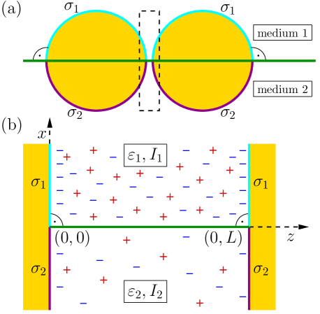
Figure 1: (a) Schematic illustration of two identical spherical particles each of which is partitioned equally between the two fluid phases separated by a flat interface (horizontal green line). The particles are close to each other with a contact angle of $90^{\circ}$. (b) Magnified view of the boxed region in (a). Due to the small distance between them, the particles are treated as parallel, planar walls at a distance $L$. The region between the walls is filled with two immiscible fluids with permittivities $\varepsilon_{1}$, $\varepsilon_{2}$ and ionic strengths $I_{1}$, $I_{2}$ respectively. The surface charge density on each wall is $\sigma_{1}$ ($\sigma_{2}$) at the contact with medium “1” (“2”). The system depicted here corresponds to the case in which medium “1” is the more polar phase and that the walls are positively charged on both sides of the horizontal fluid-fluid interface.

Even a mean-field description like the PB equation, which is adequate to describe interfacial structures above the atomic scale, poses already a significant challenge. Therefore, we numerically solve a simplified model by replacing the spherical particles with planar walls in the spirit of the Derjaguin approximation (see Fig. 1) Rus89 . This simplification is justified because we focus on short inter-particle separations only. The validity of such an assumption has been verified also for infinitely long cylinders at an oil-water interface Lyn92 . In addition, we consider the particles to float on a flat interface and that they are immersed in both fluid phases to the same extent. This corresponds to a liquid-particle contact angle of $90^{\circ}$ which is equal or close to what one observes in many experimental systems Ave03 ; Rei04 ; Mas10 . In fact, it is known that for high stability of particle-stabilized emulsions, the contact angle should not deviate strongly from $90^{\circ}$ Ave03 . In order to keep the present investigation general and in order to be consistent with previous experimental studies Ave00 ; Ave02 ; Par08 , we consider surface charges on both sides of the fluid-fluid-interface. The electrostatic problem for this model system is solved by employing the framework of density functional theory Eva79 and the resulting effective interaction energy is divided into two parts: a surface contribution, expressed per total surface area, and a line contribution per total length of the two three-phase contact lines formed by solid-liquid-liquid coexistence. A comparison of our results with those obtained within linear theory reveals both quantitative and qualitative differences concerning the effective line interaction energy (Figs. 2(e) and (f)), quantitative differences concerning the surface interaction energies (Figs. 2(a)–(d)), and a dependence of the line contribution on the solvation properties of the two adjacent fluids which is not captured by the linear theory (Fig. 4).

II Formalism

In a three-dimensional Cartesian coordinate system, the walls are considered to be placed at $z=0$ and $z=L$ and the two slabs ($x\gtrless 0$ with $0\leq z\leq L$) in between are filled with medium “1” $(x>0)$ and medium “2” $(x<0)$, respectively. The walls are chemically identical in nature but the surface charge density $\sigma(\mathbf{r})$ on each wall varies depending on the surrounding medium: $\sigma(\mathbf{r})=\sigma_{1}$ on the upper half planes ($x>0$) and $\sigma(\mathbf{r})=\sigma_{2}$ on the lower half planes ($x<0$). Since the layering of solvent molecules and ions takes place close to the walls and to the interface on the length scale of the bulk correlation length which, typically, is comparable to the molecular scale and which is much smaller than the length scale of interest here, the solvents in both media are taken to be structureless, homogeneous, linear dielectric fluids. Therefore, the permittivity $\varepsilon(\mathbf{r})$, which is the product of the relative permittivity $\varepsilon_{r}(\mathbf{r})$ and the permittivity $\varepsilon_{0}$ of vaccum, varies steplike at the interface between the fluids: $\varepsilon(\mathbf{r})=\varepsilon_{r,1}\varepsilon_{0}$ for $x>0$ and $\varepsilon(\mathbf{r})=\varepsilon_{r,2}\varepsilon_{0}$ for $x<0$. The solute is a simple binary salt with bulk ionic strength $I(\mathbf{r})=I_{1}$ ($I_{2}$) in medium “1”(“2”). Here, however, we consider the nonuniformity of the charge density $e\left(\varrho_{+}(\mathbf{r})-\varrho_{-}(\mathbf{r})\right)$, with $\varrho_{\pm}(\mathbf{r})$ denoting the number density of the $\pm$-ions, which varies on a length scale of the order of the Debye length which is usually much larger than the molecular length scale. We describe our system within the grand canonical ensemble with the ion reservoirs being provided by the bulk phases of both media. Considering the ions as point-like objects and ignoring ion-ion correlations, the grand canonical density functional corresponding to our system in the units of the thermal energy $k_{B}T=1/\beta$ is given by

$$\beta\Omega\left[\varrho_{\pm}\right]= \int\limits_{V}d^{3}r\Bigg{[}\sum\limits_{i=\pm}\varrho_{i}\left(\mathbf{r}\right)\Bigg{\{}\ln\left(\frac{\varrho_{i}\left(\mathbf{r}\right)}{\zeta_{i}}\right)-1$$

$$+\beta V_{i}\left(\mathbf{r}\right)\Bigg{\}}+\frac{\beta\mathbf{D}\left(\mathbf{r},\left[\varrho_{\pm}\right]\right)^{2}}{2\varepsilon\left(\mathbf{r}\right)}\Bigg{]},$$ (1)

where $\zeta_{\pm}$ are the fugacities of the two species of ions, $\mathbf{D}$ is the electric displacement field, and the integration volume $V$ is the space enclosed by the two walls. The first line of Eq. (1) represents the entropic ideal gas contribution of the ions. The first term in the second line describes the ion-solvent interaction expressed by an external potential $V_{\pm}(\mathbf{r})$ acting on the ions Bie12 . The last term corresponds to the ion-ion Coulomb interaction. First, one determines the equilibrium density profiles $\varrho_{\pm}^{\text{eq}}$, which minimize the grand potential in Eq. (1). Second, these equilibrium profiles are inserted into the grand potential functional in order to infer the equilibrium grand potential $\beta\Omega^{\text{eq}}(L)=\beta\Omega\left[\varrho_{\pm}^{\text{eq}}\right]$. In the course of this minimization process, one encounters the relation

$$\varrho_{\pm}^{\text{eq}}(\mathbf{r})=I(\mathbf{r})\exp\left\{\mp\beta e\left(\Phi\left(\mathbf{r},[\varrho_{\pm}^{\text{eq}}]\right)-\Phi_{b}(\mathbf{r})\right)\right\}$$ (2)

with the electrostatic potential $\Phi(\mathbf{r},[\varrho_{\pm}^{\text{eq}}])$ satisfying the nonlinear Poisson-Boltzmann equation

$$\nabla^{2}\left(\beta e\Phi\left(\mathbf{r}\right)\right) =\kappa(\mathbf{r})^{2}\sinh\left\{\beta e\left(\Phi\left(\mathbf{r}\right)-\Phi_{b}(\mathbf{r})\right)\right\}$$ (3)

everywhere except for $x=0$. We note that from here onwards for reasons of brevity the functional dependence of $\Phi$ on $\varrho_{\pm}^{\text{eq}}$ is not indicated explicitly. The associated boundary conditions are: (i) the electrostatic potential should remain finite for $x\rightarrow\pm\infty$, (ii) both the electrostatic potential and the normal component of the electric displacement field should be continuous at the fluid interface, i.e., $\Phi(x=0^{+})=\Phi(x=0^{-})$ and $\varepsilon_{r,1}\partial_{x}\Phi(x=0^{+})=\varepsilon_{r,2}\partial_{x}\Phi(x=0^{-})$, and (iii) in order to satisfy global charge neutrality, the normal component of the electric displacement field should match the surface charge densities at both walls, i.e., $\varepsilon(\mathbf{r})\partial_{z}\Phi(z=0)=\sigma(\mathbf{r})$ and $\varepsilon(\mathbf{r})\partial_{z}\Phi(z=L)=-\sigma(\mathbf{r})$. In Eq. (3), $\kappa(\mathbf{r})=\sqrt{8\pi\ell_{B}I(\mathbf{r})/\varepsilon_{r}(\mathbf{r})}$ is the inverse Debye screening length with the Bjerrum length $\ell_{B}=e^{2}/(4\pi\varepsilon_{0}k_{B}T)$, $e>0$ is the elementary charge, and $\Phi_{b}(\mathbf{r})$ represents the electrostatic potential in the bulk of the two media which is defined such that $\Phi_{b}(\mathbf{r})=0$ in medium “1” ($x>0$) and $\Phi_{b}(\mathbf{r})=\Phi_{D}$ in medium “2” ($x<0$). $\Phi_{D}$ originates from a difference in the solubilities of the ions in the two fluids and is called Donnan potential or Galvani potential difference between the two media Bag06 .

In order to numerically determine $\Phi(\mathbf{r})$, which solves Eq. (3) and fulfills the boundary conditions (i)–(iii), we use a Rayleigh-Ritz-like finite element method (fem) based on the minimization of the functional

$$\beta\Omega_{\text{fem}}\left[\Phi\right]= \int\limits_{V}d^{3}r\Bigg{[}2I(\mathbf{r})\cosh\left\{\beta e\left(\Phi(\mathbf{r})-\Phi_{b}(\mathbf{r})\right)\right\}$$

$$+\frac{\beta\varepsilon(\mathbf{r})}{2}\left\{\left(\partial_{x}\Phi(\mathbf{r})\right)^{2}+\left(\partial_{z}\Phi(\mathbf{r})\right)^{2}\right\}\Bigg{]}$$

$$-\int\limits_{\partial V}d^{2}r\sigma(\mathbf{r})\Phi(\mathbf{r}),$$ (4)

with $\partial V$ indicating the boundaries of the integration volume $V$. It can be shown that the minimum $\beta\Omega_{\text{fem}}^{\text{min}}(L)$ of Eq. (4) is related to the equilibrium grand potential $\beta\Omega^{\text{eq}}(L)$ by $\beta\Omega^{\text{eq}}(L)=-\beta\Omega_{\text{fem}}^{\text{min}}(L)$. In order to study the effect of nonlinearity, we expand the function $\cosh\left\{\beta e\left(\Phi(\mathbf{r})-\Phi_{b}(\mathbf{r})\right)\right\}$ in Eq. (4) in a Taylor series:

$$\beta\Omega_{\text{fem}}^{(n)}\left[\Phi\right]= \int\limits_{V}d^{3}r\Bigg{[}2I(\mathbf{r})\sum\limits_{k=0}^{n}\frac{\left\{\beta e\left(\Phi(\mathbf{r})-\Phi_{b}(\mathbf{r})\right)\right\}^{2k}}{(2k)!}$$

$$+\frac{\beta\varepsilon(\mathbf{r})}{2}\left\{\left(\partial_{x}\Phi(\mathbf{r})\right)^{2}+\left(\partial_{z}\Phi(\mathbf{r})\right)^{2}\right\}\Bigg{]}$$

$$-\int\limits_{\partial V}d^{2}r\sigma(\mathbf{r})\Phi(\mathbf{r}),$$ (5)

where $n$ describes the degree of the nonlinearity. For $n=1$, it reduces to the linearized PB problem and for $n\rightarrow\infty$ it corresponds to the full nonlinear problem (see Eq. (3)). First, we find the equilibrium profiles for the electrostatic potential $\Phi^{\text{eq}}$ which minimize the functional in Eq. (5) and then we insert it back into Eq. (5) in order to calculate the grand potential $\beta\Omega^{(n)\text{eq}}(L)=-\beta\Omega_{\text{fem}}^{(n)\text{min}}(L)$. The latter includes nine distinct contributions:

$$\Omega^{(n)\text{eq}}(L)= \sum\limits_{i\in\{1,2\}}\left[\Omega_{b,i}V_{i}+\left(\gamma_{i}+\omega_{\gamma,i}(L)\right)A_{i}\right]$$

$$+\gamma_{1,2}A_{1,2}+\left(\tau+\omega_{\tau}(L)\right)\ell,$$ (6)

where $\Omega_{b,i}$ is the bulk grand potential density (i.e., the negative osmotic pressure of the ions) in medium $i\in\{1,2\}$, $\gamma_{i}$ is the surface tension of a single wall in contact with medium $i$, $\omega_{\gamma,i}(L)$ is the surface interaction energy per total area of the two walls at distance $L$ in contact with medium $i$, $\gamma_{1,2}$ is the interfacial tension between the two fluid media, $\tau$ is the line tension of a single three-phase (solid-liquid-liquid) contact line, $\omega_{\tau}(L)$ is the line interaction energy per total line length of two three-phase contact lines at a distance $L$, $V_{i}$ is the volume of the slab between the two walls filled with medium $i$, $A_{i}$ is the total surface area of the two walls in contact with medium $i$, and $\ell$ is the total length of the two three-phase contact lines. In order to separate all these parts, we solve the following additional problems: (i) a single medium in the absence of any wall; the corresponding grand potential density is obtained by setting $\Phi(\mathbf{r})=\Phi_{b}(\mathbf{r})$ and $\sigma(\mathbf{r})=0$ in Eq. (5) which leads to $\Omega_{b,i}=-2I_{i}/\beta$, (ii) two fluid media forming an interface in the absence of any walls ($\sigma(\mathbf{r})=0$ in Eq. (5)), (iii) one homogeneously charged wall in contact with a single semi-infinite fluid medium, (iv) two homogeneously charged walls in contact with a single fluid medium in between, and (v) a single charged wall in contact with two immiscible semi-infinite fluids forming an interface along with a single three-phase contact line. Finally, a systematic subtraction of one interaction potential from another, which corresponds to one of the above mentioned problems, allows one to extract all individual contributions in Eq. (6). We note that, upon construction, all $L$-dependent contributions, i.e., $\omega_{\gamma,i}(L)$ and $\omega_{\tau}(L)$, vanish individually in the limit $L\rightarrow\infty$.

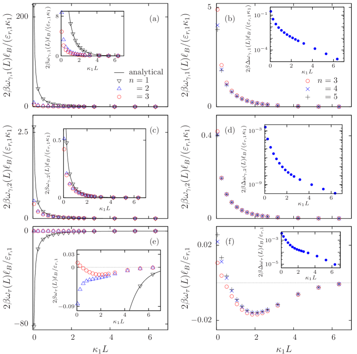
Figure 2: (a)–(d) Reduced surface interaction energies $\omega_{\gamma,i}(L)$ per total area of the two walls in contact with medium $i\in\{1,2\}$ and (e)–(f) reduced line interaction energy $\omega_{\tau}(L)$ per total length of the three-phase contact lines as functions of the wall separation $L$ (in units of the Debye screening length $1/\kappa_{1}$) for various degrees $n$ of nonlinearity (see Eq. (5)). For these plots the standard set of parameters ($\sigma=0.1$, $I=0.85$, $\varepsilon=62/72$, $b_{1}\approx 0.23$, $\beta e\Phi_{D}=1$, see the main text) corresponding to a water+lutidine mixture with KBr at $T=313\,\mathrm{K}$ is used. In the left panels, values for $1\leq n\leq 3$ are compared whereas in the right panels the values for $3\leq n\leq 5$ are compared. For $n=1$, our numerical results match perfectly with the corresponding analytical solutions (black solid line) taken from Ref. Maj14 . With increasing $n$, the magnitude of both $\omega_{\gamma,1}(L)$ and $\omega_{\gamma,2}(L)$ drop significantly at short separations, but the interactions remain repulsive everywhere. However, $\omega_{\tau}(L)$ shows qualitative changes upon increasing $n$. Whereas $\omega_{\tau}(L)$ is attractive at all separations both in the linear case ($n=1$) and for $n=2$, it is repulsive at short distances for $n\geq 3$. Due to the huge difference of magnitudes between the results obtained from the linear and the nonlinear theory, in the left panels magnified views are provided as insets. Since the differences $\Delta\omega_{\gamma,i}(L)=\omega_{\gamma,i}^{n=5}(L)-\omega_{\gamma,i}^{n=4}(L)$ with $i\in\{1,2\}$ and $\Delta\omega_{\tau}(L)=\omega_{\tau}^{n=5}(L)-\omega_{\tau}^{n=4}(L)$ are very small, the absolute values of these differences are displayed as insets in the right panels.

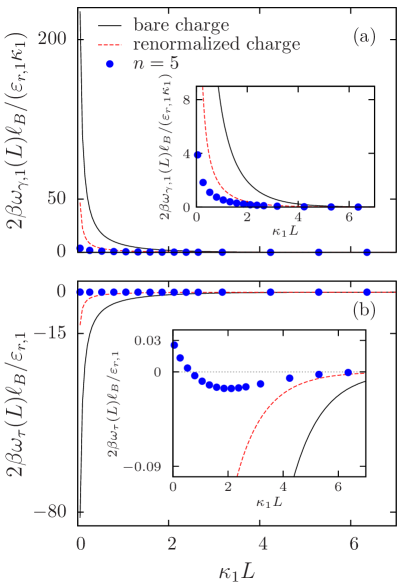
Figure 3: (a) Reduced surface interaction energy $\omega_{\gamma,1}(L)$ per total area of the two walls in contact with medium “1” and (b) reduced line interaction energy $\omega_{\tau}(L)$ per total length of the three-phase contact lines as functions of the scaled wall separation $\kappa_{1}L$ for three different cases: (i) The black solid lines correspond to the analytical solutions taken from Ref. Maj14 within linearized PB theory and with bare surface charge densities at the walls. (ii) The red dashed lines also correspond to the analytical solutions taken from Ref. Maj14 within linearized PB theory but with the renormalized surface charge density in medium “1”. (iii) The blue filled circles correspond to the numerical solutions within the nonlinear PB theory with the degree $n=5$ of nonlinearity. As in Fig. 2, the standard set of parameters is used for the plots (see the main text). The quantitative differences between linear and nonlinear results decrease upon using the renormalized surface charges. But still a significant mismatch remains to be present and the qualitative features obtained within the nonlinear theory remain unexplained by the linear theory even after taking into account the charge renormalization effect.

III Results and Discussion

III.1 $L$-dependent interactions

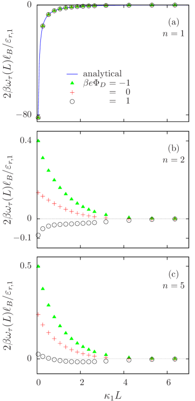
Figure 4: Line interaction energy $\omega_{\tau}(L)$ per total length of the three-phase contact lines expressed in units of $\varepsilon_{r,1}/(2\beta\ell_{B})$ as a function of the distance $L$ (in units of the Debye length $1/\kappa_{1}$) for three values of the dimensionless Donnan potential $\beta e\Phi_{D}$. (a) Within the linear theory ($n=1$), $\omega_{\tau}(L)$ is insensitive to varying $\beta e\Phi_{D}$ which is in accordance with the analytical results obtained within the linearized PB theory Maj14 . (b) However, for the degree $n=2$ of the nonlinearity, $\omega_{\tau}(L)$ varies upon changing $\beta e\Phi_{D}$. For $n\geq 4$ the line interaction curves $\omega_{\tau}(L)$ basically do not depend on $n$ anymore. (c) For $n=5$, $\omega_{\tau}(L)$ exhibits a minimum for $\beta e\Phi_{D}=1$ (which corresponds to its value within the standard set of parameters) but it is purely repulsive for $\beta e\Phi_{D}=-1$ and $0$ (even for $n=2$) whereas the linear theory predicts an attractive interaction.

In the following, we discuss all $L$-dependent contributions to the effective interaction between the walls as a function of the scaled wall separation $\kappa_{1}L$. Accordingly, both $\omega_{\gamma,i}(L)$ and $\omega_{\tau}(L)$ are rendered dimensionless by expressing them in units of $\varepsilon_{r,1}\kappa_{1}/(2\beta\ell_{B})$ and $\varepsilon_{r,1}/(2\beta\ell_{B})$, respectively. If done so, the dimensionless free parameters for our system turn out to be $\sigma=\sigma_{2}/\sigma_{1}$, $I=I_{2}/I_{1}$, $\varepsilon=\varepsilon_{r,2}/\varepsilon_{r,1}$, $\beta e\Phi_{D}$, and $b_{1}=\kappa_{1}\ell_{GC}^{(1)}$, where $\ell_{GC}^{(1)}=e\varepsilon_{r,1}/(2\pi\lvert\sigma_{1}\rvert\ell_{B})$ is the Gouy-Chapmann length for medium “1”. First, we discuss the results for a standard set of parameters ($\sigma_{\text{std}}=0.1$, $I_{\text{std}}=0.85$, $\varepsilon_{\text{std}}=62/72$, $b_{1}\approx 0.23$, $\beta e\Phi_{D}=1$) which corresponds to a typical experimental setup, e.g., a water-lutidine (2,6-dimethylpyridine) mixture with NaI salt ($1\,\mathrm{mM}$ in the aqueous phase) at temperature $T=313\,\mathrm{K}$ in contact with polystyrene walls exhibiting, in the aqueous phase, a surface charge density of $0.1\,e/\mathrm{nm^{2}}$ Ave02 ; Bie12 ; Gra93 ; Ine94 ; Ram58 ; Lid98 ; Gal92 . The resulting interaction energies are presented in Fig. 2. In each of the three plots, the symbols correspond to various values of the degree of nonlinearity $n$ in Eq. (5) and the solid lines correpond to the analytical solutions taken from Ref. Maj14 . Figures 2(a) and (b) show the reduced surface interaction energy $\omega_{\gamma,1}(L)$ between the walls in contact with medium “1” for a varying distance $L$ between the walls. While the interaction remains repulsive in all cases, obviously the linear theory overestimates the strength of the interaction at short distances. As expected, for $n=1$ (which corresponds to the linear theory), our numerical results match with the corresponding analytical results over the whole range of separations considered here. The most significant changes take place upon increasing the degree of nonlinearity $n$ from $n=1$ (linear theory) to $n=2$, whereas for $n\geq 4$ basically no changes occur upon increasing $n$ further. The surface interaction $\omega_{\gamma,1}(L)$ within the linear theory differs by orders of magnitude from the one within the nonlinear theory. For example, $\omega_{\gamma,1}(\kappa_{1}L=0.05)$ for $n=1$ is larger compared to that obtained for $n=5$ by almost a factor of $60$. This discrepancy diminishes gradually with increasing separation distance, but even for $\kappa_{1}L=2$, a factor of almost $10$ is still present. Similar features are obtained for $\omega_{\gamma,2}(L)$ as well (Figs. 2(c) and (d)). However, in this case the mismatch is less severe because medium “2” is the less polar phase, for which the electrostatic interaction is expected to be weaker compared to the one for the more polar phase. Figures 2(e) and (f) compare the line interaction energies $\omega_{\tau}(L)$ corresponding to various degrees of nonlinearity $n$. For them the linear theory predicts a monotonically weakening, attractive interaction upon increasing separations between the walls. Upon increasing the degree of nonlinearity $n$, the strength of this interaction decreases and $\omega_{\tau}(L)$ becomes nonmonotonic for $n\geq 3$ forming a minimum at a distance $\kappa_{1}L\approx 2$ which, for typical Debye lengths of $10\,\mathrm{nm}$ corresponding to a $1\,\mathrm{mM}$ ($\approx 0.0006\,\mathrm{nm^{-3}}$) aqueous solution, is well above the molecular scale ($<1\,\mathrm{nm}$). Regardless of the type of interaction discussed above, for $\kappa_{1}L\leq 8.5$ its magnitude within the linear theory is at least one order of magnitude larger than within the nonlinear theory.

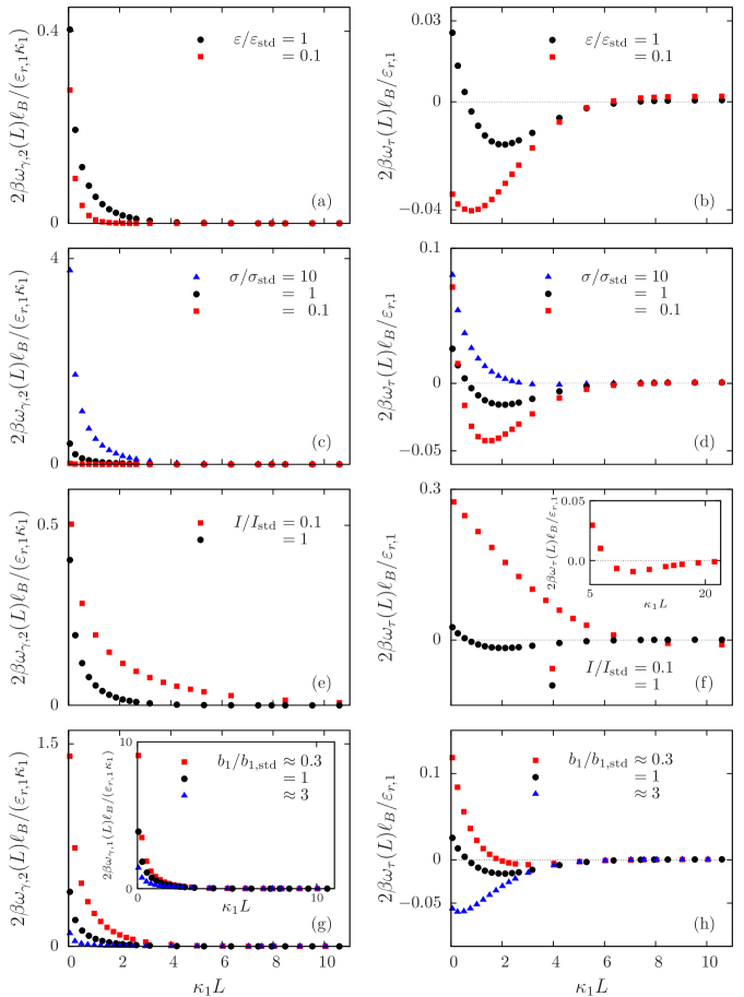
Figure 5: Left panels: Surface interaction energy $\omega_{\gamma,2}(L)$ per total area of the two walls in contact with medium “2” expressed in units of $\varepsilon_{r,1}\kappa_{1}/(2\beta\ell_{B})$ as a function of the rescaled wall separation $\kappa_{1}L$ for various sets of the free dimensionless parameters $\varepsilon$, $\sigma$, $I$, and $b_{1}$, respectively. Although $\omega_{\gamma,2}(L)$ is always repulsive, an increase in $\varepsilon$ or $\sigma$ strengthens the repulsion whereas an increase in $I$ or $b_{1}$ weakens it. Inset of panel (g): Scaled surface interaction energy per total area of the two walls in contact with medium “1” as a function of $\kappa_{1}L$. As one can infer from the plots, $\omega_{\gamma,1}$ and $\omega_{\gamma,2}$ behave similarly upon varying $b_{1}$. Right panels: Line interaction energy $\omega_{\tau}(L)$ per total length of the three-phase contact lines in units of $\varepsilon_{r,1}/(2\beta\ell_{B})$ as a function of $\kappa_{1}L$ for various sets of the dimensionless parameters. Compared with the standard set of parameters, the observed minimum of $\omega_{\tau}(L)$ becomes deeper and shifts towards smaller separations upon decreasing $\varepsilon$ or $\sigma$. The opposite trend occurs upon decreasing $I$ or $b_{1}$. The inset of panel (f) shows the variation of $\omega_{\tau}(L)$ for a larger range of $\kappa_{1}L$.

Within the linearized PB theory it is a common practice to use renormalized instead of bare surface charge densities in order to capture the correct asymptotic behavior of the electrostatic potential at large distances Boc02 . However, in the present study we are interested in the opposite limit of short distances. Still, it is interesting to see the effects of charge renormalization on $\omega_{\gamma,i}(L)$ and $\omega_{\tau}(L)$. This implies a replacement of the bare surface charge density ($\sigma_{i}$) with an effective charge density ($\pm\sigma_{\text{eff}}^{(i)}$) if $\sigma_{\text{eff}}^{(i)}<\lvert\sigma_{i}\rvert$. The analytic expression for the effective surface charge density is known for a single charged wall in contact with a semi-infinite electrolyte solution and is given by $\sigma_{\text{eff}}^{(i)}=e\kappa_{i}\varepsilon_{r,i}/(\pi\ell_{B})$, $i\in\{1,2\}$, with $\kappa(x>0)=\kappa_{1}$ and $\kappa(x<0)=\kappa_{2}$ Boc02 . For the above mentioned standard set of parameters, we have calculated separately $\sigma_{\text{eff}}^{(i)}$ for a single wall in contact with medium $i\in\{1,2\}$; it turns out that $\sigma_{\text{eff}}^{(1)}<\sigma_{1}$ whereas $\sigma_{\text{eff}}^{(2)}>\sigma_{2}$. Accordingly, we have only replaced $\sigma_{1}$ by $\sigma_{\text{eff}}^{(1)}$ keeping $\sigma_{2}$ the same. The corresponding results are presented in Fig. 3. As expected, both $\omega_{\gamma,1}(L)$ and $\omega_{\tau}(L)$ decrease in magnitude compared to the case of bare surface charge densities, but a significant quantitative mismatch compared with the full nonlinear behavior is still present. However, the results corresponding to the linear theory with bare or renormalized charge densities show the same qualitative behavior. Therefore, features like the minimum in Fig. 3(b) cannot be explained by simply using surface charge renormalization within the linear PB theory.

The strong reduction in strength of both the surface and the line parts raises the question concerning the relevance of the electrostatic interaction. In order to answer this, we compare our results with the van der Waals (vdW) interaction which is calculated in terms of the Hamaker constant Ham37 . For two flat surfaces made of polystyrene and interacting accross pure water, the Hamaker constant $A$ is reported to lie in the interval $[0.95,1.3]\times 10^{-20}\,\mathrm{J}$ Isr85 . Even for the maximal value of $A$, the vdW attraction energy $-A/(12\pi L^{2})$ per cross-sectional area due to the two surfaces is either comparable (for $L<2.5\,\mathrm{nm}$) or less by at least one order of magnitude compared to the corresponding electrostatic part. It is important to note that salting the water further decreases the vdW contribution slightly due to the electrostatic screening effect Isr85 . Therefore, the electrostatic part still contributes significantly to the total effective interaction. We are not aware of any such data regarding the line contribution to the interaction.

In the following we discuss the effects of varying the free parameters of our system. To this end, one of the five dimensionless parameters $\beta e\Phi_{D}$, $\varepsilon$, $\sigma$, $I$, or $b_{1}$ is varied at a time, keeping the remaining ones fixed. First, we consider the dimensionless Donnan potential $\beta e\Phi_{D}$. According to the linear theory Maj14 , all three $L$- dependent interaction energies, i.e., $\omega_{\gamma,1}(L)$, $\omega_{\gamma,2}(L)$, and $\omega_{\tau}(L)$, are independent of $\Phi_{D}$, which is confirmed by our numerical results. Moreover, this holds for the surface interactions $\omega_{\gamma,1}(L)$ and $\omega_{\gamma,2}(L)$ for arbitrary degrees $n$ of nonlinearity. In contrast, the line part $\omega_{\tau}(L)$ exhibits a completely different behavior (see Fig. 4). For $n=1$, $\omega_{\tau}(L)$ is attractive at all separations $L$ and independent of the value of $\Phi_{D}$. However, for $n\geq 2$ the line interaction $\omega_{\tau}(L)$ does depend on $\Phi_{D}$ (Fig. 4(b)). Starting from $n=4$, $\omega_{\tau}(L)$ hardly changes upon increasing the order of nonlinearity $n$. Figure 4(c) displays the corresponding results for $n=5$. For $\beta e\Phi_{D}\in\{-1,0\}$, $\omega_{\tau}(L)$ differs significantly in magnitude but it is repulsive everywhere, whereas for $\beta e\Phi_{D}=1$, which corresponds to its value in the standard set of parameters, it is repulsive at close separations $L$, but attractive further away. It is also worth noting that for $\beta e\Phi_{D}\in\{-1,0\}$, the predictions of the linear theory are qualitatively wrong at all separations $L$.

Effects of changing the remaining parameters $\varepsilon$, $\sigma$, $I$, and $b_{1}$ are shown in Fig. 5. Although here we present the results corresponding to the degree of nonlinearity $n=5$, for each set of parameters, the interaction energy curves basically do not change for $n\geq 4$. Therefore, in view of potential future studies, we conclude that it is sufficient to truncate the Taylor series in Eq. (6) at $n=4$. We change $\varepsilon$, $\sigma$, and $I$ by changing $\varepsilon_{2}$, $\sigma_{2}$, and $I_{2}$, respectively, while keeping their counterparts for medium “1” fixed. Consequently, $\omega_{\gamma,1}(L)$ does not change upon these variations; it changes only upon varying $b_{1}$. As shown by Fig. 5, although $\omega_{\gamma,2}(L)$ remains always repulsive (left column of panels), both its magnitude and its range depend on the above parameters. An increase in $\varepsilon$ or $\sigma$ strengthens the repulsion whereas an increase in $I$ or $b_{1}$ weakens the repulsion. The range of this repulsive energy is set by the Debye length (or equivalently the ionic strength) in medium “2”; for lower ionic strength the range increases. Upon changing $b_{1}$, $\omega_{\gamma,1}(L)$ behaves similarly as $\omega_{\gamma,2}(L)$ (see inset in Fig. 5(g)). Regarding the line interaction energy $\omega_{\tau}(L)$, the observed minimum for the standard set of parameters becomes deeper and shifts towards smaller separations upon decreasing $\varepsilon$ or $\sigma$. On the other hand, it becomes more shallow and shifts to a larger separation distance $L$ upon decreasing $I$ or $b_{1}$. Since in our system medium “2” is the less polar phase and since the standard values for $\varepsilon$ and $I$ are already close to unity, we do not have the option to increase these two quantities further. Nonetheless, the concomitant trends can be easily inferred from the data presented here.

What remains to be discussed is the relative importance of the line interaction $\omega_{\tau}$ as compared to the surface interactions $\omega_{\gamma,1}$ and $\omega_{\gamma,2}$. According to Eq. (6), the surface contributions scale with the area of the walls whereas the line contribution scales with the length of the three-phase contact lines. Hence, for sufficiently large surface area, the surface contributions eventually dominate. However, depending on the system parameters, the line contribution in Eq. (6) can dominate over the surface contributions even for typical sizes of the colloid particles. For example, we consider a generic system which consists of a water-lutidine (2,6-dimethylpyridine) mixture with NaI salt at temperature $T=313\,\mathrm{K}$, occupying the space between the two charged walls with an effective area $A_{i}=25\times 10^{4}\,\mathrm{nm^{2}}$ ($i\in\{1,2\}$). The effective length of the three-phase contact line is taken as $\ell=1000\,\mathrm{nm}$. The ionic concentration in the more polar water-rich phase is given by $I_{1}=0.1\,\mathrm{mM}$ and that for the less polar lutidine-rich phase is given by $I_{2}=0.085\,\mathrm{mM}$. The relative permittivities of the water- and lutidine-rich phases are given by $\varepsilon_{r,1}=72$ and $\varepsilon_{r,2}=62$, respectively. The walls carry a surface charge density of $\sigma_{1}=0.01\,e/\mathrm{nm^{2}}$ in contact with the water-rich phase and a surface charge density of $\sigma_{2}=0.0001\,e/\mathrm{nm^{2}}$ in contact with the lutidine-rich phase. Therefore the system is characterized by the following dimensionless parameters: $I=0.85$, $\sigma=0.01$, $\varepsilon=62/72$, $b_{1}=0.72$, and $\beta e\Phi_{D}=1$. For such a system, the line contribution for a wall separation $L\approx 90\,\mathrm{nm}$ (or $\kappa_{1}L\approx 3$), corresponding to the position of the minimum of $\omega_{\tau}$, is $\omega_{\tau}\ell\approx-27\,k_{B}T$, whereas the surface contributions are $\omega_{\gamma,1}A_{1}\approx 5\,k_{B}T$ and $\omega_{\gamma,2}A_{2}\approx 0.02\,k_{B}T$. Systems with other media are characterized by a different set of values for $\varepsilon$, $I$, and $\beta e\Phi_{D}$. For an oil with a smaller value of $\varepsilon_{r,2}$ the line interaction is expected to be more prominent because, with decreasing $\varepsilon$, $\omega_{\gamma,2}$ decreases whereas the minimum in $\omega_{\tau}$ becomes deeper (see Figs. 5(a) and (b)). The ratio $I$ can change in at least two ways: An increase of $I_{1}$ leads to a faster decay of $\omega_{\gamma,1}$ whereas a decrease of $I_{2}$ shifts the minimum of $\omega_{\tau}$ to larger values of $\kappa_{1}L$ (see Fig. 5(f)). Therefore, in both cases, the relative importance of the line interaction $\omega_{\tau}$ with respect to the surface interactions increases upon increasing $I$. An increase in the value of $\beta e\Phi_{D}$ will also deepen the minimum in $\omega_{\tau}$ leading to a stronger line interaction (see Fig. 4). It is important to note that $\omega_{\gamma,1}$ and $\omega_{\gamma,2}$ remain unaffected due to a change in the Donnan potential $\beta e\Phi_{D}$.

III.2 $L$-independent interactions

	analytical		numerical
			$n=1$	$n=2$	$n=3$	$n=4$	$n=5$
standard	$\gamma_{s,1}$	$=0.4398\,\ k_{\text{B}}T/\mathrm{nm^{2}}$	$0.4398$	$0.2992$	$0.2812$	$0.2781$	$0.2777$
	$\gamma_{s,2}$	$=0.01514\,\ k_{\text{B}}T/\mathrm{nm^{2}}$	$0.01514$	$0.01504$	$0.01504$	$0.01504$	$0.01504$
	$\gamma_{1,2}$	$=-0.002621\,\ k_{\text{B}}T/\mathrm{nm^{2}}$	$-0.002621$	$-0.002635$	$-0.002635$	$-0.002635$	$-0.002635$
	$\tau$	$=-0.5669\,\ k_{\text{B}}T/\mathrm{nm}$	$-0.5686$	$-0.06757$	$-0.03333$	$-0.02752$	$-0.02657$
$\beta e\Phi_{D}=0$	$\gamma_{s,1}$	$=0.4398\,\ k_{\text{B}}T/\mathrm{nm^{2}}$	$0.4398$	$0.2992$	$0.2812$	$0.2781$	$0.2777$
	$\gamma_{s,2}$	$=0.005141\,\ k_{\text{B}}T/\mathrm{nm^{2}}$	$0.005140$	$0.005037$	$0.005035$	$0.005035$	$0.005035$
	$\gamma_{1,2}$	$=0\,\ k_{\text{B}}T/\mathrm{nm^{2}}$	$0$	$0$	$0$	$0$	$0$
	$\tau$	$=-0.9509\,\ k_{\text{B}}T/\mathrm{nm}$	$-0.9520$	$-0.2655$	$-0.2067$	$-0.1963$	$-0.1947$
$\beta e\Phi_{D}=-1$	$\gamma_{s,1}$	$=0.4398\,\ k_{\text{B}}T/\mathrm{nm^{2}}$	$0.4398$	$0.2992$	$0.2812$	$0.2781$	$0.2777$
	$\gamma_{s,2}$	$=-0.004859\,\ k_{\text{B}}T/\mathrm{nm^{2}}$	$-0.004860$	$-0.004963$	$-0.004965$	$-0.004965$	$-0.004965$
	$\gamma_{1,2}$	$=-0.002621\,\ k_{\text{B}}T/\mathrm{nm^{2}}$	$-0.002621$	$-0.002635$	$-0.002635$	$-0.002635$	$-0.002635$
	$\tau$	$=-1.335\,\ k_{\text{B}}T/\mathrm{nm}$	$-1.3366$	$-0.5040$	$-0.4250$	$-0.4108$	$-0.4084$
$\varepsilon/\varepsilon_{\text{std}}=0.1$	$\gamma_{s,1}$	$=0.4398\,\ k_{\text{B}}T/\mathrm{nm^{2}}$	$0.4398$	$0.2992$	$0.2812$	$0.2781$	$0.2777$
	$\gamma_{s,2}$	$=0.0263\,\ k_{\text{B}}T/\mathrm{nm^{2}}$	$0.02624$	$0.02423$	$0.02406$	$0.02405$	$0.02404$
	$\gamma_{1,2}$	$=-0.001210\,\ k_{\text{B}}T/\mathrm{nm^{2}}$	$-0.001211$	$-0.001224$	$-0.001224$	$-0.001224$	$-0.001224$
	$\tau$	$=-0.1401\,\ k_{\text{B}}T/\mathrm{nm}$	$-0.1424$	$0.009198$	$0.01742$	$0.01876$	$0.01899$
$\sigma/\sigma_{\text{std}}=10$	$\gamma_{s,1}$	$=0.4398\,\ k_{\text{B}}T/\mathrm{nm^{2}}$	$0.4398$	$0.2992$	$0.2812$	$0.2781$	$0.2777$
	$\gamma_{s,2}$	$=0.6141\,\ k_{\text{B}}T/\mathrm{nm^{2}}$	$0.6140$	$0.4317$	$0.4081$	$0.4037$	$0.4030$
	$\gamma_{1,2}$	$=-0.002621\,\ k_{\text{B}}T/\mathrm{nm^{2}}$	$-0.002621$	$-0.002635$	$-0.002635$	$-0.002635$	$-0.002635$
	$\tau$	$=-0.1127\,\ k_{\text{B}}T/\mathrm{nm}$	$-0.1133$	$-0.07228$	$-0.07077$	$-0.07052$	$-0.07046$
$\sigma/\sigma_{\text{std}}=0.1$	$\gamma_{s,1}$	$=0.4398\,\ k_{\text{B}}T/\mathrm{nm^{2}}$	$0.4398$	$0.2992$	$0.2812$	$0.2781$	$0.2777$
	$\gamma_{s,2}$	$=0.001051\,\ k_{\text{B}}T/\mathrm{nm^{2}}$	$0.001051$	$0.001051$	$0.001051$	$0.001051$	$0.001051$
	$\gamma_{1,2}$	$=-0.002621\,\ k_{\text{B}}T/\mathrm{nm^{2}}$	$-0.002621$	$-0.002635$	$-0.002635$	$-0.002635$	$-0.002635$
	$\tau$	$=-0.7615\,\ k_{\text{B}}T/\mathrm{nm}$	$-0.7634$	$-0.1469$	$-0.09980$	$-0.09171$	$-0.09039$
$I/I_{\text{std}}=0.1$	$\gamma_{s,1}$	$=0.4398\,\ k_{\text{B}}T/\mathrm{nm^{2}}$	$0.4396$	$0.2988$	$0.2808$	$0.2777$	$0.2772$
	$\gamma_{s,2}$	$=0.02626\,\ k_{\text{B}}T/\mathrm{nm^{2}}$	$0.02626$	$0.02425$	$0.02409$	$0.02407$	$0.02407$
	$\gamma_{1,2}$	$=-0.001210\,\ k_{\text{B}}T/\mathrm{nm^{2}}$	$-0.001210$	$-0.001223$	$-0.001223$	$-0.001223$	$-0.001223$
	$\tau$	$=-0.4251\,\ k_{\text{B}}T/\mathrm{nm}$	$-0.4283$	$-0.2093$	$-0.1973$	$-0.1957$	$-0.1954$
$b_{1}/b_{1,\text{std}}\approx 3$	$\gamma_{s,1}$	$=0.1391\,\ k_{\text{B}}T/\mathrm{nm^{2}}$	$0.1391$	$0.1251$	$0.1241$	$0.1240$	$0.1240$
	$\gamma_{s,2}$	$=0.01163\,\ k_{\text{B}}T/\mathrm{nm^{2}}$	$0.01163$	$0.01162$	$0.01162$	$0.01162$	$0.01162$
	$\gamma_{1,2}$	$=-0.008287\,\ k_{\text{B}}T/\mathrm{nm^{2}}$	$-0.008288$	$-0.008332$	$-0.008332$	$-0.008332$	$-0.008332$
	$\tau$	$=0.02634\,\ k_{\text{B}}T/\mathrm{nm}$	$0.02573$	$0.03243$	$0.03284$	$0.03287$	$0.03287$
$b_{1}/b_{1,\text{std}}\approx 0.3$	$\gamma_{s,1}$	$=1.391\,\ k_{\text{B}}T/\mathrm{nm^{2}}$	$1.391$	$0.6061$	$0.5098$	$0.4860$	$0.4798$
	$\gamma_{s,2}$	$=0.02626\,\ k_{\text{B}}T/\mathrm{nm^{2}}$	$0.02626$	$0.02425$	$0.02408$	$0.02407$	$0.02407$
	$\gamma_{1,2}$	$=-0.0008287\,\ k_{\text{B}}T/\mathrm{nm^{2}}$	$-0.0008288$	$-0.0008332$	$-0.0008332$	$-0.0008332$	$-0.0008332$
	$\tau$	$=-8.295\,\ k_{\text{B}}T/\mathrm{nm}$	$-8.305$	$-0.4430$	$-0.1653$	$-0.1129$	$-0.09931$

Table 1: Values of the surface tensions $\gamma_{s,1}$ and $\gamma_{s,2}$ at the walls in contact with medium “1” and “2”, respectively, interfacial tension $\gamma_{1,2}$, and line tension $\tau$ at the three-phase contact lines for various sets of parameters $\varepsilon$, $\sigma$, $I$, and $b_{1}$. The second column provides the values for the linearized theory calculated by using Eqs. (7)–(9). The remaining columns provide the values corresponding to various orders of the nonlinearity $n$ considered in Eq. (5). As expected, the values for $n=1$ agree well with the analytical results. For higher orders $n$ of the nonlinearity, the magnitudes of the surface tensions $\gamma_{s,i}$ decrease noticeably, whereas the absolute value of the interfacial tension $\gamma_{1,2}$ increases slightly. However, the quantity, which is most sensitive with respect to $n$, is the line tension $\tau$. In some cases it exhibits variations of several orders of magnitude as function of $n$; upon increasing the degree of nonlinearity $n$ it can increase, decrease, or even change sign. For $n\geq 4$ the dependences on $n$ level off.

In this subsection we discuss the remaining, $L$-independent contributions $\gamma_{s,i}$, $\gamma_{1,2}$, and $\tau$ in Eq. (6). Analytical expressions for these quantities can be obtained within linear theory (i.e., degree of nonlinearity $n=1$), following the same procedure as the one presented in Ref. Maj14 :

$$\gamma_{s,i} =\frac{\sigma_{i}^{2}}{2\kappa_{i}\varepsilon_{i}}+\sigma_{i}\Phi_{b},\qquad i\in\{1,2\},$$ (7)

$$\gamma_{1,2} =-\frac{\kappa_{1}\kappa_{2}\varepsilon_{1}\varepsilon_{2}\Phi_{D}^{2}}{\kappa_{1}\varepsilon_{1}+\kappa_{2}\varepsilon_{2}},$$ (8)

and

$$\tau=\!\left(\frac{\Phi_{D}}{1+\kappa\varepsilon}\right)\!\!\left(\frac{\kappa\varepsilon\sigma_{1}}{\kappa_{1}}-\frac{\sigma_{2}}{\kappa_{2}}\right)\!\!-\!\frac{\sigma_{1}^{2}}{\kappa_{1}^{2}\varepsilon_{1}}\!\int\limits_{0}^{\infty}\!dx\!\bigg{[}\frac{\frac{\sigma}{\varepsilon}\frac{1}{x^{2}\pi^{2}+\kappa^{2}}\!-\!\frac{1}{x^{2}\pi^{2}+1}}{1\!+\!\frac{\sqrt{x^{2}\pi^{2}+1}}{\varepsilon\sqrt{x^{2}\pi^{2}+\kappa^{2}}}}\frac{1}{\sqrt{x^{2}\pi^{2}+1}}+\frac{\frac{\sigma}{x^{2}\pi^{2}+1}\!-\!\frac{\sigma^{2}}{\varepsilon}\frac{1}{x^{2}\pi^{2}+\kappa^{2}}}{1\!+\!\frac{\varepsilon\sqrt{x^{2}\pi^{2}+\kappa^{2}}}{\sqrt{x^{2}\pi^{2}+1}}}\frac{1}{\sqrt{x^{2}\pi^{2}+\kappa^{2}}}\bigg{]},$$ (9)

where $\varepsilon_{i}=\varepsilon_{r,i}\varepsilon_{0}$, $i\in\{1,2\}$ and $\kappa=\kappa_{2}/\kappa_{1}$. In Table I the values resulting from these expressions along with the ones obtained numerically are listed for each set of parameters. As one can see, the numerical values for $n=1$ (3rd column) agree well with the analytical results (2nd column). Whereas the values vary as functions of the degree of nonlinarity $n$, they do not change significantly for $n\geq 4$. For weaker interactions (e.g., in the less polar phase) this convergence is even more rapid. In line with the $L$-dependent interactions $\omega_{s,i}(L)$, the magnitudes of the surface tensions $\gamma_{s,i}$ decrease upon increasing the degree of nonlinearity $n$. On the other hand, the absolute value of the interfacial tension $\gamma_{1,2}$ increases slightly with increasing order of nonlinearity $n$ and, as expected, it is independent of the surface charge densities at the walls. For an ionic strength of $1\,\mathrm{mM}$ in the aqueous phase, the predicted values for the interfacial tension also agrees well with those obtained in earlier studies Gue39 ; Bie08 . In contrast, the line tension $\tau$ is most sensitive to the degree of nonlinearity. Depending on the values chosen for the free parameters, $\tau$ can either increase or decrease with increasing $n$; in some cases (e.g., for $b_{1}/b_{1,\text{std}}\approx 0.3$) it varies by two orders of magnitude upon increasing $n$. For $\varepsilon/\varepsilon_{\text{std}}=0.1$, it even changes sign due to the presence of the nonlinearity. The values for our expressions for the line tension $\tau$ are either of the order of $1\,\mathrm{pN}$ or slightly less, which is consistent with values reported in the literature Bre98 ; Get98 ; Bau99 ; Pom00 ; Mug02 . By considering variations of the parameter $b_{1}$ it can be inferred from Tab. I that the line tension $\tau$ increases upon increasing the ionic strength $I$. This is not in contradiction to the decrease of $\tau$ upon increasing $I$ close to a wetting transition, as reported in Ref. Iba16 : In fact, in that study only contact angles of $<50^{\circ}$ occurred, and the observed decrease of $\tau$ upon increasing the ionic strength $I$ has been found to become smaller for increasing contact angles (Fig. 5(b) in Ref. Iba16 ); in contrast, in the present study there are no wetting transitions and the contact angle is large, i.e., $90^{\circ}$.

IV Conclusion

Within the framework of nonlinear Poisson-Boltzmann theory, we have addressed the issue regarding the electrostatic interaction between a pair of identical, charged walls at distance $L$, separated by two immiscible electrolyte solutions forming a flat interface (Fig. 1). Our numerical findings demonstrate that for small $L$ the linear theory overestimates all $L$-dependent contributions to the total electrostatic interaction by at least one order of magnitude (Fig. 2). Within the nonlinear theory the qualitative trends of the effective surface and line interaction potentials as functions of all system parameters have been discussed (Figs. 4 and 5). Whereas the variations as functions of the degree $n$ of nonlinearity of the surface and interfacial contributions (i.e., the surface interaction energy, the surface tension, and the interfacial tension) are only of a quantitative character, the line contributions (line interaction energy and line tension) show a qualitatively different behavior within the nonlinear theory as compared to the corresponding predictions of the linear theory (Figs. 2, 4, 5 and Tab. I). For example, while the linear theory predicts a monotonically decreasing, attractive interaction between the two three-phase contact lines, nonlinearity changes it to a repulsive one at close separations which turns attractive at large distances $L$ (Figs. 2(e) and (f)). These differences between the linear and the nonlinear theory cannot be explained by using, within the linear theory, a simple charge renormalization procedure (Fig. 3). Depending on the parameters, the line tension is found to change sign (Tab. I). Moreover, a dependence of the line interaction energy on the solvation properties of the two media (described in terms of the Donnan potential) is present only within the nonlinear theory (Fig. 4). The degree of nonlinearity is given by truncating the series expansion of the right-hand side of the Poisson-Boltzmann equation (3). The ensuing results indicate that it is sufficient to consider only the first few terms in this series. The system we have studied is expected to mimic the situation of two colloidal particles being trapped very close to each other at a liquid interface. Depending on the interaction among each other, particles are known to form stable, unstable, or even mesostructures at a liquid interface Bin06 . In the unstable situation, particles aggregate to form fractal structures. Whereas for a stable monolayer to form, long-ranged interactions between the particles are required. On the other hand, the formation of fractal structures requires the total interaction potential to be short-ranged and characterized by a minimum at very short distances. Accordingly, our findings are particularly relevant with respect to this aspect. Thus, we expect our results for a pair of colloids to contribute towards a better understanding of the formation and stability of many-body colloidal monolayers trapped at fluid interfaces.

References

- (1) W. Ramsden, Proc. R. Soc. London 72, 156 (1903).
- (2) E. Dickinson, Colloids Surf. 42, 191 (1989).
- (3) D. E. Tambe and M. M. Sharma, Adv. Colloid Interface Sci. 52, 1 (1994).
- (4) A. D. Dinsmore, M. F. Hsu, M. G. Nikolaides, M. Márquez, A. R. Bausch, and D. A. Weitz, Science 298, 1006 (2002).
- (5) B. P. Binks and T. S. Horozov, Colloidal Particles at Liquid Interfaces (Cambridge University Press, Cambridge, 2006).
- (6) M. G. Nikolaides, A. R. Bausch, M. F. Hsu, A. D. Dinsmore, M. P. Brenner, C. Gay, and D. A. Weitz, Nature 420, 299 (2002).
- (7) L. Foret and A. Würger, Phys. Rev. Lett. 92, 058302 (2004).
- (8) M. Oettel, A. Domínguez, and S. Dietrich, Phys. Rev. E 71, 051401 (2005).
- (9) M. Oettel and S. Dietrich, Langmuir 24, 1425 (2008).
- (10) P. Pieranski, Phys. Rev. Lett. 45, 569 (1980).
- (11) A. J. Hurd, J. Phys. A 18, L1055 (1985).
- (12) R. Aveyard, J. H. Clint, D. Nees, and V. N. Paunov, Langmuir 16, 1969 (2000).
- (13) R. Aveyard, B. P. Binks, J. H. Clint, P. D. I. Fletcher, T. S. Horozov, B. Neumann, V. N. Paunov, J. Annesley, S. W. Botchway, D. Nees, A. W. Parker, A. D. Ward, and A. N. Burgess, Phys. Rev. Lett. 88, 246102 (2002).
- (14) T. S. Horozov and B. P. Binks, Colloids Surf. A 267, 64 (2005).
- (15) B. J. Park, J. P. Pantina, E. M. Furst, M. Oettel, S. Reynaert, and J. Vermant, Langmuir 24, 1686 (2008).
- (16) A. Toor, T. Feng, and T. P. Russell, Eur. Phys. J. E 39, 57 (2016).
- (17) A. Majee, M. Bier, and S. Dietrich, J. Chem. Phys. 140, 164906 (2014).
- (18) D. Frydel, S. Dietrich, and M. Oettel, Phys. Rev. Lett. 99, 118302 (2007).
- (19) W. B. Russell, D. A. Saville, and W. R. Schowalter, Colloidal Dispersions (Cambridge University Press, Cambridge, 1989).
- (20) M. P. Lyne, B. D. Bowen, and S. Levine, J. Colloid Interface Sci. 150, 374 (1992).
- (21) R. Aveyard, B. P. Binks, and J. H. Clint, Adv. Colloid Interface Sci. 100, 503 (2003).
- (22) F. Reincke, S. G. Hickey, W. K. Kegel, and D. Vanmaekelbergh, Angew. Chem. Int. Ed. 43, 458 (2004).
- (23) K. Masschaele, B. J. Park, E. M. Furst, J. Fransaer, and J. Vermant, Phys. Rev. Lett. 105, 048303 (2010).
- (24) R. Evans, Adv. Phys. 28, 143 (1979).
- (25) M. Bier, A. Gambassi, and S. Dietrich, J. Chem. Phys. 137, 034504 (2012).
- (26) V. S. Bagotsky, Fundamentals of Electrochemistry (Wiley, Hoboken, NJ, 2006).
- (27) R. W. Rampolla and C. P. Smyth, J. Am. Chem. Soc. 80, 1057 (1958).
- (28) P. D. Gallagher, M. L. Kurnaz, and J. V. Maher, Phys. Rev. A 46, 7750 (1992).
- (29) C. A. Grattoni, R. A. Dawe, C. Y. Seah, and J. D. Gray, J. Chem. Eng. Data 38, 516 (1993).
- (30) H. D. Inerowicz, W. Li, and I. Persson, J. Chem. Soc. Faraday Trans. 90, 2223 (1994).
- (31) D. R. Lide, Handbook of Chemistry and Physics, 82nd ed. (CRC, Boca Raton, 20012002).
- (32) L. Bocquet, E. Trizac, and M. Aubouy, J. Chem. Phys. 117, 8138 (2002).
- (33) H. C. Hamaker, Physica 4, 1058 (1937).
- (34) J. N. Israelachvili, Intermolecular and Surface Forces (Academic Press, New York, 2011).
- (35) W. L. Guest and W. C. M. Lewis, Proc. R. Soc. London 170, 501 (1939).
- (36) M. Bier, J. Zwanikken, and R. van Roij, Phys. Rev. Lett. 101, 046104 (2008).
- (37) F. Bresme and N. Quirke, Phys. Rev. Lett. 80, 3791 (1998).
- (38) T. Getta and S. Dietrich, Phys. Rev. E 57, 655 (1998).
- (39) C. Bauer and S. Dietrich, Eur. Phys. J. B 10, 767 (1999).
- (40) T. Pompe and S. Herminghaus, Phys. Rev. Lett. 85, 1930 (2000).
- (41) F. Mugele, T. Becker, R. Nikopoulos, M. Kohonen, and S. Herminghaus, J. Adhesion Sci. Technol. 16, 951 (2002).
- (42) I. Ibagon, M. Bier, and S. Dietrich, J. Phys.: Condens. Matter 28, 244015 (2016).