Dissipation assisted quantum correlations in coupled qubits

Abstract

We theoretically investigate a possibility to establish multi-qubit quantum correlations in one-dimensional chains of qubits. We combine a reservoir engineering strategy with coherent dynamics to generate multi-qubit entangled states. We find that an interplay between the coherent and incoherent dynamics result in the generation of stable (time-independent) many-body entangled steady states. Our results will be relevant in the context of the dissipative generation of quantum states, with applications in short-distance quantum computation and for exploring the emergence of collective phenomena in many-body open quantum systems.

I Introduction

Quantum technology promises novel techniques to process information at a level and scale which is inconceivable in the classical domain aste98 ; chbe00 . Technological advancements in the past two decades have fueled the transformation of early theoretical ideas and protocols highlighting quantum weirdness into experimental reality shar13 ; djwi13 . Over the years, different quantum systems have received growing attention for exploring them in various roles, including quantum simulators rfey82 ; dporr04 ; kkim11 ; rbla12 ; imge14 and processors for various tasks in quantum computation and information tdla10 . Unfortunately, almost every quantum system, that is of potential interest to us, also irreversibly couples to its external environment. This normally leads to decoherence and dissipation in quantum systems whzu03 . It is, therefore, advisable to minimize the influence of reservoir induced decoherence on a quantum system. In this direction, quantum control strategies have taken a center stage for quantum state protection in noisy quantum systems (see arrrc01 ; bmte15 ; csay11 ; kfui14 ; jkel15 ; sjgl15 ; yliu16 ; cjosh16 , and references therein).

Somewhat counterintuitively, it is also possible to engineer the irreversible system-reservoir coupling in order to prepare desired many-body quantum states sdie08 ; fver09 ; hkra11 ; jtba11 ; ylin13 ; tram14 . These schemes are based on the method of reservoir engineering jfpo96 to tailor the system-reservoir coupling and drive the quantum system to a desired quantum state. In this work, we follow one such reservoir engineering strategy considered in sdie08 ; jtba11 and combine it with coherent interactions to create stable many-body quantum states. Prime motivation behind our work is our shared belief that the influence of environment induced dissipation can also be particularly intriguing when the quantum system of interest itself is already an interacting many-body system. In such a scenario, an interesting interplay between the coherent and incoherent interactions can result in the generation of non-trivial many-body states with applications in quantum technologies sdie08 ; fver09 ; hkra11 ; jtba11 ; ylin13 ; tram14 ; cchen16 .

In this work, we will specifically focus on one-dimensional chains of two-level systems (or, “qubits”) to engineer stable quantum many-body states. The prospects of using qubit chains as “non-photonic” alternates for short distance quantum communication has already received considerable attention in the past sbos03 ; sbos07 ; akay10 . These strategies exploit the inter-qubit coherent interactions to accomplish some of the necessary tasks in quantum computation and information processing. Specific applications include “quantum interconnects” to join two or more quantum processors, “quantum channels” for quantum state transfer and entanglement generation between distant qubits sbos03 ; sbos07 ; akay10 ; idam07 ; mchr04 ; lami08 ; tscu08 ; cdfr08 ; nyya11 ; lban11 ; fcar14 ; ssah15 ; rjch16 . In contrast to previous proposals, our current agenda will be to combine the ideas from reservoir engineering with coherent dynamics between the qubits to create time-independent many-body quantum states. Specifically, we will use the method of reservoir engineering to create a two-qubit entangled state. This dissipatively generated entangled state, evolving under competing coherent interactions, transforms to yield a multi-qubit entangled state.

The open dynamics of an interacting many-body open quantum system can often be well described by a Lindblad type master equation under the Born-Markov and secular approximations hpbr02 ,

$$\dot{\hat{\rho}}=-i[\hat{H}_{\rm S},\hat{\rho}]+\Gamma\hat{\mathcal{L}}_{\hat{A}}\hat{\rho},$$ (1)

where $\hat{\rho}$ is the system’s state, $\hat{H}_{\rm S}$ is the system Hamiltonian, and $\hat{\mathcal{L}}_{\hat{A}}\hat{\rho}$ is the Lindblad super operator rendering the effects of the reservoir on the system ($\hat{A}$ is the so called quantum jump operator). The steady state is solved by letting $i[\hat{H}_{\rm S},\hat{\rho}_{\mathrm{ss}}]-\Gamma\hat{\mathcal{L}}_{\hat{A}}\hat{\rho}_{\mathrm{ss}}=0$. In the sections to follow next, we will show that a carefully designed reservoir coupling when combined with coherent evolution can indeed result in such stable (time-independent) many-body quantum states.

II Model: two qubits

We begin with considering a physical system composed of two qubits with their closed dynamics governed by a Hamiltonian of the form ($\hbar=1$),

$$\hat{H}_{\rm P}=\Delta(\hat{\sigma}_{1}^{z}+\hat{\sigma}_{2}^{z}),$$ (2)

where $\Delta$ is the (identical) energy level splitting between the two energy levels of each qubit. Throughout in this paper we will use dimensionless parameters such that we will scale all frequencies by $\Delta$ and time by $\Delta^{-1}$. Nevertheless, we will keep $\Delta$ in all expressions and will always use $\Delta=1$ in any calculations. For reasons that will soon become clear, the two qubits evolving under the Hamiltonian (2) form what we call the primary chain, and this is reflected in our choice of notation $\hat{H}_{\rm P}$ in equation (2). We start with revisiting a reservoir engineering strategy originally proposed in sdie08 and experimentally realized in a linear ion-trap quantum computer architecture in jtba11 . We, thus, envision an open version scenario where the two qubits in the primary chain are also coupled to an engineered reservoir,

$$\dot{\hat{\rho}}=-i[\hat{H}_{\rm P},\hat{\rho}]+\Gamma\hat{\mathcal{L}}_{{\hat{b}}_{1,2}}\hat{\rho},$$ (3)

where ${\hat{b}}_{1,2}=(\hat{\sigma}_{1}^{+}+\hat{\sigma}_{2}^{+})(\hat{\sigma}_{1}^{-}-\hat{\sigma}_{2}^{-})$ is the bi-local quantum jump operator sdie08 ; jtba11 . As discussed in detail in Refs. sdie08 ; jtba11 , the above quantum jump operator map any antisymmetric component in the wavefunction on a pair of qubits into the symmetric one. We refer the reader to jtba11 for a physical realization of the above quantum jump operator in trapped atomic ions. In order to understand the role of the bi-local quantum jump operator in the above master equation (3), we assume that the two qubits are initialized in a pure state $|\psi(0)\rangle=|\uparrow\rangle_{1}|\downarrow\rangle_{2}$ with zero angular momentum projection along the $z$ direction. The bi-local operator ${\hat{b}}_{1,2}$ acting on this initial gives ${\hat{b}}_{1,2}|\uparrow\rangle_{1}|\downarrow\rangle_{2}=|\uparrow\rangle_{1}|\downarrow\rangle_{2}+|\downarrow\rangle_{1}|\uparrow\rangle_{2}=|\Psi^{+}\rangle$. The projector $|\Psi^{+}\rangle\langle\Psi^{+}|$ also commutes with the two-qubit Hamiltonian (2) and, therefore, the two qubits evolving under the master equation (3) reach a pure steady state $\rho\sim|\Psi^{+}\rangle\langle\Psi^{+}|$. It is worth pointing out that in the absence of non-zero direct coupling between the qubits in the primary chain, the creation of a maximally entangled pure state $|\Psi^{+}\rangle$ crucially depends on the initial state $|\psi(0)\rangle$. Symmetric initial states $|\downarrow\rangle_{1}|\downarrow\rangle_{2},|\uparrow\rangle_{1}|\uparrow\rangle_{2}$ are the stationary states of the master equation (3).

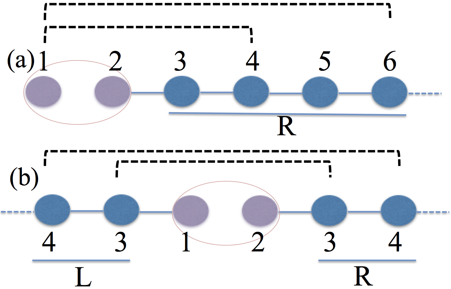
Figure 1: (Color online) (a) The primary two-qubit chain is coupled to the secondary chain of qubits on its “right”. The goal is to prepare a many-body quantum state exhibiting steady state correlations between the 1^st and $n^{\rm th}$ qubits (joined in dashed). (b) The primary two-qubit chain is situated in the “center” and is connected to the two secondary chains on its “left” and “right” respectively. The goal is to establish bi-partite correlations between the qubits placed at the remote (open) ends of the two secondary chains (joined in dashed). In both these configurations the primary qubits are assumed to couple to a common engineered reservoir, with no direct coupling between them.

III Model: many qubits

We now consider physical scenarios where additional (secondary) chains of coupled qubits are joined with the two-qubit primary chain in two different spatial configurations, as shown in Fig.1. In what follows next, we will explore the open dynamics of the coupled qubits of the primary and secondary chains arranged in these two different geometries.

III.1 Qubit chain: geometry (a)

We start with describing the evolution of the qubits in the primary and secondary chains, arranged as shown in Fig.1(a). We model the closed dynamics of these coupled qubits under the following Hamiltonian,

$$\hat{H}_{\rm P-S}^{\rm a}=\hat{H}_{\rm P}+\hat{H}_{\rm S}^{\rm{R}}+\hat{H}_{\rm cplng}^{\rm P-R},$$ (4)

where $\hat{H}_{\rm P}$, given by equation (2), describes the evolution of the two qubits in the primary chain. The secondary chain which is coupled to the primary chain on its “right” is modeled as a collection of coupled qubits under a Hamiltonian,

$$\hat{H}_{\rm S}^{\rm R}=\sum_{j=3,4...}\Delta\hat{\sigma}_{j,{\rm R}}^{z}+\kappa(\hat{\sigma}_{j,\rm{R}}^{+}\hat{\sigma}_{j+1,\rm{R}}^{-}+h.c.),$$ (5)

where $\hat{\sigma}_{j,{\rm R}}^{z}$ represents the Pauli-$z$ operator of the $j^{\rm th}$ qubit in the secondary chain and the inter-qubit coupling strength is denoted by $\kappa$. The coherent coupling between the primary and secondary chains is assumed to take a form,

$$\hat{H}_{\rm cplng}^{\rm P-R}=\theta(\hat{\sigma}_{2}^{+}\hat{\sigma}_{3,\rm{R}}^{-}+h.c),$$ (6)

where $\theta$ is the inter-chain coupling strength. In the discussion to follow next, we will fix $\theta=\kappa$.

We now use a following strategy to achieve quantum many-body states of qubits in the primary and secondary chains. We assume that the qubits in the secondary chain remain decoupled from the external surroundings and the qubits in the primary chain couple to an engineered reservoir through the action of the bi-local quantum jump operator ${\hat{b}}_{1,2}$. The qubits in the secondary chain can be protected from external noisy environment through a quantum control strategy such as dynamical decoupling. The idea behind dynamical decoupling is to rapidly rotate the quantum system by means of classical fields in order to average the system-environment coupling to zero gdel10 ; aber12 ; nbar13 . The collective open dynamics of the qubits in the primary and secondary chains can then be modeled by a master equation of the form,

$$\dot{\hat{\rho}}=-i[\hat{H}_{\rm P-S}^{\rm a},\hat{\rho}]+\Gamma\hat{\mathcal{L}}_{{\hat{b}}_{1,2}}\hat{\rho}.$$ (7)

It is easy to verify that the evolution under the master equation (7) conserves the initial number of excitations present in the primary and secondary chains. We, therefore, initialize the qubits in a non-vacuum state. Specifically, we assume that the qubits in the primary chain are initially in a state $|\psi(0)\rangle=|\uparrow\rangle_{1}|\downarrow\rangle_{2}$ and all qubits in the secondary chain are initialized in their ground states $|\psi_{j,R}(0)\rangle=|\downarrow\rangle_{j}~{}(j=3,4...)$. Our claim is, this initial state, evolving under the master equation (7), will evolve to a pure many-body entangled state of the primary and secondary qubits. In order to show this, we first numerically simulate the master equation (7) and then provide an analytical explanation for the results. We simulate the master equation (7) for even number of qubits ($2N$) in the secondary chain. Therefore, the total number of qubits in the primary and secondary chains is $n=2+2N~{}(N=1,2,3...)$. We use the method of time evolving block decimation (TEBD) extended to open systems (mixed states) mzwo04 to numerically simulate our many-body master equation (7). This numerical method has been previously applied to explore non-equilibrium features in driven-dissipative many-body quantum systems cjosh13 . Our numerical approach allows us to compute single- and double- site correlators, which is suffice to reconstruct the reduced density matrix of any two qubits in the primary and secondary chains.

In Fig.2(a), we plot the steady state correlator $|\langle\hat{\sigma}_{1}^{+}\hat{\sigma}_{j}^{-}\rangle|$ as a function of index $j$. This captures the degree of pairwise correlations present between the first qubit in the primary chain and all other qubits, arranged as shown in Fig.1(a). We have now dropped the subscript “R” in the Pauli raising and lowering operators for the qubits in the secondary chain. One interesting observation from Fig.2(a) is that the steady state correlator $|\langle\hat{\sigma}_{1}^{+}\hat{\sigma}_{j}^{-}\rangle|$ for coupled qubits’ arrangement of Fig.1(a) follow a pattern,

$$|\langle\hat{\sigma}_{1}^{+}\hat{\sigma}_{j}^{-}\rangle| = 0,{\rm when}~{}j\in{\rm odd},$$

$$|\langle\hat{\sigma}_{1}^{+}\hat{\sigma}_{j}^{-}\rangle| = {\rm constant},{\rm when}~{}j\in{\rm even},$$

where the value of the constant depends only on the total number of qubits $n$ in the chain and is completely independent of $j$. Furthermore, from the numerical solution of the master equation (7) we find that $\langle\hat{\sigma}_{j}^{z}\rangle=-1~{}\forall~{}j\in{\rm odd}~{}(j=3,5,7...)$, while $\langle\hat{\sigma}_{j}^{z}\rangle~{}(j=1,2,4...)$ depends on the total number of qubits $n$ in the chain (see below). The TEBD method provides an efficient way to simulate our many-body master equation (7), but we do not have access to the full steady state density matrix itself. Therefore, we numerically diagonalize the master equation (7) for small values of $n$ to gain more insight into the steady state of the master equation (7) and the correlation pattern of Fig.2(a). For example, an exact numerical diagonalization of the master equation (7) for $n=4$ result in a following pure steady state,

$$|\Psi_{\rm n=4}\rangle = \frac{1}{\sqrt{3}}(|\uparrow\rangle_{1}|\downarrow\rangle_{2}|\downarrow\rangle_{4}+|\downarrow\rangle_{1}|\uparrow\rangle_{2}|\downarrow\rangle_{4}$$ (8)

$$-|\downarrow\rangle_{1}|\downarrow\rangle_{2}|\uparrow\rangle_{4})\otimes|\downarrow\rangle_{3}.$$

It is easy to verify that $|\Psi_{\rm n=4}\rangle$ is an eigenstate of the Hamiltonian $\hat{H}_{\rm P-S}^{\rm a}$ (4) and, thus, the corresponding steady state $\hat{\rho}_{\rm n=4}~{}(|\Psi_{\rm n=4}\rangle\langle\Psi_{\rm n=4}|)$ commutes with the Hamiltonian $\hat{H}_{\rm P-S}^{\rm a}$. Moreover, the state $\hat{\rho}_{\rm n=4}$ is also a symmetric state of the qubits in the primary chain (qubits 1 and 2) and, therefore, also a dark state of the bi-local Lindblad operators $\hat{\mathcal{L}}_{{\hat{b}}_{1,2}}\hat{\rho}_{\rm n=4}$. It is quite remarkable to observe that the steady state solutions $\hat{\rho}_{\rm n=4}$ is independent of the inter-qubit and inter-chain coupling strengths. Of course, these coupling strength determine the time scale for the production of the steady state $\hat{\rho}_{\rm n=4}$. It is immediately clear that the state (8) is similar to a three-qubit $W$ state, except for the weighting factors. Such a $W$ state represent one of the two entangled classes of three-qubit states with several applications in quantum information theory, the other being the $GHZ$ states wdur00 ; vngo06 ; bookchuang . $W$ states have interesting properties, including a non-zero bi-partite entanglement between any pair of qubits and robustness of quantum correlations against loss of one qubit. Likewise, through a direct numerical diagonalization of the master equation (7) we obtain following pure steady states,

$$|\Psi_{\rm n=6}\rangle = \frac{1}{\sqrt{4}}(|\uparrow\rangle_{1}|\downarrow\rangle_{2}|\downarrow\rangle_{4}|\downarrow\rangle_{6}+|\downarrow\rangle_{1}|\uparrow\rangle_{2}|\downarrow\rangle_{4}|\downarrow\rangle_{6}$$ (9)

$$-|\downarrow\rangle_{1}|\downarrow\rangle_{2}|\uparrow\rangle_{4}|\downarrow\rangle_{6}+|\downarrow\rangle_{1}|\downarrow\rangle_{2}|\downarrow\rangle_{4}|\uparrow\rangle_{6})$$

$$\otimes|\downarrow\rangle_{3}|\downarrow\rangle_{5},$$

$$|\Psi_{\rm n=8}\rangle = \frac{1}{\sqrt{5}}(|\uparrow\rangle_{1}|\downarrow\rangle_{2}|\downarrow\rangle_{4}|\downarrow\rangle_{6}|\downarrow\rangle_{8}+|\downarrow\rangle_{1}|\uparrow\rangle_{2}|\downarrow\rangle_{4}$$ (10)

$$|\downarrow\rangle_{6}|\downarrow\rangle_{8}-|\downarrow\rangle_{1}|\downarrow\rangle_{2}|\uparrow\rangle_{4}|\downarrow\rangle_{6}|\downarrow\rangle_{8}+|\downarrow\rangle_{1}|\downarrow\rangle_{2}$$

$$|\downarrow\rangle_{4}|\uparrow\rangle_{6}|\downarrow\rangle_{8}-|\downarrow\rangle_{1}|\downarrow\rangle_{2}|\downarrow\rangle_{4}|\downarrow\rangle_{6}|\uparrow\rangle_{8})$$

$$\otimes|\downarrow\rangle_{3}|\downarrow\rangle_{5}|\downarrow\rangle_{7}.$$

As expected, the above are eigenstates of the Hamiltonian $\hat{H}_{\rm{P-S}}^{\rm a}$ (4) and also dark states of the bi-local Lindblad operators. The structure of the steady states $|\Psi_{\rm n=4,6,8}\rangle$ clearly explains the numerical features observed in Fig.2(a).

It is easy to generalize the above to obtain an exact expression for the steady state of the master equation (7) for arbitrary large (even) number of qubits in the primary and secondary chains. In general, the steady state of the master equation (7) will be an entangled $W$ state of $n/2+1$ qubits, with rest of the $n/2-1$ “odd-numbered” secondary qubits in their respective ground states. The value of the correlator $|\langle\hat{\sigma}_{1}^{+}\hat{\sigma}_{j}^{-}\rangle|$ is independent of the index $j$ and is solely dependent on the total number of qubits in the $W$ state and, thus, scale as $\sim 1/(n/2+1)$. In Fig.2(b) we have shown the steady state correlator $|\langle\hat{\sigma}_{1}^{+}\hat{\sigma}_{n}^{-}\rangle|$ capturing the correlations between the $1^{\rm st}$ qubit in the primary chain and the remote $n^{\rm th}$ qubit of the secondary chain. The numerical results (dot) match perfectly with the analytical result (solid line) confirming linear decay of correlations $\sim 1/(n/2+1)$. In order to quantify the degree of true quantum correlations present between the first qubit in the primary chain and all other qubits arranged in a configuration shown in Fig.1(a), we will use negativity $\mathcal{N}_{1,j}$ defined as

$$\mathcal{N}_{1,j}=max(0,\sum_{k=1}^{4}|\lambda_{k}|-1),$$ (11)

where $\lambda_{k}$ are the eigenvalues of the partially transposed two-qubit density matrix $\rho_{1,j}^{T_{j}}$ bookchuang . As expected, the resulting pairwise entanglement shown in Fig.2(c) also follow a pattern similar to Fig.2(a).To conclude, in this section we have provided a scheme to transform a locally prepared two-qubit maximally entangled state to a multi-qubit $W$ state with multi-partite entanglement. We have combined a reservoir engineering with coherent interactions to accomplish this task. In the past, multi-party $W$ states have been experimentally generated using carefully controlled pulse sequences in different physical systems, including trapped ions mhaf05 and superconducting qubits nmat10 . We also refer the reader to frei15 ; caro16 , for alternate proposals on the dissipative engineering of multi-party $W$ states. Dissipation-induced correlations has also been investigated in one-dimensional systems of interacting bosons mkif11 .

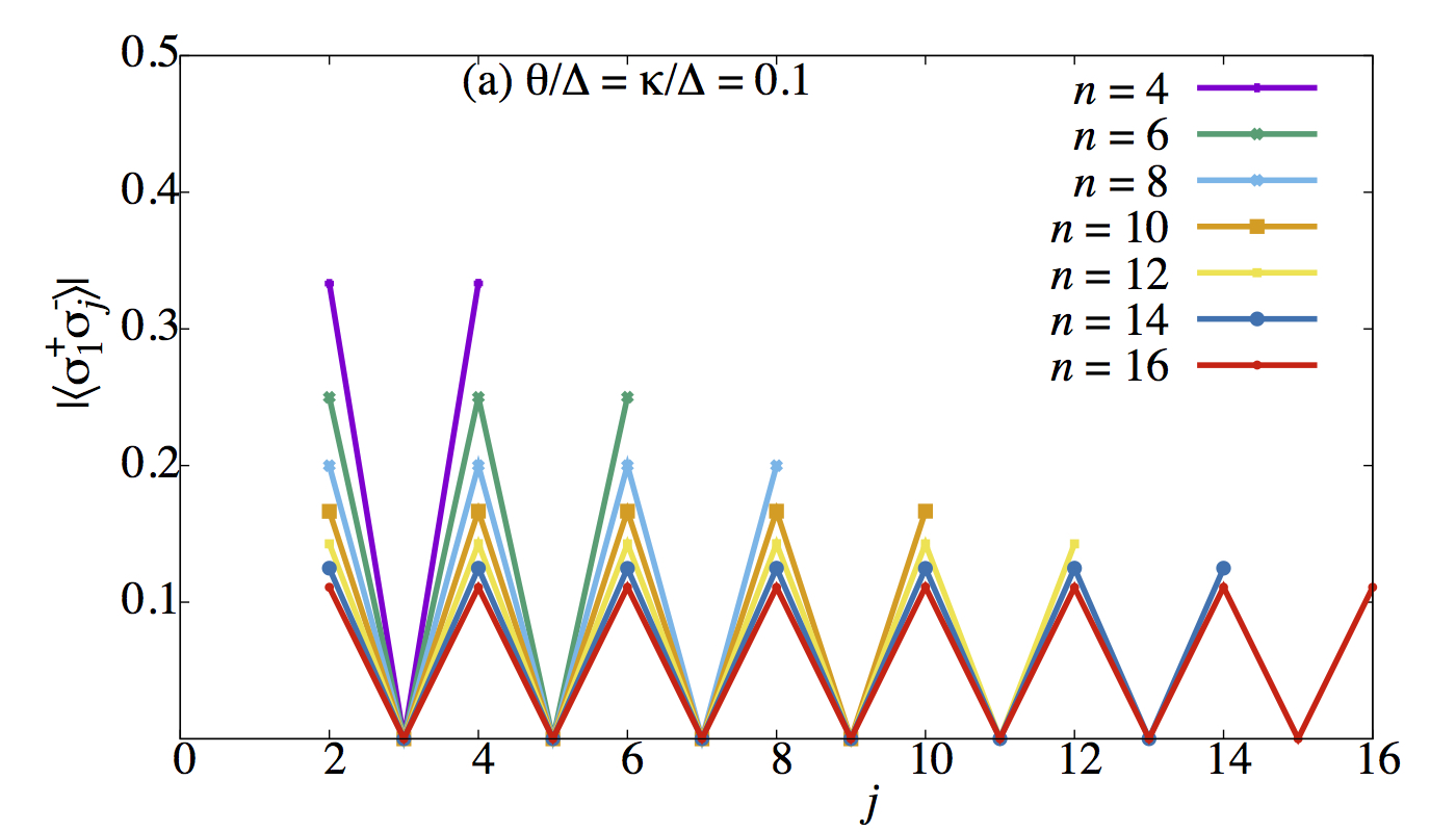
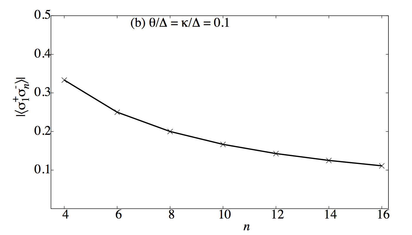
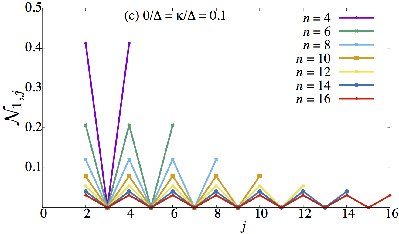
Figure 2: (Color online)(a) Steady state value of the correlator $|\langle\hat{\sigma}_{1}^{+}\hat{\sigma}_{j}^{-}\rangle|$ capturing the pairwise correlations between the first qubit in the primary chain and all other qubits arranged as shown in Fig.1(a). (b) Steady state value of the correlator $|\langle\hat{\sigma}_{1}^{+}\hat{\sigma}_{n}^{-}\rangle|$ capturing the correlations between the 1^st and $n^{\rm th}$ qubits. The numerical results (dot) match perfectly with the analytical result (solid line), confirming linear decay $1/(n/2+1)$ of correlations. (c) Steady state value of the negativity $\mathcal{N}_{1,j}$ capturing the degree of pairwise entanglement between the first qubit in the primary chain and all other qubits arranged in a configuration shown in Fig.1(a).The other dimensionless parameters are $\Delta=1$ and $\Gamma=0.1$.

III.2 Qubit chain: geometry (b)

We now consider another physical scenario of practical interest, where the primary chain is coupled to the two identical secondary chains on its “left” and “right”, as shown in Fig.1(b). The goal is to establish bi-partite correlations between the qubits placed at the remote (open) ends of the two secondary chains. States generated through links joining the qubits located symmetrically with respect to the center (as shown in Fig.1(b)) are also known as rainbow states and have been previously explored in detail in gvit10 ; gram14 . As before, we model the closed dynamics of the qubits in the primary and secondary chains under the following Hamiltonian,

$$\hat{H}_{\rm P-S}^{\rm b}=\hat{H}_{\rm S}^{\rm{L}}+\hat{H}_{\rm P}+\hat{H}_{\rm S}^{R}+\hat{H}_{\rm cplng}^{\rm P-L}+\hat{H}_{\rm cplng}^{\rm P-R},$$ (12)

where $\hat{H}_{\rm P}$ describes the free evolution of the qubits in the primary chain given by equation (2) and,

$$\hat{H}_{\rm S}^{\rm L(R)} = \sum_{j=3,4...}\Delta\hat{\sigma}_{j,\rm{L(R)}}^{z}+\kappa(\hat{\sigma}_{j,\rm{L(R)}}^{+}\hat{\sigma}_{j+1,\rm{L(R)}}^{-}+h.c.),~{}~{}~{}~{}$$

$$\hat{H}_{\rm cplng}^{\rm P-L(R)} = \theta(\hat{\sigma}_{3,\rm{L(R)}}^{+}\hat{\sigma}_{1(2)}^{-}+h.c.).$$

As done in the previous section, we model the open dynamics of the qubits’ arrangement of Fig.1(b) under a master equation of the form,

$$\dot{\hat{\rho}}=-i[\hat{H}_{\rm P-S}^{\rm b},\hat{\rho}]+\Gamma\hat{\mathcal{L}}_{{\hat{b}}_{1,2}}\hat{\rho},$$ (13)

where we have again assumed that the qubits in the primary chain are coupled to an engineered reservoir through the action of the bi-local quantum jump operator ${\hat{b}}_{1,2}$ and the qubits in the secondary chains are assumed to remain noise-free. We assume that the qubits in the primary chain are initially in a state $|\psi(0)\rangle=|\uparrow\rangle_{1}|\downarrow\rangle_{2}$ and the qubits in the left and right secondary chains are initialized in their ground states $|\psi_{j,\rm{L(R)}}(0)\rangle=|\downarrow\rangle_{j,\rm{L(R)}}~{}(j=3,4...)$. We again use the TEBD numerical method for mixed states to time evolve the master equation (13). We find that the time-evolved density matrix $\hat{\rho}(t)$ is a many-body entangled state of the qubits, which exhibit bi-partite quantum correlations across all partitions of the qubits in the primary and secondary chains. However, in contrast to the previous section, numerically obtained $\hat{\rho}(t)$ is a time-dependent mixed state. Furthermore, numerical simulation of the master equation (13) suggests that the time-evolved state $\hat{\rho}(t)$ becomes more mixed as the inter-qubit coupling strengths $\kappa,\theta$ increases.

In order to understand the structure of the time-evolved density matrix $\hat{\rho}(t)$, it is suffice to restrict ourselves to a case when $n$ = 4. Since the master equation (13) conserves the initial number of excitations, the states $|\uparrow\rangle_{3,\rm{L}}|\downarrow\rangle_{1}|\downarrow\rangle_{2}|\downarrow\rangle_{3,\rm{R}};|\downarrow\rangle_{3,\rm{L}}|\uparrow\rangle_{1}|\downarrow\rangle_{2}|\downarrow\rangle_{3,\rm{R}};|\downarrow\rangle_{3,\rm{L}}|\downarrow\rangle_{1}|\uparrow\rangle_{2}|\downarrow\rangle_{3,\rm{R}};|\downarrow\rangle_{3,\rm{L}}|\downarrow\rangle_{1}|\downarrow\rangle_{2}|\uparrow\rangle_{3,\rm{R}}$ form a complete basis set. In this subspace, the Hamiltonian (12) has two eigenstates which are symmetric states of the two primary qubits ($\theta=\kappa$),

$$|\Phi^{\pm}\rangle = \frac{1}{2}(\mp(|\uparrow\rangle_{3,\rm{L}}|\downarrow\rangle_{3,\rm{R}}+|\downarrow\rangle_{3,\rm{L}}|\uparrow\rangle_{3,\rm{R}})|\downarrow\rangle_{1}|\downarrow\rangle_{2}$$

$$+(|\uparrow\rangle_{1}|\downarrow\rangle_{2}+|\downarrow\rangle_{1}|\uparrow\rangle_{2})|\downarrow\rangle_{3,\rm{L}}|\downarrow\rangle_{3,\rm{R}}),$$

with eigenenergies $-(2\Delta\pm\kappa)$. Both the states $|\Phi^{\pm}\rangle$ are dark states of the bi-local Lindblad operator and, therefore, $\hat{\rho}(t)$ is a time-dependent mixture of the states $|\Phi^{\pm}\rangle$. This argument can be easily extended to larger values of $n$ to understand the structure of the time-evolved state $\hat{\rho}(t)$.

In order to stabilize the time-dependent fluctuations in the dynamics of the qubits evolving under the master equation (13), we propose to couple the qubits in the primary chain to two independent dephasing baths. As we will show below, such a counterintuitive arrangement is capable of achieving a time-independent (mixed) entangled steady state of the qubits in the primary and secondary chains. In the presence of additional dephasing baths, the joint dynamics of the qubits in the primary and secondary chains can be modeled as,

$$\dot{\hat{\rho}}=-i[\hat{H}_{\rm P-S}^{\rm b},\hat{\rho}]+\Gamma\hat{\mathcal{L}}_{{\hat{b}}_{1,2}}\hat{\rho}+\gamma\hat{\mathcal{L}}_{{\hat{\sigma}}_{1}^{z}}\hat{\rho}+\gamma\hat{\mathcal{L}}_{{\hat{\sigma}}_{2}^{z}}\hat{\rho}.$$ (14)

We find that a finite but non-zero dephasing rate $\gamma$ can result in a time-independent steady state which is a mixture of bi-partite entangled states. For instance, an exact numerical diagonalization of the master equation (14) for $n=4$ suggests that the steady state is a mixture of entangled states $\hat{\rho}_{1;2}$ and $\hat{\rho}_{3,\rm{L};3,\rm{R}}$. We next use the TEBD method to solve for the steady state of the master equation (14) for different values of $n$. Our numerical simulation of the master equation (14) corroborates in the steady state only the equispaced pair of qubits in the left and right secondary chains have non-zero bi-partite correlations (connected with dashed lines in Fig.1(b)). We evaluate the steady state correlator $|\langle\hat{\sigma}^{+}_{n/2+1,\rm{L}}\hat{\sigma}^{-}_{n/2+1,\rm{R}}\rangle|$ and plot it as a function of $n$ in Fig.3. Our numerical results (dot) confirm that our protocol is capable of generating bi-partite correlations between the qubits placed at the remote (open) ends of the secondary chains. Moreover, the correlator $|\langle\hat{\sigma}^{+}_{n/2+1,\rm{L}}\hat{\sigma}^{-}_{n/2+1,\rm{R}}\rangle|$ decreases linearly ($\sim 1/n$) with the increase in the total number of qubits in the chain (solid line). Fig.3 (b) shows that equispaced pair of qubits in the left and right secondary chains have non-zero degree of bi-partite entanglement $\mathcal{N}_{n/2+1,{\rm L};n/2+1,{\rm R}}$ in the steady state. The resulting impurity of the steady state of the master equation (14) is also reflected in the faster drop of pairwise entanglement shown in Fig.3(b).

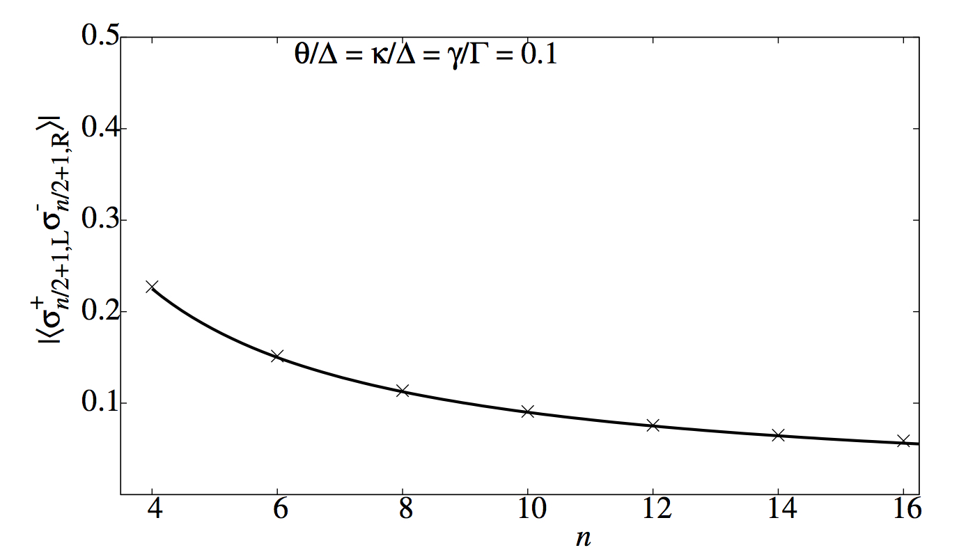
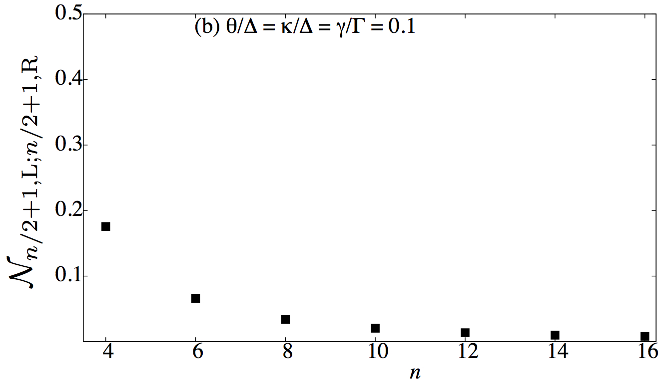
Figure 3: (Color online) (a) The steady state correlator $\langle\hat{\sigma}_{n/2+1,\rm{L}}^{+}\hat{\sigma}_{n/2+1,\rm{R}}^{-}\rangle|$, and (b) the pairwise quantum entanglement $\mathcal{N}_{n/2+1,{\rm L};n/2+1,{\rm R}}$ shown as a function of $n$, capturing the correlations between the qubits placed at the remote (open) ends of the two secondary chains coupled to the two-qubit primary chain, as illustrated in Fig.1(b). The numerical results (dot) confirm a linear drop of correlations $\sim 1/n$ (solid line) in Fig.1(a). The other dimensionless parameters are $\Delta=1$ and $\Gamma=0.1$

IV Outlook and conclusions

In this work, we have presented a protocol for the generation of quantum many-body states of coupled qubits arranged in one-dimensional chains. Our scheme makes use of a reservoir engineering strategy to create a maximally entangled state of the two primary qubits. This quantum state is then transformed to a multi-qubit entangled $W$ state by coherently coupling the primary chain with secondary chains of qubits. Our work allows a possibility to create genuine many-body entangled states which can be useful for short-distance quantum communication protocols sbos03 ; sbos07 ; akay10 ; vngo06 , and also for probing some of the fundamental questions related to the emergence of collective phenomena in many-body open quantum systems sdie08 . Of course, the success of our scheme is critically limited by energy relaxation time of the qubits in the primary and secondary chains. However, it might be possible to use a quantum control technique such as dynamical decoupling strategy to protect the qubits from the unwanted influence of the environment gdel10 ; aber12 ; nbar13 .

One of the natural candidates to testify our method of generation of many-body quantum states will be systems of trapped atomic ions, which exhibit high degree of controllability and manipulability dporr04 ; kkim11 ; rbla12 . Trapped atomic ions also provide a flexibility in generating effective qubit-qubit interactions through external lasers. Moreover, the bi-local quantum jump operator that we have considered has already been implemented in trapped atomic ions jtba11 . If, on the other hand, the qubits in our formalism represent actual spin-1/2 particles then $\Delta$ will be the effective ‘magnetic field’ in the $z$ direction and $\theta,\kappa$ will be the XY coupling strengths between neighboring spins. Our coupled qubits arrangements can also be implemented through chains of coupled quantum dots, where each qubit is represented by the presence or absence of a ground-state exciton. In that case, $\Delta$ will be the exciton energy and $\theta,\kappa$ will be the coupling strengths between neighboring dots. It still remains an open question to address an actual physical implementation of the bi-local quantum jump operator in a physical setting of coupled quantum dots.

There remains an enormous scope for future extensions of our study to explore qubit graphs with more complex geometries sbos07 . In particular, a natural extension of our present work will be to explore in detail the emergence of many-body quantum states in coupled qubits arranged in quasi-one-dimensional configurations, including plaquettes and ladders.

- (1) Steane A. Rep. Prog. Phys. 61, 117 (1998).
- (2) Bennett C. H. and DiVincenzo D. P. Nature 404, 247 (2000).
- (3) Haroche S. Rev. Mod. Phys. 85, 1083 (2013).
- (4) Wineland D. J. Rev. Mod. Phys. 85, 1103 (2013).
- (5) Feynman R. Int. J. Theor. Phys. 21, 467 (1982).
- (6) Porras D. and Cirac J. I. Phys. Rev. Lett. 92, 207901 (2004).
- (7) Kim K. et al. New Journal of Physics 13, 105003 (2011).
- (8) Blatt R. and Roos C. F. Nat. Phys. 8, 277 (2012).
- (9) Georgescu I. M., Ashhab S. and Nori F. Rev. Mod. Phys. 86, 153 (2014).
- (10) Ladd T. D. et al. Nature 464, 45 (2010).
- (11) Zurek W. H. Rev. Mod. Phys. 75, 715 (2003).
- (12) Carvalho A. R. R., Milman P., de Matos Filho R. L. and Davidovich L. Phys. Rev. Lett 86, 4988 (2001).
- (13) Terhal B. M. Rev. Mod. Phys. 87, 307 (2015).
- (14) Sayrin C. et al. Nature 477, 73 (2011).
- (15) Fujii K., Negoro M., Imoto N. and Kitagawa M. Phys. Rev. X 4, 041039 (2014).
- (16) Kelly J. et al. Nature 519, 66 (2015).
- (17) Glaser S. J. et al. Eur. Phys. J. D 69, 279 (2015).
- (18) Y. Liu et al. Phys. Rev. X 6, 011022 (2016).
- (19) Joshi C., Larson J. and Spiller T. Phys. Rev. A 93, 043818 (2016).
- (20) Diehl S. et al. Nat. Phys. 4, 878 (2008).
- (21) Verstraete F., Wolf M. M. and Cirac J. I. Nat. Phys. 5, 633 (2009).
- (22) Krauter H. et al. Phys. Rev. Lett. 107, 080503 (2011).
- (23) Barreiro J. T. et al. Nature 470, 486 (2011).
- (24) Y. Lin et al. Nature 504, 415 (2013).
- (25) Ramos T., Pichler H., Daley A. J. and Zoller P. Phys. Rev. Lett. 113, 237203 (2014).
- (26) Chen C., Yang C.-Jie and An J.-Hong Phys. Rev. A 93, 062122 (2016).
- (27) Poyatos J. F., Cirac J. I. and Zoller P. Phys. Rev. Lett. 77, 4728 (1996).
- (28) Bose S. Phys. Rev. Lett. 91, 207901 (2003).
- (29) Bose S. Contemp. Phys. 48, 13 (2007), and references therein.
- (30) Kay A. Int. J. Quantum Inform. 08, 641 (2010).
- (31) D’Amico I., Lovett B. W. and Spiller T. P. Phys. Rev. A 76, 030302(R) (2007).
- (32) Christandl M., Datta N., Ekert A. and Landahl A. J. Phys. Rev. Lett. 92, 187902 (2004).
- (33) Amico L., Fazio R., Osterloh A. Vedral V. Rev. Mod. Phys. 80, 517 (2008).
- (34) Cubitt T. S. Cirac J. I. Phys. Rev. Lett. 100, 180406 (2008).
- (35) Franco C. D., Paternostro M. and Kim M. S. Phys. Rev. Lett. 101, 230502 (2008).
- (36) Yao N. Y. et al. Phys. Rev. Lett. 106, 040505 (2011).
- (37) Banchi L., Bayat A., Verrucchi P. and Bose S. Phys. Rev. Lett. 106, 140501 (2011).
- (38) Caruso F., Giovannetti V., Lupo C. and Mancini S. Rev. Mod. Phys. 86, 1203 (2014).
- (39) Sahling S. et al. Nat. Phys. 11, 255 (2015).
- (40) Chapman R. J. et al. Nat. Comms. 7, 11339 (2016).
- (41) Breuer H.-P. and Petruccione F. The Theory of Open Quantum Systems, Oxford University Press, Oxford, 2002.
- (42) de Lange G., Wang, Z. H., Riste D., Dobrovitski V. V. and Hanson R. Science 330, 60 (2010).
- (43) Bermudez A., Schmidt P. O.,Plenio M. B. and Retzker A. Phys. Rev. A 85, 040302 (R) (2012).
- (44) Bar-Gill N., Pham L. M., Jarmola A., Budker D. and Walsworth R. L. Nat. Commun 4, 1743 (2013).
- (45) Zwolak M. and Vidal G. Phys. Rev. Lett. 93, 207205 (2004).
- (46) See Joshi C., Nissen F. and Keeling J. Phys. Rev. A 88, 063835 (2013), and references therein.
- (47) Dür W., Vidal G. and Cirac J. I.Phys. Rev. A 62, 062314 (2000).
- (48) Gorbachev V. N. and Trubilko A. I. Laser Phys. Lett. 3, 59 (2006).
- (49) Nielsen M. A. and Chuang I. L. Quantum Computation and Quantum Information, Cambridge University Press, Cambridge, 2010.
- (50) Häffner H. et al. Nature 438,, 643 (2005).
- (51) Matthew N. et al. Nature 467, 570 (2010).
- (52) Reiter F., Reeb D. and Sørensen A. S., arXiv:1501.06611.
- (53) Aron C., Kulkarni M. and Türeci H. E. Phys. Rev. X 6, 011032 (2016).
- (54) Kiffner M. and Hartmann M. J. New Journal of Physics 13, 053027 (2011).
- (55) Vitagliano G. and Latorre J. I.New Journal of Physics 12, 113049 (2010).
- (56) Ramírez G., Rodr guez-Laguna J. and Sierra G.J. Stat. Mech. P10004 (2014).