From the density-of-states method to finite density quantum field theory

Abstract

During the last 40 years, Monte Carlo calculations based upon Importance Sampling have matured into the most widely employed method for determinig first principle results in QCD. Nevertheless, Importance Sampling leads to spectacular failures in situations in which certain rare configurations play a non-secondary role as it is the case for Yang-Mills theories near a first order phase transition or quantum field theories at finite matter density when studied with the re-weighting method. The density-of-states method in its LLR formulation has the potential to solve such overlap or sign problems by means of an exponential error suppression. We here introduce the LLR approach and its generalisation to complex action systems. Applications include U(1), SU(2) and SU(3) gauge theories as well as the Z3 spin model at finite densities and heavy-dense QCD.

11.15.Ha 12.38.Aw 12.38.Gc

1 Introduction

Recently, Monte Carlo sampling methods for determining density-of-states have seen a surge of interest. An integral part of these novel density-of-state methods is a re-weighting with the inverse density-of-states providing feedback for an iterative refinement of this quantity [1]. Deriving the density-of-states in this way, within chosen action intervals, allows us to obtain this observable for regions of actions that conventional Importance Sampling algorithms would never visit in practical simulation times. For this reason, the density-of-state approach solves overlap problems, which manifest when large tunnelling times, generally growing exponentially with the size of the system, separate regions of equally important statistical weight, henceforth causing an asymptotic ergodicity problem in the latter algorithms. Methods based on iterative refinements of the density-of-states fall into the class of non-Markovian Random Walks. They extend outside the domain of Importance Sampling the observation that a random walk in configuration space is not plagued by exponentially large tunnelling times [2]. In this paper, we focus on the Linear Logarithmic Relaxation (LLR) algorithm [3], which is particularly suited for theories with continuous degrees of freedom, and in particular for gauge theories. We here summarise the foundations of the LLR method and its applications to gauge theories (see [4] and [5]) and then focus on recent successes of the LLR approach to quantum field theories at finite densities [6, 7].

2 The density-of-states approach

2.1 The Logarithmic Linear Relaxation (LLR) algorithm

Our starting point is the partition function of an Euclidean quantum field theory

$$Z(\beta)=\int{\cal D}\phi\;\e^{\beta S[\phi]}\;.$$

The density-of-states $\rho(E)$ quantifies the amount of states if the configurations are constrained to the action hyper-plane $E=S[\phi]$. Its precise definition and relation to the partition function are:

$$\rho(E)=\int{\cal D}\phi\;\delta\Bigl{(}S[\phi]-E\Bigr{)}\;,\hbox to28.45274pt{\hfill}Z(\beta)=\int dE\;\rho(E)\;\e^{\beta E}\;.$$ (1)

Our goal will be to obtain $\rho(E)$ with very high precision and to directly calculate the partition function $Z$ by performing the integral over $E$ [3]. To this aim, we divide the action range into intervals of size $\delta E$. If the action interval is small enough, we can approximate the density-of-states by a Poisson-like distribution:

$$\rho(E)\propto\e^{\alpha E}\,,\hbox to28.45274pt{\hfil for \hfil}E_{k}-\frac{\delta E}{2}\leq E\leq E_{k}+\frac{\delta E}{2},\hbox to28.45274pt{\hfill}\alpha_{k}=\frac{d\ln\,\rho}{dE}\Big{|}_{E=E_{k}}.$$

Our strategy is to calculate the LLR coefficients $\alpha_{k}$ and to reconstruct $\rho(E)$. To this aim, we define the “double-bracket” Monte-Carlo expectation value with $a$ being an external parameter:

$$\left\langle\kern-1.69998pt\left\langle W[\phi]\right\rangle\kern-1.69998pt\right\rangle_{k}(a) = \frac{1}{{\cal N}_{k}}\int{\cal D}\phi\;\theta_{[E_{k},\delta E]}(S[\phi])\;W[\phi]\;\,\e^{-aS[\phi]}\;,$$ (2)

$${\cal N}_{k} = \int{\cal D}\phi\;\theta_{[E_{k},\delta E]}\;\,\e^{-aS[\phi]}\;,$$ (3)

where we have introduced the modified Heaviside function

$$\theta_{[E_{k},\delta E]}(S)\;=\;\left\{\begin{array}[]{ll}1&\hbox{for}\;\;\;E_{k}-\delta E/2\leq S\leq E_{k}+\delta E/2\\ 0&\hbox{otherwise . }\end{array}\right.$$

The key observation is that for $a=\alpha_{k}$, the probability distribution for $\phi$ over the action interval becomes flat since the re-weighting factor $\exp\{-aS\}$ compensates the density-of-states $\exp\{\alpha_{k}S\}$. Choosing $W[\phi]=S[\phi]-E_{k}$ as Litmus paper for flatness, we observe:

$$\left\langle\kern-1.69998pt\left\langle S[\phi]-E_{k}\right\rangle\kern-1.69998pt\right\rangle_{k}(a)\;=\;0\hbox to56.9055pt{\hfil for \hfil}a\;=\;\alpha_{k}\;=\;\frac{d\ln\,\rho}{dE}\Big{|}_{E=E_{k}}.$$ (4)

This equation is at the heart of the LLR approach: it allows to calculate the log-derivative $\alpha_{k}$ of the log derivative of $\rho$ by solving the stochastic non-linear equation $\left\langle\kern-1.69998pt\left\langle S[\phi]-E_{k}\right\rangle\kern-1.69998pt\right\rangle_{k}(a)\;=\;0$ for $a$. We stress that the expectation values $\left\langle\kern-1.69998pt\left\langle\ldots\right\rangle\kern-1.69998pt\right\rangle$ are accessible by standard Monte-Carlo simulations.

A simple procedure to find the root of a function is the iterative Newton-Raphson method

$$a_{n+1}=a_{n}+\frac{\left\langle\kern-1.69998pt\left\langle S[\phi]-E_{k}\right\rangle\kern-1.69998pt\right\rangle_{k}(a_{n})}{\left\langle\kern-1.69998pt\left\langle(S-E_{k})^{2}\right\rangle\kern-1.69998pt\right\rangle_{k}}\approx a_{n}+\frac{12}{\delta E^{2}}\,\left\langle\kern-1.69998pt\left\langle S[\phi]-E_{k}\right\rangle\kern-1.69998pt\right\rangle_{k}(a_{n})\;.$$

Note, however, that the statistical error from the Monte-Carlo estimate for $\left\langle\kern-1.69998pt\left\langle S[\phi]-E_{k}\right\rangle\kern-1.69998pt\right\rangle_{k}$ interferes with the convergence of the Newton iteration. The solution to the root-finding procedure for stochastic equations has been found by Robinson and Monro. The iterative Robinson-Monro algorithm has the form

$$a_{n+1}=a_{n}-c_{n}\;\left\langle\kern-1.69998pt\left\langle S[\phi]-E_{k}\right\rangle\kern-1.69998pt\right\rangle_{k}(a_{n}),\qquad\mathrm{with}\ \sum_{n=0}^{\infty}c_{n}=\infty\ \mathrm{and}\ \sum_{n=0}^{\infty}c_{n}^{2}<\infty$$

Robinson-Monro proved that $\lim_{n\to\infty}a_{n}=\alpha_{k}$ with $a_{n}$ asymptotically normally distributed around $\alpha_{k}$. To minimise the variance of the result one chooses

$$c_{n}=\frac{12}{\delta E^{2}\,(n+1)}\;.$$

Once the LLR coefficients $a_{k}$ are obtained for the action range, the density-of-states can be obtained by

$$\rho(E)=\prod_{i=1}^{k-1}e^{{a}(E_{i})\frac{\delta E}{2}}\exp\Bigl{(}a(E_{k})(E-E_{k})\Bigr{)}\,,\qquad E_{k}\leq E<E_{k+1}\;.$$ (5)

The LLR method has some remarkable features [4]:

• Almost everywhere, we find that the LLR approximated result $\rho(E)$ (5) is related to the exact density-of-states by

  $$\rho(E)\;\e^{\gamma_{1}\,\delta E^{2}}\;\leq\;\rho_{\mathrm{exact}}(E)\;\leq\;\rho(E)\;\e^{\gamma_{2}\,\delta E^{2}}\ ,\ \gamma_{1},\ \gamma_{2}\ \mathrm{constants}.$$

  The approach has exponential error suppression: the relative approximation error does not depend on the magnitude of $\rho$ despite $\rho$ might span thousands of orders of magnitude.

• The LLR approach can be generalised to calculate expectation value of arbitrary observables (rather than the partition function only). The systematic error is ${\cal O}(\delta E^{2})$. See [4] for details.

2.2 The generalised density-of-states

Quantum Field Theories at finite matter densities (or more precisely, at non-vanishing chemical potential $\mu$) are generically plagued by the so-called sign problem. In this case, the partition function, which features a complex action, can be written in the general form as

$$Z(\beta,\mu)=\int{\cal D}\phi\;\exp\Bigl{\{}\beta\,S_{R}[\phi]+i\,\mu\,S_{I}[\phi]\Bigr{\}}\;.$$ (6)

The Gibbs factor looses the interpretation as probability density and Importance Sampling is impossible. An early attempt to circumvent the sign problem was to drop the phase factor when generating the lattice configuration and to add the phase factor to the observable:

$$\langle A\rangle\;=\;\frac{\langle A\,\exp\{i\,\mu\,S_{I}[\phi]\}\rangle_{\mathrm{PQ}}}{\langle\exp\{i\,\mu\,S_{I}[\phi]\}\rangle_{\mathrm{PQ}}}\;,\hbox to28.45274pt{\hfill}Z_{\mathrm{PQ}}\;=\;\int{\cal D}\phi\;\exp\Bigl{\{}-\beta\,S_{R}[\phi]\Bigr{\}}\;.$$

In this phase quenched approach, we encounter an overlap problem. Following [6, 5], we define the overlap between full and phase quenched theory by the ratio of their partition functions, i.e.,

$$Q(\mu)\;=\;\frac{Z(\mu)}{Z_{\mathrm{PQ}}(\mu)}\;=\;\left\langle\exp\{i\,\mu\,S_{I}[\phi]\}\right\rangle_{\mathrm{PQ}}\;.$$ (7)

Since the phase-quenched theory has a positive probabilistic measure, we find by virtue of the triangular inequality that [5]

$$|Q(\mu)|\leq\Bigl{\langle}|\exp\{i\,\mu\,S_{I}[\phi]\}|\Bigr{\rangle}_{\mathrm{PQ}}\;=\;1\;.$$

Note, however, that both theories generically differ in their free energies $f$, leading to exceptionally small overlaps at large volumes $V$:

$$Q(\mu)\;=\;\exp\Bigl{\{}-\,\Delta f\;V\Bigr{\}}\;,\hbox to28.45274pt{\hfill}\Delta f\geq 0\;.$$

Since the LLR method generically solves overlap problems, we extend the approach outlined in the previous subsection and define the generalised density-of-states by

$$\rho_{\beta}(s)\;=\;N\;\int{\cal D}\phi\;\delta\Bigl{(}s\,-\,S_{I}[\phi](\mu)\,\Bigr{)}\;\e^{\beta\,S_{R}[\phi](\mu)}\;,$$ (8)

with $N$ an unknown normalisation factor independent of $s$. The overlap then appears as the Fourier transform of the generalised density:

$$Q(\mu)\;=\;\frac{\int ds\;\rho_{\beta}(s)\;\exp(is)}{\;\int ds\;\rho_{\beta}(s)}\;.$$

Note that the unknown normalisation $N$ has dropped out.

3 Vacuum applications: U(1), SU(2) SU(3) Yang-Mills theories

 

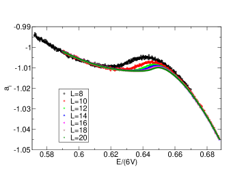
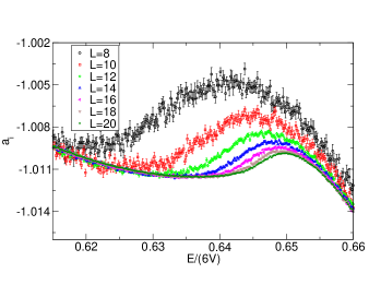
Figure 1: LLR coefficient $a(E)$ (or $\alpha(E)=d\,\ln\rho/dE$) as a function of the action $E$ for a U(1) gauge theory for several lattice volumes.

In the following, we show the LLR method in action for pure gauge theories in vacuum, i.e., without finite density matter and no-sign problem. The degrees of freedom are the link fields $U_{\mu}(x)\in$U(1), SU(2) or SU(3), and the action is given by

$$S\;=\;\sum_{\nu>\mu,x}\frac{1}{N_{c}}\,\mathrm{Re}\,\hbox{tr}\{U_{\mu}(x)U_{\nu}(x+\mu)U^{\dagger}_{\mu}(x+\nu)U^{\dagger}_{\nu}(x)\,\}\;,$$

where $N_{c}$ is the number of colours ($N_{c}=1$ for U(1)), the ’Re’ can be omitted for SU(2), since the theory is real, and the trace ’tr’ is absent for U(1). The empty (perturbative) vacuum is attained with $S=6V$ where $V$ is the volume, i.e., the number of lattice points.

 

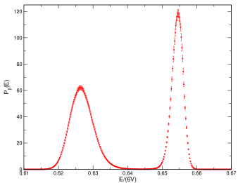
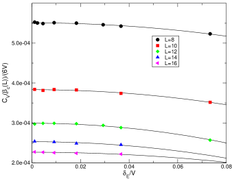
Figure 2: Left: Probability distribution of the action for a U(1) gauge theory on a $20^{4}$ lattice at criticality. Right: Specific heat as function of the interval discretisation length $\delta E$ (results from [4]).

For each of these theories, the probabilistic measure rises from the product of the density-of-states and the Gibbs factor:

$$P(E)\;=\;\rho(E)\,\exp\{\beta E\}\;.$$ (9)

 

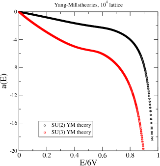
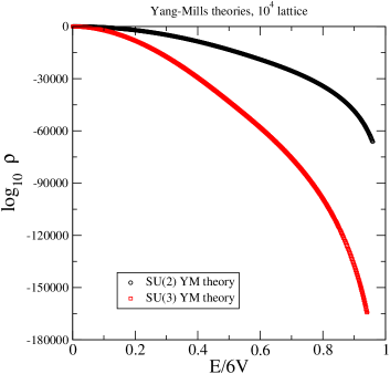
Figure 3: Left: The LLR coefficient $a(E)$ as a function of the action $E$ on a $10^{4}$ lattice for a SU(2) and SU(3) Yang-Mills theory. Right: The corresponding density-of-states. Results from [5].

Generically, $\rho(E)$ monotonically decreases with $E$ while the Gibbs factor exponentially increases. Thus, $P(E)$ settles for a sharp maximum (away from first order criticality). The most likely value for the action can be calculated from:

$$\frac{dP(E)}{dE}\;=\;\rho(E)\,\exp\{\beta E\}\Bigl{[}\alpha(E)\;+\;\beta\Bigr{]}\;=\;0\;$$ (10)

Away from criticality, this equation most have just one solution for each $\beta$. This observation can be used to calculate $\rho(E)$ for small $E$ using the strong coupling expansion [5]. For a first order phase transition at $\beta=\beta_{c}$, $P(E)$ exhibits the typical double-peak structure. Hence, $P(E)$ features two maxima and one minimum meaning that (10) has three solutions. Let us illustrate this for the U(1) gauge theory [4], for which our findings for the LLR coefficient are shown in figure 1. In accordance with the theory [4], $a(E)$ becomes volume independent at large volumes. In the region between $E/6V=0.61$ and $E/6V=0.66$, we observe a non-monotonic behaviour that leads to three solutions of the equation (10) for a suitably chosen $\beta$. Our result for $P(E)$ for a lattice as large as $20^{4}$ is shown in figure 2. We stress that our result is obtained for an un-rivalled lattice and that we do not see a significant critical slowing-down while increasing the lattice size. A more detailed analysis of the volume scaling properties of our algorithm is left to future work. Using the specific heat $C_{v}$, we also studied the systematic errors induced by the finite action interval size $\delta E$. Figure 2 shows $C_{V}$ as a function of $\delta E$ for several values $\delta E$. Our numerical results suggest a quadratic behaviour in $\delta E$, which is in accordance with the theory [4].

We finally show the results for the SU(2) and SU(3) Yang-Mills theory on a $10^{4}$ lattice. Figure 3 shows $a(E)=d\,\ln\rho/dE$ as a function of the action $E$. Also shown is the leading order analytical result at small $E$ [5]. In the same figure, we also show the reconstructed density-of-states (5). The error bars were obtained by a bootstrap analysis of $40$ independent results for $a(E)$ for each $E$. Note the logarithmic vertical axis: for SU(3), we obtain the density-of-states over $150,000$ orders of magnitude with an almost constant statistical error bar over the whole action range.

4 Applications to finite density quantum field theories

4.1 The $Z_{3}$ theory as showcase

 

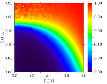
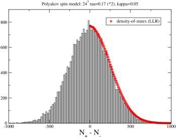
Figure 4: Left: Phase diagram of the $Z_{3}$ theory as function of the chemical potential $\mu$ and $\tau$ (say temperature). Right: The probability distribution of the imaginary part of the action.

 

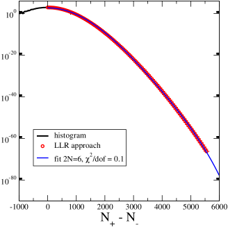
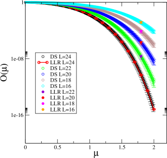
Figure 5: Left: Same as figure 4, right panel, on a logarithmic scale (result from [5]). Right: LLR-result for the overlap factor $Q(\mu)$ as function of $\mu$ (result from [6]).

The $Z_{3}$ theory in three dimensions is inspired by QCD if the $Z_{3}$ degrees of freedom on site are identified with the Polyakov line. The partition function as well as the action of the system are given by

$$Z(\mu) = \sum_{\{\phi\}}\;\exp\Bigl{(}S[\phi]\Bigr{)}\;,\;\;\;S[\phi]=\tau\sum_{x,\nu}\phi_{x}\,\phi^{\ast}_{x+\nu}+\sum_{x}\,\Bigl{(}\eta\phi_{x}+\bar{\eta}\phi^{\ast}_{x}\Bigr{)}\;,$$ (11)

with $\eta=\kappa\,\mathrm{e}^{\mu}$ and $\bar{\eta}=\kappa\,\mathrm{e}^{-\mu}$. For non-vanishing chemical potential, we have $\eta\not=\bar{\eta}^{\ast}$ and the theory has a sign problem. Note, however, that this theory has a real dual formulation [8, 9, 10], and can be efficiently simulated with the flux algorithm[11]. The phase diagram can be readily calculated (see figure 4, left panel for our result) and bears a certain similarity of what we expect for the QCD phase diagram. Here, it serves as an ideal benchmark for testing the generalised LLR approach [6].

The probability distribution of the imaginary part $\rho_{\beta}(s)$ (see (8)) can be obtained by generating lattice configurations with respect to the phase quenched theory and by subjecting the imaginary part to a histogram. The result is shown in the right panel of figure 4. Alternatively, we can calculate $\rho_{\beta}(s)$ using the LLR formalism. The result is also shown in figure 4: a good agreement of the LLR result with the histogram is observed. We point out that the histogram method fails to produce an accurate estimate for $\rho_{\beta}(s)$ at large imaginary parts since hardly any events are recorded in this case. This is a manifestation of the overlap problem. The LLR method solves this overlap problem, and, by virtue of the exponential error suppression, produces very good results over many orders of magnitude (see figure 5, left panel).

In order to obtain the overlap $Q(\mu)$, a Fourier transform of the probability distribution $\rho_{\beta}(s)$ must be carried out. Since the overlap exponentially decreases with the volume, the result of the Fourier transform will generically produce a very small signal. Despite of the precision for $\rho_{\beta}(s)$ that can be reached with the LLR method, compressing the numerical data into an analytic model with few parameters has proven essential [5]:

$$\ln\rho(n)=\lim_{N\to\infty}\sum_{k=1}^{N}c_{k}\;f_{k}(n)\;,$$ (12)

where $f_{k}(n)$ are basis functions. The approximation arises from the truncation of the above sum. For the $Z_{3}$ spin system, good results are obtained by using powers of $n$: $f_{k}(n)=n^{2k}$. Here we have exploited the symmetry $\rho(-n)=\rho(n)$, which eliminates odd powers of $n$ from the basis. Figure 5, left panel, shows a typical result for such a fit. We find that for $N$ bigger than some threshold $N_{th}$, the fits stabilise: the fit results agree within error bars for $N\geq N_{th}$. Usually, the error bars tend to increase for larger values of $N$. Hence, we use the fit result for $N=N_{th}$ (and the corresponding statistical error bars from the bootstrap analysis). Figure 5, right panel, compares the LLR result with the results from a simulation of the dual (real) theory. We find an excellent agreement despite of the fact that the overlap becomes as small as $10^{-16}$ for the largest lattice size.

4.2 QCD at finite densities of heavy quarks

 

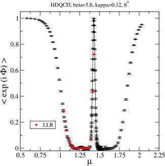
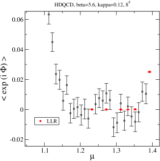
Figure 6: Left: The overlap factor for HDQCD as a function of the quark chemical potential (result from [7]). Right: Detail of left panel.

 

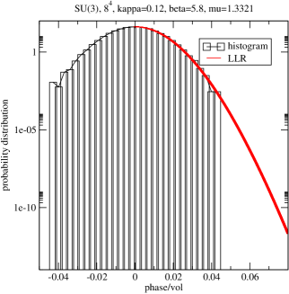
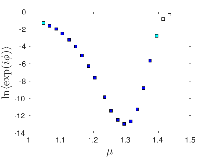
Figure 7: Left: Probability distribution of the imaginary part of the quark determinant. Right: LLR result for the log of the overlap factor (results from [7]).

Our starting point is the QCD partition function

$$Z(\mu)\;=\;\int{\cal D}U_{\mu}\;\exp\{\beta\,S_{\mathrm{YM}}[U]\}\;\hbox{Det}M(\mu)\;,$$ (13)

from which the quarks have been integrated out leaving us with the quark determinant. In the so-called heavy-dense limit for large quark mass $m$ and simultaneously large chemical potential $\mu$, the quark determinant factorises into [12, 13, 14, 15, 16]:

$$\hbox{Det}\,M(\mu) = \prod_{\vec{x}}\;{\det}^{2}\Bigl{(}1\,+\,\,\e^{(\mu-m)/T}\,P(\vec{x})\Bigr{)}{\det}^{2}\Bigl{(}1\,+\,h\,\e^{-(\mu+m)/T}\,P^{\dagger}(\vec{x})\Bigr{)}\;,$$

where $m$ is the mass of the heavy quark, $T=1/N_{t}a$ is the temperature with $a$ the lattice spacing and $N_{t}$ the number of lattice points in the temporal direction. At small temperatures $T\ll m$, we can ignore the latter determinant in the latter equation. The theory is then not only real at vanishing chemical potential, but also at threshold $\mu=m$ (also called “half-filling”) and the theory exhibits a particle-hole duality [16, 7]. Adopting a standard re-weighting approach, we find for the overlap factor the result shown in figure 6. At intermediate values for the chemical potential, we do encounter a strong sign problem: the re-weighting method produces results that are within statistical errors compatible with zero implying that we have lost the signal in the noise.

To tackle this problem, we again employed the LLR approach to get high quality results for the probability distribution of the phase of the quark determinant. We checked that our results agree with those from a straightforward histogram method (see figure 7). Based upon our experience with the $Z_{3}$ theory, we adopted the same method to obtain the density’s Fourier transform (see (12) and discussions below). Our final result for the overlap nicely agrees in regions of the chemical potential where re-weighting can produce statistical significant results (see figure 6). Note, however, that the LLR result has error bars that are five orders of magnitude smaller. Our final high quality result for the overlap is shown in figure 7, left panel, and we refer the reader to [7] for further discussions.

Acknowledgements: We thank N. Garron, A. Rago and R.  Pellegrini for helpful discussions. We are grateful to the HPCC Plymouth and HPC Wales for support received for carrying out numerical simulations. KL is supported by the Leverhulme Trust (grant RPG-2014-118) and by STFC (grant ST/L000350/1). BL is supported by STFC (grant ST/L000369/1).

References

- Wang and Landau [2001] Fugao Wang and D. P. Landau. Efficient, multiple-range random walk algorithm to calculate the density of states. Phys. Rev. Lett., 86(10):2050–2053, Mar 2001. 10.1103/PhysRevLett.86.2050.
- Berg and Neuhaus [1992] B. A. Berg and T. Neuhaus. Multicanonical ensemble: A New approach to simulate first order phase transitions. Phys. Rev. Lett., 68:9–12, 1992. 10.1103/PhysRevLett.68.9.
- Langfeld et al. [2012] Kurt Langfeld, Biagio Lucini, and Antonio Rago. The density of states in gauge theories. Phys. Rev. Lett., 109:111601, 2012. 10.1103/PhysRevLett.109.111601.
- Langfeld et al. [2016] Kurt Langfeld, Biagio Lucini, Roberto Pellegrini, and Antonio Rago. An efficient algorithm for numerical computations of continuous densities of states. Eur. Phys. J., C76(6):306, 2016. 10.1140/epjc/s10052-016-4142-5.
- Gattringer and Langfeld [2016] Christof Gattringer and Kurt Langfeld. Approaches to the sign problem in lattice field theory. 2016.
- Langfeld and Lucini [2014] Kurt Langfeld and Biagio Lucini. Density of states approach to dense quantum systems. Phys. Rev., D90(9):094502, 2014. 10.1103/PhysRevD.90.094502.
- Garron and Langfeld [2016] Nicolas Garron and Kurt Langfeld. Anatomy of the sign-problem in heavy-dense QCD. 2016.
- DeGrand and DeTar [1983] Thomas A. DeGrand and Carleton E. DeTar. Phase Structure of QCD at High Temperature With Massive Quarks and Finite Quark Density: A (3) Paradigm. Nucl.Phys., B225:590, 1983.
- Patel [1984] Apoorva Patel. A Flux Tube Model of the Finite Temperature Deconfining Transition in QCD. Nucl.Phys., B243:411, 1984.
- Mercado et al. [2011] Ydalia Delgado Mercado, Hans Gerd Evertz, and Christof Gattringer. The QCD phase diagram according to the center group. Phys.Rev.Lett., 106:222001, 2011.
- Mercado et al. [2012] Ydalia Delgado Mercado, Hans Gerd Evertz, and Christof Gattringer. Worm algorithms for the 3-state Potts model with magnetic field and chemical potential. Comp. Phys. Com., 183:1920–1927, 2012.
- Bender et al. [1992] I. Bender, T. Hashimoto, F. Karsch, V. Linke, A. Nakamura, M. Plewnia, I. O. Stamatescu, and W. Wetzel. Full QCD and QED at finite temperature and chemical potential. Nucl. Phys. Proc. Suppl., 26:323–325, 1992. 10.1016/0920-5632(92)90265-T.
- Blum et al. [1996] Thomas C. Blum, James E. Hetrick, and Doug Toussaint. High density QCD with static quarks. Phys. Rev. Lett., 76:1019–1022, 1996. 10.1103/PhysRevLett.76.1019.
- Aarts et al. [2014] Gert Aarts, Felipe Attanasio, Benjamin Jager, Erhard Seiler, Denes Sexty, and Ion-Olimpiu Stamatescu. QCD at nonzero chemical potential: recent progress on the lattice. In 11th Conference on Quark Confinement and the Hadron Spectrum (Confinement XI) St. Petersburg, Russia, September 8-12, 2014, 2014.
- Aarts et al. [2015] Gert Aarts, Felipe Attanasio, Benjamin Jäger, Erhard Seiler, Dénes Sexty, and Ion-Olimpiu Stamatescu. The phase diagram of heavy dense QCD with complex Langevin simulations. Acta Phys. Polon. Supp., 8(2):405, 2015. 10.5506/APhysPolBSupp.8.405.
- Rindlisbacher and de Forcrand [2016] Tobias Rindlisbacher and Philippe de Forcrand. Two-flavor lattice QCD with a finite density of heavy quarks: heavy-dense limit and “particle-hole” symmetry. JHEP, 02:051, 2016. 10.1007/JHEP02(2016)051.