Device-independent dimension tests in the prepare-and-measure scenario

Abstract

Analyzing the dimension of an unknown quantum system in a device-independent manner, i.e., using only the measurement statistics, is a fundamental task in quantum physics and quantum information theory. In this paper, we consider this problem in the prepare-and-measure scenario. Specifically, we provide a lower bound on the dimension of the prepared quantum systems which is a function that only depends on the measurement statistics. Furthermore, we show that our bound performs well on several examples. In particular, we show that our bound provides new insights into the notion of dimension witness, and we also use it to show that the sets of restricted-dimensional prepare-and-measure correlations are not always convex.

In the device-independent paradigm one tries to understand the properties of an unknown (classical or quantum) system based only on the correlations resulting from measurements performed on the system BPA+08 ; WCD08 ; VSW15 ; BCP14 ; GBHA10 ; BQB14 ; HGM+12 ; ABCB12 ; LBL+15 ; BNV13 ; CBRS16 ; GBS16 ; CKKS16 ; CBB15 . In this work we consider the problem of lower bounding the dimension of a uncharacterized quantum system in a device-independent manner. This problem is quite interesting from the viewpoints of both physics and quantum computation, and has attracted much attention BPA+08 ; WCD08 ; VSW15 ; BCP14 ; GBHA10 ; BQB14 ; HGM+12 ; ABCB12 ; BNV13 ; CBRS16 . Indeed, the dimension of a quantum system is a fundamental physical property, and is also widely regarded as a valuable computational resource, as one always tries to implement an algorithm or protocol with the smallest dimension possible.

This question was first considered in the Bell scenario BPA+08 ; WCD08 ; VSW15 ; BCP14 where a quantum system is shared by two parties, each performing local measurements on their own subsystems, illustrated in FIG. 1(a). The corresponding set of measurement statistics is called a Bell correlation. Then the task is, for a given Bell correlation, to lower bound the dimension of the underlying quantum system. In BPA+08 , the dimension witness approach was introduced to address this problem. A (linear) $d$-dimensional witness is defined as a hyperplane that contains all Bell correlations that can be generated using $d$-dimensional quantum systems in one of its halfspaces. However, though providing very strong and intuitive physical insights, dimension witnesses can suffer from two apparent drawbacks. First, dimension witnesses do not always give a lower bound on the dimension of the underlying quantum system as a direct function of the correlation data. Second, identifying dimension witnesses amounts to characterizing the complicated structure of quantum correlations with restricted dimensions, which is often a very challenging task.

Another approach was recently introduced in an attempt to overcome these difficulties. Specifically, a new lower bound on the dimension of a quantum system needed to generate a Bell correlation was given in VSW15 . This bound is easy to calculate as it is a simple function of the Bell correlation and is tight in many cases.

The dimension witness approach was later generalized to the prepare-and-measure (PM) scenario which is simpler and more general GBHA10 . Unlike the Bell scenario, the PM scenario does not involve entanglement, and this makes it easier to implement experimentally HGM+12 ; ABCB12 ; LBL+15 . In the PM scenario, one party, the preparer, prepares one of finitely many quantum states, then the other party, the measurer, performs one of finitely many measurements on the state, see FIG. 1(b). The corresponding set of measurement statistics is called a PM correlation. Similar to the Bell scenario, a very important and natural problem is to lower bound the dimension of the quantum system required to generate a given PM correlation. For this, the approach of linear dimension witness was generalized to the PM scenario in GBHA10 , where the preparer and the measurer share classical public randomness. The case where the devices are independent was considered in BQB14 , where one needs to use nonlinear dimension witnesses.

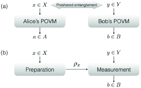
Figure 1: (a) A Bell scenario. (b) A prepare-and-measure scenario.

Despite these encouraging results, dimension witnesses in the PM scenario suffer from similar drawbacks as those for the Bell scenario, which restricts their applicability. Indeed, some are very specific, e.g., the dimension witnesses discussed in GBHA10 ; BQB14 apply only for the case of binary measurements. Consequently, it is highly desirable to identify a lower bound for the PM scenario, analogous to that in VSW15 , that is applicable to PM correlations with arbitrary parameters. In this work, we provide such a new lower bound. To achieve this, we first transfer the target PM scenario to a corresponding Bell scenario, and then apply the bound given in VSW15 , leading to a new lower bound for PM correlations. We show that the new lower bound performs very well on some interesting applications, e.g. quantum random access coding, and it also gives new insights for the concept of dimension witness. Specifically, we show that the dimension witness provided in BNV13 can be obtained as a direct consequence of our new lower bound. Furthermore, we also use our lower bound to prove that the sets of restricted-dimensional PM correlations are not always convex.

Scenarios. A two-party Bell scenario consists of two parties, Alice and Bob, that are in separate locations, and share a quantum state $\rho$ acting on $\mathbb{C}^{d_{1}}\otimes\mathbb{C}^{d_{2}}$. Alice and Bob each have a (local) measurement apparatus acting on their respective subsystems, see FIG. 1(a). A Bell correlation $r$ is the collection of the joint conditional probabilities $r(a,b|x,y)$, i.e., the probability Alice and Bob get output $(a,b)\in A\times B$ when they use measurement settings $(x,y)\in X\times Y$. In VSW15 , it was shown that for a given Bell correlation $r=r(a,b|x,y)$, both $d_{1}$ and $d_{2}$ are lower bounded by the following two quantities:

$$\!\!\!\!\max_{y,y^{\prime}}\Big{(}\displaystyle\sum_{b,b^{\prime}}\min_{x}\Big{(}\sum_{a}\sqrt{r(a,b|x,y)}\sqrt{r(a,b^{\prime}|x,y^{\prime})}\Big{)}^{2}\Big{)}^{-1},$$ (1)

$$\!\!\!\!\max_{x,x^{\prime}}\Big{(}\displaystyle\sum_{a,a^{\prime}}\min_{y}\Big{(}\sum_{b}\sqrt{r(a,b|x,y)}\sqrt{r(a^{\prime},b|x^{\prime},y)}\Big{)}^{2}\Big{)}^{-1}.$$ (2)

As mentioned above, a PM scenario has one party preparing a quantum state and the other measuring it, thus the outcome probabilities are only seen on one side. The preparer can generate one out of $N$ possible states, denoted by $\rho_{x}$, where $x\in X=\{1,2,...,N\}$. The measurer can choose one of $M$ different measurements to perform, indexed by $y\in Y=\{1,\ldots,M\}$. Each measurement $y$ consists of the operators $\{\Pi_{b}^{y}\}$, where $b\in B=\{1,\ldots,K\}$ denotes the measurement outcome. The probability of getting outcome $b$ when measurement $y$ is performed on quantum state $\rho_{x}$ can thus be expressed as $p(b|x,y)=\mathrm{Tr}(\rho_{x}\Pi_{b}^{y})$.

In this paper, we focus on the following problem: For a given PM correlation $p$, what is the smallest dimension of a quantum system that is necessary to generate it? Throughout, we denote this quantity by $\mathcal{D}(p)$. Note that one can always generate $p(b|x,y)$ if one chooses $\rho_{x}$ to be the computational basis state ${|x\rangle\langle x|}$ and $\Pi_{b}^{y}$ to be the diagonal measurement operator $\sum_{z\in X}p(b|z,y)|z\rangle\langle z|$. This proves that $\mathcal{D}(p)\leq N$ for all PM correlations $p$. However, lower bounding $\mathcal{D}(p)$ for a PM correlation $p$ is a much more interesting and challenging task.

Deriving our lower bound. In this section, we will prove the following theorem as the main result of the current paper.

Theorem. For any PM correlation $p$, we have that $\mathcal{D}(p)$ is lower bounded by

$$\bigg{(}\sum_{x,x^{\prime}}q_{x}q_{x^{\prime}}\min_{y}\Big{(}\sum_{b}\sqrt{{p(b|x,y)}}\sqrt{{p(b|x^{\prime},y)}}\Big{)}^{2}\bigg{)}^{-1}$$ (3)

for any probability distribution $q=(q_{x})$ over $X$.

Proof: Let ${d=\mathcal{D}(p)}$. Suppose $p$ can be realized by the quantum states $\{\rho_{x}\}_{x}$ and the measurements $\{\Pi_{b}^{y}\}_{b}$ acting on $\mathbb{C}^{d}$. Consider the following Bell scenario where Alice and Bob share the state

$$\rho\equiv\sum_{x}q_{x}|x\rangle\langle x|\otimes\rho_{x}$$

acting on $\mathbb{C}^{N}\otimes\mathbb{C}^{d}$. Here, $\{|x\rangle\}_{x}$ is the computational basis of $\mathbb{C}^{N}$, and $q$ is some fixed probability distribution over $X$. Furthermore, the two parties perform the following measurements: Alice measures the subsystem on $\mathbb{C}^{N}$ in the computational basis and Bob measures in the same way as he does in the PM scenario (so the measurement outcome sets of Alice and Bob are $X$ and $B$ respectively). See FIG. 2.

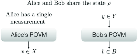
Figure 2: Transforming a PM scenario to a Bell scenario.

The Bell correlation corresponding to the strategy described above is given by $r(x,b|y)=q_{x}\,{p(b|x,y)}$. Applying the lower bounds (1) and (2) to the Bell correlation $r$, we get two lower bounds on $\mathcal{D}(p)$. It can be shown that one of the bounds always dominates the other, so in the theorem we only give the larger of the two, which completes the proof.

Some remarks on the lower bound (3) are in order. Obviously, since $\mathcal{D}(p)$ is integral, we can round the quantity (3) up if it is not an integer. Also one would naturally want to identify a probability distribution $q$ that maximizes (3). In general, finding the probability distribution maximizing (3) corresponds to minimizing a non-convex quadratic function over the set of probability vectors (called the simplex). It is known that solving such a problem is NP-hard MS . However, any probability vector $q$ does yield a lower bound on $\mathcal{D}(p)$. In this work, we mostly consider the uniform distribution, i.e., $q_{x}=1/N$ for all $x\in X$. As it turns out this simple choice is often sufficient to give tight bounds. Later we give an application where one can analytically prove this is optimal.

Lastly, whenever we have at most four possible preparations, i.e., $N\leq 4$, there exists a tractable algorithm to find the distribution $q$ that maximizes (3). Specifically, in this case the problem amounts to solving a semidefinite program, and this can be done in polynomial time Boyd . For this, we use the fact that quadratic optimization over the simplex can be expressed as a linear conic programming problem over the cone of completely positive matrices BDD+00 . An $n$-by-$n$ matrix is completely positive if it can be written as $\sum_{i=1}^{k}x_{i}x_{i}^{\top}$ (for some $k\geq 1$) where $x_{i}\in\mathbb{R}^{n}_{+}$. However, for $n\leq 4$, an $n$-by-$n$ matrix is completely positive if and only if it is positive semidefinite and has nonnegative entries.

Before discussing applications of our lower bound, we first show it can be tight, even when $q$ is uniform. Consider the toy example where $X=\{0,1\}^{M}$, $Y=\{1,\ldots,M\}$, $B=\{0,1\}$, and the PM correlation given by

$$p(b|x,y)\equiv\delta_{b,{x_{y}}}$$ (4)

where $\delta$ is the Kronecker delta function and $x_{y}$ denotes the $y$’th bit of the bitstring $x\in\{0,1\}^{M}$. Intuitively, this means that given an encoding of the bitstring $x$, measurement can pick out any of the bits perfectly, thus can discriminate the quantum states received perfectly. In this case, our lower bound (3) yields $\mathcal{D}(p)\geq 2^{M}=N$, when $q$ is uniform. This is tight since $\mathcal{D}(p)\leq N$ for any PM correlation.

In the toy example above, we see that there is no way to compress the states, that is, to reduce the dimension below the trivial bound of $N$. It turns out that there is a sufficient condition which follows easily from our main theorem. Since it is always true that

$$\sum_{x}\min_{y}\Big{(}\sum_{b}\sqrt{{p(b|x,y)}}\sqrt{{p(b|x,y)}}\Big{)}^{2}=N,$$ (5)

by setting $q$ to be uniform and applying our lower bound (3), we get the following sufficient condition for the impossibility of quantum compressibility, i.e., ${\mathcal{D}(p)=N}$:

$$\forall x\neq x^{\prime},\exists y,\forall b\text{ it holds that }p(b|x,y)\,p(b|x^{\prime},y)=0.$$ (6)

If (6) holds, $p$ cannot be (quantumly) compressed.

New insights for dimension witness. We now introduce two examples to show that our lower bound provides new insights into the concept of dimension witness.

We have mentioned that when the preparer and the measurer in a PM scenario are independent, nonlinear dimension witnesses have been proposed BQB14 ; LBL+15 . Suppose we have a PM correlation $p$ in the setting of $X=\{0,1,2,3\}$, $Y=\{0,1\}$, and $B=\{0,1\}$. Then the determinant of the following $2\times 2$ matrix

$$W_{2}=\begin{bmatrix}p(0|0,0)-p(0|1,0)&p(0|2,0)-p(0|3,0)\\ p(0|0,1)-p(0|1,1)&p(0|2,1)-p(0|3,1)\end{bmatrix},$$

is a nonlinear dimension witness BQB14 . In BQB14 it was pointed out that if ${\rm det}(W_{2})=2$ (the largest value possible), then $\mathcal{D}(p)\geq 4$. It can easily be shown that this also follows from our sufficient condition for non-compressibility. This is because when the determinant is $2$, all the entries of $W_{2}$ must be $1$ or $-1$. Then one can check that the conditions (6) are met, and we get $\mathcal{D}(p)=4$.

For our second example, we recover the dimension witness in BNV13 . Specifically, we show something slightly more general, that for $K=2$ and any $M$, $N$, we have that

$$\sum_{x,x^{\prime}}\max_{y}\left|p(1|x,y)-p(1|x^{\prime},y)\right|^{2}\leq\Big{(}1-\frac{1}{d}\Big{)}N^{2}$$ (7)

is a quadratic dimension witness for $d<N$. This can be easily shown by applying the Fuchs-van de Graaf inequalities FG99 to our lower bound (3) (with $q$ uniform).

Note that in BNV13 , the dimension witness (7) was derived in the special case $M=N(N-1)/2$. In this case, the measurements $y$ in (7) are fixed and labelled by $y=(x,x^{\prime})$, $x>x^{\prime}$. It turns out that in this case, (7) can be tight BNV13 .

Relation to the Positive Semidefinite rank (PSD-rank). We first consider the case $M=1$, i.e., the measurer has only one choice of measurement. For this, we introduce the $N$-by-$K$ row stochastic matrix $Q$ with entries given by $p(b|x)$. In this case, it is known LWdW14 that $\mathcal{D}(p)$ is equal to the PSD-rank of $Q$, denoted $\mbox{\tt{rank}}_{psd}(Q)$, defined as the least integer $c\geq 1$ such that there exist ${c\times c}$ positive semidefinite matrices matrices $E_{1},\ldots,E_{N},F_{1},\ldots,F_{K}$ satisfying $Q_{x,b}=\mathrm{Tr}(E_{x}F_{b}),\textup{ for all }x,b$. The PSD-rank is an important quantity in computer science and mathematical optimization FMP+12 ; GPT13 ; LSR14 .

We can expand this idea to more measurements in a few ways. First, in LWdW14 it was shown that $\mbox{\tt{rank}}_{psd}(Q)\geq\sum_{b}\max_{x}\,Q_{x,b}$ (this holds for any entry-wise nonnegative matrix Q). Applying this to each $y$ individually, we get

$$\mathcal{D}(p)\geq\max_{y}\sum_{b}\max_{x}\,p(b|x,y),$$ (8)

which was also observed in SH14 . Notice that the lower bound (8) is always upper bounded by $K$. Thus, our lower bound (3) can vastly outperform this bound as can be seen by the PM correlation (4). Second, we can consider the matrix $Q$ to the $KM$-by-$N$ matrix $Q^{\prime}$ with entries given by $Q^{\prime}_{(y,b),x}=p(b|x,y)$. By definition, it follows that $\mathcal{D}(p)\geq\mbox{\tt{rank}}_{psd}(Q^{\prime})$. Then using the technique to lower bound PSD-rank introduced in LWdW14 , we can recover (3), giving an alternative proof of our main result.

Quantum random access codes. We now consider the PM correlations arising from an information task known as random access coding. The goal here is to encode $M$ bits into a quantum state of hopefully small dimension such that the measurer can choose any of the $M$ bits to learn with high probability. Moreover, consider a PM scenario with $X=\{0,1\}^{M}$, $Y=\{1,\ldots,M\}$, and $B=\{0,1\}$ where the PM correlation is given by

$$p(b|x,y)\equiv\left\{\begin{array}[]{cl}\beta&\text{ if }b=x_{y},\\ 1-\beta&\text{ if }b\neq x_{y}.\end{array}\right.$$ (9)

Here $\beta\geq 1/2$ is the success probability of learning the $y$’th bit correctly. There are well-known examples where a single qubit can encode $2$ bits with $\beta\approx 0.8536$ (see BBBW83 ; ANTV99 ) or $3$ bits with $\beta\approx 0.7887$ (see Chuang ; ANTV02 ). We see that on both these examples, the bound (3) is tight (when $q$ is uniform). In fact, it can be shown that $q$ being uniform is the optimal choice when applying our lower bound (3) for this case of random access codes footnote1 .

We now ask the question of how the dimension is affected when $\beta$ changes. We compare our bound to Nayak’s bound Nay99 , which is essentially optimal and states that a random access code requires at least $(1-H(\beta))M$ qubits, where $H$ is the binary entropy function $H(\beta)\equiv-\beta\log_{2}(\beta)-(1-\beta)\log_{2}(1-\beta)$. In other words, Nayak’s bound can be expressed as ${\mathcal{D}(p)\geq\lceil 2^{(1-H(\beta))M}\rceil}$.

For small values of $M$, our bound behaves very well by being quite close to Nayak’s bound. For example, for $M=2$, Nayak’s bound beats our bound for $\beta\in(0.8900,0.9083)\cup(0.9674,0.9714)$. For all the other values of $\beta$ we get the same bound. Thus, our bound performs very well and is close to optimal in this setting.

However, Nayak’s bound is concerned with the worst case probability of correctly decoding a bit. Therefore, one can easily construct other PM correlations where our lower bound is greater. For example, if we alter only a few of the states in a random access code such that for some $x$, some of the bits are decoded with a very small success probability, Nayak’s bound will approach $1$ (as the binary entropy will approach $1$). On the other hand, our bound can still be large as it deals with all of the outcome probabilities independently.

Witnessing the non-convexity of restricted-dimensional PM correlations. We now study the sets of restricted-dimensional PM correlations, that is, the sets ${D_{d}\equiv\{p:\mathcal{D}(p)\leq d\}}$, for some fixed integer $d\geq 1$. It was first pointed out in GBHA10 that there exist choices for $d$ for which ${D}_{d}$ is not convex. We now show that this can be proved easily using the lower bound (3).

For this, consider the PM scenario with $X=\{0,1\}^{2}$, $Y=\{1,2\}$, and $B=\{0,1,2\}$. For $i=1,2$ define

$$p_{i}(b|(x_{1},x_{2}),y)\equiv\left\{\begin{array}[]{cl}\delta_{b,x_{i}}&\text{ if }y=i\\ \delta_{b,2}&\text{ if }y\neq i.\end{array}\right.$$ (10)

Intuitively, this is similar to our toy example (4) where one wants to perfectly decode one of two bits, except that the measurer can output “I am not certain” (as indicated by the outcome “$2$”). Then $p_{i}$ is the PM correlation where the preparer chooses two bits $(x_{0},x_{1})$, sends $x_{i}$, and the measurer learns and outputs $x_{i}$ if and only if $y=i$ (and outputs “$2$” otherwise). For this reason, it is clear that each $p_{i}$ is in $D_{2}$.

The convex combination is more than just sending a random choice of $x_{1}$ or $x_{2}$ as the measurer’s POVMs need to be taken into account. It turns out that any qubit encoding is not possible as our lower bound (3) applied to $\frac{1}{2}p_{1}+\frac{1}{2}p_{2}$ (with $q$ uniform) is equal to $16/7>2$. Therefore, $\frac{1}{2}p_{1}+\frac{1}{2}p_{2}\not\in D_{2}$, witnessing that $D_{2}$ is not convex.

Conclusions. In this work we derived a lower bound for the dimension of any quantum system that can produce a given PM correlation, which is applicable to any choice of parameters, and has nontrivial applications. Specifically, we showed that our lower bound provides new insights for the notion of dimension witness. We also used the bound to prove that the set of restricted-dimension PM correlations is not always convex. Due to the generality of the PM scenario we believe that our lower bound will lead to more nontrivial applications, and will provide new insights into the study of device-independent quantum processing tasks.

- (1) N. Brunner, S. Pironio, A. Acín, N. Gisin, A. A. Méthot, and V. Scarani, Phys. Rev. Lett. 100, 210503 (2008).
- (2) S. Wehner, M. Christandl, A. C. Doherty, Phys. Rev. A 78, 062112 (2008).
- (3) J. Sikora, A. Varvitsiotis, Z. Wei, e-print arXiv:1507.00213v2; to appear in Phys. Rev. Lett.
- (4) N. Brunner, D. Cavalcanti, S. Pironio, V. Scarani, and S. Wehner, Rev. Mod. Phys. 86, 419 (2014).
- (5) R. Gallego, N. Brunner, C. Hadley, and A. Acín, Phys. Rev. Lett. 105, 230501 (2010).
- (6) J. Bowles, M. T. Quintino, N. Brunner, Phys. Rev. Lett. 112, 140407 (2014).
- (7) M. Hendrych, R. Gallego, M. Mičuda, N. Brunner, A. Acín, and J. P. Torres, Nat. Phys. 8, 588 (2012).
- (8) J. Ahrens, P. Badziag, A. Cabello, and M. Bourennane, Nat. Phys. 8, 592 (2012).
- (9) N. Brunner, M. Navascués, T. Vértesi, Phys. Rev. Lett. 110, 150501 (2013).
- (10) Y. Cai, J.-D. Bancal, J. Romero, V. Scarani, e-print arXiv:1606.01602.
- (11) T. Lunghi, J. B. Brask, C. W. Lim, Q. Lavigne, J. Bowles, A. Martin, H. Zbinden, and N. Brunner, Phys. Rev. Lett. 114, 150501 (2015).
- (12) K. T. Goh, J. D. Bancal, V. Scarani, New J Phys. 18, 045022 (2016).
- (13) A. Chailloux, I. Kerenidis, S. Kundu, and J. Sikora, New J Phys. 18, 045003 (2016).
- (14) R. Chaves, J. Brask, N. Brunner, Phys. Rev. Lett. 115, 110501 (2015).
- (15) T.S. Motzkin, E.G. Straus, Canad. J. Math. 17, 533-540 (1965).
- (16) I. Bomze, M. Dür, E. de Klerk, C. Roos, A. J. Quist, and T. Terlaky, J. Global. Optim. 18, 301-320 (2000).
- (17) S. Boyd, L. Vandenberghe, Convex Optimization, Cambridge University Press (2004).
- (18) P. H. Diananda, Proc. Cambridge Philos. Soc. 58, 17-25 (1962).
- (19) T. Lee, Z. Wei, R. de Wolf, e-print arXiv:1407.4308, to appear in Math. Program.
- (20) C. J. Stark, A. W. Harrow, IEEE Trans. Inf. Theory 62, 2867-2880 (2016).
- (21) C. A. Fuchs, J. van de Graaf, IEEE Trans. Inf. Theory 45, 1216-1227 (1999).
- (22) S. Fiorini, S. Massar, S. Pokutta, H.R. Tiwary, and R. de Wolf, In Proceedings of the 44th ACM STOC, pages 95-106, 2012.
- (23) J. Gouveia, P. Parrilo, R. Thomas, Math. Oper. Res. 38, 248 (2013).
- (24) J. Lee, D. Steurer, P. Raghavendra, In Proceedings of the 47th ACM STOC, pages 567-576, 2015.
- (25) C. Bennett, G. Brassard, S. Breidbard, and S. Wiesner, Advances in Cryptology CRYPTO 1982, pages 267-275, 1983.
- (26) A. Ambainis, A. Nayak, A. Ta-Shma, and U. Vazirani, In Proceedings of the 31st ACM STOC, pages 376-383, 1999.
- (27) I. Chuang, unpublished result, 1997.
- (28) A. Ambainis, A. Nayak, A. Ta-Shma, and U. Vazirani, Journal of the ACM, 49(4):496-511 (2002).
- (29) The quadratic optimization problem of finding the distribution maximizing (3) turns out to be convex in this case and furthermore, using the Karush-Kuhn-Tucker conditions (e.g. see Boyd ), it can be verified that the optimal is uniform.
- (30) A. Nayak, In Proceedings of the 40th IEEE Symposium on Foundations of Computer Science, pages 369-376, 1999.