Do hydrodynamically assisted binary collisions lead to orientational ordering of microswimmers?

Abstract

We have investigated the onset of collective motion in systems of model microswimmers, by performing a comprehensive analysis of the binary collision dynamics using three dimensional direct numerical simulations (DNS) with hydrodynamic interactions. From this data, we have constructed a simplified binary collision model (BCM) which accurately reproduces the collective behavior obtained from the DNS for most cases. Thus, we show that global alignment can mostly arise solely from binary collisions. Although the agreement between both models (DNS and BCM) is not perfect, the parameter range in which notable differences appear is also that for which strong density fluctuations are present in the system (where pseudo-sound mound can be observedOyama et al. (2016)).

I Introduction

Active matter encompasses a vast range of systems, from microorganisms at the microscopic scale, to humans and other mammals at the macroscopic scaleVicsek and Zafeiris (2012); Marchetti et al. (2013). These active systems can show various nontrivial collective behaviors Lushi et al. (2014); Ezhilan et al. (2013); Oyama et al. (2016); Chaté et al. (2008); Bazazi et al. (2008); Buhl et al. (2006); Zöttl and Stark (2016). Especially striking is the global ordering in the absence of any external field or leading agentsBallerini et al. (2008); Volfson et al. (2008); Lukeman et al. (2010); Schaller et al. (2010); Evans et al. (2011). In order to validate the various scenarios that have been proposed to explain such phenomena, it is important to develop model systems which can be well-controlled experimentally and efficiently simulated. For this purpose, micro-swimmers, such as microbes and self-propelled Janus particles, have been extensively used. It is known that hydrodynamic interactions can play a dominant role in the dynamics of microswimmers dispersionsRafaï et al. (2010). For example, in ref. Lushi et al. (2014), the authors study the dynamics of confined bacterial suspensions, and found that they could reproduce the experimentally observed results with simulations, but only if hydrodynamic interactions were taken into account. While the experimental realizations can be rather complicated, simple computational models exist which allow for direct numerical calculations, such that the hydrodynamic effects can be accurately represented. Indeed, several simulation works on model microswimmer dispersions have recently been performed in order to study the role of hydrodynamicsOyama et al. (2016); Evans et al. (2011); Kyoya et al. (2015); Alarcón Oseguera (2015); Alarcón and Pagonabarraga (2013); Zöttl and Stark (2014); Li and Ardekani (2014); Navarro and Fielding (2015); Matas-Navarro et al. (2014); Ishikawa and Pedley (2014); Ishikawa et al. (2010); Giacché and Ishikawa (2010); Ishikawa and Pedley (2008, 2007a, 2007b); Ishikawa et al. (2006); Ishikawa and Hota (2006); Molina et al. (2013); Sano et al. (2016). Of particular interest for our current work is the study by Evans et al.Evans et al. (2011), who investigated the conditions under which polar order appears. They used a common microswimmer model called the squirmer model, which allows one to easily consider different types of swimmers, namely, pushers, pullers and neutral swimmers. They found that the ordering does not depend strongly on the volume fraction of swimmers, but rather on the type and strength of the swimming. The fact that we observe ordering in very dilute dispersions suggests that the mechanisms leading to the collective alignment do not depend on the volume fraction, and could be explained by considering only binary collisions. Thus, in this work we investigate the onset of polar ordering by performing a detailed analysis of the collision data obtained from three dimensional (3D) simulations of swimmer suspensions with hydrodynamic interactions. First, we have extended the study of Evans’ et al., by performing direct numerical simulations (DNS) of bulk suspensions over a larger set of parameters. We have confirmed that the volume fraction dependence is weak if the volume fraction is small enough (if it is high, the polar order collapses). Second, by simulating binary particle collision events with varying collision geometries, we have gathered comprehensive information on the changes in swimming direction that a particle feels when it undergoes a collision. If we look at changes in the relative angles of two particles after the collisions, the results show different tendencies depending on the type of swimmer. Pullers tend to exhibit disalignment when the incoming relative angle is small, while pushers exhibit disalignment at intermediate values. Furthermore, using this binary collision data, we have constructed a simple binary collision model (BCM) and used it to study the collective alignment of many particle systems as a function of swimming type. The BCM successfully reproduced the emergence of the polar order except for dispersions of intermediate pullers for which a strong clustering behavior is reportedOyama et al. (2016); Alarcón and Pagonabarraga (2013).

II Simulation Methods

II.1 The Squirmer Model

In this work, the squirmer model was used to describe the swimmersLighthill (1952); Blake (1971). Squirmers are particles with modified stick boundary conditions at their surface which are responsible for the self-propulsion. The general form is given as an infinite expansion of both radial and tangential velocity components, but for simplicity the radial terms are usually neglected and the infinite sum is truncated to second orderIshikawa and Pedley (2007a). For spherical particles, the surface velocity is given by

$$\boldsymbol{u}^{s}(\theta)=B_{1}\left(\sin{\theta}+\frac{\alpha}{2}\sin{2\theta}\right)\hat{\boldsymbol{\theta}},$$ (1)

where $\hat{\boldsymbol{\theta}}$ and $\hat{\boldsymbol{r}}$ (we use a caret to denote unit vectors) are the tangential and radial unit vectors for a given point at the surface of the particle and $\theta=\cos^{-1}{(\hat{\boldsymbol{r}}\cdot\hat{\boldsymbol{e}})}$ is the polar angle (since the system is axisymmetric around the swimming direction $\hat{\boldsymbol{e}}$, the azimuthal angle does not appear). The steady-state swimming velocity is determined only by the coefficient of the first mode $B_{1}$ (the source dipole), and the ratio of the first two modes $\alpha=B_{2}/B_{1}$ determines the type and strength of the swimming. When $\alpha$ is negative, the squirmers are pushers, and generate extensile flow fields, and when it is positive, they are pullers and generate contractile flow fields. For the special case when $\alpha=0$, we refer to the swimmers as a neutral swimmer which is accompanied by a potential flow. The difference in the type of swimmer can be related to the position of the propulsion mechanism along the body. A swimmer whose propulsion is generated at the back is a pusher (e.g. E. Coli), one whose propulsion comes from the front is a puller (e.g., Chlamydomonas Reinhardtii). The former will generate an extensile stress, the latter a contractile stress. In contrast, for neutral swimmers such as Volvox the dipole term is dominant ($B_{2}\ll B_{1}$), resulting in a symmetric flow field with no vorticity. Approximate values for $\alpha$ of real swimmers have been reported as $\alpha\approx-1$ for E. Coli, $\alpha\approx 1$ for Chlamydomonas and $\alpha\approx 0$ for VolvoxEvans et al. (2011). In what follows, we refer to $\alpha$ as the swimming parameter.

II.2 Smoothed Profile Method

In order to solve for the dynamics of squirmers swimming in a viscous host fluid, the coupled equations of motion for the fluid and the solid particles need to be considered. Particles follow the Newton-Euler equations of motion:

$$\dot{\boldsymbol{R}}_{i} =\boldsymbol{V}_{i} \dot{\boldsymbol{Q}}_{i} =\text{skew}(\boldsymbol{\Omega}_{i})\cdot\boldsymbol{Q}_{i}$$ (2)

$$M_{\text{p}}\dot{\boldsymbol{V}}_{i} =\boldsymbol{F}_{i}^{\text{H}}+\boldsymbol{F}_{i}^{\text{C}} \boldsymbol{I}_{\text{p}}\cdot\dot{\boldsymbol{\Omega}}_{i} =\boldsymbol{N}_{i}^{\text{H}}$$

where $i$ is the particle index, $\boldsymbol{R}_{i}$ the position, $\boldsymbol{Q}_{i}$ the orientational matrix, and $\text{skew}(\boldsymbol{\Omega}_{i})$ the skew symmetric matrix of the angular velocity $\boldsymbol{\Omega}_{i}$. The hydrodynamic force $\boldsymbol{F}_{i}^{\text{H}}$ and torque $\boldsymbol{N}_{i}^{\text{H}}$ are computed assuming momentum conservation to guarantee proper coupling between the fluid and the particles. To prevent particles from overlapping, we have also included an excluded volume effect by introducing a repulsive interaction between particles, $\boldsymbol{F}_{i}^{\text{C}}$, as a truncated Lennard-Jones potential with (36-18) powers. Therefore, particles interact with each other both via long-range hydrodynamic interactions and the short-range repulsive force. We note that the exact form of the short-range repulsive force is not crucial for the dynamics of non-Brownian particlesDratler and Schowalter (1996). The time evolution of the fluid flow field is governed by the Navier-Stokes equation with the incompressible condition:

$$\boldsymbol{\nabla}\cdot\boldsymbol{u}_{\rm f} =0$$ (3)

$$\rho_{\text{f}}\left(\partial_{t}+\boldsymbol{u}_{\text{f}}\cdot\nabla\right)\boldsymbol{u}_{\text{f}} =\nabla\cdot\boldsymbol{\sigma}_{\rm f}$$ (4)

$$\boldsymbol{\sigma}_{\rm f} =-p\boldsymbol{I}+\eta_{\rm f}\left\{\nabla\boldsymbol{u}_{\text{f}}+\left(\nabla\boldsymbol{u}_{\text{f}}\right)^{t}\right\}$$ (5)

where $\rho_{\text{f}}$ is the fluid mass density, $\eta_{\rm f}$ the shear viscosity, and $\boldsymbol{\sigma}_{\rm f}$ is the Newtonian stress tensor. To couple these equations efficiently, we have used the Smoothed Profile Method (SPM), which enables us to calculate the solid/fluid two-phase dynamics on fixed grids with hydrodynamic interactionsNakayama and Yamamoto (2005); Kim et al. (2006); Nakayama et al. (2008); Molina et al. (2013). In the SPM, the sharp interface between the solid and fluid domains is replaced by a diffuse one with finite width $\xi$, and the solid phase is represented by a smooth and continuous profile function $\phi_{\rm p}$. This profile function takes a value of 1 in the solid domain, and 0 in the fluid domain. By introducing the smoothed profile function, we can define a total velocity field, $\boldsymbol{u}$, which includes both fluid and particle velocities, and is defined over the entire computational domain, as:

$$\boldsymbol{u}=\left(1-\phi\right)\boldsymbol{u}_{\rm f}+\phi\boldsymbol{u}_{\rm p},$$

$$\phi\boldsymbol{u}_{\rm p}=\sum_{i}\phi_{i}\left[\boldsymbol{V}_{i}+\boldsymbol{\Omega}_{i}\times\boldsymbol{R}_{i}\right],$$ (6)

where, $\left(1-\phi\right)\boldsymbol{u}_{\rm f}$ is the contribution from the fluid, $\phi\boldsymbol{u}_{\rm p}$ from the particle motion. The time evolution of the total flow field $\boldsymbol{u}$ obeys:

$$\boldsymbol{\nabla}\cdot\boldsymbol{u} =0,$$

$$\rho_{\text{f}}\left(\partial_{t}+\boldsymbol{u}\cdot\nabla\right)\boldsymbol{u} =\nabla\cdot\boldsymbol{\sigma}_{\rm f}+\rho_{\rm f}\left(\phi\boldsymbol{f}_{\rm p}+\boldsymbol{f}_{\rm sq}\right)$$ (7)

where $\phi\boldsymbol{f}_{\text{p}}$ is the body force necessary to maintain the rigidity of particles, and $\boldsymbol{f}_{\text{sq}}$ is the force due to the active squirming motion. This method drastically reduces the computational cost.

III Results

III.1 Bulk Polar Order

To start, we used the SPM to carry out DNS studies of bulk swimmer dispersion in 3D at varying volume fraction $\varphi$ and swimming type $\alpha$. We use a cubic system of linear dimension of $64\Delta$, with $\Delta$ the grid spacing. The viscosity and the mass density of the host fluid, $\mu$, $\rho_{f}$ are set to one, such that the unit of time is $t_{0}=\rho_{f}\Delta^{2}/\mu$. The particle diameter $\sigma$ and the interface thickness $\xi$ are $4\Delta$ and $2\Delta$ respectively. We used a random initial configuration for the particle positions and orientations, and varied the number of particles $N_{\rm p}$ from $500$ to $4000$, which correspond to a range of volume fraction $0.06\lesssim\varphi\lesssim 0.5$. To quantify the degree of collective alignment, we calculate the polar order parameter $P$Evans et al. (2011); Alarcón and Pagonabarraga (2013)

$$P=\left\langle\frac{1}{N_{\rm p}}\left|\sum_{i}^{N_{\rm p}}\hat{\boldsymbol{e}}_{i}\right|\right\rangle,$$ (8)

where $\hat{\boldsymbol{e}}_{i}$ is the swimming direction of particle $i$, $N_{\rm p}$ the number of particles and angular brackets denote an average over time (after steady state has been reached). Typical simulation snapshots for disordered ($P\simeq 0$) and ordered ($P\simeq 1$) systems are given in Fig. 1(a). We note that even for a completely random distribution of orientations, the polar order defined by Eq. (8) will not be exactly $0$, and will depend slightly on the number of particles, as $P_{0}=1/\sqrt{N_{\rm p}}$, where $P_{0}$ represents the polar order value below which we can consider the system is in an isotropic phase.

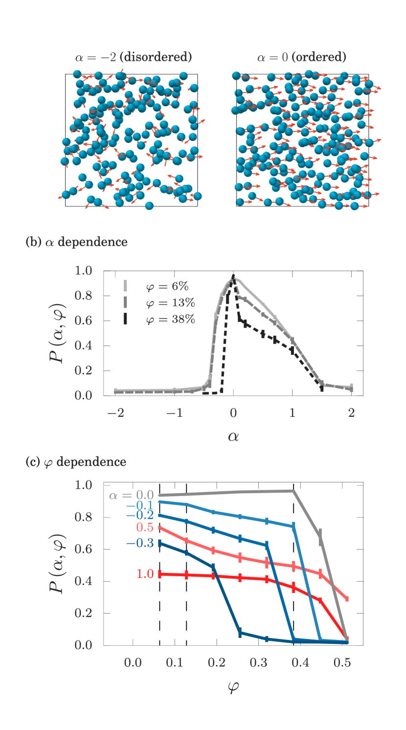
Figure 1: (a) Simulation snapshots for disordered ($\alpha=-2$) and ordered ($\alpha=0$) states. The arrows give the direction of motion, and only a subset of the particles have been drawn. (b) The $\alpha$ dependency of the polar order $P\left(\alpha,\varphi\right)$ for $\varphi=6\%$ (solid line), $13\%$ (light dashed line) and $38\%$ (dark dashed line). (c) The $\varphi$ dependency of $P\left(\alpha,\varphi\right)$ for several values of $\alpha$. Dashed vertical lines indicate the volume fractions of $6,13$ and $38\%$ used in (a) and (b).

The polar order parameter $P$ is a function of only the volume fraction of particles $\varphi$ and the swimming parameter $\alpha$Evans et al. (2011). First, we investigated $\alpha$ dependency. The results are illustrated in Fig. 1(b), for volume fractions $\varphi=6\%$ ($N_{\rm p}=500$),$13\%$ ($N_{\rm p}=1000$) and $38\%$ ($N_{\rm p}=3000$). All the results show a similar tendency and are in agreement with preceding worksEvans et al. (2011); Alarcón and Pagonabarraga (2013): $P$ has a maximum at $\alpha=0$, independent of $\varphi$, and decreases with increasing value of $\left\lvert{\alpha}\right\lvert$. In addition, the $P$ for pushers decays faster than that of pullers as the magnitude of $\alpha$ is increased. For non-pusher $\alpha\geq 0$, the volume fraction dependence of $P$ is not very large and at least the qualitative ordering tendency is the same; but for weak pushers (for example $\alpha\approx-0.3$), we observe a significant drop in the value of $P$, or an order/disorder phase transition when the volume fraction increases. The volume fraction dependence can be seen clearly in Fig. (1c), where we have plotted the values of $P$ over the entire volume fraction range for six different swimmers ($\alpha=-0.3,-0.2,-0.1,0,0.5,1$). Evans et al. have previously reported such a volume fraction dependence for $\alpha=1$ Evans et al. (2011). To understand the dependence of $P$ on the swimming type $\alpha$, in particular the different behaviors seen for pushers and pullers, it is useful to compare them against the results obtained for neutral swimmers $\alpha=0$, which show the highest degree of alignment. As seen in Figure1 (c), the order parameter for $\alpha=0$ shows two distinct regimes: for $\varphi\lesssim 0.4$ there is little variation; for $\varphi\gtrsim 0.4$ there is a drastic drop in the order parameter to $P=0~{}(P_{0})$. The same behavior is observed for pushers, although both of the degree of ordering and the critical volume fraction $\varphi_{c}$ (where the order parameter falls to zero) are both reduced (higher $\left\lvert{\alpha}\right\lvert$ resulting in lower $P$ and $\varphi_{c}$). In contrast, pullers show a gradual decrease only in the degree of order depending on $\left|\alpha\right|$. Interestingly, intermediate pullers ($\alpha=0.5$) maintain a non-zero order parameter over the entire volume fraction range we have considered (all other systems giving $P\approx P_{0}$ at the highest $\varphi$). We believe this anomalous behavior for the intermediate pullers can be related to the strong clustering behavior that gives rise to density inhomogeneitiesOyama et al. (2016); Alarcón and Pagonabarraga (2013). Note that because the number of particles are sufficiently large (even for the system with the smallest volume fraction which corresponds to $N_{\rm p}=500$, the value of $P_{0}$ is less than 0.05), the decays in $P$ are not related to the fact that we use different values of $N_{\rm p}$. We note that continuum theories predict an unstable long wave-length ordering, with no global order in the limit of infinitely large systemsAditi Simha and Ramaswamy (2002). However, we consider that the finite size effects, if they exist, will not lead to qualitatively different results. This is supported by the fact that the pair distribution function decays very fast for most squirmer dispersions (see Supplemental Material). Only in the case of pullers do we measure a long-range correlation which might suffer from finite size effects. In fact, these effects were studied in detail by AlarcónAlarcón Oseguera (2015), who nevertheless showed that the polar order converges to a non-zero value as the system size is increased. The discrepancies with the continuum predictions are likely due to the absence of the finite particle volume term in such theories, which only take into account the long-range hydrodynamic interactions. While these long-ranged interactions tend to destabilize the global ordering, in squirmer dispersions they are screened by neighboring particles, allowing the system to maintain its order, even for very large systems.

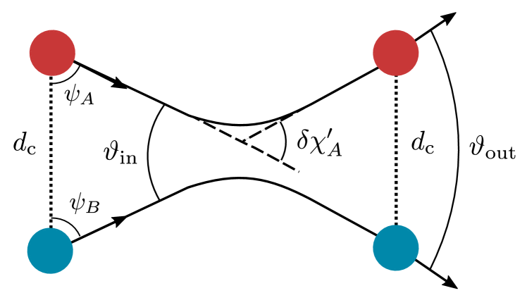
Figure 2: Schematic representation of the collision geometry.

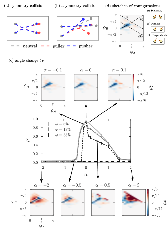
Figure 3: (a-b) Typical trajectories of collisions of neutral swimmer ($\alpha=0$; colored as gray), pullers ($\alpha=0.5$; red) and pushers ($\alpha=-0.5$; blue) for (a) a symmetric collision and (b) an asymmetric one. (c) Change in the relative angle between the particles during collisions, $\delta\vartheta=\vartheta_{\rm out}-\vartheta_{\rm in}$, as a function of the initial orientations, $\psi_{\rm A}$ and $\psi_{\rm B}$. Results of bulk polar order measurement are also shown ($\varphi=6,13$ and $38\%$). In intensity maps, red colors mean positive values or the disalignment effect and blue colors negative or the aligning effect. (d) Sketches for the characteristic configurations in the intensity maps in (c).

III.2 Binary Collision Analysis

Taking into account the fact that at low volume fractions, two body interactions are dominant, we can expect that the observed polar order in bulk is due to binary collisions. This is supported by the fast decay in the spatial correlations of the particle velocities. In the Supplemental Material, we show results for the velocity correlations of systems at $\varphi=0.06$ for both squirmers and inert sedimenting colloids. For the squirmers, regardless of the swimming parameter $\alpha$, the correlation is nonzero only in the close vicinity of the particle, while the correlation length for the colloidal systems extends to several particles diameters. Such short-ranged correlations for swimmers at low volume fractions suggest that only binary collisions can lead to the polar order observed in bulk. To verify the hypothesis proposed above, we first conducted an intensive analysis on the binary collision of squirmers with varying values of $\alpha$. For this, we conducted simulations with only two squirmers in a quasi two-dimensional setup, where particles are confined to a 2D plane, while the computational domain is fully three dimensional. Then, we tried to construct a simplified binary collision model (BCM) using the data obtained by this analysis. We note that a similar binary collision analysis for pullers has been done by Ishikawa et al.Ishikawa et al. (2006). We have extended their work to pushers and neutral swimmers and made direct comparison between the BCM and the bulk DNS results.

We have carried out 3D DNS for a pair of particles with various collision geometries and $\alpha$ values. Given the symmetry of the problem, the two particles will move in a 2D plane (defined by the two orientation vectors). We considered collisions of two particles labeled $A$ and $B$. The precise parametrization we have used to describe the collision is given in Fig. 2, where three sets of angles have been defined, $\psi_{j}$, $\delta\chi_{j}$ ($j\in\left\{A,B\right\}$ is the particle label) and $\vartheta_{\rm in/out}$. The initial configuration of the system is specified by $\psi_{j}$, the angles between the direction of motion and the center-to-center distance vector at the initial state. These angles determine whether particles start swimming towards or away from each other. The information for the change in the swimming direction of each particle is given by $\delta\chi_{j}$. Then, the relative orientation of particles when the collision event starts/ends is represented by $\vartheta_{\rm in/out}$. Due to the long-range nature of the hydrodynamic interactions, particles can alter their directions even without touching, in contrast to collisions in a gas of hard-sphere particles. Therefore, there is no unique way to define a “collision” between particles. In this work, we define a characteristic distance $d_{c}$ that is the threshold distance under which particles are considered to be colliding: a collision event has started when the distance between the two particles becomes less than $d_{c}$, and it lasts until the distance exceeds this value (see Figure 2). Thus, $d_{c}$ should be large enough that hydrodynamic interactions can be neglected when the distance between the particles exceeds $d_{c}$.

The parameters for the binary collision is determined as follows. The initial particle distance was set to $d_{0}=16\Delta=4\sigma$, and the collision threshold to $d_{c}=15\Delta$. The value of $d_{c}$ is determined to be big enough so that we can safely ignore the hydrodynamic interactions if the particle-particle distance is greater than $d_{c}$ (above this value, particles hardly change their orientations). The value of $d_{0}$ is determined so that swimmers have obtained their steady state velocity when the inter-particle distance becomes $d_{c}$. The initial geometry was varied by changing $\psi_{j}$ in intervals of $\pi/12$, for $0\leq\psi_{A}\leq\pi$ and $-\pi\leq\psi_{B}\leq\pi$. To take into account the symmetry of the system, we label one of the particles ($A$) as a reference particle, and take $\psi_{A}\geq 0$, while $\psi_{B}$ is defined as

$$\psi_{B} =\operatorname{\mathrm{sign}}{\left(\mathcal{P}_{AB}\cdot\hat{\boldsymbol{e}}_{A}\right)}\operatorname{\mathrm{sign}}{\left(\mathcal{P}_{AB}\cdot\hat{\boldsymbol{e}}_{B}\right)}\left\lvert{\arccos{\left(\hat{\boldsymbol{r}}_{AB}\cdot\hat{\boldsymbol{e}}_{B}\right)}}\right\lvert$$ (9)

where $\boldsymbol{r}_{AB}=\boldsymbol{r}_{B}-\boldsymbol{r}_{A}$, $\mathcal{P}_{AB}$ is the projection operator (with $\mathcal{I}$ the identity operator)

$$\mathcal{P}_{AB} =\mathcal{I}-\hat{\boldsymbol{r}}_{AB}\hat{\boldsymbol{r}}_{AB}$$ (10)

and $\operatorname{\mathrm{sign}}(x)=1$ for $x\geq 0$ and $\operatorname{\mathrm{sign}}(x)=-1$ for $x<0$. As mentioned above, we use a caret to denote unit vectors. Thus, $\psi_{B}$ is defined as positive if both particles are swimming towards the same side with respect to the center-to-center line between particles. We note that only combinations of $\psi_{j}$ which meet $\hat{\boldsymbol{e}}_{AB}\cdot\hat{\boldsymbol{r}}_{AB}<0$ can lead to “collisions”, where $\boldsymbol{e}_{AB}=\hat{\boldsymbol{e}}_{B}-\hat{\boldsymbol{e}}_{A}$. Three-dimensional simulations for the binary collision were performed using the same system parameters as for the bulk simulations presented above.

The results of the binary collision analysis are summarized in Fig. 3. Fig. 3(a) and (b) show typical trajectories and Fig. 3(c) shows changes in the relative angle between the swimming direction of the two particles after the collisions, $\delta\vartheta=\vartheta_{\rm out}-\vartheta_{\rm in}$. In the following, we define a symmetric collision as a collision in which $\psi_{A}=\psi_{B}$ (Fig. 3(a)). Intensity maps show the values of $\delta\vartheta$ as a function of the initial angles, $\psi_{j}$. In Fig. 3(d), the schematic representations of three characteristic initial configurations are shown: (i) symmetric, (ii) parallel, (iii) perpendicular. Although the parallel configuration does not lead to a collision, it is useful to identify the corresponding region in the intensity plots shown in Fig. 3(c). The values of the polar order in bulk are again shown to make the connection between the bulk and binary collision dynamics clear. As shown in Fig. 3 (a) and (b), different values of $\alpha$ lead to different particle trajectories, resulting in different patterns for $\delta\vartheta$ (Fig. 3 (c)). The results of $\delta\vartheta$ in systems of pushers and pullers can be easily understood by considering their deviation from the results for neutral swimmers ($\alpha=0$). The neutral swimmers show strong aligning behaviors only when the collision is symmetric, and just small absolute values of $\delta\vartheta$ otherwise. If we look at the results for pullers ($\alpha>0$), we can perceive that, in the case of $\alpha=0.1$, disalignment effects are detected at small relative incoming angles. Such disalignment effects becomes stronger with the increase in the absolute value of $\alpha$, as shown in the subplots for $\alpha=0.5,2$. On the other hand, in the cases of pushers ($\alpha<0$), disalignment effects are seen at relatively large incoming angles. For pushers, as well as for pullers, the increase in the absolute value of $\alpha$ leads to stronger disalignment effect. In this way, measuring only $\delta\vartheta$, we can observe different tendencies between pushers and pullers. These tendencies seem to be a consequence of the complicated hydrodynamic interactions, and it is impossible to understand intuitively from the view point of the flow field which a single swimmer generates.

To implement a simple binary collision model using the collision data obtained from the DNS, it is necessary to measure the changes in the single particle orientations, $\delta\chi_{j}$. For this, from the comprehensive DNS data for binary collisions, we have determined $\delta\chi_{j}$ for all the collisions, as

$$\delta\chi_{j}=\arcsin\left(\hat{\boldsymbol{z}}_{\chi}\cdot\left(\hat{\boldsymbol{e}}_{j}^{\rm in}\times\hat{\boldsymbol{e}}_{j}^{\rm out}\right)\right),$$ (11)

where the superscript “in/out” refers to the value at the moment when a collision starts/ends, $\hat{\boldsymbol{z}}_{\chi}=\frac{\hat{\boldsymbol{e}}_{j}^{\rm in}\times\hat{\boldsymbol{e}}_{j^{\prime}}^{\rm in}}{|\hat{\boldsymbol{e}}_{j}^{\rm in}\times\hat{\boldsymbol{e}}_{j^{\prime}}^{\rm in}|}$ and $j^{\prime}$ refers to the particle which is colliding with particle $j$.

Finally, in order to investigate whether the polar order seen in bulk systems can be explained only by binary collisions, we constructed a binary collision model (BCM). Here, we have necessarily introduced two simplifications. First, we assume 2D systems. And second, we consider only binary collisions, and use the statistics of collision angles obtained from the present DNS. Because we are assuming very dilute system such that the information of the position doesn’t matter anymore, the particles have only the information about the orientations. Under these simplifications, we calculated the polar order of the system of BCM using the following simple algorithm. At each step of the simulation, we randomly choose two particles (let’s say particles $i$ and $i^{\prime}$). The selected particles will experience a “collision”, which will change their orientations according to the statistics obtained from the binary collision analysis:

$$\chi_{i}\left(s+1\right) =\chi_{i}\left(s\right)+\delta\chi_{i},$$

$$\chi_{i^{\prime}}\left(s+1\right) =\chi_{i^{\prime}}\left(s\right)+\delta\chi_{i^{\prime}},$$ (12)

$$\chi_{k}\left(s+1\right) =\chi_{k}\left(s\right),$$

where subscript $k$ stands for the particles which are not selected to collide. The values $\delta\chi_{i}$ and $\delta\chi_{i^{\prime}}$ are random numbers generated according to the conditional probability distribution when the relative incoming angle $\vartheta_{\rm in}$ is given: $P\left(\delta\chi_{i},\delta\chi_{i^{\prime}}|\vartheta_{\rm in}\left(i,i^{\prime}\right)\right)$, where $\delta\vartheta\left(i,i^{\prime}\right)$ means the relative incoming angle between particles $i$ and $i^{\prime}$. The conditional probability distribution $P\left(\delta\chi_{i},\delta\chi_{i^{\prime}}|\vartheta_{\rm in}\left(i,i^{\prime}\right)\right)$ is determined by using the results of the binary collision analysis presented above. Because there is the information about only the orientation in the BCM, the orientation update algorithm is based only on the relative incoming angle $\bar{\vartheta}_{\rm in}$, and does not depend on the collision parameter (which cannot be defined in this model system) or other geometrical information. No noise term is included. After a sufficiently large number of collisions, the system reaches a steady state, with a constant polar order. We conducted calculations using this BCM for various values of $\alpha$, while keeping the value of $N_{\rm p}=500$ constant. The results for these simulations are plotted in Fig. (4) as red circles, together with results for the quasi-2D and 3D bulk DNS (dark and light solid lines, respectively). The quasi-2D bulk simulations were included for a fair comparison with the BCM results, since the latter is itself obtained from quasi-2D DNS. The setup for these quasi-2D bulk simulations is as follows. The computational domain is three-dimensional, with linear dimensions $L_{x}=64\sigma,L_{y}=64\sigma$ and $L_{z}=4\sigma$ under full periodic boundary conditions. The remaining parameters are the same as those for the 3D bulk systems. Particles are initially placed within the $x-y$ plane at $z=L_{z}/2$, which we refer to as the center plane. The particles are allowed to rotate only around the $z$-axis, such that their trajectories are confined to this center plane. The number of particles is 500 (the same value used in the BCM calculations), which corresponds to an area fraction of $\varphi^{\rm 2D}\approx 10\%$. We use $\varphi^{\rm 3D}$ for the volume fraction in 3D system and $\varphi^{\rm 2D}$ for the area fraction in quasi-2D system. The BCM results and those from the quasi-2D bulk DNS are in good agreement with each other for non-pullers ($\alpha\leq 0$). Interestingly, the results from the 3D bulk DNS also fit very well those of BCM and the quasi-2D bulk DNS. This implies that the dimensionality does not play a big role in determining the polar order formation in squirmer dispersions. This also indicates that the appearance of polar order can be understood just in terms of binary collision events for non-pullers. For pullers, we see an increasing deviation: the larger $\alpha$ becomes, the larger the deviation becomes. For $\alpha\geq 0.4$, qualitatively different results are obtained: in particular, for the BCM the order has collapsed. Here, let us consider the cause of the discrepancy. The BCM is missing two main aspects which affect the dynamics of swimmers: namely, correlated collisions and many body nature of the hydrodynamic interactions. First, in the BCM, the correlation between collisions and particle positions is neglected and the system dynamics is determined by repeated uncorrelated collisions in which the absolute and relative outgoing angles are drawn from the probability distribution measured from the binary system DNS. In real dense dispersions, on the contrary, a sequence of collisions which one particle experiences can be correlated. Second, the BCM assumes that the interactions can be considered as a superposition of binary collisions and therefore ignores the many body nature of the hydrodynamic interactions, which couples the dynamics of particles in real dispersions. Both these effects are expected to become non-negligible and lead to changes in the probability distribution of outgoing angles when the local density is high. The discrepancy between bulk DNS and the BCM can be understood as indirect evidence for the importance of these multi-particle interactions on the order formation in the case of intermediate pullers. The shaded gray region in Fig. 4 marks the parameter range in which we have observed strong clustering in bulk systemsOyama et al. (2016); indeed, it is precisely in this region where the results do not coincide with the BCM (in Fig.. 5, typical snapshots for the systems with $\alpha=0,\pm 0.5$ in quasi-2D bulk system are shown). Though several efforts have been dedicated to verify the importance of binary collisions to explain the polar order formation for various systems both experimentally and numerically Katz et al. (2011); Hanke et al. (2013); Lam et al. (2015); Suzuki et al. (2015); Hiraoka et al. (2016), the presented work is the first successful attempt to conduct such analysis considering full hydrodynamics.

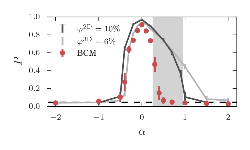
Figure 4: The $\alpha$ dependency of the polar order $P\left(\alpha,\varphi\right)$ for 3D bulk system with $\varphi^{\rm 3D}=6\%$ (light line), quasi-2D bulk system with $\varphi^{\rm 2D}=10\%$ (dark line). Results for the simplified binary collision model are given as circles.

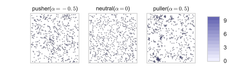
Figure 5: Typical snapshots in quasi-2D bulk systems. The results for the systems with $\alpha=0,\pm 0.5$ are shown. The color represents the number of particles with in the distance of $2\sigma$.

IV Conclusion

Using DNS for squimer dispersions, we have investigated the emergence of polar ordering and its dependency on the particle volume fraction $\varphi$ and swimming strength $\alpha$. In agreement with a previous workEvans et al. (2011), we see that the volume fraction dependence is rather weak, and the ordering depends mostly on $\alpha$ when $\varphi$ is small enough, while at a large value of volume fraction, we observe an order/disorder phase transition. Still, we observed novel volume fraction dependencies for $\left\lvert{\alpha}\right\lvert<1$. In particular, intermediate pullers show no decay of the polar order even at a very high volume fraction, at which all other swimmers show a decay. We believe this anomalous behavior at such a high volume fraction reflects the already-known strong clustering characteristicsOyama et al. (2016); Alarcón and Pagonabarraga (2013). On the other hand, weak pushers show a decay of the polar order even at small volume fractions.

We conducted a detailed analysis of the binary collision dynamics of two swimmers and looked at the changes in the relative orientation of two swimmers after the collisions. The results show different qualitative disaligning tendencies between pusher and puller: pullers show disaligning effects at small relative incoming angles while pushers exhibit at relatively large angles. The absolute value of $\alpha$ changes only the magnitude of disalignment, and the tendency is determined by the sign. Such an analysis also enabled us to construct a simple binary collision model which is able to reproduce the polar ordering seen in the bulk DNS for pushers and neutral swimmers. Thus, it seems binary collisions are enough to explain the appearance of long range polar ordering for these types of swimmers. We note that intermediate pullers exhibit a clear discrepancy between the DNS results and the BCM; however, this occurs in the parameter range where strong clustering behavior is also observed. This can be seen as indirect evidence that in intermediate puller systems, multi-body interactions play an important role. In other words, the origin of the polar order formation can be different, depending on the specific type of swimming. In particular, the mechanism responsible for the clustering of intermediate pullers is still an open question.

V Acknowledgement

We thank N. Yoshinaga, M. Tarama, H. Ito, K. Ishimoto and Simon K. Schnyder for enlightening discussions. This work was supported by the Japan Society for the Promotion of Science (JSPS) KAKENHI Grant No. 17H01083 and also by a Grant-in-Aid for Scientific Research on Innovative Areas “Dynamical ordering of biomolecular systems for creation of integrated functions”(No. 16H00765) from the Ministry of Education, Culture, Sports, Science, and Technology of Japan.

References

- Oyama et al. (2016) N. Oyama, J. J. Molina, and R. Yamamoto, Physical Review E 93, 043114 (2016).
- Vicsek and Zafeiris (2012) T. Vicsek and A. Zafeiris, Physics Reports 517, 71 (2012).
- Marchetti et al. (2013) M. C. Marchetti, J. F. Joanny, S. Ramaswamy, T. B. Liverpool, J. Prost, M. Rao, and R. A. Simha, Reviews of Modern Physics 85, 1143 (2013).
- Lushi et al. (2014) E. Lushi, H. Wioland, and R. E. Goldstein, Proceedings of the National Academy of Sciences 111, 9733 (2014).
- Ezhilan et al. (2013) B. Ezhilan, M. J. Shelley, and D. Saintillan, Physics of Fluids 25, 070607 (2013).
- Chaté et al. (2008) H. Chaté, F. Ginelli, G. Grégoire, F. Peruani, and F. Raynaud, European Physical Journal B 64, 451 (2008).
- Bazazi et al. (2008) S. Bazazi, J. Buhl, J. J. Hale, M. L. Anstey, G. A. Sword, S. J. Simpson, and I. D. Couzin, Current Biology 18, 735 (2008).
- Buhl et al. (2006) J. Buhl, D. J. T. Sumpter, I. D. Couzin, J. J. Hale, E. Despland, E. R. Miller, and S. J. Simpson, Science (New York, N.Y.) 312, 1402 (2006).
- Zöttl and Stark (2016) A. Zöttl and H. Stark, Journal of Physics: Condensed Matter 28, 253001 (2016).
- Ballerini et al. (2008) M. Ballerini, N. Cabibbo, R. Candelier, A. Cavagna, E. Cisbani, I. Giardina, V. Lecomte, A. Orlandi, G. Parisi, A. Procaccini, M. Viale, and V. Zdravkovic, Proceedings of the National Academy of Sciences 105, 1232 (2008).
- Volfson et al. (2008) D. Volfson, S. Cookson, J. Hasty, and L. S. Tsimring, Proceedings of the National Academy of Sciences 105, 15346 (2008).
- Lukeman et al. (2010) R. Lukeman, Y.-x. Li, and L. Edelstein-Keshet, Proceedings of the National Academy of Sciences 107, 12576 (2010).
- Schaller et al. (2010) V. Schaller, C. Weber, C. Semmrich, E. Frey, and A. R. Bausch, Nature 467, 73 (2010).
- Evans et al. (2011) A. A. Evans, T. Ishikawa, T. Yamaguchi, and E. Lauga, Physics of Fluids 23, 111702 (2011).
- Rafaï et al. (2010) S. Rafaï, L. Jibuti, and P. Peyla, Physical Review Letters 104, 098102 (2010).
- Kyoya et al. (2015) K. Kyoya, D. Matsunaga, Y. Imai, T. Omori, and T. Ishikawa, Physical Review E - Statistical, Nonlinear, and Soft Matter Physics 92, 1 (2015).
- Alarcón Oseguera (2015) F. Alarcón Oseguera, PhD. Thesis of Universitat de Barcelona (2015).
- Alarcón and Pagonabarraga (2013) F. Alarcón and I. Pagonabarraga, Journal of Molecular Liquids 185, 56 (2013).
- Zöttl and Stark (2014) A. Zöttl and H. Stark, Physical Review Letters 112, 118101 (2014).
- Li and Ardekani (2014) G.-J. Li and A. M. Ardekani, Physical Review E 90, 013010 (2014).
- Navarro and Fielding (2015) R. M. Navarro and S. M. Fielding, Soft Matter 11, 7525 (2015).
- Matas-Navarro et al. (2014) R. Matas-Navarro, R. Golestanian, T. B. Liverpool, and S. M. Fielding, Physical Review E - Statistical, Nonlinear, and Soft Matter Physics 90, 032304 (2014).
- Ishikawa and Pedley (2014) T. Ishikawa and T. J. Pedley, Physical Review E - Statistical, Nonlinear, and Soft Matter Physics 90, 033008 (2014).
- Ishikawa et al. (2010) T. Ishikawa, J. T. Locsei, and T. J. Pedley, Physical Review E 82, 021408 (2010).
- Giacché and Ishikawa (2010) D. Giacché and T. Ishikawa, Journal of Theoretical Biology 267, 252 (2010).
- Ishikawa and Pedley (2008) T. Ishikawa and T. J. Pedley, Physical Review Letters 100, 088103 (2008).
- Ishikawa and Pedley (2007a) T. Ishikawa and T. J. Pedley, Journal of Fluid Mechanics 588, 437 (2007a).
- Ishikawa and Pedley (2007b) T. Ishikawa and T. J. Pedley, Journal of Fluid Mechanics 588, 399 (2007b).
- Ishikawa et al. (2006) T. Ishikawa, M. P. Simmonds, and T. J. Pedley, Journal of Fluid Mechanics 568, 119 (2006).
- Ishikawa and Hota (2006) T. Ishikawa and M. Hota, The Journal of experimental biology 209, 4452 (2006).
- Molina et al. (2013) J. J. Molina, Y. Nakayama, and R. Yamamoto, Soft Matter 9, 4923 (2013).
- Sano et al. (2016) J.-B. D. Sano, J. Molina, and M, EPL (Europhysics Letters) 114, 24001 (2016).
- Lighthill (1952) M. J. Lighthill, Communications on Pure and Applied Mathematics 5, 109 (1952).
- Blake (1971) J. R. Blake, Journal of Fluid Mechanics 46, 199 (1971).
- Dratler and Schowalter (1996) D. I. Dratler and W. R. Schowalter, Journal of Fluid Mechanics 325, 53 (1996).
- Nakayama and Yamamoto (2005) Y. Nakayama and R. Yamamoto, Physical review. E, Statistical, nonlinear, and soft matter physics 71, 036707 (2005).
- Kim et al. (2006) K. Kim, Y. Nakayama, and R. Yamamoto, Physical Review Letters 96, 1 (2006).
- Nakayama et al. (2008) Y. Nakayama, K. Kim, and R. Yamamoto, European Physical Journal E 26, 361 (2008).
- Aditi Simha and Ramaswamy (2002) R. Aditi Simha and S. Ramaswamy, Physical review letters 89, 058101 (2002).
- Katz et al. (2011) Y. Katz, K. Tunstrom, C. C. Ioannou, C. Huepe, and I. D. Couzin, Proceedings of the National Academy of Sciences 108, 18720 (2011).
- Hanke et al. (2013) T. Hanke, C. A. Weber, and E. Frey, Physical Review E 88, 052309 (2013).
- Lam et al. (2015) K.-D. N. T. Lam, M. Schindler, and O. Dauchot, New Journal of Physics 17, 113056 (2015).
- Suzuki et al. (2015) R. Suzuki, C. A. Weber, E. Frey, and A. R. Bausch, Nature Physics 11, 839 (2015).
- Hiraoka et al. (2016) T. Hiraoka, T. Shimada, and N. Ito, Physical Review E - Statistical, Nonlinear, and Soft Matter Physics 94, 062612 (2016).