Laplacian LRR on Product Grassmann Manifolds for Human Activity Clustering in Multi-Camera Video Surveillance

Abstract

In multi-camera video surveillance, it is challenging to represent videos from different cameras properly and fuse them efficiently for specific applications such as human activity recognition and clustering. In this paper, a novel representation for multi-camera video data, namely the Product Grassmann Manifold (PGM), is proposed to model video sequences as points on the Grassmann manifold and integrate them as a whole in the product manifold form. Additionally, with a new geometry metric on the product manifold, the conventional Low Rank Representation (LRR) model is extended onto PGM and the new LRR model can be used for clustering non-linear data, such as multi-camera video data. To evaluate the proposed method, a number of clustering experiments are conducted on several multi-camera video datasets of human activity, including Dongzhimen Transport Hub Crowd action dataset, ACT 42 Human action dataset and SKIG action dataset. The experiment results show that the proposed method outperforms many state-of-the-art clustering methods.

1 Introduction

For the past decades, one has focused on human or crowd activity recognition based on videos, and significant progresses have been made. However, most of these works are devoted to single-camera videos in simple background scenarios [1, 2, 3, 4, 5, 6]. There exist some natural drawbacks for the single-camera videos-based methods, such as limited views, objects occlusions, and low recognition accuracy under complicated backgrounds. It is difficult to overcome such inherent shortages. In recent years, with the wide use of low-cost cameras in many public places for the purpose of safety, one site is usually covered by several cameras. Therefore, researchers begin to pay attention to human or crowd activity analysis in multi-camera networks, which is meaningful for mitigating the drawbacks of using single-camera mentioned above. Intuitively, the abundant and complementary information from multi-camera systems will improve activity recognition. Towards this goal, many challenges should be overcome, such as how to effectively represent multi-camera data, how to extract the union features from multi-camera videos, how to deal with the discrepancies among different views of videos, and how to fuse information from multiple cameras for the analysis of human or crowd behaviors, and so on.

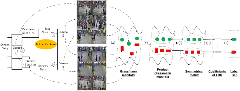
Figure 1: An overview of our proposed LRR on Product Grassmann manifolds for multi-camera videos clustering. (a) The multi-camera videos are represented as Grassmann points. (b) The Grassmann points from same class are represented as a Product Grassmann point. (c) The Grassmann points are mapped onto symmetrical matrices. (d) The Product Grassmann points are represented by LRR on PGM. (e) Clustering by NCut.

To address these problems, many methods have been proposed to joint videos collected from different cameras and use them in human detection, tracking, and recognition. For human detection, there has been considerable improvement in multi-camera methods compared to single-camera methods [7, 8, 9, 10]. This improvement obviously comes from the fact that an observed human/object in a multi-camera system may appear in different views simultaneously or at different times depending on the overlaps between camera views. Using these multi-information, one can detect objects from each camera’s view or combine these information to form a common view for detection. Similarly, the common view can be used for tracking targets using sequential belief propagation [11, 12, 13], where one usually assumes that the topology of camera views is known. Many human action recognition methods are based on human action trajectories extracted from multiple cameras [14, 15] and use the combined trajectories of an object observed in different camera views for activity analysis with the similar approaches developed from single-camera systems. Although these methods can process the dramatic changes in speed and direction of actions, the requirement of accurate tracking trajectories is also challenging. Other approaches like [16, 17] model as a bag of visual words in each camera view for representing actions, instead of using any tracking information. However this feature representation is sensitive to view changes, and some high level features have to be shared across camera views.

Most multi-camera methods achieve better performance than single-camera methods in many scenarios, yet there still exist some obstacles that need to be conquered. One important issue is how to properly represent the action data captured by multiple cameras, although there are some methods, usually developed for specific applications. The other is how to effectively fuse or combine the information from different cameras as an overall entity. Majority of existing methods constructs a common map from multiple cameras, which can be fed into any single-camera methods. However this type of strategies can only be regarded as a naïve fusion of multi-camera videos without considering latent relations.

In this paper, we investigate a new way of data representation for multi-camera systems, thus further explore fusion methods for data captured by multiple cameras. The traditional video features, such as the image bag [18] , Local Binary Patterns from Three Orthogonal Plans (LBP-TOP) [19] and Improved Dense Trajectories (IDT) [20] are measured in terms of Euclidean distance. In fact, it has been proved that many high-dimensional data in computer vision tasks are actually embedded in low dimensional manifolds. Using Euclidean geometry is inappropriate in most of such cases, so, to get a proper data representation, it is critical to reveal the nonlinear manifold structure underlying these high-dimensional video data.

The classic manifold learning methods are proposed to learn or find nonlinear properties, such as Locally Linear Embedding (LLE) [21], ISOMAP [22], and Locally Linear Projection (LLP) [23]. But these methods only depend on data samples and the manifold underlying the data is unknown. Different from learning nonlinear manifold structure from data, in many scenarios, data are generated from a known manifold. For example, in image analysis, covariance matrices are used to describe region features [24]. A covariance matrix is actually a point on the manifold of symmetric positive definite matrices. Similarly, an image set can be represented as a point on the so-called Grassmann manifold in terms of subspace representation [25].

For the high dimensional video data, to incorporate the possible non-linear intrinsic property, we propose a manifold representation, in which a video is represented as a point on Grassmann manifold. To further fuse the multiple videos, we propose to extend Grassmann manifolds to their product space and obtain a fused representation for multi-camera data, named the Product Grassmann manifold. This is motivated by the fact that product space is good at representing multi-factors determined by multi-subspaces.

To verify the performance of the product manifold representation for multi-camera data, we select human activity clustering in multi-camera surveillance for evaluation. The reason to select clustering tasks is that the clustering problem, especially the video scene clustering, is a challenging problem in computer vision, pattern recognition and signal processing [26, 27, 28]. Concretely, we consider the subspace clustering method in our paper. Particularly, the prospective subspace clustering method, the spectral clustering methods based on affinity matrix, is adopted here.

The main component of the spectral clustering methods is to construct a proper affinity matrix for a dataset and then the affinity matrix is implemented by any clustering algorithms to obtain the final clustering results, such as K-means and Normalized Cuts (NCut) [29]. There are two classical spectral clustering methods: Sparse Subspace Clustering (SSC) [26] and low rank representation (LRR) [30, 31]. The SSC method assumes that the data of subspaces are independent and are sparsely represented under the so-called $\ell_{1}$ Subspace Detection Property [32], in which the within-class affinities are sparse and the between-class affinities are all zeros. It has been proved that under certain conditions the multiple subspace structures can be exactly recovered via $\ell_{p}(p\leq 1)$ minimization [33]. Different from the independent sparse representation for data objects in SSC, the LRR method introduces a holistic constraint, i.e., the low rank or nuclear norm $\|\cdot\|_{*}$ to reveal the latent structural sparse property embedded in the dataset. It has been proven that, when the high-dimensional dataset is actually from a union of several low dimension subspaces, the LRR method can reveal this structure through subspace clustering [31].

Although the subspace clustering methods have good performance in many applications, the current methods assume that data objects come from linear space and the similarity among data is measured in Euclidean-alike distance. For the manifold representation of multi-camera videos, the clustering methods should be implemented on the manifold. Therefore, we explore the geometry property of the Product Grassmann manifold and extend the conventional LRR method onto Product Grassmann manifold, namely PGLRR model. Furthermore, to capture the local structure of data, we introduce Laplacian constraint to the proposed LRR model on Product Grammann manifold, namely LapPGLRR.

The main idea and framework of the proposed human activity clustering in multi-camera video surveillance based on Laplacian LRR on the product Grassmann manifold is illustrated in Fig. 1. The contributions of this work are

• Proposing a new data representation based on the Product Grassmann manifold for multi-camera video data;

• Formulating the LRR model on the Product Grassmann Manifold and providing a practical and effective algorithm for the proposed PGLRR model; and

• Introducing the Laplacian constraint for LRR model on the Product Grassmann manifold.

The rest of the paper is organized as follows. In Section 2, we review the property of Grassmann manifold and briefly describe the conventional LRR method. In Section 3, we propose the Product Grassmann Manifold data representation for multi-camera video data and present the LRR model on the Product Grassmann Manifold (PGLRR) for clustering. In Section 4, we give the solutions to PGLRR and LapPGLRR in detail. In Section 5, the performance of the proposed method is evaluated on clustering problems with several public databases. Finally, the conclusion and the future work are discussed in Section 6.

2 Preliminaries

2.1 Grassmann Manifold

Grassmann manifold $\mathcal{G}(p,d)$ [34] is the space of all $p$-dimensional linear subspaces of $\mathbb{R}^{d}$ for $0\leq p\leq d$. A point on Grassmann manifold is a $p$-dimensional subspace of $\mathbb{R}^{d}$ which can be represented by any orthonormal basis $X=[\mathbf{x}_{1},\mathbf{x}_{2},...,\mathbf{x}_{p}]\in\mathbb{R}^{d\times p}$. The chosen orthonormal basis is called a representative of its subspace $\text{span}(X)$. Grassmann manifold is an abstract quotient manifold. There are many ways to represent Grassmann manifold. In this paper, we take the way of embedding Grassmann manifold into the space of symmetric matrices $\text{Sym}(d)$.

For convenience, in the sequel we use the same symbol $X$ of the representative orthonormal basis to represent the subspace $\text{span}(X)$. The embedding representation of Grassmann manifold is given by the following mapping [25]:

$$\Pi:\mathcal{G}(p,d)\rightarrow\text{Sym}(d),\ \ \ \Pi(X)=XX^{T}.$$ (1)

The embedding $\Pi$ is diffeomorphism [35] (a one-to-one, continuous, differentiable mapping with a continuous, differentiable inverse). Given this property, a distance on Grassmann manifold can be induced by the following formula defined by the squared Frobenius norm. Hence it is reasonable to replace the distance on Grassmann manifold with the following distance defined on the symmetric matrix space under this mapping,

$$d^{2}_{g}(X,Y)=\frac{1}{2}\|\Pi(X)-\Pi(Y)\|^{2}_{F}.$$ (2)

2.2 Product Grassmann Manifold (PGM)

The PGM is defined as a space of product of multiple Grassmann manifolds, denoted by $\mathcal{PG}_{d:p_{1},...,p_{M}}$. For a given set of natural number $\{p_{1},...,p_{M}\}$, we define the PGM $\mathcal{PG}_{d:p_{1},...,p_{M}}$ as the space of $\mathcal{G}(p_{1},d)\times\cdot\cdot\cdot\times\mathcal{G}(p_{M},d)$. So a PGM point can be represented as a collection of Grassmannian points, denoted by $[X]=\{{X}^{1},...,{X}^{M}\}$ such that $X^{m}\in\mathcal{G}(p_{m},d),m=1,...,M$.

For our purpose, we consider a weighted sum of Grassmann distances as the distance on PGM,

$$d_{\mathcal{PG}}([X],[Y])^{2}=\sum_{m=1}^{M}w_{m}d_{g}^{2}(X^{m},Y^{m}),$$ (3)

where $w_{m}$ is the weight to represent the importance of the $m$-th Grassmann space. In practice, it can be determined by a data driven manner or according to prior knowledge. In this paper, we simply set all $w_{m}=1$. So from (2), we simply deduce the following distance on PGM,

$$d_{\mathcal{PG}}([X],[Y])^{2}=\sum\limits_{m=1}^{M}\frac{1}{2}\|X^{m}(X^{m})^{T}-Y^{m}(Y^{m})^{T}\|_{F}^{2}.$$ (4)

2.3 Low Rank Representation (LRR) [30]

Given a set of data drawn from an unknown union of subspaces $\mathbf{X}=[\mathbf{x}_{1},\mathbf{x}_{2},...,\mathbf{x}_{N}]\in\mathbb{R}^{D\times N}$ where $D$ is the data dimension, the objective of subspace clustering is to assign each data sample to its underlying subspace. The basic assumption is that the data in $\mathbf{X}$ are drawn from a collection of $K$ subspaces $\{\mathcal{S}_{k}\}^{K}_{k=1}$ of dimensions $\{d_{k}\}^{K}_{k=1}$.

According to the principle of self representation of data, each data point from a dataset can be written as a linear combination of the remaining data points, i.e., $\mathbf{X}=\mathbf{X}\mathbf{Z}$, where $\mathbf{Z}\in\mathbb{R}^{N\times N}$ is the coefficient matrix of similarity.

The LRR model is formulated as

$$\min_{\mathbf{Z},\mathbf{E}}\|\mathbf{E}\|^{2}_{F}+\lambda\|\mathbf{Z}\|_{*},\text{ s.t. }\mathbf{X}=\mathbf{X}\mathbf{Z}+\mathbf{E},$$ (5)

where $\mathbf{E}$ is the error resulting from the self-representation. Similar to the original LRR model, the Frobenius norm can be replaced by the Euclidean $\ell_{2,1}$-norms. LRR takes a holistic view in favor of a coefficient matrix in the lowest rank, measured by the nuclear norm $\|\cdot\|_{*}$.

3 PGM representation of Multi-Camera video Data and Laplacian LRR Clustering on PGM

In this section, we first describe the novel representation of the multi-camera video data by PGM and then extend the standard LRR model onto this manifold to obtain a new LRR model on PGM. We also integrate the Laplacian constraint, which captures the local structure of the points on PGM, with the LRR model on PGM to construct a Laplacian LRR model on PGM. Based on the Laplacian LRR model on PGM, we realize the clustering of the multi-camera videos by spectral clustering methods.

3.1 PGM representation of Multi-Camera video Data

We denote the multi-camera human action video samples by $\mathcal{Y}=\{[Y_{1}],...,[Y_{N}]\}$, where $N$ is the number of samples and each sample $[Y_{i}]$ represents a video set which consists of $M$ video clips of an action captured by $M$ cameras simultaneously, denoted by $[Y_{i}]=\{C^{1}_{i},...,C_{i}^{M}\}$.

For each video clip $C^{m}_{i},m=1,...,M$ in the $i$-th sample $[Y_{i}]$, we select all the frames from the clip to form an image set as its delegate, denoted by $\mathbf{S}_{i}^{m},m=1,...,M$. According to [36], this image set can be represented as a Grassmannian point by using an orthogonal basis of the subspace generated by $\mathbf{S}_{i}^{m}$. Here we adopt the SVD to construct an orthogonal basis, the so-called a Grassmannian point, to represent this video clip, see [36, 37] for more details. For our purpose in this paper, we give a brief description. Firstly, we vectorize all frames in $\mathbf{S}_{i}^{m}$ and align these vectors as a matrix. For convenience, we still use $\mathbf{S}_{i}^{m}$ to denote the matrix. Under the SVD of $\mathbf{S}_{i}^{m}$, we construct a $p_{m}$-dimension subspace from the first $p_{m}$ singular vectors. This $p_{m}$-dimension subspace can be used to approximate the column space of $\mathbf{S}_{i}^{m}$. That is, if $\mathbf{S}_{i}^{m}=U_{i}^{m}\Sigma_{i}^{m}V_{i}^{m}$ is the SVD, then $X^{m}_{i}=U_{i}^{m}(:,1:p_{m})\in\mathcal{G}(p_{m},d)$. $p_{m}$ could be determined by retaining e.g. $90\%$ of the accumulative eigenvalues of $\Sigma_{i}^{m}$.

Combining the $M$ Grassmannian points of the $i$-th sample $[Y_{i}]$, we obtain the aforementioned Product Grassmann representation of $[Y_{i}]$, denoted by $[X_{i}]=\{X^{1}_{i},...,X^{M}_{i}\}\in\mathcal{PG}_{d:p_{1},..,p_{M}}$. By this way, we finally get the PGM representation of the multi-camera human action video samples $\mathcal{Y}=\{[Y_{1}],...,[Y_{N}]\}$, denoted by $\mathcal{X}^{0}=\{[X_{1}],[X_{2}],...,[X_{N}]\}$. Next, we will discuss the clustering problem on PGM, i.e. clustering PGM points $[X_{i}],i=1,...,N$ in $\mathcal{X}^{0}$ into their proper classes.

3.2 LRR on the Product Grassmann Manifolds

To generalize the LRR model (5) onto PGM and implement clustering on the dataset $\mathcal{X}^{0}$, we first note that in (5)

$$\|\mathbf{E}\|^{2}_{F}=\|\mathbf{X}-\mathbf{X}\mathbf{Z}\|^{2}_{F}=\sum_{i=1}^{N}\|\mathbf{x}_{i}-\sum_{j=1}^{N}\mathbf{z}_{ij}\mathbf{x}_{j}\|^{2},$$

where the measure $\|\mathbf{x}_{i}-\sum_{j=1}^{N}\mathbf{z}_{ij}\mathbf{x}_{j}\|$ is the Euclidean distance between the point $\mathbf{x}_{i}$ and its linear combination of all data points including $\mathbf{x}_{i}$. Accordingly on PGM we simulate this operation and propose the following form of LRR,

$$\begin{aligned} &\min_{Z}\sum^{N}_{i=1}\bigg{\|}[X_{i}]\ominus(\biguplus^{N}_{j=1}\mathbf{z}_{ij}\odot[X_{j}])\bigg{\|}_{\mathcal{PG}}+\lambda\|\mathbf{Z}\|_{*},\\ \end{aligned}$$ (6)

where $\left\|[X_{i}]\ominus(\biguplus^{N}_{j=1}\mathbf{z}_{ij}\odot[X_{j}])\right\|_{\mathcal{PG}}$ with the operator $\ominus$ represents the manifold distance between $[X_{i}]$ and its “linear” reconstruction $\biguplus^{N}_{j=1}\mathbf{z}_{ij}\odot[X_{j}]$. Here the combination operators are abstract at this stage. To get a concrete LRR model on PGM, one needs to define a proper distance and proper combination operations on the manifold.

From the geometric property of the Grassmann manifold, we can use the metric of the Grassmann manifold and the PGM in (2) and (3) to replace the manifold distance in (6), i.e.

$$\left\|[X_{i}]\ominus(\biguplus^{N}_{j=1}\mathbf{z}_{ij}\odot[X_{j}])\right\|_{\mathcal{PG}}=d_{\mathcal{PG}}([X_{i}],\biguplus^{N}_{j=1}\mathbf{z}_{ij}\odot[X_{j}]).$$

In addition, from (1) we know that the embedded points in the space of $Sym(d)$ are semi-positive definite matrices. With any positive coefficients, the linear combination on $Sym(d)$ is closed. Thus it is natural to define the “linearly” reconstructed Grassmannian point $\biguplus^{N}_{j=1}\mathbf{z}_{ij}\odot[X_{j}]$ as follows,

$$\Pi\left(\biguplus^{N}_{j=1}\mathbf{z}_{ij}\odot[X_{j}]\right):=\mathcal{X}\times_{4}\mathbf{z}_{i},$$

where $\mathbf{z}_{i}$ is the $i$-th column of matrix $\mathbf{Z}$ and $\mathcal{X}=\{\mathcal{X}_{1},\mathcal{X}_{2},...,\mathcal{X}_{N}\}$ is a $4$-th order tensor such that the $4$-th order slices are the $3$rd order tensors $\mathcal{X}_{i}$, and each $\mathcal{X}_{i}$ is constructed by stacking the symmetrically mapped matrices along the 3rd mode. Its mathematical representation is given by

$\mathcal{X}_{i}=\{X_{i}^{1}(X_{i}^{1})^{T},X_{i}^{2}(X_{i}^{2})^{T},...,X_{i}^{M}(X_{i}^{M})^{T}\}\subset\text{Sym}(d)$. And $\times_{4}$ means the mode-4 multiplication of a tensor and a vector (and/or a matrix) [38].

Finally, we can construct the LRR model on the PGM followed as [38]

$$\min\limits_{\mathbf{E},\mathbf{Z}}\|\mathbf{Z}\|_{*}+\lambda\|\mathbf{E}\|_{F}^{2}\ \ \ \text{s.t.}\ \ \ \mathcal{X}=\mathcal{X}\times_{4}\mathbf{Z}+\mathbf{E}.$$ (7)

In other words, the LRR on PGM is implemented on the product of the symmetric matrix spaces.

3.3 Laplacian LRR on The Product Grassmann Manifolds

The low rank term in the LRR model (7) on PGM makes a holistic constraint on the coefficient matrix $\mathbf{Z}$. However, the points on PGM also have their geometric property in sense of geodesic distance on the manifold. So this geometric property should also be converted to their corresponding LRR representation coefficient matrix $\mathbf{Z}$. From this observation, we further add a geometric constraint on the coefficient matrix $\mathbf{Z}$ in terms of Laplacian Matrix to get the following Laplacian LRR on the Product Grassmann Manifolds.

For the coefficient matrix $\mathbf{Z}$, we consider imposing the local geometrical structures to enforce the coefficient matrix preserving the intrinsic structures of original data on the manifold. Under the LRR model, $\mathbf{z}_{i}$ and $\mathbf{z}_{j}$ are the new representations of data objects $\mathbf{x}_{i}$ and $\mathbf{x}_{j}$, respectively. The distance between $\mathbf{z}_{i}$ and $\mathbf{z}_{j}$ defines certain similarity between data $\mathbf{x}_{i}$ and $\mathbf{x}_{j}$. Laplacian regularization is considered as a good way to preserve the similarity. As a result, we add the Laplacian regularization into the objective function (7) as follows,

$$\min\limits_{\mathbf{Z},\mathbf{E}}\|\mathbf{Z}\|_{*}+\lambda\|\mathbf{E}\|_{F}^{2}+\beta\sum\limits_{i,j}\|\mathbf{z}_{i}-\mathbf{z}_{j}\|_{2}^{2}w_{ij}$$ (8)

$$\text{s.t.}\ \ \mathcal{X}=\mathcal{X}_{\times_{4}}\mathbf{Z}+\mathbf{E}$$

where $w_{ij}$ is the geodesic distance between the Product Grassmannian points $[X_{i}]$ and $[X_{j}]$. The simplified form of the $3$rd term in (8) is given by

$$\sum\limits_{i,j}\|\mathbf{z}_{i}-\mathbf{z}_{j}\|_{2}^{2}w_{ij}=2\text{tr}(\mathbf{Z}^{T}L\mathbf{Z}),$$ (9)

where $L=D-W$ and $D$ is the diagonal matrix with diagonal elements $d_{ii}=\sum\limits_{j}w_{ij}$. The element $w_{ij}$ is defined by the geodesic distance, refer to (4)

$$w_{ij}=d_{\mathcal{PG}}([X_{i}],[X_{j}])=\sqrt{\sum^{M}_{m=1}d^{2}_{g}(X^{m}_{i},X^{m}_{j})}.$$

Thus, the objective function (8) can be rewritten as,

$$\min\limits_{\mathbf{E},\mathbf{Z}}\|\mathbf{Z}\|_{*}+\lambda\|\mathbf{E}\|_{F}^{2}+2\beta\text{tr}(\mathbf{Z}L\mathbf{Z}^{T}),\$$ (10)

$$\text{s.t.}\ \ \mathcal{X}=\mathcal{X}_{\times_{4}}\mathbf{Z}+\mathbf{E}.$$

For convenience,we abbreviate it by LapPGLRR.

3.4 Clustering algorithm for the multi-camera videos by the Laplacian LRR on PGM

For the multi-camera videos $\mathcal{Y}=\{[Y_{1}],...,[Y_{N}]\}$, we first find out their PGM representation $\mathcal{X}^{0}=\{[X_{1}],...,[X_{N}]\}$ as described in Section 3.1. After formulating the PGLRR model in (7) or LapPGLRR model in (10) and solving these optimization problems (How to solve these problems will be discussed in the next Section.), we can find the data representation coefficient matrix $\mathbf{Z}$. Under the data self-representative principle used in the models, the element $\mathbf{z}_{ij}\in\mathbf{Z}$ represents the similarity between data $i$ and $j$. So a natural way is to define the affinity matrix $\hat{\mathbf{Z}}=(|\mathbf{Z}|+|\mathbf{Z}^{T}|)/2$ for model (7) or (10). This affinity matrix $\hat{\mathbf{Z}}$ can be performed on any spectral clustering algorithms, such as Ncut [29], to obtain the final clustering result. The whole clustering procedure of the proposed clustering algorithm for multi-camera videos by the Laplacian LRR on PGM is summarized as Algorithm 1.

Algorithm 1 Clustering algorithm for multi-camera videos by the Laplacian LRR on PGM

0:  The multi-camera videos for clustering $\mathcal{Y}$.

0:  The clustering results of $\mathcal{Y}$.

1:  Representing $\mathcal{Y}$ as PGM pionts $\mathcal{X}^{0}$ as Section 3.1;

2:  Calculating geodesic distance $w_{ij}$ between $[X_{i}]$ and $[X_{j}]$ and constructing the Laplace matrix $L$;

3:  Obtaining the LRR representation $\mathbf{Z}$ of $\mathcal{X}$ by (10) ;

4:  Computing the affinity matrix $\hat{\mathbf{Z}}=(|\mathbf{Z}|+|\mathbf{Z}^{T}|)/2$;

5:  Implementing NCut$(\hat{\mathbf{Z}})$ to get the final clustering result of $\mathcal{Y}$.

4 Solution to Laplacian LRR on PGM

First, we give the solution to the LRR on PGM in (7) in which only the holistic low rank constraint is considered. Then the solution to the LaplacianLRR on PGM in (10) is discussed.

4.1 Solution to LRR on PGM

To avoid tedious calculation between the $4$-order tensor and the matrix in (7), we briefly analyze the representation of the reconstruction tensor error $\mathbf{E}$ and translate the optimization problem into an equivalent and solvable optimization model.

The explicit form of $\|\textbf{E}\|_{F}^{2}$ is given by

$$\|\mathbf{E}\|_{F}^{2} =\sum^{N}_{i=1}\sum^{M}_{m=1}\|(X_{i}^{m}(X_{i}^{m})^{T}-\sum\limits_{j=1}^{N}\mathbf{z}_{ij}(X_{j}^{m}(X_{j}^{m})^{T}))\|_{F}^{2}.$$

To simplify the expression for $\|\mathbf{E}\|_{F}^{2}$, we firstly note that the matrix property

$$\|A\|_{F}^{2}=\text{tr}(A^{T}A)$$

and denote

$$\Delta_{ij}^{m}=\text{tr}[((X_{j}^{m})^{T}X_{i}^{m})((X_{i}^{m})^{T}X_{j}^{m})].$$ (11)

Observing that $\Delta_{ij}^{m}=\Delta_{ji}^{m}$, we define $M$ $N\times N$ symmetric matrices as

$$\Delta^{m}=(\Delta_{ij}^{m})_{i=1,j=1}^{N},\ \ \ m=1,2,...,M.$$ (12)

Moreover, it is easy to prove that

$$\|\mathbf{E}\|_{F}^{2}=-2\text{tr}(\mathbf{Z}\Delta)+\text{tr}(\mathbf{Z}\Delta\mathbf{Z}^{T})+\text{const},$$ (13)

where $\Delta=\sum_{m=1}^{M}\Delta^{m}$ and the term const collects all the terms irrelevant to the variable $\mathbf{Z}$.

Similar to [36], it is easy to prove that $\Delta$ is positive semi-definite. Consequently, we have a spectral decomposition of $\Delta$ given by

$$\Delta=UDU^{T},$$

where $U^{T}U=I$ and $D=\text{diag}(\sigma_{i})$ with non-negative eigenvalues $\sigma_{i}$. So (13) becomes

$$\|\mathbf{E}\|_{F}^{2}=\|\mathbf{Z}\Delta^{\frac{1}{2}}-\Delta^{\frac{1}{2}}\|_{F}^{2}+\text{const},$$

after variable elimination and problem (7) can be converted to

$$\min\limits_{\mathbf{Z}}\|\mathbf{Z}\Delta^{\frac{1}{2}}-\Delta^{\frac{1}{2}}\|_{F}^{2}+\lambda\|\mathbf{Z}\|_{*}.$$ (14)

There exists a closed form solution to the optimization problem (14) following [39], and it is given by the following theorem.

Theorem 1.

Given that $\Delta=UDU^{T}$ as defined above, the solution to (14) is given by

$$\mathbf{Z}^{*}=UD_{\lambda}U^{T},$$

where $D_{\lambda}$ is a diagonal matrix with its $i$-th element defined by

$$D_{\lambda}(i,i)=\begin{cases}1-\frac{\lambda}{\sigma_{i}}&\text{ if }\sigma_{i}>\lambda,\\ 0&\text{ otherwise}.\end{cases}$$

4.2 Solution to Laplacian LRR on PGM

By using the same technique deriving the above PGLRR algorithm, it is easy to deduce the equivalent form of the model in (10) as follows,

$$\min\limits_{\mathbf{Z}}-2\lambda\text{tr}(\mathbf{Z}\Delta)+\lambda\text{tr}(\mathbf{Z}\Delta\mathbf{Z}^{T})+2\beta\text{tr}(\mathbf{Z}L\mathbf{Z}^{T})+\|\mathbf{Z}\|_{*}.$$ (15)

We employ the Augmented Lagrangian Multiplier (ALM) to solve this problem. So we let $J=\mathbf{Z}$ to separate the variable Z from different terms. Then problem (15) can be formulated as follows,

$$\min\limits_{\mathbf{Z},J}-2\lambda\text{tr}(\mathbf{Z}\Delta)+\lambda\text{tr}(\mathbf{Z}\Delta\mathbf{Z}^{T})+2\beta\text{tr}(\mathbf{Z}L\mathbf{Z}^{T})+\|J\|_{*}$$ (16)

$$\text{s.t.}\ \ J=\mathbf{Z}$$

Its Augmented Lagrangian Multiplier formulation can be defined as the following unconstrained optimization,

$$-2\lambda\text{tr}(\mathbf{Z}\Delta)+\lambda\text{tr}(\mathbf{Z}\Delta\mathbf{Z}^{T})+2\beta\text{tr}(\mathbf{Z}L\mathbf{Z}^{T})+\|J\|_{*}$$ (17)

$$+\langle A,\mathbf{Z}-J\rangle+\frac{\mu}{2}\|\mathbf{Z}-J\|_{F}^{2}$$

where $A$ is the Lagrangian Multiplier and $\mu$ is a weight to tune the error term of $\|\mathbf{Z}-J\|_{F}^{2}$.

Now, the above problem can be solved by solving the following two subproblems in an alternative manner, fixing $\mathbf{Z}$ or $J$ to optimize the other, respectively.

When fixing $\mathbf{Z}$, the following subproblem is solved to update $J$

$$\min\limits_{J}\|J\|_{*}+\langle A,\mathbf{Z}-J\rangle+\frac{\mu}{2}\|\mathbf{Z}-J\|_{F}^{2}$$ (18)

When fixing $J$, the following subproblem is solved to update $\mathbf{Z}$

$$\min\limits_{\mathbf{Z}} -2\lambda\text{tr}(\mathbf{Z}\Delta)+\lambda\text{tr}(\mathbf{Z}\Delta\mathbf{Z}^{T})+2\beta\text{tr}(\mathbf{Z}L\mathbf{Z}^{T})$$ (19)

$$+\langle A,\mathbf{Z}-J\rangle+\frac{\mu}{2}\|\mathbf{Z}-J\|_{F}^{2}$$

Subproblem (18) can be solved by the following way. Firstly, the optimization is revised as follows,

$$\begin{split}\min\limits_{J}(||J||_{*}+\frac{\mu}{2}||J-(\mathbf{Z}+\frac{A}{\mu})||_{F}^{2}).\end{split}$$ (20)

(20) has a closed-form solution given by,

$$J^{*}=\Theta_{\mu^{-1}}(\mathbf{Z}+\frac{A}{\mu}),$$

where $\Theta(\cdot)$ denotes the singular value thresholding operator (SVT), see [40].

The subproblem in (19) is a quadratic optimization problem with respect to $\mathbf{Z}$. The closed-form solution is given by

$$\mathbf{Z}=(2\lambda\Delta+\mu J-A)(2\lambda\Delta+2\beta L+\lambda I)^{-1}$$ (21)

Solving the above two subproblems alternatively results in the complete solution to LapPGLRR. The whole procedure of LapPGLRR through solving problem (15) is summarized in Algorithm 2.

Algorithm 2 Solving Problem (15) by ALM.

0:  The Product Grassmann sample set $\{[X_{i}]\}_{i=1}^{N}$, $[X_{i}]\in\mathcal{PG}_{n:p_{1},..,p_{M}}$, and the balancing parameters $\lambda$ and $\beta$.

0:  The Low-Rank Representation $Z$   

1:  Initialize:$J=Z=0,A=0,\mu=10^{-6},\mu_{max}=10^{10}$ and $\varepsilon=10^{-8}$

2:  for m=1:M do

3:     for i=1:N do

4:        for j=1:N do

5:           $\Delta_{ij}^{m}\leftarrow\mbox{tr}[({X_{j}^{m}}^{T}X_{i}^{m})({X_{i}^{m}}^{T}X_{j}^{m})]$;

6:        end for

7:     end for

8:  end for

9:  for m=1:M do

10:     $\Delta\leftarrow\Delta+\Delta^{m}_{::}$;

11:  end for

12:  while not converged do

13:     fix $Z$ and update $J$ by $J\leftarrow\min\limits_{J}(||J||_{*}+\langle A,Z-J\rangle+\frac{\mu}{2}||Z-J||_{F}^{2})$;

14:     fix $J$ and update $Z$ by $Z=(2\lambda\Delta+\mu J-A)(2\lambda\Delta+2\beta L+\lambda I)^{-1}$ ;

15:     update the multipliers: $A\leftarrow A+\mu(Z-J)$

16:     update the parameter $\mu$ by $\mu\leftarrow\min(\rho\mu,\mu_{\mbox{max}})$

17:     check the convergence condition: $\|Z-J\|_{\infty}<\varepsilon$

18:  end while

5 Experiments

In this section, we evaluate the performance of our proposed clustering approaches on a human activity multi-camera video dataset we collected, the Dongzhimen Transport Hub Crowd Dataset; and other two multi-view or multi-modality individual action datasets, the ACT42 action dataset and the SKIG action clips dataset. The experiments are conducted on these three datasets with four state-of-the-art manifold-based clustering methods and three classic clustering methods using both LBP-TOP video features [19] and IDT video features [20]. The IDT video feature is one of the state-of-the-art effective representations for action recognition in videos. For a summary, we list all the comparing methods as follows:

• GLRR-F [36]: Low Rank Representation on Grassmann Manifold embeds the image sets into the Grassmann manifold and extends the standard LRR model onto the Grassmann manifold.

• SCGSM [41]: Statistical computations on the Grassmann and Stiefel manifolds uses a statistical model derived from Riemannian geometry of the manifold.

• SMCE [42]: Sparse Manifold Clustering and the Embedding utilizes the local manifold structure to find a small neighborhood around each data point and connects each point to its neighbours with appropriate weights.

• LS3C [43]: Latent Space Sparse Subspace Clustering learns the projection of data and finds the sparse coefficients in the low-dimensional latent space.

• LRR+IDT/LBP-TOP: The standard LRR method [30] is implemented with the IDT features or LBP-TOP features of videos instead of the raw data.

• K-means+IDT/LBP-TOP: K-means algorithm is implemented on the IDT features or LBP-TOP features of videos.

• SPC+IDT/LBP-TOP: Spectral Clustering method [44] is implemented on the IDT features or LBP-TOP features of videos.

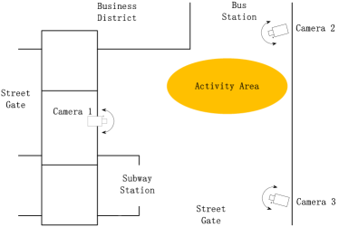
Figure 2: An illustrative example for the positions of three cameras in Dongzhimen Transport Hub.

In all the above methods, Grassmann manifold representation, IDT video features and LBP-TOP video features are extracted from videos. In IDT, one firstly learns a codebook from a set of motion trajectory features constructed by several descriptors (i.e., Trajectory, HOG, HOF and MBF). However, at the next encoding stage, some information may be lost when a trajectory feature is represented by the nearest visual word in codebook. LBP-TOP describes videos using three Histograms of Spatial-temporal LBP features, which captures local spatial and temporal information at pixel level but fails to retain the global structure relation when computing the histograms. Grassmann manifold representation is generated by selecting the first $p$ singular vectors according to the descending eigenvalues in SVD, which can preserve the principal information of videos. Through the following experiments, we will prove the advantages of using Grassmann manifold representation.

Our proposed method PGLRR consists of three main ingredients: Product manifold, Grassmann manifold representation and LRR. In the following experiments, we intend to find out which one of them plays a key role in boosting clustering accuracy. We take three compared methods, GLRR-F, SCGSM and LRR+IDT/LBP-TOP, as the most important baselines. PGLRR extends GLRR-F onto product manifold, thus comparing the performance of PGLRR with GLRR-F will demonstrate the importance of product manifold. To evaluate the importance of Grassmann manifold representation, we compare PGLRR’s performance to SCGSM’s without LRR. Similarly, for assessing the impact of LRR, we can compare PGLRR’s performance to LRR+IDT/LBP-TOP’s without Grassmann manifold representation. We conclude that all three ingredients improve the effectiveness of PGLRR, respectively, as demonstrated in the following experiments.

5.1 Experimental Datasets

1) Dongzhimen Transport Hub Crowd Dataset (DTHC)

We construct a multi-camera human activity dataset to evaluate the proposed methods. We choose the Dongzhimen Transport Hub in Beijing, China, as a site to collect multi-camera data. Dongzhimen Transport Hub is one of the busiest transport hubs in Beijing. Many passengers take transfer between different routes in this hub everyday, hence there exist complicated crowd activities. We deploy three cameras in a hall (as shown in Fig. 2) to capture the videos of passengers. The dataset is captured from 06:00 to 22:00 on a Saturday. We pick up 182 multi-camera samples as our experimental data. Each sample has three video clips. Samples of this dataset are labeled with three level of crowd actions: heavy, light, and medium. There are 48 samples of heavy level, 76 samples of light level and 58 samples of medium level. The frames are converted to gray images and each image is normalized to size $32\times 58$. Some samples of the Dongzhimen Transport Hub Crowd dataset are shown in Fig. 3.

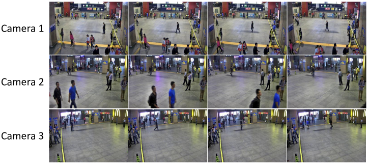
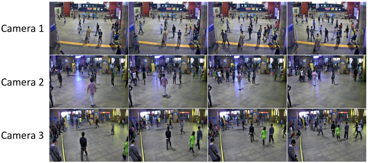
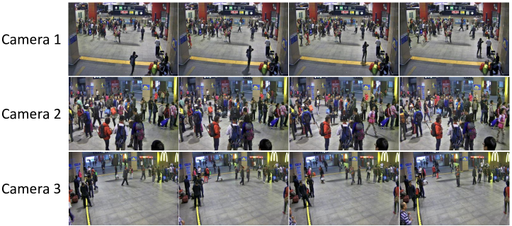
Figure 3: Some samples of three crowd actions in Dongzhimen Transport Hub Crowd dataset. Each row shows frames captured by one of the three cameras. (a) light level. (b) medium level. (c) heavy level.

2) ACT 42 Human Action Dataset

This dataset consists of 14 complex action patterns performed by 21 subjects, collected from four cameras in different viewpoints. Each type of action is repeated twice by each subject. These 14 actions are: “Collapse”, “Stumble”, “Drink”, “Make phone”, “Read Book”, “Mop Floor”, “Pick up”, “Throw away”, “Put on”, “Take off”, “Sit on”, “Sit down”, “Twist open”, and “Wipe clean”. Each clip contains 35 to 554 frames. To reduce the computation cost and the memory requirement of all the methods, each image is resized from $480\times 640$ pixels to $32\times 48$. Some frame samples of the ACT 42 dataset are shown in Fig. 4.

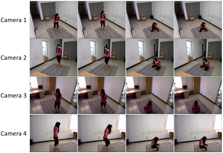
Figure 4: Some samples in The ACT42 samples. Each row presents a video sequence form a camera. There are 4 cameras to record the same action simultaneously.

3) SKIG Action Dataset

This dataset contains 1080 RGB-D sequences captured by a Kinect sensor. This dataset stores ten kind of gestures of six persons: ’circle’, ’triangle’, ’up-down’, ’right-left’, ’wave’, ’Z’, ’cross’, ’come-here’, ’turn-around’, and ’pat’. All the gestures are performed by fist, finger and elbow respectively under three backgrounds (wooden board, white plain paper and paper with characters) and two illuminations (strong light and poor light). Each RGB-D sequence contains 63 to 605 frames. Here the images are normalized to $24\times 32$ with mean zero and unit variance. Fig. 5 shows some RGB and DEPTH images.

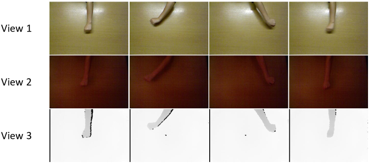
Figure 5: Some samples with different viewpoints and illuminations in SKIG dataset. View 1 represents light sequences, View 2 represents dark sequences and View 3 represents depth sequences.

5.2 Experimental Parameters

In our experiments, some model parameters in the proposed methods should be adequately adjusted , such as $\lambda$, $\beta$ and $\varepsilon$. To assess the impact of these model parameters, we will conduct experiments by varying one parameter while keeping others fixed to achieve the best parameter values.

$\lambda$ and $\beta$ are the most important penalty parameters for balancing the error term, the low-rank term and Laplacian regularization term in our proposed methods. Empirically, the best value of $\lambda$ depends on particular applications and has to be chosen from a large range of values to get a better performance. From our experiments, we have observed that when the cluster number is increasing, the best $\lambda$ is decreasing. Additionally, $\lambda$ will be smaller when the noise level in data is lower while $\lambda$ will become larger if the noise level higher. These observations are useful in selecting a proper $\lambda$ value for different datasets. However, the value of $\beta$ is usually very small for various applications with range from $1.0\times 10^{-4}$ to $1.0\times 10^{-2}$. But it does not mean this parameter is unimportant, because the element values of $Z$ is usually thousand smaller than the element values of Laplacian matrix $L$.

The error tolerance $\varepsilon$ is also an important parameter in controlling the terminal condition, which bounds the allowed reconstructed error. We experimentally seek a proper value of $\varepsilon$ to make the iteration process stop at an appropriate level of reconstructed error. Here we set $\varepsilon=1.0\times 10^{-8}$ for all experiments.

The performances of different algorithms are measured by the following clustering accuracy

$$\text{Accuracy}=\frac{\text{number of correctly classified points}}{\text{total number of points}}\times 100\%.$$

All the algorithms in our experiments are coded in Matlab 2014a and implemented on a machine with Intel Core i7-4770K 3.5GHz CPU and 32G RAM.

5.3 Dongzhimen Transport Hub Crowd Dataset

According to Section 3.1, for each clip $C_{i}^{m},m=1,2,3$ in the $i$-th sample $[Y_{i}],i=1,...,182$, we set the subspace dimension $p_{m}=10$ to construct a Grassmann point $X^{m}_{i}\in\mathcal{G}(10,1856),m=1,2,3$. Therefore, we could use a Product Grassmann point $[X_{i}]=\{X^{1}_{i},X^{2}_{i},X^{3}_{i}\}\in\mathcal{PG}_{1856:10,10,10},i=1,...,182$ to represent a sample in the dataset.

This is a challenging dataset for clustering, because most video clips contain too much noise or many outliers. For example, most video clips mix up several kinds of crowd actions, for which it is difficult to label. Table I presents the clustering results of all the methods. In this set of experiments, the classic LRR, K-means and SC methods are conducted on the IDT features and LBP-TOP features. Remarkably, our Grassmann manifold-based LRR methods (PGLRR, LapPGLRR and GLRR-F) achieve much better results, winning at least 1.1 percentage advantage. This demonstrates the Grassmann manifold representation is a better way to represent high dimensional nonlinear data such as multi-camera videos. PGLRR, LapPGLRR and GLRR-F have at least 16.48% more clustering accuracy than SCGSM. This evidences the effectiveness of LRR too. Our proposed methods, especially GLRR-F, outperform the other methods by at least 4.4% in accuracy. This fact empirically proves that properly joining multi-camera videos in terms of product manifolds helps analyzing crowd actions. From this, we conclude that combining LRR, Grassmann manifold representation and product manifold helps improve the clustering accuracy of the model.

We further analyze the functions of three cameras we used. As showing in Fig. 2, many actions happened in the yellow area. This means camera 3 often captures incomplete parts of the actions. From this observation, we design another experiment without using the data captured by camera 3. Thus each Product Grassmann point is constructed by two Grassmann points, i.e. $M=2$. The experimental results are also presented in Table I, showing an even better result than that for the case of three cameras. This demonstrates that some unwanted information can degrade the model performance.

	3	2
PGLRR	0.8352	0.9176
LapPGLRR	0.8352	0.9176
GLRR-F	0.7912	0.7912
SCGSM	0.6264	0.6648
SMCE	0.6154	0.4890
LS3C	0.4890	0.4890
LRR+IDT	0.5824	0.5659
K-means+IDT	0.6758	0.6758
SPC+IDT	0.4176	0.3187
LRR+LBP-TOP	0.7802	0.7802
K-means+LBP-TOP	0.5275	0.7588
SPC+LBP-TOP	0.4176	0.4176

Table I: Subspace clustering results on the Dongzhimen Transport Hub Crowd dataset.

5.4 ACT42 Human Action Dataset

To validate the effectiveness of our proposed methods, we select this dataset which is collected under a relative pure background condition with four cameras in different viewpoints. This dataset has 14 clusters. Similar to the last experiment setting, we set the subspace dimension $p_{m}=10$ to construct a Grassmann point $X_{i}^{m}\in\mathcal{G}(10,1356)$, $m=1,2,3$ and $4$. Finally, we can obtain totally $588$ Product Grassmann points $[X_{i}]=\{X_{i}^{1},X_{i}^{2},X_{i}^{3},X_{i}^{4}\}\in\mathcal{PG}_{1536:10,10,10,10}$ as the inputs.

This dataset can be regarded as a clean dataset without noises because of controlled internal settings. In addition, each action is recorded by four cameras at the same time and each camera has a clear view, which helps improve the performance of the evaluated methods. Table II presents the experimental results of all the algorithms on the ACT42 Human Action dataset. The three classic clustering methods using both LBP-TOP features and the IDT video features fail to produce satisfactory results (about 11% lower than PGLRR, LapPGLRR and GLRR-F in accuracy). Once again, this reflects the important role that Grassmann manifold representation plays. As to SCGSM, the gap of 9.19% confirms LRR makes great contribution to our proposed methods. Meanwhile the proposed method provides better performance than GLRR-F, SCGSM, SMCE, and LS3C by at least 1.5% in accuracy. This experiment demonstrates the advantage of using the product manifold based representation.

However, the clustering accuracy $0.4745$ is actually bad for 14 clusters in such pure background conditions. The main reason may be due to the fact that too similar actions are contained in this dataset, such as collapse and stumble, sit on and sit down, etc. To further test the performance of the proposed method on a more meaningful human action dataset, we throw some similar type of action video clips. We only select seven types of actions to create a new dataset for actions “Collapse”, “Drink”, “Mop Floor”, “Pick up”, “Put on”, “Sit up”, and “Twist open”. The last column in Table II presents the experimental results of all methods when the cluster number is 7. The proposed method gets the highest accuracy $0.7687$. This shows that the proposed method is suitable to action clustering.

	14	7
PGLRR	0.4745	0.7687
LapPGLRR	0.4728	0.7823
GLRR-F	0.4575	0.6701
SCGSM	0.3656	0.4966
SMCE	0.4507	0.5748
LS3C	0.4422	0.5442
LRR+IDT	0.3425	0.3374
K-means+IDT	0.3333	0.4479
SPC+IDT	0.1446	0.2883
LRR+LBP-TOP	0.1446	0.2483
K-means+LBP-TOP	0.1327	0.2177
SPC+LBP-TOP	0.1429	0.1429

Table II: Subspace clustering results on the ACT42 Human Action dataset.

5.5 SKIG Action Dataset

The video clips in this dataset contain illumination variety and background variety. Generally, the number of Grassmann manifolds in the product space is determined by the number of varying factors existed in data. Here, the main underlying factors are light illumination, dark illumination, and depth. As there are many varying factors for one kind of gesture here, we design different types of Product Grassmann points with different combinations of factors, including: light + depth sequences $([X_{i}]=\{X_{i}^{1},X_{i}^{2}\}\in\mathcal{PG}_{1024:20,20})$; light + dark sequences $([X_{i}]=\{X_{i}^{1},X_{i}^{2}\}\in\mathcal{PG}_{1024:20,20})$; dark + depth sequences $([X_{i}]=\{X_{i}^{1},X_{i}^{2}\}\in\mathcal{PG}_{1024:20,20})$; and light + dark + depth sequences $([X_{i}]=\{X_{i}^{1},X_{i}^{2},X_{i}^{3}\}\in\mathcal{PG}_{1024:20,20,20})$. In the clustering experiment, for each Product Grassmann Manifold type, we select 54 samples from each of ten clusters.

	light+depth	light+dark	dark+depth	light+dark+depth
PGLRR	0.5907	0.6000	0.6833	0.6315
LapPGLRR	0.6537	0.6870	0.6981	0.6685
GLRR-F	0.5685	0.5185	0.6148	0.5944
SCGSM	0.4093	0.4667	0.5056	0.4296
SMCE	0.4481	0.4130	0.6389	0.5796
LS3C	0.4907	0.3722	0.6333	0.5833
LRR+IDT	0.5463	0.5963	0.6019	0.5963
K-means+IDT	0.4685	0.4759	0.6426	0.5407
SPC+IDT	0.1000	0.2000	0.2000	0.4000
LRR+LBP-TOP	0.222	0.2167	0.2352	0.2056
K-means+LBP-TOP	0.1704	0.1444	0.1870	0.1626
SPC+LBP-TOP	0.1000	0.2000	0.1000	0.1009

Table III: Subspace clustering results on the SKIG dataset.

In this experiment, we want to study how to select proper views to obtain the best clustering accuracy. From Table III, we find an interesting phenomenon that the experimental result for the case of dark+depth is obviously better than light+dark+depth. The difference is the dark video clips in these two conditions. We believe the outline of an object will be clear and the background will fade when the illumination becomes darker. Similarly, the outline of an object will be fused with the background as the illumination becomes lighter. This condition may decrease the clustering accuracy. It is well-known that depth camera can extract human skeletons as well, which is very meaningful for action clustering. Thus, to obtain higher clustering accuracy, we need to analyze the function of each camera or each type of data. Similar to previous experimental results, we note that the proposed methods, PGLRR and LapPGLRR, are obviously superior to other methods. We contribute this to the advantages of the product manifold, Grassmann manifold representation and LRR for multi-camera videos.

6 Conclusion

In this paper, we propose a data representation method based on the Product Grassmann manifold for multi-camera video data. By exploiting the geometry metric on the product manifold, the LRR based subspace clustering method is extended to obtain an LRR model on the Product Grassmann manifold. An efficient algorithm is also proposed for the new model. In addition, we introduce the Laplacian constraint into the new LRR model on the Product Grassmann Manifold. The high performance in the clustering experiments on different video datasets indicates that the new model is well suitable for representing non-linear high dimensional data and revealing intrinsic multiple subspaces structures underlying data. In the future work, we will focus on investigating different metrics of the Product Grassmann Manifold and test the proposed methods on large scale complex multi-camera videos.

Boyue Wang received the B.Sc. degree from Hebei University of Technology, Tianjin, China, in 2012. he is currently pursuing the Ph.D. degree in the Beijing Municipal Key Laboratory of Multimedia and Intelligent Software Technology, Beijing University of Technology, Beijing. His current research interests include computer vision, pattern recognition, manifold learning and kernel methods.

Yongli Hu received his Ph.D. degree from Beijing University of Technology in 2005. He is a professor in College of Metropolitan Transportation at Beijing University of Technology. He is a researcher at the Beijing Municipal Key Laboratory of Multimedia and Intelligent Software Technology. His research interests include computer graphics, pattern recognition and multimedia technology.

Junbin Gao graduated from Huazhong University of Science and Technology (HUST), China in 1982 with BSc. degree in Computational Mathematics and obtained PhD from Dalian University of Technology, China in 1991. He is the Professor of Big Data Analytics in the University of Sydney Business School at the University of Sydney and was a Professor in Computer Science in the School of Computing and Mathematics at Charles Sturt University, Australia. He was a senior lecturer, a lecturer in Computer Science from 2001 to 2005 at University of New England, Australia. From 1982 to 2001 he was an associate lecturer, lecturer, associate professor and professor in Department of Mathematics at HUST. His main research interests include machine learning, data analytics, Bayesian learning and inference, and image analysis.

Yanfeng Sun received her Ph.D. degree from Dalian University of Technology in 1993. She is a professor in College of Metropolitan Transportation at Beijing University of Technology. She is a researcher at the Beijing Municipal Key Laboratory of Multimedia and Intelligent Software Technology. She is the membership of China Computer Federation. Her research interests are multi-functional perception and image processing.

Baocai Yin received his Ph.D. degree from Dalian University of Technology in 1993. He is a Professor in the College of Computer Science and Technology, Faculty of Electronic Information and Electrical Engineering, Dalian University of Technology. He is a researcher at the Beijing Municipal Key Laboratory of Multimedia and Intelligent Software Technology. He is a member of China Computer Federation. His research interests cover multimedia, multifunctional perception, virtual reality and computer graphics.

References

- [1] S. Zhang, H. Zhou, H. Yao, Zhang. Y, K. Wang, and J. Zhang, “Adaptive normalhedge for robust visual tracking,” Signal Processing, vol. 110, pp. 132–142, 2015.
- [2] S. Zhang, H. Zhou, F. Jiang, and X. Li, “Robust visual tracking using structurally random projection and weighted least squares,” IEEE Transaction on Circuits and Systems for Video Technology, vol. 25, no. 11, pp. 1749–1760, 2015.
- [3] S. Zhang, H. Yao, X. Sun, K. Wang, J. Zhang, X. Lu, and Y. Zhang, “Action recognition based on overcomplete independent components analysis,” Information Sciences, vol. 281, pp. 635–647, 2014.
- [4] S. Zhang, H. Yao, X. Sun, and X. Lu, “Sparse coding based visual tracking: Review and experimental comparison,” Pattern Recognition, vol. 46, no. 7, pp. 1772–1788, 2013.
- [5] S. Zhang, H. Yao, H. Zhou, X. Sun, and S. Liu, “Robust visual tracking: Review and experimental comparison,” Neurocomputing, vol. 100, pp. 31–40, 2013.
- [6] S. Zhang, H. Yao, X. Sun, and S. Liu, “Robust visual tracking using an effective appearance model based on sparse coding,” ACM Transactions on Intelligent Systems and Technology, vol. 3, no. 3, pp. 43:1–43:18, 2012.
- [7] N. Gehrig and P. L. Dragotti, “Distributed compression of multi-view iimage using a geometric approach,” in IEEE International Conference on Image Processing, 2007.
- [8] B. Girod, A. Aaron, S. Rane, and D. Rebollo-Monedero, “Distributed video coding,” Proceedings of IEEE, vol. 93, no. 1, pp. 71–83, 2005.
- [9] M. Flierl and P. Vandergheynst, “Distributed coding of hihigh correlated image sequences with motion-compensated temporal wavelets,” Eurasip Journal Applied Signal Processing, vol. 2006, pp. 264–264, 2006.
- [10] C. BishopGuillemot and A. Roumy, “Toward constructive Slepian-Wolf coding schemes,” Distributed Source Coding, pp. 131–156, 2011.
- [11] K. Kim and L. S. Davis, “Multi-camera tracking and segmentation of occluded perople on ground plane using search-guided particle filtering,” in European Conference on Computer Vision, 2006.
- [12] F. Fleuret, J. Berclaz, R. Lengagne, and P. Fua, “Multicamera perple tracking with a probabilistic occupancy map,” IEEE Transaction on Pattern Analysis and Machine Intelligence, vol. 30, no. 2, pp. 267–282, 2008.
- [13] W. Du and J. Piater, “Multi-camera people tracking by collaborative particle filters and perincipal axis-based integration,” in Asian Conference on Computer Vision, 2007.
- [14] Y. Shen and H. Foroosh, “View-invariant action recognition using fundamental ratios,” in IEEE Conference on Computer Vision and Pattern Recognition, 2008.
- [15] V. Parameswaran and R. Chellappa, “View invariance for human action recognition,” International Journal of Computer Vision, vol. 66, no. 1, pp. 83–101, 2006.
- [16] J. Liu, Y. Yang, and M. Shah, “Learning semantic visual vocabularies using diffusion distance,” in IEEE Conference on Computer Vision and Pattern Recognition, no. 461-468, 2009.
- [17] J. Liu, M. Shah, B. Kuipers, and S. Savarese, “Cross-view action recognition via view knowledge transfer,” in IEEE Conference on Computer Vision and Pattern Recognition, 2011.
- [18] J. Zhang, S. Lazebnik, and C. Schmid, “Local features and kernels for classification of texture and object categories: a comprehensive study,” International Journal of Computer Vision, vol. 73, pp. 213-238, 2007.
- [19] G. Zhao and M. Pietikäinen, “Dynamic texture recognition using local binary patterns with an application to facial expressions,” IEEE Transactions on Pattern Analysis and Machine Intelligence, vol. 29, no. 1, pp. 915–928, 2007.
- [20] H. Wang and C. Schmid, “Action recognition with improved trajectories,” in IEEE International Conference on Computer Vision, 2013, pp. 3551–3558.
- [21] S. Roweis and L. Saul, “Nonlinear dimensionality reduction by locally linear embedding,” Science, vol. 290, no. 1, pp. 2323–2326, 2000.
- [22] J. Tenenbaum, V. Silva, and J. Langford, “A global geometric framework for nonlinear dimensionality reduction,” Optimization Methods and Software, vol. 290, no. 1, pp. 2319–2323, 2000.
- [23] X. He and P. Niyogi, “Locality preserving projections,” in Advances in Neural Information Processing Systems, vol. 16, 2003.
- [24] O. Tuzel, F. Porikli, and P. Meer, “Region covariance: A fast descriptor for detection and classification,” European Conference on Computer Vision, vol. 3952, pp. 589–600, 2006.
- [25] M. T. Harandi, C. Sanderson, C. Shen, and B. Lovell, “Dictionary learning and sparse coding on Grassmann manifolds: An extrinsic solution,” in International Conference on Computer Vision, 2013, pp. 3120–3127.
- [26] E. Elhamifar and R. Vidal, “Sparse subspace clustering: Algorithm, Theory, and Applications,” IEEE Transactions on Pattern Analysis and Machine Intelligence, vol. 35, no. 1, pp. 2765–2781, 2013.
- [27] R. Vidal, “Subspace clustering,” IEEE Signal Processing Magazine, vol. 28, no. 2, pp. 52–68, 2011.
- [28] R. Xu and D. Wunsch-II, “Survey of clustering algorithms,” IEEE Transactions on Neural Networks, vol. 16, no. 2, pp. 645–678, 2005.
- [29] J. Shi and J. Malik, “Normalized cuts and image segmentation,” IEEE Transactions on Pattern Analysis and Machine Intelligence, vol. 22, no. 1, pp. 888–905, 2000.
- [30] G. Liu, Z. Lin, J. Sun, Y. Yu, and Y. Ma, “Robust recovery of subspace structures by low-rank representation,” IEEE Transactions on Pattern Analysis and Machine Intelligence, vol. 35, no. 1, pp. 171–184, 2013.
- [31] G. Liu, Z. Lin, and Y. Yu, “Robust subspace segmentation by low-rank representation,” in International Conference on Machine Learning, 2010, pp. 663–670.
- [32] D. Donoho, “For most large underdetermined systems of linear equations the minimal l1-norm solution is also the sparsest solution,” Comm. Pure and Applied Math., vol. 59, pp. 797–829, 2004.
- [33] G. Lerman and T. Zhang, “Robust recovery of multiple subspaces by geometric minimization,” The Annuals of Statistics, vol. 39, no. 5, pp. 2686–2715, 2011.
- [34] P. Absil, R. Mahony, and R. Sepulchre, Optimization Algorithms on Matrix Manifolds. Princeton University Press, 2008.
- [35] J. T. Helmke and K. Hüper, “Newton’s method on Grassmann manifolds.” Preprint: [arXiv:0709.2205], Tech. Rep., 2007.
- [36] B. Wang, Y. Hu, J. Gao, Y. Sun, and B. Yin, “Low rank representation on Grassmann manifolds,” in Asian Conference on Computer Vision, 2014.
- [37] B. Wang, Y. Hu, J. Gao, Y. Sun, and B. Yin, “Product Grassmann Manifold Representation and Its LRR Models,” American Association for Artificial Intelligence, 2016.
- [38] G. Kolda and B. Bader, “Tensor decomposition and applications,” SIAM Review, vol. 51, no. 3, pp. 455–500, 2009.
- [39] P. Favaro, R. Vidal, and A. Ravichandran, “A closed form solution to robust subspace estimation and clustering,” in IEEE Conference on Computer Vision and Pattern Recognition, 2011, pp. 1801–1807.
- [40] J. F. Cai, E. J. Candès, and Z. Shen, “A singular value thresholding algorithm for matrix completion,” SIAM J. on Optimization, vol. 20, no. 4, pp. 1956–1982, 2008.
- [41] P. Turaga, A. Veeraraghavan, A. Srivastava, and R. Chellappa, “Statistical computations on Grassmann and Stiefel manifolds for image and video-based recognition,” IEEE Transactions on Pattern Analysis and Machine Intelligence, vol. 33, no. 11, pp. 2273–2286, 2011.
- [42] E. Elhamifar and R. Vidal, “Sparse manifold clustering and embedding.” Advances in Neural Information Processing Systems, 2011.
- [43] V. M. Patel, H. V. Nguyen, and R. Vidal, “Latent space sparse subspace clustering,” in IEEE Conference on Computer Vision and Pattern Recognition, 2013, pp. 691 – 701.
- [44] A. Y. Ng, M. I. Jordan, and Y. Weiss, “On spectral clustering: Analysis and an algorithm.” in Neural Information Processing Systems, vol. 2, 2002, pp. 849–856.