ContaminatedMixt: An R Package for Fitting Parsimonious Mixtures of Multivariate Contaminated Normal Distributions

Antonio Punzo, Angelo Mazza, Paul D. McNicholas ContaminatedMixt: An R Package for Fitting Parsimonious Mixtures of Multivariate Contaminated Normal Distributions ContaminatedMixt: Parsimonious Mixtures of Contaminated Normal Distributions We introduce the R package ContaminatedMixt, conceived to disseminate the use of mixtures of multivariate contaminated normal distributions as a tool for robust clustering and classification under the common assumption of elliptically contoured groups. Thirteen variants of the model are also implemented to introduce parsimony. The expectation-conditional maximization algorithm is adopted to obtain maximum likelihood parameter estimates, and likelihood-based model selection criteria are used to select the model and the number of groups. Parallel computation can be used on multicore PCs and computer clusters, when several models have to be fitted. Differently from the more popular mixtures of multivariate normal and $t$ distributions, this approach also allows for automatic detection of mild outliers via the maximum a posteriori probabilities procedure. To exemplify the use of the package, applications to artificial and real data are presented. mixture models, EM algorithm, contaminated normal distribution, outlier detection, robust clustering, robust estimates Antonio Punzo
Department of Economics and Business
University of Catania
Corso Italia, 55, 95129 Catania, Italy
Telephone: +39/095/7537640
E-mail:
URL: http://www.economia.unict.it/punzo
Angelo Mazza
Department of Economics and Business
University of Catania
Corso Italia, 55, 95129 Catania, Italy
Telephone: +39/095/7537736
E-mail:
URL: http://docenti.unict.it/a.mazza
Paul D. McNicholas
Department of Mathematics & Statistics
McMaster University
Hamilton, Ontario, Canada, L8S 4L8
Telephone: +1-905-525-9140, ext. 23419
E-mail:
URL: http://ms.mcmaster.ca/~paul/

1 Introduction

Finite mixtures of distributions are commonly used in statistical modelling as a powerful device for clustering and classification by often assuming that each mixture component represents a cluster (or group or class) into the original data (see McLachlan and Basford, 1988, Fraley and Raftery, 1998, and Böhning, 2000).

For continuous multivariate random variables, attention is commonly focused on mixtures of multivariate normal distributions because of their computational and theoretical convenience. However, real data are often “contaminated” by outliers (also referred to as bad points herein, in analogy with Aitkin and Wilson, 1980) that affect the estimation of the component means and covariance matrices (see, e.g., Barnett and Lewis, 1994, Becker and Gather, 1999, Bock, 2002, and Gallegos and Ritter, 2009).

When outliers are mild (see Ritter, 2015, for details), they can be dealt with by using heavy-tailed, usually elliptically symmetric, multivariate distributions. Endowed with heavy tails, these distributions offer the flexibility needed for achieving mild outliers robustness, whereas the multivariate normal distribution, often used as the reference distribution for the good observations, lacks sufficient fit; for a discussion about the concept of reference distribution, see Davies and Gather (1993) and Hennig (2002). In this context, the multivariate $t$ distribution (see, e.g., Lange et al., 1989) and the heavy-tailed versions of the multivariate power exponential distribution (see, e.g., Gómez-Villegas et al., 2011) play a special role. When used as mixture components, these distributions respectively yield mixtures of multivariate $t$ distributions (McLachlan and Peel, 1998 and Peel and McLachlan, 2000) and mixtures of multivariate power exponential distributions (Zhang and Liang, 2010). Although these methods robustify the estimation of the component means and covariance matrices with respect to mixtures of multivariate normal distributions, they do not allow for automatic detection of bad points. To overcome this problem, Punzo and McNicholas (2016) introduce mixtures of multivariate contaminated normal distributions. The multivariate contaminated normal distribution, which dates back to the seminal work of Tukey (1960), is a further common and simple elliptically symmetric generalization of the multivariate normal distribution having heavier tails for the occurrence of bad points; it is a two-component normal mixture in which one of the components, with a large prior probability, represents the good observations (reference distribution), and the other, with a small prior probability, the same mean, and an inflated covariance matrix, represents the bad observations (Aitkin and Wilson, 1980). For further recent uses of this distribution in model-based clustering, see Punzo and McNicholas (2014a, b), Punzo and Maruotti (2016), and Maruotti and Punzo (2016).

In this paper we present the R (R Core Team, 2015) package ContaminatedMixt, available from CRAN at https://cran.r-project.org/web/package=ContaminatedMixt, which allows for model-based clustering and classification by means of a family, proposed by Punzo and McNicholas (2016), of fourteen parsimonious variants of mixtures of multivariate contaminated normal distributions. Parsimony is attained by applying the eigen decomposition of the component scale matrices, in the fashion of Banfield and Raftery (1993). Fitting is performed via the expectation-conditional maximization (ECM) algorithm (Meng and Rubin, 1993) and likelihood-based model selection criteria are adopted to select both the number of mixture components and the parsimonious model.

Several CRAN packages are available supporting model-based clustering and classification via mixtures of elliptically contoured distributions. A list of them may be found in the task view “Cluster Analysis & Finite Mixture Models” of Leisch and Grün (2015). One of the most flexible packages for clustering via mixtures of multivariate normal distributions is mclust (Fraley and Raftery, 2007 and Fraley et al., 2015); it provides ten of the fourteen parsimonious mixtures of multivariate normal distributions of Celeux and Govaert (1995), obtained via a slightly different eigen-decomposition of the component covariance matrices with respect to Banfield and Raftery (1993), implements an EM algorithm for model fitting, and uses the Bayesian information criterion (BIC, Schwarz, 1978) to determine the number of components. The package Rmixmod (Lebret et al., 2015) further fits the remaining four parsimonious models of Celeux and Govaert (1995). The package mixture (Browne et al., 2015) allows to fit the family of fourteen parsimonious models of Banfield and Raftery (1993). Mixtures of multivariate normal distributions, with alternative parsimonious covariance structures, are also implemented by the packages bgmm (Biecek et al., 2012) and pgmm (McNicholas et al., 2015). The teigen package (Andrews et al., 2015) allows to fit a family of fourteen parsimonious mixtures of multivariate $t$-distributions (with eigen-decomposed component scale matrices as in Celeux and Govaert, 1995) from a clustering or classification point of view (see Andrews et al., 2011 and Andrews and McNicholas, 2012 for details). Finally, although not available on CRAN, the MPE package, available at http://onlinelibrary.wiley.com/doi/10.1111/biom.12351/suppinfo, allows to fit a family, introduced by Dang et al. (2015), of eight parsimonious variants of mixtures of multivariate power exponential distributions (with eigen-decomposed component scale matrices as in Celeux and Govaert, 1995).

The paper is organized as follows. Section 2 retraces the models implemented in the ContaminatedMixt package, Section 3 outlines the ECM algorithm for maximum likelihood parameters estimation, and Section 4 illustrates some further computational/practical aspects. The relevance of the package is shown, via real and artificial data sets, in Section 5, and conclusions are finally given in Section 6.

2 Methodology

2.1 The general model

For a random vector $\boldsymbol{X}$, taking values in $IR^{p}$, a finite mixture of multivariate contaminated normal distributions (Punzo and McNicholas, 2016) can be written as

$$p\left(\boldsymbol{x};\boldsymbol{\psi}\right)=\sum_{g=1}^{G}\pi_{g}\left[\alpha_{g}\phi\left(\boldsymbol{x};\boldsymbol{\mu}_{g},\boldsymbol{\Sigma}_{g}\right)+\left(1-\alpha_{g}\right)\phi\left(\boldsymbol{x};\boldsymbol{\mu}_{g},\eta_{g}\boldsymbol{\Sigma}_{g}\right)\right],$$ (1)

where, for the $g$th component, $\pi_{g}$ is its mixing proportion, with $\pi_{g}>0$ and $\sum_{g=1}^{G}\pi_{g}=1$, $\alpha_{g}\in\left(0,1\right)$ is the proportion of good observations, and $\eta_{g}>1$ denotes the degree of contamination. In (1), $\boldsymbol{\psi}$ contains all of the parameters of the mixture while $\phi\left(\boldsymbol{x};\boldsymbol{\mu},\boldsymbol{\Sigma}\right)$ represents the distribution of a $p$-variate normal random vector with mean $\boldsymbol{\mu}$ and covariance matrix $\boldsymbol{\Sigma}$. As a special case, when $\alpha_{g}\rightarrow 1^{-}$ and $\eta_{g}\rightarrow 1^{+}$, for each $g=1,\ldots,G$, we obtain classical mixtures of multivariate normal distributions.

2.2 Parsimonious variants of the general model

Because there are $p\left(p+1\right)/2$ free parameters for each component scale matrix $\boldsymbol{\Sigma}_{g}$, it is usually necessary to introduce parsimony in model (1). Following Banfield and Raftery (1993), Punzo and McNicholas (2016) consider the eigen decomposition

$$\boldsymbol{\Sigma}_{g}=\lambda_{g}\boldsymbol{\Gamma}_{g}\boldsymbol{\Delta}_{g}\boldsymbol{\Gamma}_{g}^{\top},$$ (2)

where $\lambda_{g}$ is the first (largest) eigenvalue of $\boldsymbol{\Sigma}_{g}$, $\boldsymbol{\Delta}_{g}$ is the diagonal matrix of the scaled (with respect to $\lambda_{g}$) eigenvalues of $\boldsymbol{\Sigma}_{g}$ sorted in decreasing order, and $\boldsymbol{\Gamma}_{g}$ is a $p\times p$ orthogonal matrix whose columns are the normalized eigenvectors of $\boldsymbol{\Sigma}_{g}$, ordered according to their eigenvalues. Each element in the right-hand side of (2) has a different geometric interpretation: $\lambda_{g}$ determines the size of the cluster, $\boldsymbol{\Delta}_{g}$ its shape, and $\boldsymbol{\Gamma}_{g}$ its orientation.

Following Banfield and Raftery (1993), Punzo and McNicholas (2016) impose constraints on the three components of (2) resulting in a family of fourteen parsimonious mixtures of multivariate contaminated normal distributions (Table 1). Sufficient conditions for the identifiability of the models in this family are given in Punzo and McNicholas (2016).

Family	Model	Volume	Shape	Orientation	$\boldsymbol{\Sigma}_{g}$	# of free parameters in $\boldsymbol{\Sigma}_{g}$
Spherical	EII	Equal	Spherical	–	$\lambda\boldsymbol{I}$	1
	VII	Variable	Spherical	–	$\lambda_{g}\boldsymbol{I}$	$G$
Diagonal	EEI	Equal	Equal	Axis-Align	$\lambda\boldsymbol{\Gamma}$	$p$
	VEI	Variable	Equal	Axis-Align	$\lambda_{g}\boldsymbol{\Gamma}$	$G+p-1$
	EVI	Equal	Variable	Axis-Align	$\lambda\boldsymbol{\Gamma}_{g}$	$1+G\left(p-1\right)$
	VVI	Variable	Variable	Axis-Align	$\lambda_{g}\boldsymbol{\Gamma}_{g}$	$Gp$
General	EEE	Equal	Equal	Equal	$\lambda\boldsymbol{\Gamma}\boldsymbol{\Delta}\boldsymbol{\Gamma}^{\top}$	$p\left(p+1\right)/2$
	VEE	Variable	Equal	Equal	$\lambda_{g}\boldsymbol{\Gamma}\boldsymbol{\Delta}\boldsymbol{\Gamma}^{\top}$	$G+p-1+p\left(p-1\right)/2$
	EVE	Equal	Variable	Equal	$\lambda\boldsymbol{\Gamma}\boldsymbol{\Delta}_{g}\boldsymbol{\Gamma}^{\top}$	$1+G\left(p-1\right)+p\left(p-1\right)/2$
	EEV	Equal	Equal	Variable	$\lambda\boldsymbol{\Gamma}_{g}\boldsymbol{\Delta}\boldsymbol{\Gamma}_{g}^{\top}$	$p+Gp\left(p-1\right)/2$
	VVE	Variable	Variable	Equal	$\lambda_{g}\boldsymbol{\Gamma}\boldsymbol{\Delta}_{g}\boldsymbol{\Gamma}^{\top}$	$Gp+p\left(p-1\right)/2$
	VEV	Variable	Equal	Variable	$\lambda_{g}\boldsymbol{\Gamma}_{g}\boldsymbol{\Delta}\boldsymbol{\Gamma}_{g}^{\top}$	$G+p-1+Gp\left(p-1\right)/2$
	EVV	Equal	Variable	Variable	$\lambda\boldsymbol{\Gamma}_{g}\boldsymbol{\Delta}_{g}\boldsymbol{\Gamma}_{g}^{\top}$	$1+G\left(p-1\right)+Gp\left(p-1\right)/2$
	VVV	Variable	Variable	Variable	$\lambda_{g}\boldsymbol{\Gamma}_{g}\boldsymbol{\Delta}_{g}\boldsymbol{\Gamma}_{g}^{\top}$	$Gp\left(p+1\right)/2$

Table 1: Nomenclature, covariance structure, and number of free parameters in $\boldsymbol{\Sigma}_{g}$ for each member of the family of parsimonious mixtures of multivariate contaminated normal distributions.

2.3 Modelling framework: model-based classification

Model-based classification is receiving renewed attention (see, e.g., Dean et al., 2006, McNicholas, 2010, Andrews et al., 2011, Browne and McNicholas, 2012, Punzo, 2014, and Subedi et al., 2013, 2015). However, despite being the most general framework within which to present and analyze direct applications of mixture models, it remains the “poor cousin” of model-based clustering within the literature.

Consider the random sample $\left\{\boldsymbol{x}_{i}\right\}_{i=1}^{n}$ from (1). Without loss of generality, suppose that the first $m$ observations are known to belong to one of $G$ groups; these are the so-called labeled observations. Let $\boldsymbol{z}_{i}$ be the $G$-dimensional component-label vector in which the $g$th element is $z_{ig}=1$ if $\boldsymbol{x}_{i}$ belongs to component $g$ and $z_{ig}=0$ otherwise, $g=1,\ldots,G$. If the $i$th observation is labeled, denote with $\widetilde{\boldsymbol{z}}_{i}=\left(\widetilde{z}_{i1},\ldots,\widetilde{z}_{iG}\right)$ its component-membership indicator. In model-based classification, we use all $n$ observations to estimate the parameters of the mixture; the fitted model is adopted to classify each of the $n-m$ unlabeled observations through the corresponding maximum a posteriori (MAP) probability. Note that

$$\text{MAP}\left(z_{ig}\right)=\begin{cases}1&\text{if }\max_{h}\{z_{ih}\}\text{ occurs in component }g,\\ 0&\text{otherwise}.\end{cases}$$

Using this notation, the model-based classification likelihood can be written as

$$\mathcal{L}\left(\boldsymbol{\psi}\right)=\prod_{i=1}^{m}\prod_{g=1}^{G}\left\{\pi_{g}\left[\alpha_{g}\phi\left(\boldsymbol{x}_{i};\boldsymbol{\mu}_{g},\boldsymbol{\Sigma}_{g}\right)+\left(1-\alpha_{g}\right)\phi\left(\boldsymbol{x}_{i};\boldsymbol{\mu}_{g},\eta_{g}\boldsymbol{\Sigma}_{g}\right)\right]\right\}^{\widetilde{z}_{ig}}\prod_{i=m+1}^{n}p\left(\boldsymbol{x}_{i};\boldsymbol{\psi}\right).$$

We obtain the model-based clustering scenario as a special case when $m=0$; this is the scenario used by Punzo and McNicholas (2016) to introduce the model.

3 Maximum likelihood estimation

3.1 An ECM algorithm

To fit the models in Table 1, Punzo and McNicholas (2016) illustrate the expectation-conditional maximization (ECM) algorithm of Meng and Rubin (1993). The ECM algorithm is a variant of the classical expectation-maximization (EM) algorithm (Dempster et al., 1977), which is a natural approach for maximum likelihood estimation when data are incomplete. In our case, there are two sources of missing data: one arises from the fact that we do not know the component labels $\left\{\boldsymbol{z}_{i}\right\}_{i=m+1}^{n}$ and the other arises from the fact that we do not know whether an observation in group $g$ is good or bad. To denote this second source of missing data, we use $\left\{\boldsymbol{v}_{i}\right\}_{i=1}^{n}$, with $\boldsymbol{v}_{i}=(v_{i1},\ldots,v_{iG})$, where $v_{ig}=1$ if observation $i$ in group $g$ is good and $v_{ig}=0$ if observation $i$ in group $g$ is bad. By working on the complete-data likelihood

$$\mathcal{L}_{c}\left(\boldsymbol{\psi}\right) = \prod_{i=1}^{m}\prod_{g=1}^{G}\left\{\pi_{g}\left[\alpha_{g}\phi\left(\boldsymbol{x}_{i};\boldsymbol{\mu}_{g},\boldsymbol{\Sigma}_{g}\right)\right]^{v_{ig}}\left[\left(1-\alpha_{g}\right)\phi\left(\boldsymbol{x}_{i};\boldsymbol{\mu}_{g},\eta_{g}\boldsymbol{\Sigma}_{g}\right)\right]^{\left(1-v_{ig}\right)}\right\}^{\widetilde{z}_{ig}}$$ (3)

$$\times\prod_{i=m+1}^{n}\prod_{g=1}^{G}\left\{\pi_{g}\left[\alpha_{g}\phi\left(\boldsymbol{x}_{i};\boldsymbol{\mu}_{g},\boldsymbol{\Sigma}_{g}\right)\right]^{v_{ig}}\left[\left(1-\alpha_{g}\right)\phi\left(\boldsymbol{x}_{i};\boldsymbol{\mu}_{g},\eta_{g}\boldsymbol{\Sigma}_{g}\right)\right]^{\left(1-v_{ig}\right)}\right\}^{z_{ig}},$$

the ECM algorithm iterates between three steps — an E-step and two CM-steps — until convergence (which is evaluated via the Aitken acceleration criterion; see Aitken, 1926 and Lindsay, 1995). The only difference from the EM algorithm is that each M-step is replaced by two simpler CM-steps. They arise from the partition $\boldsymbol{\psi}=\left\{\boldsymbol{\psi}_{1},\boldsymbol{\psi}_{2}\right\}$, where $\boldsymbol{\psi}_{1}=\left\{\pi_{g},\alpha_{g},\boldsymbol{\mu}_{g},\boldsymbol{\Sigma}_{g}\right\}_{g=1}^{G}$ and $\boldsymbol{\psi}_{2}=\left\{\eta_{g}\right\}_{g=1}^{G}$. In particular, for the most general model VVV, the $\left(r+1\right)$th iteration of the ECM algorithm can be summarized/simplified as follows (see Punzo and McNicholas, 2016, for details on the model-based clustering paradigm):

E-step:

The values of $z_{ig}$ and $v_{ig}$ in (3) are respectively replaced by

$$z_{ig}^{\left(r\right)}=\frac{\pi_{g}^{\left(r\right)}\left[\alpha_{g}^{\left(r\right)}\phi\left(\boldsymbol{x};\boldsymbol{\mu}_{g}^{\left(r\right)},\boldsymbol{\Sigma}_{g}^{\left(r\right)}\right)+\left(1-\alpha_{g}^{\left(r\right)}\right)\phi\left(\boldsymbol{x};\boldsymbol{\mu}_{g}^{\left(r\right)},\eta_{g}^{\left(r\right)}\boldsymbol{\Sigma}_{g}^{\left(r\right)}\right)\right]}{p\left(\boldsymbol{x};\boldsymbol{\psi}^{\left(r\right)}\right)}$$

and

$$v_{ig}^{\left(r\right)}=\frac{\alpha_{g}^{\left(r\right)}\phi\left(\boldsymbol{x};\boldsymbol{\mu}_{g}^{\left(r\right)},\boldsymbol{\Sigma}_{g}^{\left(r\right)}\right)}{\alpha_{g}^{\left(r\right)}\phi\left(\boldsymbol{x};\boldsymbol{\mu}_{g}^{\left(r\right)},\boldsymbol{\Sigma}_{g}^{\left(r\right)}\right)+\left(1-\alpha_{g}^{\left(r\right)}\right)\phi\left(\boldsymbol{x};\boldsymbol{\mu}_{g}^{\left(r\right)},\eta_{g}^{\left(r\right)}\boldsymbol{\Sigma}_{g}^{\left(r\right)}\right)};$$

CM-step 1:

Fixed $\boldsymbol{\psi}_{2}=\boldsymbol{\psi}_{2}^{\left(r\right)}$, the parameters in $\boldsymbol{\psi}_{1}$ are updated as

$$\pi_{g}^{\left(r+1\right)}=\frac{n_{g}^{\left(r\right)}}{n},$$

$$\alpha_{g}^{\left(r+1\right)}=\frac{1}{n_{g}^{\left(r\right)}}\left(\sum_{i=1}^{m}\widetilde{z}_{ig}v_{ig}^{\left(r\right)}+\sum_{i=m+1}^{n}z_{ig}^{\left(r\right)}v_{ig}^{\left(r\right)}\right),$$ (4)

$$\boldsymbol{\mu}_{g}^{\left(r+1\right)}=\frac{1}{s_{g}^{\left(r\right)}}\Biggl{[}\sum_{i=1}^{m}\widetilde{z}_{ig}\left(v_{ig}^{\left(r\right)}+\frac{1-v_{ig}^{\left(r\right)}}{\eta_{g}^{\left(r\right)}}\right)\boldsymbol{x}_{i}+\sum_{i=m+1}^{n}z_{ig}^{\left(r\right)}\left(v_{ig}^{\left(r\right)}+\frac{1-v_{ig}^{\left(r\right)}}{\eta_{g}^{\left(r\right)}}\right)\boldsymbol{x}_{i}\Biggr{]},$$ (5)

and

$$\boldsymbol{\Sigma}_{g}^{\left(r+1\right)}=\frac{1}{n_{g}^{\left(r\right)}}\boldsymbol{W}_{g}^{\left(r\right)},$$

where

$$n_{g}^{\left(r\right)}=\sum_{i=1}^{m}\widetilde{z}_{ig}+\sum_{i=m+1}^{n}z_{ig}^{\left(r\right)},$$

$$s_{g}^{\left(r\right)}=\sum_{i=1}^{m}\widetilde{z}_{ig}\left(v_{ig}^{\left(r\right)}+\frac{1-v_{ig}^{\left(r\right)}}{\eta_{g}^{\left(r\right)}}\right)+\sum_{i=m+1}^{n}z_{ig}^{\left(r\right)}\left(v_{ig}^{\left(r\right)}+\frac{1-v_{ig}^{\left(r\right)}}{\eta_{g}^{\left(r\right)}}\right),$$

and

$$\boldsymbol{W}_{g}^{\left(r+1\right)} = \sum_{i=1}^{m}\widetilde{z}_{ig}\left(v_{ig}^{\left(r\right)}+\frac{1-v_{ig}^{\left(r\right)}}{\eta_{g}^{\left(r\right)}}\right)\left(\boldsymbol{x}_{i}-\displaystyle\boldsymbol{\mu}_{g}^{\left(r+1\right)}\right)\left(\boldsymbol{x}_{i}-\displaystyle\boldsymbol{\mu}_{g}^{\left(r+1\right)}\right)^{\top}$$ (6)

$$+\sum_{i=m+1}^{n}z_{ig}^{\left(r\right)}\left(v_{ig}^{\left(r\right)}+\frac{1-v_{ig}^{\left(r\right)}}{\eta_{g}^{\left(r\right)}}\right)\left(\boldsymbol{x}_{i}-\displaystyle\boldsymbol{\mu}_{g}^{\left(r+1\right)}\right)\left(\boldsymbol{x}_{i}-\displaystyle\boldsymbol{\mu}_{g}^{\left(r+1\right)}\right)^{\top}.$$

CM-step 2:

Fixed $\boldsymbol{\psi}_{1}=\boldsymbol{\psi}_{1}^{\left(r+1\right)}$, the parameters in $\boldsymbol{\psi}_{2}$ are updated by maximizing the function

$$\begin{array}[]{l}\displaystyle-\frac{p}{2}\sum_{i=1}^{m}\widetilde{z}_{ig}\left(1-v_{ig}^{\left(r\right)}\right)\ln\eta_{g}\displaystyle-\frac{p}{2}\sum_{i=m+1}^{n}z_{ig}^{\left(r\right)}\left(1-v_{ig}^{\left(r\right)}\right)\ln\eta_{g}+\\[14.22636pt] \displaystyle-\frac{1}{2}\sum_{i=1}^{m}\widetilde{z}_{ig}\frac{1-v_{ig}^{\left(r\right)}}{\eta_{g}}\delta\left(\boldsymbol{x}_{i},\boldsymbol{\mu}_{g}^{\left(r+1\right)};\boldsymbol{\Sigma}_{g}^{\left(r+1\right)}\right)-\frac{1}{2}\sum_{i=m+1}^{n}\widetilde{z}_{ig}^{\left(r\right)}\frac{1-v_{ig}^{\left(r\right)}}{\eta_{g}}\delta\left(\boldsymbol{x}_{i},\boldsymbol{\mu}_{g}^{\left(r+1\right)};\boldsymbol{\Sigma}_{g}^{\left(r+1\right)}\right),\end{array}$$ (7)

where $\delta\left(\boldsymbol{x}_{i},\boldsymbol{\mu}_{g}^{\left(r+1\right)};\boldsymbol{\Sigma}_{g}^{\left(r+1\right)}\right)$ denotes the squared Mahalanobis distance between $\boldsymbol{x}_{i}$ and $\boldsymbol{\mu}_{g}^{\left(r+1\right)}$ (with covariance matrix $\boldsymbol{\Sigma}_{g}^{\left(r+1\right)}$), with respect to $\eta_{g}$, under the constraint $\eta_{g}>1$, for $g=1,\ldots,G$. Operationally, the optimize() function, in the stats package, is used to perform a numerical search of the maximum $\eta_{g}^{\left(r+1\right)}$ of (7) over the interval $\left(1,\eta_{g}^{*}\right)$, with $\eta_{g}^{*}>1$.

As it is well-documented in Punzo and McNicholas (2016), the weights

$$\left(v_{ig}^{\left(r\right)}+\frac{1-v_{ig}^{\left(r\right)}}{\eta_{g}^{\left(r\right)}}\right)$$

in (5) and (6) reduce the impact of bad points in the estimation of the component means $\boldsymbol{\mu}_{g}$ and the component scale matrices $\boldsymbol{\Sigma}_{g}$, thereby providing robust estimates of these parameters. For a discussion on down-weighting for the multivariate contaminated normal distribution, see also Little (1988).

The ECM algorithm for the other parsimonious models changes only with respect to the way the terms of the decomposition of $\boldsymbol{\Sigma}_{g}$ are obtained in the first CM-step. In particular, these updates are analogous to those given by Celeux and Govaert (1995) for their normal parsimonious clustering (GPC) models (corresponding to mixtures of multivariate normal distributions with eigen decomposed covariance matrices). The only difference is that, on the $\left(r+1\right)$th iteration of the algorithm, $\boldsymbol{W}_{g}^{\left(r+1\right)}$ is used instead of the classical scattering matrix

$$\sum_{i=1}^{m}\widetilde{z}_{ig}\left(\boldsymbol{x}_{i}-\displaystyle\boldsymbol{\mu}_{g}^{\left(r+1\right)}\right)\left(\boldsymbol{x}_{i}-\displaystyle\boldsymbol{\mu}_{g}^{\left(r+1\right)}\right)^{\top}+\sum_{i=m+1}^{n}z_{ig}^{\left(r\right)}\left(\boldsymbol{x}_{i}-\displaystyle\boldsymbol{\mu}_{g}^{\left(r+1\right)}\right)\left(\boldsymbol{x}_{i}-\displaystyle\boldsymbol{\mu}_{g}^{\left(r+1\right)}\right)^{\top}.$$

4 Further aspects

4.1 Initialization

Many initialization strategies have been proposed for the EM algorithm applied to mixture models (see, e.g., Biernacki et al., 2003, Karlis and Xekalaki, 2003, and Bagnato and Punzo, 2013). The ContaminatedMixt package implements the following initializations, all based on providing the initial quantities $\boldsymbol{z}_{i}^{\left(0\right)}$, $\boldsymbol{v}_{i}^{\left(0\right)}$, and $\eta_{g}^{\left(0\right)}=1.001$, $i=1,\ldots,n$ and $g=1,\ldots,G$, to the first CM-step of the ECM algorithm.

”random.soft”:

each $\boldsymbol{z}_{i}^{\left(0\right)}$ is substituted by a single observation randomly generated — via the rmultinom() function of the stats package — from a multinomial distribution with probabilities $\left(1/G,\ldots,1/G\right)$. The values $v_{ig}^{\left(0\right)}$, $i=1,\ldots,n$ and $g=1,\ldots,G$, are, by default, fixed to one, but they can be also provided by the user.

”random.hard”:

the $G$ values in $\boldsymbol{z}_{i}^{\left(0\right)}$ are randomly generated by a uniform distribution — via the runif() function of the stats package — and then normalized in order to sum to 1. The values $v_{ig}^{\left(0\right)}$, $i=1,\ldots,n$ and $g=1,\ldots,G$, are, by default, fixed to one, but they can be also provided by the user.

”kmeans”:

hard values for $\boldsymbol{z}_{i}^{\left(0\right)}$, $i=1,\ldots,n$, are provided by a preliminary run of the $k$-means algorithm, as implemented by the kmeans() function of the stats package.

”mixt”:

For each parsimonious model, the $n$ values $\boldsymbol{z}_{i}^{\left(0\right)}$ are substituted with the posterior probabilities arising from the fitting of the corresponding parsimonious mixture of multivariate normal distributions; the latter is estimated by the gpcm() function of the mixture package. The values $v_{ig}^{\left(0\right)}$, $i=1,\ldots,n$ and $g=1,\ldots,G$, are fixed to one; from an operational point of view, thanks to the monotonicity property of the ECM algorithm (see, e.g., McLachlan and Krishnan, 2007, p. 33), this also guarantees that the final observed-data log-likelihood of the parsimonious mixture of multivariate contaminated normal distributions will be always greater than, or equal to, the observed-data log-likelihood of the corresponding parsimonious mixture of multivariate normal distributions. This is a fundamental consideration for the use of likelihood-based model selection criteria for choosing between these two models.

”manual”:

the (soft or hard) values of $\boldsymbol{z}_{i}^{\left(0\right)}$, as well as the values of $\boldsymbol{v}_{i}^{\left(0\right)}$, are provided by the user.

4.2 Automatic detection of bad points

For a mixture of multivariate contaminated normal distributions, the classification of an observation $\boldsymbol{x}_{i}$ means:

Step 1.

to determine its cluster of membership;

Step 2.

to establish if it is either a good or a bad observation in that cluster.

Let $\widehat{\boldsymbol{z}}_{i}$ and $\widehat{\boldsymbol{v}}_{i}$ denote, respectively, the expected values of $\boldsymbol{z}_{i}$ and $\boldsymbol{v}_{i}$ arising from the ECM algorithm, i.e., $\widehat{z}_{ig}$ is the value of $z_{ig}^{\left(r\right)}$ at convergence and $\widehat{v}_{ig}$ is the value of $v_{ig}^{\left(r\right)}$ at convergence. To determine the cluster of membership of $\boldsymbol{x}_{i}$, we use the MAP classification, i.e., $\text{MAP}\left(\widehat{z}_{ig}\right)$. We then consider $\widehat{v}_{ih}$, where $h$ is selected such that $\text{MAP}\left(\widehat{z}_{ih}\right)=1$, while $\boldsymbol{x}_{i}$ is considered good if $\widehat{v}_{ih}>0.5$ and $\boldsymbol{x}_{i}$ is considered bad otherwise. The resulting information can be used to eliminate the bad points, if such an outcome is desired (Berkane and Bentler, 1988). The remaining data may then be treated as effectively being distributed according to a mixture of multivariate normal distributions, and the clustering results can be reported as usual.

4.3 Constraints for detection of bad points

It may be required that in the $g$th cluster, $g=1,\ldots,G$, the proportion of good data is at least equal to a pre-determined value $\alpha_{g}^{*}$. In this case, the optimize() function is also used for a numerical search of the maximum $\alpha_{g}^{\left(r+1\right)}$, over the interval $\left(\alpha_{g}^{*},1\right)$, of the function

$$\sum_{i=1}^{m}\widetilde{z}_{ig}^{\left(r\right)}\left[v_{ig}^{\left(r\right)}\ln\alpha_{g}+\left(1-v_{ig}^{\left(r\right)}\right)\ln\left(1-\alpha_{g}\right)\right]+\sum_{i=m+1}^{n}z_{ig}^{\left(r\right)}\left[v_{ig}^{\left(r\right)}\ln\alpha_{g}+\left(1-v_{ig}^{\left(r\right)}\right)\ln\left(1-\alpha_{g}\right)\right].$$ (8)

Note that the ContaminatedMixt package also allows to fix $\alpha_{g}$ a priori. This is somewhat analogous to the trimmed clustering approach implemented by the tclust package (Fritz et al., 2012), where one must specify the proportion of outliers (the so-called trimming proportion) in advance. However, pre-specifying the proportion of bad points a priori may not be realistic in many practical scenarios.

4.4 Model selection criteria

Thus far, the number of components $G$ and the covariance structure (cf. Table 1) have been treated as a priori fixed. However, in most practical applications, they are unknown, so it is common practice to select them by evaluating a convenient (likelihood-based) model selection criterion over a reasonable range of possible options (for the alternative use of likelihood-ratio tests to select either the parsimonious model or the number of components for a normal mixture, see Punzo et al., 2016). The ContaminatedMixt package supports the information criteria listed in Table 2, where $l\left(\widehat{\boldsymbol{\psi}}\right)$ is the observed-data log-likelihood and $q$ is the number of free parameters.

information criterion	definition	reference
AIC	$2l\left(\widehat{\boldsymbol{\psi}}\right)-2q$	Akaike (1973)
AIC3	$2l\left(\widehat{\boldsymbol{\psi}}\right)-3q$	Bozdogan (1994)
AICc	$\text{AIC}-2\displaystyle\frac{q\left(q+1\right)}{n-q-1}$	Hurvich and Tsai (1989)
AICu	$\text{AICc}-n\ln\displaystyle\frac{n}{n-q-1}$	McQuarrie et al. (1997)
AWE	$2l\left(\widehat{\boldsymbol{\psi}}\right)-2\rho\left(\displaystyle\frac{3}{2}+\ln n\right)$	Banfield and Raftery (1993)
BIC	$2l\left(\widehat{\boldsymbol{\psi}}\right)-q\ln n$	Schwarz (1978)
CAIC	$2l\left(\widehat{\boldsymbol{\psi}}\right)-q\left(1+\ln n\right)$	Bozdogan (1987)
ICL	$\text{BIC}+\displaystyle\sum_{i=m+1}^{n}\sum_{g=1}^{G}\text{MAP}\left(\widehat{z}_{ig}\right)\ln\widehat{z}_{ig}$	Biernacki et al. (2000)

Table 2: Definition and key reference for the implemented model selection criteria.

5 Package description and illustrative example

In this section we provide a description of the main capabilities of the ContaminatedMixt package along with some illustrations.

5.1 Package description

The ContaminatedMixt package is developed in an object-oriented design, using the standard S3 paradigm. Its main function, CNmixt(), fits the model(s) in Table 1 and returns a ContaminatedMixt class object; the arguments of this function, along with their description, are listed in Table 3.

arguments	description
X	matrix or data frame of dimension $n\times p$, with $p>1$.
G	vector containing the numbers of groups to be tried.
model	vector indicating the models ("EII", "VII", "EEI", "VEI", "EVI", "VVI", "EEE", "VEE", "EVE", "EEV", "VVE", "VEV", "EVV", "VVV") to be used. If model = NULL (default), then all 14 models are fitted.
initialization	initialization strategy for the ECM algorithm. Possible values are "random.soft", "random.hard", "kmeans", "mixt", and "manual" (see Section 4.1 for details). Default is initialization = "mixt".
alphafix	vector, of dimension $G$, with fixed a priori values for $\alpha_{1},\ldots,\alpha_{G}$. If the length of alphafix is different from $G$, its first element is replicated $G$ times. If alphafix = NULL (default), $\alpha_{1},\ldots,\alpha_{G}$ are estimated.
alphamin	vector with values $\alpha_{1}^{*},\ldots,\alpha_{G}^{*}$ (see Section 4.3). If the length of alphamin is different from $G$, its first element is replicated $G$ times. If alphamin = NULL, $\alpha_{1},\ldots,\alpha_{G}$ are estimated without constraints, as in (4). Default value is 0.5.
etafix	vector, of dimension $G$, with fixed a priori values for $\eta_{1},\ldots,\eta_{G}$. If the length of etafix is different from $G$, its first element is replicated $G$ times. If etafix = NULL (default), $\eta_{1},\ldots,\eta_{G}$ are estimated.
etamax	vector with values $\eta_{1}^{*},\ldots,\eta_{G}^{*}$ (see the CM-step 2 of Section 3.1). If the length of etamax is different from $G$, its first element is replicated $G$ times. Default value is 1000.
seed	the seed for the random number generator, when random initializations are used; if NULL (default), current seed is not changed.
start.z	when initialization = "manual", it is a $n\times G$ matrix with values $z_{ig}^{(0)}$.
start.v	it is a $n\times G$ matrix with values $v_{ig}^{(0)}$. If start.v = NULL (default), then $v_{ig}^{(0)}=1$, $i=1,\ldots,n$ and $g=1,\ldots,G$.
ind.label	vector of positions (rows) of the labeled observations.
label	vector, of the same dimension of ind.label, with the groups membership of the observations indicated by ind.label.
iter.max	maximum number of iterations in the ECM algorithm. Default is 1000.
threshold	value of the stopping rule for Aitken’s acceleration procedure. Default is 1.0e-03.
eps	smallest value for the eigenvalues of $\boldsymbol{\Sigma}_{1},\ldots,\boldsymbol{\Sigma}_{G}$. It used to prevent the EM algorithm to be affected by local maxima or degeneracy of the likelihood (see Hathaway, 1986 and Ingrassia, 2004). Default value is 1e-100.
parallel	when TRUE, the package parallel is used for parallel computation. The number of cores to use may be set with the global option cl.cores; default value is detected using detectCores().

Table 3: List of arguments for the function CNmixt().

In addition, the package contains several methods that allow for data extraction, visualization, and plot.

Extractors for ContaminatedMixt class objects are illustrated in Table 4.

extractors	description
getBestModel()	a ContaminatedMixt class object containing the best model only.
getPosterior()	estimated posterior probabilities $\widehat{z}_{ig}$, $i=1,\ldots,n$ and $g=1,\ldots,G$.
getSize()	estimated groups sizes (from the hard classification induced by the MAP operator).
getCluster()	classification vector.
getDetection()	matrix with two columns: the first gives the MAP group memberships whereas the second specifies if the observations are either good or bad (see Section 4.2)
getPar()	estimated parameters (i.e., $\widehat{\boldsymbol{\psi}}$).
getIC()	values for the considered criteria in criteria.
whichBest()	position of the model, in the ContaminatedMixt class object, for the criteria specified in criteria.

Table 4: Extractors for ContaminatedMixt class objects.

When several models have been fitted, extractor functions consider the best model according to the information criterion in criterion, within the subset of estimated models having a number of components among those in G and a parsimonious model among those in model. Note that getIC() and whichBest() have an argument criteria, in substitution to criterion, which allows to select more than one criterion.

The package also includes some methods for ContaminatedMixt class objects; they are: plot() and pairs(), to display clustering/classification results in terms of scatter plots (in the cases $p=2$ and $p\geq 2$, respectively), summary(), to visualize the estimated parameters and further inferential/clustering details, print(), to print at video the selected model(s) according to the information criteria in Table 2, and agree() to evaluate the agreement of a given partition with respect to the partition arising from a fitted model. As usual, further details can be found in the functions’ help pages.

Finally, for the multivariate contaminated normal distribution, the function dCN() gives the probability density and the function rCN() generates random deviates.

5.2 Artificial data

To illustrate the use of the package, we begin with an artificial data set from a mixture of $G=2$ bivariate normal distributions, of equal size, with an EEI structure for the component covariance matrices. Twenty noise points are also added from a uniform distribution over the range -20 to 20 on each variable. The data are generated by the following commands R> library("ContaminatedMixt") R> library("mnormt") R> p <- 2 R> set.seed(12345) R> X1 <- rmnorm(n = 200, mean = rep(2, p), varcov = diag(c(5, 0.5))) R> X2 <- rmnorm(n = 200, mean = rep(-2, p), varcov = diag(c(5, 0.5))) R> noise <- matrix(runif(n = 40, min = -20, max = 20), nrow = 20, ncol = 2) R> X <- rbind(X1, X2, noise) The scatterplot of these data, in Figure 1, is obtained via the commands R> group <- rep(c(1, 2, 3), times = c(200, 200, 20)) R> plot(X, col = group, pch = c(3, 4, 16)[group], asp = 1, + xlab = expression(X[1]), ylab = expression(X[2]))

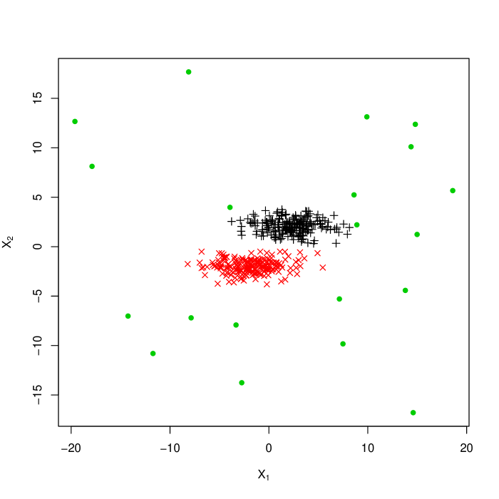
Figure 1: Scatterplot of the artificial data of Section 5.2. Noise is represented by green bullets.

5.2.1 Model-based clustering

We start with a model-based clustering analysis by considering all the fourteen models in Table 1 and a number $G$ of clusters ranging from 1 to 4, resulting in 56 different models. The following command R> res1 <- CNmixt(X, model = NULL, G = 1:4, parallel = TRUE) With G = 1, some models are equivalent, so only one model from each set of equivalent models will be run.

Using 8 cores

Best model according to AIC has G = 3 group(s) and parsimonious structure VVI

Best model according to AICc, AICu, AIC3, AWE, BIC, CAIC, ICL has G = 2 group(s) and parsimonious structure EEI performs the ECM-fitting of the models and returns an object of class ContaminatedMixt. Because several models have to be fitted, parallel computation is convenient; it is set with the argument parallel = TRUE. The number of CPU cores used is printed at video and it is followed, after a few seconds, by a description of the best model according to each of the 8 criteria in Table 2. Here, we can note as all the criteria, apart from the AIC, agree in suggesting a model with $G=2$ clusters and the true but unknown parsimonious structure EEI. To find out more about the model selected by the BIC, we run the command R> summary(res1) ———————————- Best fitted model according to BIC ———————————- log.likelihood n par BIC -1835.8 420 11 -3738

Clustering table: 1 2 209 211

Prior: group 1 = 0.4965, group 2 = 0.5035 Model: EEI (diagonal, equal volume and shape) with 2 components

Variables Means: group 1 group 2 X.1 -1.8564 2.3207 X.2 -1.9783 2.0697

Variance-covariance matrices: Component 1 X.1 X.2 X.1 5.0324 0.00000 X.2 0.0000 0.51525 Component 2 X.1 X.2 X.1 5.0324 0.00000 X.2 0.0000 0.51525

Alpha 0.9506963 0.9485337

Eta 86.44625 99.15542 As we can note from the estimates $\widehat{\eta}_{1}=86.44625$ and $\widehat{\eta}_{2}=99.15542$, there is a large enough degree of contamination in the two clusters, which together contributes to capture the underlying noise (see also the estimates $\widehat{\alpha}_{1}=0.9506963$ and $\widehat{\alpha}_{2}=0.9485337$). In order to evaluate the agreement of the obtained clustering with respect to the true one, we can adopt the agree() function, included in the package, in the following way R> agree(res1, givgroup = group) groups givgroup 1 2 bad points 1 0 200 0 2 200 0 0 3 0 2 18 Apart from two bad points which are erroneously attributed to group 1, the obtained classification is in agreement with the true one. Note that these misclassifications are not necessarily an error: the way the noisy points are inserted into the data makes possible that some of them may lay in the same range of good points and, as such, these points are detected as good points by the model. A plot of the clustering results for the best BIC model is displayed with the command (Figure 2) R> plot(res1, contours = TRUE, asp = 1, xlab = expression(X[1]), + ylab = expression(X[2]))

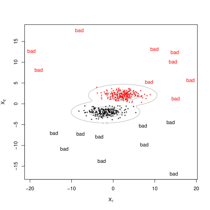
Figure 2: Clustering results from the model selected by the BIC on the artificial data of Section 5.2. Isodensities of the model are superimposed on the plot.

Isodensities are also displayed (contours = TRUE). Results in Figure 2 look similar to those in Figure 1.

5.2.2 Model-based classification

On the same data, we can also suppose to know the cluster membership of some of the available observations and evaluate the classification of the remaining ones. Via the commands R> indlab <- sample(1:400, 20) R> lab <- group[indlab] R> res2 <- CNmixt(X, G = 2, model = "EEI", ind.label = indlab, label = lab) Estimating model EEI with G = 2:********************************************* **********************************************

Estimated one model with G = 2 group(s) and parsimonious structure EEI we firstly randomly select twenty good observations to be considered as labeled, and then we fit the EEI model (model = "EEI"), with $G=2$ clusters, assuming the groups membership of these observations as known in advance. The position of the labeled observations is contained in the object indlab, while their group membership is given in the object lab. The agreement between the obtained classification and the true classification of the unlabelled observations only can be evaluated via the command R> agree(res2, givgroup = group) groups 1 2 bad points 1 0 193 1 2 186 0 0 3 0 0 20 Naturally, the comparison is automatically focused on the unlabelled observations. As we can see, the results slightly change with respect to the clustering analysis and only one good observation from the first cluster is erroneously detected as bad.

5.3 The wine dataset

This second tutorial uses the wine data set included in the ContaminatedMixt package and available at the UCI machine learning repository http://archive.ics.uci.edu/ml/datasets/Wine. These data are the results of a chemical analysis of wines grown in the same region in Italy but derived from three different cultivars (Barbera, Barolo, and Grignolino). The analysis determined the quantities of $p=13$ constituents (continuous variables) found in each of the three types of wine. Data are loaded with R> data("wine") This command loads a data frame with the first column being a factor indicating the type of wine and the others containing the measurements about the 13 constituents. The plot of these data, displayed in Figure 3, is obtained by R> group <- wine[, 1] R> pairs(wine[, -1], cex = 0.6, pch = c(2, 3, 1)[group], + col = c(3, 4, 2)[group], gap = 0, cex.labels = 0.6)

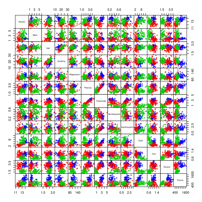
Figure 3: Wine data: Scatterplot matrix with clustering induced by the three cultivars.

The command R> res3 <- CNmixt(wine[, -1], G = 1:4, initialization = "random.soft", + seed = 5, parallel = TRUE) With G = 1, some models are equivalent, so only one model from each set of equivalent models will be run.

Using 8 cores

Best model according to AIC has G = 3 group(s) and parsimonious structure EVV

Best model according to AICc has G = 4 group(s) and parsimonious structure EVE

Best model according to AICu, CAIC has G = 3 group(s) and parsimonious structure EVI

Best model according to AIC3 has G = 2 group(s) and parsimonious structure EVV

Best model according to AWE has G = 3 group(s) and parsimonious structure EEI

Best model according to BIC, ICL has G = 3 group(s) and parsimonious structure EEE fits all the fourteen models for $G\in\left\{1,2,3,4\right\}$, for a total of 56 models. In this case, a random soft initialization is used (initialization = "random.soft") with a pre-specified seed of random generation (seed = 5). The best model, for the most commonly used criteria BIC and ICL, is EEE. The classification performance of this model can be seen via the command R> agree(res3, givgroup = group) groups givgroup 1 2 3 bad points Barbera 44 0 0 4 Barolo 0 0 59 0 Grignolino 0 49 0 22 As we can note, there are not misclassified wines; however, 26 wines are recognized as bad, 22 of which arise from the Grignolino cultivar. Normal and $t$ mixtures do not allow this detection; moreover their classification, as estimated via the packages mixture and teigen, is not as good as that provided above (cf. Punzo and McNicholas, 2016). The graphical representation of the classification from the selected model can be obtained via the command (see Figure 4) R> pairs(res3, cex = 0.6, gap = 0, cex.labels = 0.6)

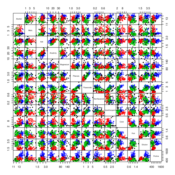
Figure 4: Wine data: Classification results from the model selected by BIC and ICL. Bad points are represented by black bullets.

6 Conclusions

In this paper, we have introduced ContaminatedMixt, a package for the R software environment, specifically conceived for fitting and disseminating parsimonious mixtures of multivariate contaminated normal distributions. Although these models have been originally proposed for clustering applications (Punzo and McNicholas, 2016), their use has been here extended to model-based classification, where information about the group membership of some of the observations is available. The package is also meant to be a user-friendly tool for an automatic detection of mild outliers (also referred to as bad points herein). Advantageously, computation can take advantage of parallelization on multicore PCs and computer clusters, when a comparison among different models is needed. This is handy when, as it is often the case in practical applications, the number of clusters and/or the covariance structure of the model is not a priori known. We believe our package may be a practical tool supporting academics and practitioners who are involved in robust cluster/classification analysis applications.

References

- Aitken (1926) Aitken AC (1926). “On Bernoulli’s Numerical Solution of Algebraic Equations.” In Proceedings of the Royal Society of Edinburgh, volume 46, pp. 289–305.
- Aitkin and Wilson (1980) Aitkin M, Wilson GT (1980). “Mixture Models, Outliers, and the EM Algorithm.” Technometrics, 22(3), 325–331.
- Akaike (1973) Akaike H (1973). “Information Theory and an Extension of Maximum Likelihood Principle.” In BN Petrov, F Csaki (eds.), Second International Symposium on Information Theory, pp. 267–281. Akademiai Kiado, Budapest.
- Andrews and McNicholas (2012) Andrews JL, McNicholas PD (2012). “Model-Based Clustering, Classification, and Discriminant Analysis via Mixtures of Multivariate -Distributions.” Statistics and Computing, 22(5), 1021–1029.
- Andrews et al. (2011) Andrews JL, McNicholas PD, Subedi S (2011). “Model-Based Classification via Mixtures of Multivariate -Distributions.” Computational Statistics and Data Analysis, 55(1), 520–529.
- Andrews et al. (2015) Andrews JL, Wickins JR, Boers NM, McNicholas PD (2015). \pkgteigen: Model-Based Clustering and Classification with the Multivariate Distribution. Version 2.1.0 (2015-11-20), URL http://CRAN.R-project.org/package=teigen.
- Bagnato and Punzo (2013) Bagnato L, Punzo A (2013). “Finite Mixtures of Unimodal Beta and Gamma Densities and the -Bumps Algorithm.” Computational Statistics, 28(4), 1571–1597.
- Banfield and Raftery (1993) Banfield JD, Raftery AE (1993). “Model-Based Gaussian and Non-Gaussian Clustering.” Biometrics, 49(3), 803–821.
- Barnett and Lewis (1994) Barnett V, Lewis T (1994). Outliers in Statistical Data. Wiley Series in Probability & Statistics. Wiley. URL https://books.google.it/books?id=B44QAQAAIAAJ.
- Becker and Gather (1999) Becker C, Gather U (1999). “The Masking Breakdown Point of Multivariate Outlier Identification Rules.” Journal of the American Statistical Association, 94(447), 947–955.
- Berkane and Bentler (1988) Berkane M, Bentler PM (1988). “Estimation of Contamination Parameters and Identification of Outliers in Multivariate Data.” Sociological Methods & Research, 17(1), 55–64.
- Biecek et al. (2012) Biecek P, Szczurek E, Vingron M, Tiuryn J (2012). “The \proglangR Package \pkgbgmm: Mixture Modeling with Uncertain Knowledge.” Journal of Statistical Software, 47(3), 1–31. ISSN 1548-7660. URL http://www.jstatsoft.org/v47/i03.
- Biernacki et al. (2000) Biernacki C, Celeux G, Govaert G (2000). “Assessing a Mixture Model for Clustering with the Integrated Completed Likelihood.” Pattern Analysis and Machine Intelligence, IEEE Transactions on, 22(7), 719–725.
- Biernacki et al. (2003) Biernacki C, Celeux G, Govaert G (2003). “Choosing Starting Values for the EM Algorithm for Getting the Highest Likelihood in Multivariate Gaussian Mixture Models.” Computational Statistics & Data Analysis, 41(3–4), 561–575.
- Bock (2002) Bock HH (2002). “Clustering Methods: From Classical Models to New Approaches.” Statistics in Transition, 5(5), 725–758.
- Böhning (2000) Böhning D (2000). Computer-Assisted Analysis of Mixtures and Applications: Meta-analysis, Disease Mapping and Others, volume 81 of Monographs on Statistics and Applied Probability. Chapman & Hall/CRC, London.
- Bozdogan (1987) Bozdogan H (1987). “Model Selection and Akaikes’s Information Criterion (AIC): The General Theory and Its Analytical Extensions.” Psycometrika, 52, 345–370.
- Bozdogan (1994) Bozdogan H (1994). “Theory & Methodology of Time Series Analysis.” In Proceedings of the First US/Japan Conference on the Frontiers of Statistical Modeling: An Informational Approach, volume 1. Kluwer Academic Publishers, Dordrecht.
- Browne et al. (2015) Browne RP, ElSherbiny A, McNicholas PD (2015). \pkgmixture: Mixture Models for Clustering and Classification. Version 1.4 (2015-03-10), URL http://CRAN.R-project.org/package=mixture.
- Browne and McNicholas (2012) Browne RP, McNicholas PD (2012). “Model-based clustering, classification, and discriminant analysis of data with mixed type.” Journal of Statistical Planning and Inference, 142(11), 2976–2984.
- Celeux and Govaert (1995) Celeux G, Govaert G (1995). “Gaussian Parsimonious Clustering Models.” Pattern Recognition, 28(5), 781–793.
- Dang et al. (2015) Dang UJ, Browne RP, McNicholas PD (2015). “Mixtures of Multivariate Power Exponential Distributions.” Biometrics.
- Davies and Gather (1993) Davies L, Gather U (1993). “The Identification of Multiple Outliers.” Journal of the American Statistical Association, 88(423), 782–792.
- Dean et al. (2006) Dean N, Murphy TB, Downey G (2006). “Using Unlabelled Data to Update Classification Rules with Applications in Food Authenticity Studies.” Journal of the Royal Statistical Society: Series C (Applied Statistics), 55(1), 1–14.
- Dempster et al. (1977) Dempster AP, Laird NM, Rubin DB (1977). “Maximum Likelihood from Incomplete Data via the EM Algorithm.” Journal of the Royal Statistical Society. Series B (Methodological), 39(1), 1–38.
- Fraley and Raftery (1998) Fraley C, Raftery AE (1998). “How Many Clusters? Which Clustering Method? Answers Via Model-Based Cluster Analysis.” Computer Journal, 41(8), 578–588.
- Fraley and Raftery (2007) Fraley C, Raftery AE (2007). “Model-based Methods of Classification: Using the \pkgmclust Software in Chemometrics.” Journal of Statistical Software, 18(6), 1–13. URL http://www.jstatsoft.org/v18/i06.
- Fraley et al. (2015) Fraley C, Raftery AE, Scrucca L, Murphy TB, Fop M (2015). \pkgmclust: Normal Mixture Modelling for Model-Based Clustering, Classification, and Density Estimation. Version 5.1 (2015-10-27), URL http://cran.r-project.org/web/packages=mclust.
- Fritz et al. (2012) Fritz H, García-Escudero LA, Mayo-Iscar A (2012). “\pkgtclust: An \proglangR Package for a Trimming Approach to Cluster Analysis.” Journal of Statistical Software, 47(12), 1–26.
- Gallegos and Ritter (2009) Gallegos MT, Ritter G (2009). “Trimmed ML Estimation of Contaminated Mixtures.” Sankhyā: The Indian Journal of Statistics, Series A, 71(2), 164–220.
- Gómez-Villegas et al. (2011) Gómez-Villegas MA, Gómez-Sánchez-Manzano E, Maín P, Navarro H (2011). “The Effect of Non-Normality in the Power Exponential Distributions.” In L Pardo, N Balakrishnan, MA Gil (eds.), Modern Mathematical Tools and Techniques in Capturing Complexity, Understanding Complex Systems, pp. 119–129. Springer, Berlin Heidelberg.
- Hathaway (1986) Hathaway RJ (1986). “A Constrained EM Algorithm for Univariate Normal Mixtures.” Journal of Statistical Computation and Simulation, 23(3), 211–230.
- Hennig (2002) Hennig C (2002). “Fixed Point Clusters for Linear Regression: Computation and Comparison.” Journal of Classification, 19(2), 249–276.
- Hurvich and Tsai (1989) Hurvich CM, Tsai CL (1989). “Regression and Time Series Model Selection in Small Samples.” Biometrika, 76(2), 297–307.
- Ingrassia (2004) Ingrassia S (2004). “A Likelihood-Based Constrained Algorithm for Multivariate Normal Mixture Models.” Statistical Methods and Applications, 13(2), 151–166.
- Karlis and Xekalaki (2003) Karlis D, Xekalaki E (2003). “Choosing Initial Values for the EM Algorithm for Finite Mixtures.” Computational Statistics & Data Analysis, 41(3–4), 577–590.
- Lange et al. (1989) Lange KL, Little RJA, Taylor JMG (1989). “Robust Statistical Modeling using the Distribution.” Journal of the American Statistical Association, 84(408), 881–896.
- Lebret et al. (2015) Lebret R, Iovleff S, Langrognet F, Biernacki C, Celeux G, Govaert G (2015). \pkgRmixmod: An interface of \proglangMIXMOD. Version 2.0.3 (2015-10-06), URL http://cran.r-project.org/web/package=Rmixmod.
- Leisch and Grün (2015) Leisch F, Grün B (2015). CRAN Task View: Cluster Analysis & Finite Mixture Models. Version 2015-07-24, URL https://cran.r-project.org/web/views/Cluster.html.
- Lindsay (1995) Lindsay BG (1995). Mixture Models: Theory, Geometry and Applications, volume 5. NSF-CBMS Regional Conference Series in Probability and Statistics, Institute of Mathematical Statistics, Hayward, California.
- Little (1988) Little RJA (1988). “Robust Estimation of the Mean and Covariance Matrix from Data with Missing Values.” Applied Statistics, 37(1), 23–38.
- Maruotti and Punzo (2016) Maruotti A, Punzo A (2016). “Model-Based Time-Varying Clustering of Multivariate Longitudinal Data with Covariates and Outliers.” Computational Statistics & Data Analysis. 10.1016/j.csda.2016.05.024.
- McLachlan and Basford (1988) McLachlan GJ, Basford KE (1988). Mixture Models: Inference and Applications to Clustering. Marcel Dekker, New York.
- McLachlan and Krishnan (2007) McLachlan GJ, Krishnan T (2007). The EM Algorithm and Extensions. John Wiley & Sons, New York.
- McLachlan and Peel (1998) McLachlan GJ, Peel D (1998). “Robust Cluster Analysis via Mixtures of Multivariate -Distributions.” In A Amin, D Dori, P Pudil, H Freeman (eds.), Advances in Pattern Recognition, volume 1451 of Lecture Notes in Computer Science, pp. 658–666. Springer, Berlin - Heidelberg.
- McNicholas (2010) McNicholas PD (2010). “Model-Based Classification using Latent Gaussian Mixture Models.” Journal of Statistical Planning and Inference, 140(5), 1175–1181.
- McNicholas et al. (2015) McNicholas PD, ElSherbiny A, Jampani R, McDaid A, Murphy B, Banks L (2015). \pkgpgmm: Parsimonious Gaussian Mixture Models. Version 1.2 (2015-04-28), URL http://cran.r-project.org/web/package=pgmm.
- McQuarrie et al. (1997) McQuarrie A, Shumway R, Tsai CL (1997). “The Model Selection Criterion AICu.” Statistics & Probability Letters, 34(3), 285–292.
- Meng and Rubin (1993) Meng XL, Rubin DB (1993). “Maximum Likelihood Estimation via the ECM Algorithm: A General Framework.” Biometrika, 80(2), 267–278.
- Peel and McLachlan (2000) Peel D, McLachlan GJ (2000). “Robust Mixture Modelling using the Distribution.” Statistics and Computing, 10(4), 339–348.
- Punzo (2014) Punzo A (2014). “Flexible Mixture Modeling with the Polynomial Gaussian Cluster-Weighted Model.” Statistical Modelling, 14(3), 257–291.
- Punzo et al. (2016) Punzo A, Browne RP, McNicholas PD (2016). “Hypothesis Testing for Mixture Model Selection.” Journal of Statistical Computation and Simulation. 10.1080/00949655.2015.1131282.
- Punzo and Maruotti (2016) Punzo A, Maruotti A (2016). “Clustering Multivariate Longitudinal Observations: The Contaminated Gaussian Hidden Markov Model.” Journal of Computational and Graphical Statistics, pp. 1–32. 10.1080/10618600.2015.1089776.
- Punzo and McNicholas (2014a) Punzo A, McNicholas PD (2014a). “Robust Clustering in Regression Analysis via the Contaminated Gaussian Cluster-Weighted Model.” arXiv.org e-print 1409.6019, available at: http://arxiv.org/abs/1409.6019.
- Punzo and McNicholas (2014b) Punzo A, McNicholas PD (2014b). “Robust High-Dimensional Modeling with the Contaminated Gaussian Distribution.” arXiv.org e-print 1408.2128, available at: http://arxiv.org/abs/1408.2128.
- Punzo and McNicholas (2016) Punzo A, McNicholas PD (2016). “Parsimonious Mixtures of Multivariate Contaminated Normal Distributions.” Biometrical Journal.
- \proglangR Core Team (2015) \proglangR Core Team (2015). \proglangR: A Language and Environment for Statistical Computing. \proglangR Foundation for Statistical Computing, Vienna, Austria. URL https://www.R-project.org/.
- Ritter (2015) Ritter G (2015). Robust Cluster Analysis and Variable Selection, volume 137 of Chapman & Hall/CRC Monographs on Statistics & Applied Probability. CRC Press.
- Schwarz (1978) Schwarz G (1978). “Estimating the Dimension of a Model.” The Annals of Statistics, 6(2), 461–464.
- Subedi et al. (2013) Subedi S, Punzo A, Ingrassia S, McNicholas PD (2013). “Clustering and Classification via Cluster-Weighted Factor Analyzers.” Advances in Data Analysis and Classification, 7(1), 5–40.
- Subedi et al. (2015) Subedi S, Punzo A, Ingrassia S, McNicholas PD (2015). “Cluster-Weighted -Factor Analyzers for Robust Model-Based Clustering and Dimension Reduction.” Statistical Methods and Applications, 24(4), 623–649.
- Tukey (1960) Tukey JW (1960). “A Survey of Sampling from Contaminated Distributions.” In I Olkin (ed.), Contributions to Probability and Statistics: Essays in Honor of Harold Hotelling, Stanford Studies in Mathematics and Statistics, chapter 39, pp. 448–485. Stanford University Press, California.
- Zhang and Liang (2010) Zhang J, Liang F (2010). “Robust Clustering using Exponential Power Mixtures.” Biometrics, 66(4), 1078–1086.