Percolation on trees as a Brownian excursion:
from Gaussian to Kolmogorov-Smirnov to Exponential statistics

Abstract

We calculate the distribution of the size of the percolating cluster on a tree in the subcritical, critical and supercritical phase. We do this by exploiting a mapping between continuum trees and Brownian excursions, and arrive at a diffusion equation with suitable boundary conditions. The exact solution to this equation can be conveniently represented as a characteristic function, from which the following distributions are clearly visible: Gaussian (subcritical), Kolmogorov-Smirnov (critical) and exponential (supercritical). In this way we provide an intuitive explanation for the result reported in R. Botet and M. Płoszajczak, Phys. Rev. Lett 95, 185702 (2005) for critical percolation.

I Introduction

Mappings that connect seemingly unrelated models are regularly used in statistical physics. They not only facilitate calculations but provide additional intuition about the original models. Well-known examples include the Ising model interpretation for a lattice gasCardy (1996), the bosonic interpretation for the partitioning of an integer into summandsAuluck and Kothari (1946), or the Coulomb gas interpretation for the eigenvalues of certain random matricesMehta (2004). In practice, the coincidence in distribution of an observable in one model may spur the search for a mapping to its counterpart observable in another model. In this Letter, we adopt this route inspired by the Kolmogorov-Smirnov (KS) distribution, which has been noticed in a variety of contexts. It is the distribution of a test statistic for comparing between empirical and theoretical distribution functions, and is well understood to describe the absolute maximum value of a Brownian bridgeDoob (1946). With this insight, it can be related to other Brownian observablesBiane et al. (2001). More surprisingly, it is the distribution of the integrated mean-squared fluctuations of a periodic Brownian signalWatson (1961), and therefore also accounts for the roughness of a 1d periodic Edwards-Wilkinson interface in the steady stateFoltin et al. (1994). It also describes the sizes of clusters in a mean-field aggregation processBotet and Płoszajczak (2005).

This paper focuses on the finite-size scaled distribution of percolating cluster sizes on a Bethe lattice at the critical point, first computed by Botet and PłoszajczakBotet and Płoszajczak (2005); Botet (2011) to be the KS distribution. We demonstrate that there is indeed a connection to Brownian motions, thereby obtaining a more intuitive understanding of their result. In this way, we demystify the coincidence in distribution and bring the result into the existing fold of knowledge about Brownian motions and associated observablesBiane et al. (2001); Majumdar (2005).

II Setting up the problem

We consider site percolation on a finite Bethe lattice of size $L$, coordination number $z$ and site occupation probability $p$, with critical occupation probability $p_{c}=1/(z-1)$Stauffer and Aharony (1994). There is a distinguishable site at the center, called the root, from which distances or ‘heights’ to other sites can be measured. With a subsequent mapping to Brownian excursions in mind, it is convenient to define the root to be at $h=1$. Neighboring sites in the first generation are then at $h=2$, sites at the boundary at $h=L$, etc. We say that the system percolates if there is at least one path of occupied sites from the root to any boundary site. The percolating cluster, containing the root, can be thought of as a rooted tree of fixed height.

The size $S$ of the percolating cluster is the number of sites forming the cluster that contains the root (which may include more than one path to the boundary). If the system does not percolate, we set $S=0$ for convenience.

In what follows, we will be concerned with the distribution of the size of the percolating cluster given that the system percolates,

$$\mathcal{P}(s)\equiv\mathrm{Prob}[S=s:S>0].$$ (1)

In particular, we will direct our attention to the limit of large system sizes $L\gg 1$. A well-normalized limiting distribution for the rescaled percolating cluster size will therefore depend on how $S$ scales with $L$ for different values of $p$.

III Mapping to Brownian Excursion

The well-known depth-first searchAldous (1993) (also known as a Harris walk) gives a bijection between rooted trees and excursions. Here we make use of an asymptotic version of this technique for $L\gg 1$ to map the percolation problem to a Brownian excursion with specific boundary conditions.

Consider a realization of the percolating cluster, traversed in depth-first search order starting from the root at time $i=0$, see Fig. 1. Each edge is traversed exactly twice, once in each direction, and the pairs $(i,h(i))$ form a positive walk of length $2S$. To have a well-defined excursion that terminates at $h=0$ once the tree has been traversed and not before, an up-step and a down-step is appended to the beginning and end of the path.

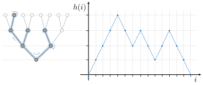
Figure 1: The correspondence between trees and positive paths in a system of size $L=4$. The percolating cluster has size $S=7$, and the associated walk has duration $T=2S=14$. Left: The percolating cluster, traversed in depth-first search order, as indicated by the arrows next to the edges. Right: The associated path, with an initial and final step appended so that the walk does not return to $h=0$ before the entire tree has been traversed.

For large $L$, the walk $(i,h(i))$ can be approximated by a Brownian excursion. If we further think of percolation on the Bethe lattice as a Galton-Watson branching process with binomial offspring distribution $X\sim\mathcal{B}(z-1,p)$, then the drift $v$, diffusion constant $D$ and initial condition $x_{0}$ of the associated excursion can be determined simply by inspecting and matching some well-known results. For example, the probability for an unbiased excursion to reach level $k$ before 0, starting from $x_{0}$, is $x_{0}/k$ (the gambler’s ruin probability); while the probability for a critical branching process to survive at least $k$ generations is $2/(\mathrm{Var}[X]k)$Harris (1963); Athreya and Ney (2004). This result, together with the matching of the first two cumulants of the total population of a subcritical branching processSuhov and Kelbert (2014) with those of the corresponding Brownian excursion, leads to the identifications:

$$v=\frac{\mathrm{E}[X]-1}{\mathrm{Var}[X]},\quad D=\frac{1}{\mathrm{Var}[X]},\quad x_{0}=\frac{2}{\mathrm{Var}[X]},$$ (2)

where $\mathrm{E}[X]=(z-1)p$ and $\mathrm{Var}[X]=(z-1)p(1-p)$. This is in agreement with the known rescaling of the so-called contour process Bennies and Kersting (2000). In addition, the system is conditioned to percolate, so that the associated walk must reach height $h(j)=L$ for some $0<j<2S$ before returning to the origin for the first time at $i=2S$. In summary, the large $L$ limit of the walk $(i,h(i))$ corresponds to a Brownian excursion of maximum height $L$, drift $v$ and diffusion constant $D$. The (random) duration $T$ of this Brownian excursion equals $2S$ by construction.

Proper convergence of a positive walk to a Brownian excursion is formally only reached after rescaling lengths appropriately, but we will only take this step at the very end of our calculations, once the scaling of $S$ with $L$, as a function of $p$, has been calculated. Formal proofs of convergence in similar setups can be found in the related literature on continuum random trees. For instance, AldousAldous (1993) shows that if certain families of trees are constrained to have a fixed large number of nodes, then its associated Harris walks converge to the standard Brownian excursion of length 1; while Le GallGall (2005) also considers constraints related to the maximum height. In both cases it is shown that, under certain mild conditions, all families of trees (i.e., all lattices) lead to the same universal results.

We have thus set up a mapping between percolation in a finite Bethe lattice and a Brownian excursion with a reflecting boundary, and explicitly related their parameters, Eq. (2). In what follows, we will compute the distribution of $T$ in the Brownian excursion setting, and show that the results agree, as expected, with simulations of percolation in a Bethe lattice.

IV Brownian Excursion

The Brownian excursion of fixed height $L$ corresponding to our problem can be decomposed into two paths (see Fig. 2): (i) a first path from the origin $x(0)=0$ at time $t=0$ to the boundary $x(T_{1})=L$, taking time $T_{1}$, and (ii) a return path from the reflecting boundary $x(T_{1})=L$ to the origin $x(T)=0$, taking time $T_{2}=T-T_{1}$. Note that the first path involves a conditional exit at $x=L$ such that that boundary is effectively absorbing for $t<T_{1}$. Readers experienced with Brownian processes will recognize $T_{1}$ as the hitting time to reach $L$ of a 3d Bessel processBiane et al. (2001).

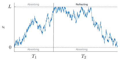
Figure 2: A Brownian excursion, conditioned to reach $x(t)=L$ for some $0<t<T=T_{1}+T_{2}$, decomposed into (i) the path from $x=0$ that reaches $x=L$ for the first time, (ii) the return path from $x=L$ back to $x=0$.

IV.1 Diffusion equation with drift

The distributions of $T_{1}$ and $T_{2}$ are most conveniently calculated by working with the Laplace transform of the diffusion equation with drift:

$$\left[-D\partial_{xx}+v\partial_{x}+\lambda\right]\hat{\phi}(x,\lambda)=\delta(x-x_{0})$$ (3)

where $\phi(x,\lambda)$ is the Laplace transform with respect to time of the density function with initial condition $x(0)=x_{0}$. According to the usual recipeRedner (2001), this equation is solved with combinations of exponentials respecting the boundary conditions, and fluxes are computed at the relevant boundaries. These calculations furnish the Laplace transformed first passage densities $j_{1}(\lambda)$ and $j_{2}(\lambda)$ associated with $T_{1}$ and $T_{2}$.

IV.2 First path: A + A

To calculate $T_{1}$ for the first path of the decomposition, absorbing boundaries are required at both at $x=0$ and $x=L$,

$$\hat{\phi}_{AA}(0,\lambda) =0$$ (4)

$$\hat{\phi}_{AA}(L,\lambda) =0,$$ (5)

together with a conditional exit $x=L$. $\hat{\phi}_{AA}$ satisfying the absorbing boundaries takes the form

$$\hat{\phi}_{AA}(x,\lambda)=\frac{2e^{v(x-x_{0})/2D}}{\rho\sinh(\rho L/2D)}\sinh(\rho x_{0}/2D)\sinh(\rho(L-x)/2D)$$ (6)

where $\rho:=\sqrt{v^{2}+4\lambda D}$. The conditional exit probability at $x=L$ isRedner (2001)

$$\mathrm{Prob}(\text{exit at }x=L)=\frac{1-e^{-vx_{0}/D}}{1-e^{-Lv/D}}$$ (7)

so that the flux at the boundary $x=L$ is

$$j_{1}(\lambda) =\lim_{x_{0}\to 0}\frac{-D\hat{\phi}^{\prime}_{AA}(L,\lambda)}{\mathrm{Prob}(\text{exit at }x=L)}$$ (8)

$$=\frac{\rho}{v}\frac{\sinh(Lv/2D)}{\sinh(\rho L/2D)}$$ (9)

IV.3 Return path: A + R

To calculate $T_{2}$ for the second path of the decomposition, an absorbing boundary is required at $x=0$

$$\hat{\phi}_{AR}(0,\lambda)=0$$ (10)

and a Dirac $\delta$-pulse is injected at $x=L$ as an initial condition, which in Laplace space is equivalent to the boundary condition

$$-v\hat{\phi}_{AR}(L,\lambda)+D\hat{\phi}^{\prime}_{AR}(L,\lambda)=1$$ (11)

$\hat{\phi}_{AR}$ satisfying these boundary conditions is

$$\hat{\phi}_{AR}(x,\lambda)=\frac{2e^{v(x-L)/2D}\,\sinh(\rho x/2D)}{\rho\cosh(\rho L/2D)-v\sinh(\rho L/2D)},$$ (12)

so that the flux at the boundary $x=0$ is

$$j_{2}(\lambda) =D\hat{\phi}^{\prime}_{AR}(0,\lambda)$$ (13)

$$=\frac{\rho\,e^{-Lv/2D}}{\rho\cosh(\rho L/2D)-v\sinh(\rho L/2D)}.$$ (14)

IV.4 Entire excursion

The total time to go from the origin to the boundary at $x=L$, and then from the boundary back to the origin is $T=T_{1}+T_{2}$. Since $T_{1}$ and $T_{2}$ are independent, the Laplace transform of the density of the total time $T$ is the product

$$j(\lambda) =j_{1}(\lambda)\cdot j_{2}(\lambda)$$

$$=\frac{\rho^{2}}{v}\frac{\sinh(Lv/2D)}{\sinh(\rho L/2D)}\times$$

$$\frac{e^{-Lv/2D}}{\rho\cosh(\rho L/2D)-v\sinh(\rho L/2D)}$$ (15)

IV.5 Critical case

Critical percolation with $p=p_{c}=1/(z-1)$ maps to Brownian motion with zero drift. Taking the limit $v\to 0$ in Eq.(15),

$$j_{1}^{(c)}(\lambda) =\frac{L\sqrt{\lambda/D}}{\sinh(L\sqrt{\lambda/D})}$$ (16)

$$j_{2}^{(c)}(\lambda) =\frac{1}{\cosh(L\sqrt{\lambda/D})}$$ (17)

$$j^{(c)}(\lambda) =\frac{2L\sqrt{\lambda/D}}{\sinh(2L\sqrt{\lambda/D})}.$$ (18)

Interestingly, $j_{1}^{(c)}$ and $j^{(c)}$ are Laplace transforms of the same KS distribution on different scales. $j_{2}^{(c)}$ is also the Laplace transform of many observables of Brownian motions, seeBiane et al. (2001) for a review.

IV.6 General case

For general choices of $v$ (or, equivalently, $p$), the full solution in Eq. (15) cannot be inverted explicitly, and one must resort to numerical inversion. Fig 3 shows a family of percolating cluster size distributions, all rescaled by their means.

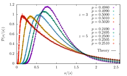
Figure 3: The rescaled distribution of the percolating cluster size, for different values of $z$ and $p$ and fixed system size $L=10^{3}$. Simulations (colored symbols) agree with theory (black line), which is obtained via numerical inversion of Eq.(15). 

The distributions are independent of coordination number $z$ as expected, but clearly depend on $p$. For $p\neq p_{c}$ (and fixed $L$), the distributions can be thought of as flowing away from the non-trivial fixed point, represented by the KS distribution (middle, blue curve).

To better understand these flows towards trivial fixed points (in the language of renormalization-group (RG)) for $p\to 0$ and $p\to 1$, it is convenient to standardize the distributions to zero mean and unit standard deviation. Since Eq. (15) is the moment generating function for $T$, these cumulants can be constructed as usual by differentiating once (first moment) or twice (second moment) with respect to $\lambda$, and taking $\lambda\to 0$. For the mean $\mu:=\langle T\rangle$ we find

$$\mu\,\frac{v^{2}}{D}=\mathcal{F}(Lv/D),$$ (19)

where the scaling function

$$\mathcal{F}(x)=e^{x}-3+\frac{2x}{e^{x}-1}$$ (20)

behaves as $e^{x}$ for $x\gg 1$, $x^{2}$ for $x\to 0$, and $x$ for $x\ll-1$. For fixed $v$ and $D$, the scaling behavior of $\mu$ is therefore

$$\mu=\begin{cases}\frac{D}{v^{2}}e^{Lv/D},&\quad L\gg 1,v>0\\ \frac{2}{3D}L^{2},&\quad L\gg 1,v=0\\ \frac{2}{|v|}L,&\quad L\gg 1,v<0.\end{cases}$$ (21)

Expressions can likewise be obtained for the standard deviation $\sigma:=\sqrt{\langle T^{2}\rangle-\langle T\rangle^{2}}$ (not shown).

Given $\mu$ and $\sigma$, we arrive at a standardized characteristic function $\mathcal{G}(k;Lv/D)$ from Eq. (15) by (i) replacing $\lambda\to-ik$, to change from Laplace to Fourier space, (ii) multiplying by $\exp(-ik\mu)$ to translate the distribution to zero mean, and (iii) replacing $k\to k/\sigma$, to scale the distribution to unit standard deviation. Note that the ratio $\mu/\sigma$ is a function of $Lv/D$ alone. Thus, $\mathcal{G}(k;Lv/D)$ describes a family of probability distributions parameterized by $Lv/D$.

As a result of this standardization, all distributions $\mathcal{G}(k;Lv/D)$ have zero mean and unit standard deviation. However, higher cumulants $\kappa_{n}$ will depend on $Lv/D$. These differences can be visualized by plotting the skewness $\kappa_{3}$ versus the kurtosis $\kappa_{4}-3$, as depicted in Fig. 4. Three regimes are particularly noteworthy: (i) $Lv/D\to-\infty$ (subcritical fixed point), (ii) $Lv/D\to 0$ (critical fixed point), (iii) $Lv/D\to\infty$ (supercritical fixed point). With the help of Mathematica, we can obtain full expressions for $(\kappa_{3},\kappa_{4}-3)$ as a function of $Lv/D$. In the three above regimes these reduce to (i) $(2,6)$, (ii) $(4\sqrt{10}/7,36/7)$, (iii) $(0,0)$, corresponding to exponential, KS and Gaussian distributions, respectively. These three fixed points are marked in Fig. 4 as solid circles.

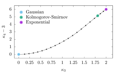
Figure 4: Centered skewness $\kappa_{3}$ and kurtosis $\kappa_{4}-3$ for the standardized solution described by $\mathcal{G}(k;Lv)$. Solid circles from left to right correspond to the fixed points: Gaussian (subcritical), KS (critical), Exponential (supercritical).

A heuristic explanation for the sub and supercritical limits is as follows: the overall behavior of $T$ is dominated by $T_{2}$ ($T_{1}$ is insensitive to the sign of $v$, which can be seen from the fact that (6) is an even function of $v$). When $v<0$, $T_{2}$ is approximately the ballistic travel time from $x=L$ to $x=0$, with a Gaussian correction coming from diffusion. When $v>0$, $T_{2}$ is dominated by the rare event that the motion escapes the drift that keeps returning it to the reflecting boundary at $x=L$. This rare event process is consistent with exponential tails.

We briefly comment on how our method differs from that of Botet and PłoszajczakBotet and Płoszajczak (2005), the full details of which are presented inBotet (2011). In their method, a recursion is set up between successive generations of the Bethe lattice, encoding the statistical weights of configurations conditioned to percolate. The recursion relation is then Laplace transformed and rescaled by mean percolating cluster size, to yield expressions which are then analyzed asymptotically in the limit of large system size for the critical case $p=p_{c}$. In contrast, our method makes use of a passage from continuum trees to Brownian excursions at the starting point of the calculation, such that the parameters of the Bethe lattice are reincorporated into the diffusion constant and drift of the resulting motion. This makes the subsequent analysis arguably more intuitive, and Eq.(15) gives the entire cluster size distribution for all regimes from the solution of a diffusion problem with drift. Our approach should be universal across different types of trees, in the sense that the fixed point distributions (suitably rescaled) do not depend on underlying microscopic details.

V Conclusion

We have calculated the distribution of the size of the percolating cluster on a tree by interpreting the problem as a type of Brownian excursion. In this way, we give an intuitive explanation for the coincidence in distribution (first noted inBotet and Płoszajczak (2005)) with other observables associated with Brownian motionsBiane et al. (2001). The analysis can be extended off criticality by adding a drift term to the associated diffusion equation. The resulting flows in the space of distributions can be captured by tracking the skewness and kurtosis. Our exact calculation makes an investigation of the various regimes possible in full detail. We expect that such mappings can be used to investigate further properties of branching processes.