Distinguishing number and distinguishing index of neighbourhood corona of two graphs

Abstract

The distinguishing number (index) $D(G)$ ($D^{\prime}(G)$) of a graph $G$ is the least integer $d$ such that $G$ has an vertex labeling (edge labeling) with $d$ labels that is preserved only by a trivial automorphism. The neighbourhood corona of two graphs $G_{1}$ and $G_{2}$ is denoted by $G_{1}\star G_{2}$ and is the graph obtained by taking one copy of $G_{1}$ and $|V(G_{1})|$ copies of $G_{2}$, and joining the neighbours of the $i$th vertex of $G_{1}$ to every vertex in the $i$th copy of $G_{2}$. In this paper we describe the automorphisms of the graph $G_{1}\star G_{2}$. Using results on automorphisms, we study the distinguishing number and the distinguishing index of $G_{1}\star G_{2}$. We obtain upper bounds for $D(G_{1}\star G_{2})$ and $D^{\prime}(G_{1}\star G_{2})$.

Keywords: Distinguishing index; Distinguishing number; neighborhood corona.

AMS Subj. Class.: 05C15, 05E18

1 Introduction

Let $G=(V,E)$ be a simple graph with $n$ vertices. Throughout this paper we consider only simple graphs. The set of all automorphisms of $G$, with the operation of composition of permutations, is a permutation group on $V$ and is denoted by $Aut(G)$. A labeling of $G$, $\phi:V\rightarrow\{1,2,\ldots,r\}$, is $r$-distinguishing, if no non-trivial automorphism of $G$ preserves all of the vertex labels. In other words, $\phi$ is $r$-distinguishing if for every non-trivial $\sigma\in Aut(G)$, there exists $x$ in $V$ such that $\phi(x)\neq\phi(x\sigma)$. The distinguishing number of a graph $G$ has defined by Albertson and Collins [1] and is the minimum number $r$ such that $G$ has a labeling that is $r$-distinguishing. Similar to this definition, Kalinkowski and Pilśniak [6] have defined the distinguishing index $D^{\prime}(G)$ of $G$ which is the least integer $d$ such that $G$ has an edge colouring with $d$ colours that is preserved only by a trivial automorphism. These indices has developed and number of papers published on this subject (see, for example [2, 7, 9]).

We use the following notations: The set of vertices adjacent in $G$ to a vertex of a vertex subset $W\subseteq V$ is the open neighborhood $N_{G}(W)$ of $W$. The closed neighborhood $G[W]$ also includes all vertices of $W$ itself. In case of a singleton set $W=\{v\}$ we write $N_{G}(v)$ and $N_{G}[v]$ instead of $N_{G}(\{v\})$ and $N_{G}[\{v\}]$, respectively. We omit the subscript when the graph $G$ is clear from the context. The complement of $N[v]$ in $V(G)$ is denoted by $\overline{N[v]}$. We denote the degree of a vertex $v$ in graph $G$ by $d_{G}(v)$ and the distance between two vertices $u$ and $w$ in graph $G$, by $dist_{G}(u,w)$. The corona of two graphs $G$ and $H$ which denoted by $G\circ H$ is defined in [4] and there have been some results on the corona of two graphs [3]. In [2] we have studied the distinguishing number and the distinguishing index of corona of two graphs. In this paper we consider another variation of corona of two graphs and study its distinguishing number and distinguishing index. Given simple graphs $G_{1}$ and $G_{2}$, the neighbourhood corona of $G_{1}$ and $G_{2}$, denoted by $G_{1}\star G_{2}$ and is the graph obtained by taking one copy of $G_{1}$ and $|V(G_{1})|$ copies of $G_{2}$ and joining the neighbours of the $i$th vertex of $G_{1}$ to every vertex in the $i$th copy of $G_{2}$ ([5]). Figure 1 shows $P_{4}\star P_{3}$, where $P_{n}$ is the path of order $n$. Liu and Zhu in [8] determined the adjacency spectrum of $G_{1}\star G_{2}$ for arbitrary $G_{1}$ and $G_{2}$ and the Laplacian spectrum and signless Laplacian spectrum of $G_{1}\star G_{2}$ for regular $G_{1}$ and arbitrary $G_{2}$, in terms of the corresponding spectrum of $G_{1}$ and $G_{2}$. Also Gopalapillai in [5] has studied the eigenvalues and spectrum of $G_{1}\star G_{2}$, when $G_{2}$ is regular.

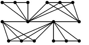
Figure 1: The neighbourhood corona of $P_{4}\star P_{3}$.

In this paper we consider the neighbourhood corona of two graphs and discuss their distinguishing number and index. In the next section, we give a complete description of the automorphisms of neighbourhood corona of two arbitrary graphs. In Section 3, we study the distinguishing number and the distinguishing index of neighbourhood corona of two graphs.

2 Description of automorphisms of $G_{1}\star G_{2}$

In this section we consider the neighbourhood corona of two graphs and describe its automorphisms. Let $G_{i}$ has order $n_{i}$ and size $m_{i}$ $(i=1,2)$. The neighbourhood corona $G_{1}\star G_{2}$ of $G_{1}$ and $G_{2}$ has $n_{1}+n_{1}n_{2}$ vertices and $m_{1}(2n_{2}+1)+n_{1}m_{2}$ edges and when $G_{2}=K_{1}$, the graph $G_{1}\star G_{2}$ is the splitting graph which has defined in [10].

Let $V(G_{1})=\{v_{1},v_{2},\ldots,v_{n_{1}}\}$ and $V(G_{2})=\{u_{1},u_{2},\ldots,u_{n_{2}}\}$. For $i=1,2,\ldots,n_{1}$, let $u^{i}_{1},u^{i}_{2},\ldots,u^{i}_{n_{2}}$ denote the vertices of the $i$th copy of $G_{2}$, with the understanding that $u^{i}_{j}$ is the copy of $u_{j}$ for each $j$. It is clear that the degrees of the vertices of $G_{1}\star G_{2}$ are:

$$d_{G_{1}\star G_{2}}(v_{i})=(n_{2}+1)d_{G_{1}}(v_{i}),~{}~{}i=1,2,\ldots,n_{1}.$$ (1)

$$d_{G_{1}\star G_{2}}(u^{i}_{j})=d_{G_{2}}(u_{j})+d_{G_{1}}(v_{i}),~{}~{}i=1,2,\ldots,n_{1},~{}j=1,2,\ldots,n_{2}.$$ (2)

Now we want to know how an automorphism of $G_{1}\star G_{2}$ acts on the vertices $G_{1}$ and the vertices of copies $G_{2}$. First we state and prove the following lemma.

Lemma 2.1

Let $G_{1}$ and $G_{2}$ be two connected graphs such that $G_{1}\neq K_{1}$ and $f$ be an automorphism of $G_{1}\star G_{2}$ such that $f(v_{i})=u^{k}_{j}$ for some $i,k=1,2,\ldots,n_{1}$ and $j=1,2,\ldots,n_{2}$. Then $d_{G_{1}}(v_{k})>d_{G_{1}}(v_{i})$.

Proof. Since $f(v_{i})=u^{k}_{j}$, so $d_{G_{1}\star G_{2}}(v_{i})=d_{G_{1}\star G_{2}}(u^{k}_{j})$. By Equations (1) and (2) we have $(n_{2}+1)d_{G_{1}}(v_{i})=d_{G_{2}}(u_{j})+d_{G_{1}}(v_{k})$. By contradiction, suppose that $d_{G_{1}}(v_{k})\leqslant d_{G_{1}}(v_{i})$. Hence $(n_{2}+1)d_{G_{1}}(v_{i})\leqslant d_{G_{2}}(u_{j})+d_{G_{1}}(v_{i})$, and so $n_{2}d_{G_{1}}(v_{i})\leqslant d_{G_{2}}(u_{j})$. This contradiction forces us to conclude that $d_{G_{1}}(v_{k})>d_{G_{1}}(v_{i})$. $\square$

By Lemma 2.1 we can prove the following corollary:

Corollary 2.2

Let $G_{1}$ be a connected graph such that $G_{1}\neq K_{1}$ and $f$ be an arbitrary automorphism of $G_{1}\star G_{2}$.

• If $v$ is the vertex of $G_{1}$ with the maximum degree in $G_{1}$, then $f(v)\in G_{1}$.

• If $G_{1}$ is a regular graph, then the restriction of $f$ to $G_{1}$ is an automorphism of $G_{1}$.

We shall obtain some results for the automorphisms of $G_{1}\star G_{2}$.

Lemma 2.3

Let $G_{1}$ and $G_{2}$ be two connected graphs of orders $n_{1}$ and $n_{2}$, respectively, and $n_{1}>1$. Suppose that $f$ is an automorphism of $G_{1}\star G_{2}$ such that the restriction of $f$ to $G_{1}$ is an automorphism of $G_{1}$, and also $f$ maps the copies of $G_{2}$ to each other. Then there are the automorphism $g$ of $G_{1}$ and the automorphisms $h_{1},\ldots,h_{n_{1}}$ of $G_{2}$ such that $f(G_{2}^{i})=(h_{i}(G_{2}))^{k}$, where $v_{k}=g(v_{i})$ and $i,k=1,\ldots,n_{1}$.

Proof. Let $f$ be an automorphism of $G_{1}\star G_{2}$ such that the restriction of $f$ to $G_{1}$ is an automorphism of $G_{1}$, and also $f$ maps the copies of $G_{2}$ to each other. Let $f$ maps the $i$th copy of $G_{2}$, $G_{2}^{i}$, to the $j_{i}$th copy of $G_{2}$, $G_{2}^{j_{i}}$, where $i,j_{i}=1,\ldots,n_{1}$, such that for the fixed numbers $i$ and $j_{i}$ we have $f(u_{k}^{i})=u_{k^{\prime}}^{j_{i}}$, where $k,k^{\prime}=1,\ldots,n_{2}$. Then we define the automorphism $h_{i}$ on $G_{2}$ such that $h_{i}(u_{k})=u_{k^{\prime}}$. To complete the proof we need to show that the map $g$ on $V(G_{1})$ such that $g(v_{i})=v_{j_{i}}$ is an automorphism of $G_{1}$, where $i,j_{i}=1,\ldots,n_{1}$. Without loss of generality we can assume that the vertices $v_{1}$and $v_{2}$ are adjacent, and show that $v_{j_{1}}$ and $v_{j_{2}}$ are adjacent. Since the vertices $v_{1}$ and $v_{2}$ are adjacent, the vertex $v_{1}$ is adjacent to each vertex of $G_{2}^{2}$ (we show this concept by $v_{1}\sim G_{2}^{2}$). Hence $f(v_{1})\sim(h_{2}(G_{2}))^{j_{2}}$, and so $f(v_{1})\sim v_{j_{2}}$ and $v_{1}\sim f^{-1}(v_{j_{2}})$, and thus $f^{-1}(v_{j_{2}})\sim G_{2}^{1}$, and finally we have $v_{j_{2}}\sim G_{2}^{j_{1}}$. With a similar argument we can conclude that $f(v_{2})\sim v_{j_{1}}$, and so $v_{2}\sim f^{-1}(v_{j_{1}})$, and hence $f^{-1}(v_{j_{1}})\sim G_{2}^{2}$, and thus $v_{j_{1}}\sim G_{2}^{j_{2}}$ (see the Figure 2).

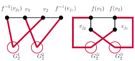
Figure 2: A piece of neighbourhood corona of $G_{1}$ and $G_{2}$ in the proof of Lemma 2.3.

On the other hand, since $f$ maps $G_{2}^{1}$ to $(h_{2}(G_{2}))^{j_{1}}$, we have $d_{G_{1}\star G_{2}}(u_{k}^{1})=d_{G_{1}\star G_{2}}((h_{2}(u_{k}))^{j_{1}})$. We deduce from Equations (1), (2) and $d_{G_{2}}(u_{k})=d_{G_{2}}(h_{2}(u_{k}))$, that $d_{G_{1}}(v_{1})=d_{G_{1}}(v_{j_{1}})$. Similarly, $d_{G_{1}}(v_{2})=d_{G_{1}}(v_{j_{2}})$. Since the restriction of $f$ to $G_{1}$ is an automorphism of $G_{1}$, we have $d_{G_{1}}(v_{1})=d_{G_{1}}(f(v_{1}))$ and $d_{G_{1}}(v_{2})=d_{G_{1}}(f(v_{2}))$. Then

$$d_{G_{1}}(v_{1})=d_{G_{1}}(v_{j_{1}})=d_{G_{1}}(f(v_{1})),~{}d_{G_{1}}(v_{2})=d_{G_{1}}(v_{j_{2}})=d_{G_{1}}(f(v_{2})).$$ (3)

In regard to Equation (3) and Figure 2, there exists the vertices $v_{j_{1}1}$ and $v_{j_{2}1}$ adjacent to vertices $v_{j_{1}}$ and $v_{j_{2}}$, respectively. Thus the vertices $v_{j_{1}1}$ and $v_{j_{2}1}$ are adjacent to $G_{2}^{j_{1}}$ and $G_{2}^{j_{2}}$, respectively, and so $f^{-1}(v_{j_{1}1})\sim G_{2}^{1}$ and $f^{-1}(v_{j_{2}1})\sim G_{2}^{2}$. Hence $f^{-1}(v_{j_{1}1})\sim v_{1}$ and $f^{-1}(v_{j_{2}1})\sim v_{2}$. Since $v_{j_{1}}\sim v_{j_{1}1}$ and $v_{j_{2}}\sim v_{j_{2}1}$, so $f^{-1}(v_{j_{1}})\sim f^{-1}(v_{j_{1}1})$ and $f^{-1}(v_{j_{2}})\sim f^{-1}(v_{j_{2}1})$ (see Figure 3).

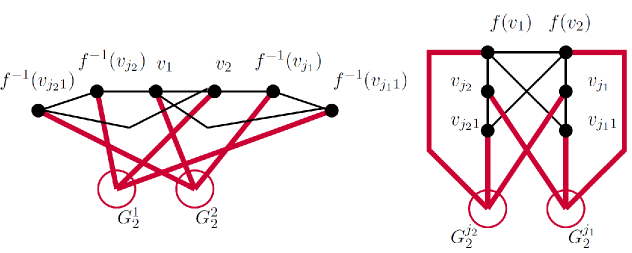
Figure 3: A piece of $G_{1}\star G_{2}$ in the proof of Lemma 2.3.

Note that, for every vertex in $N_{G}(v_{j_{2}})$ such as $x$, we have $x\sim G_{2}^{j_{2}}$. So we see that $f^{-1}(x)\sim G_{2}^{2}$, and so $f^{-1}(x)\sim v_{2}$ (similar argument satisfies for each vertex in $N_{G}(v_{j_{1}})$). In regard to Figure 3 and Equation (3), we need to the other vertex adjacent to $v_{j_{1}}$, such as $x$. If $x$ has been chosen among the nonadjacent vertices to $G_{2}^{j_{2}}$ that has been shown in Figure 3, then with the similar argument as above, we obtain that $f^{-1}(x)$ is adjacent to $v_{1}$, and so Equation (3) dose not satisfy, again. Therefore after finite steps we should choose a vertex adjacent to $v_{j_{1}}$, such as $x$, among the vertices that are adjacent to $G_{2}^{j_{2}}$, otherwise we conclude that the order of $G_{1}$ is infinite and this is a contradiction. By Figure 3 and above information, the vertex $v_{j_{1}}$ is the only vertex that is adjacent to $G_{2}^{j_{2}}$ and is not among the adjacent vertices to $v_{j_{1}}$, in each step. Hence $v_{j_{1}}\sim v_{j_{2}}$, and the result follows. $\square$

Lemma 2.4

Let $G_{1}$ and $G_{2}$ be two connected graphs of order $n_{1}$ and $n_{2}$, respectively, and $n_{1}>1$. If $f$ is an automorphism of $G_{1}\star G_{2}$, then the restriction of $f$ to $G_{1}$ is an automorphism of $G_{1}$.

Proof. Since $f$ is an automorphism, it is suffices to show that the restriction of $f$ to $G_{1}$ is an automorphism of $G_{1}$. By contradiction, suppose that $f|_{G_{1}}$ is not an automorphism of $G_{1}$. Without loss of generality we assume that $f(v_{1})=u_{1}^{2}$. Hence by Lemma 2.1, $d_{G_{1}}(v_{2})>d_{G_{1}}(v_{1})$. Since $f$ preserves the degree of the vertices, $d_{G_{1}\star G_{2}}(v_{1})=d_{G_{1}\star G_{2}}(u_{1}^{2})$, and so by Equations (1) and (2) we have $(1+n_{2})d_{G_{1}}(v_{1})=d_{G_{2}}(u_{1})+d_{G_{1}}(v_{2})$. Suppose that $N_{G_{1}}(v_{1})=\{v_{1,1},\ldots,v_{1,s_{1}}\}$, $N_{G_{1}}(v_{2})=\{v_{2,1},\ldots,v_{2,s_{2}}\}$ and $N_{G_{2}}(u_{1})=\{u_{1,1},\ldots,u_{1,t}\}$ where $(1+n_{2})s_{1}=t+s_{2}$ and $s_{i}=d_{G_{1}}(v_{i})$, $i=1,2$, and also $t=d_{G_{2}}(u_{1})$ (see Figure 4).

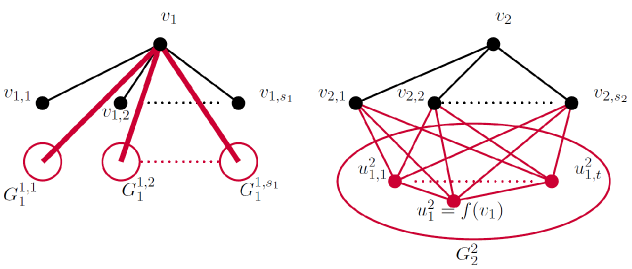
Figure 4: A piece of neighbourhood corona of $G_{1}$ and $G_{2}$ in the proof of Lemma 2.4.

Since $f$ preserves the adjacency relation, so $f(N_{G_{1}\star G_{2}}(v_{1}))=N_{G_{1}\star G_{2}}(u_{1}^{2})$, i.e.,

$$\big{\{}f(v_{1,1}),\ldots,f(v_{1,s_{1}}),f(u_{1}^{1,1}),\ldots,f(u_{n_{2}}^{1,1}), \ldots,f(u_{1}^{1,s_{1}}),\ldots,f(u_{n_{2}}^{1,s_{1}})\big{\}}$$

$$=\{u_{1,1}^{2},\ldots,u_{1,t}^{2},v_{2,1},\ldots,v_{2,s_{2}}\}.$$ (4)

Since $t<n_{2}$, there are vertices in the copies $G_{2}^{1,1},\ldots,G_{2}^{1,s_{1}}$ such that they are mapped to the elements of the set $\{v_{2,1},\ldots,v_{2,s_{2}}\}$, under the automorphism $f$. Without loss of generality we can assume that $f(u_{i_{j}}^{1,j})=v_{2,j}$, where $1\leqslant j\leqslant s_{1}$. We continue the proof by considering two cases for $s_{1}$ as follows:

Case 1) If $s_{1}>1$. Since $v_{2}$ is adjacent to the vertices $v_{2,1},\ldots,v_{2,s_{1}}$, so $f^{-1}(v_{2})$ is adjacent to the vertices $u_{i_{1}}^{1,1},\ldots,u_{i_{s_{1}}}^{1,s_{1}}$. Since $s_{1}>1$, so $f^{-1}(v_{2})\in G_{1}$ and $f^{-1}(v_{2})$ is adjacent to the vertices $v_{1,1},\ldots,v_{1,s_{1}}$. Hence $v_{2}$ is adjacent to the vertices $f(v_{1,1}),\ldots,f(v_{1,s_{1}})$, and by Equation 2 we have

$$\{f(v_{1,1}),\ldots,f(v_{1,s_{1}})\}\subseteq\{v_{2,s_{1}+1},\ldots,v_{2,s_{2}}\}.$$ (5)

Without loss of generality we assume that $f(v_{1,i})=v_{2,s_{1}+i}$, where $1\leqslant i\leqslant s_{1}$ (see Figure 5).

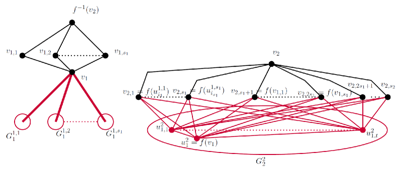
Figure 5: A piece of neighbourhood corona of $G_{1}$ and $G_{2}$ in the proof of Lemma 2.4.

Since $f^{-1}(v_{2})$ is adjacent to the vertices $v_{1,1},\ldots,v_{1,s_{1}}$, we can say that $f^{-1}(v_{2})$ is adjacent to all vertices of $G_{2}^{1,1},\ldots,G_{2}^{1,s_{1}}$, so $v_{2}$ is adjacent to all vertices of $f(G_{2}^{1,1}),\ldots,f(G_{2}^{1,s_{1}})$. Then by Equation (2) we get

$$\{f(u_{1}^{1,1}),\ldots,f(u_{n_{2}}^{1,1}),\ldots,f(u_{1}^{1,s_{1}}),\ldots,f(u_{n_{2}}^{1,s_{1}})\}\subseteq\{v_{2,1},\ldots,v_{2,s_{2}}\}.$$ (6)

With respect to Equations (2), (5) and (6) we have a contradiction.

Case 2) If $s_{1}=1$. Since $f$ preserves the adjacency relation, so

$$\{f(v_{1,1}),f(u_{1}^{1,1}),\ldots,f(u_{n_{2}}^{1,1})\}=\{u_{1,1}^{2},\ldots,u_{1,t}^{2},v_{2,1},\ldots,v_{2,s_{2}}\}.$$ (7)

Since $t<n_{2}$, there exists a vertex in the copy $G_{2}^{1,1}$ such that it is mapped to an elements of the set $\{v_{2,1},\ldots,v_{2,s_{2}}\}$, under the automorphism $f$. Without loss of generality we can assume that $f(u_{i_{1}}^{1,1})=v_{2,1}$. Since $v_{2}$ is adjacent to $v_{2,1}$, so $f^{-1}(v_{2})$ is adjacent to $u_{i_{1}}^{1,1}$, and since $f^{-1}(v_{2})\neq v_{1}$, so $f^{-1}(v_{2})\in G_{2}^{1,1}$. Without loss of generality we can assume that $f^{-1}(v_{2})=u_{i_{1}1}^{1,1}$ such that $u_{i_{1}1}^{1,1}$ is adjacent to $u_{i_{1}}^{1,1}$ (see Figure 6).

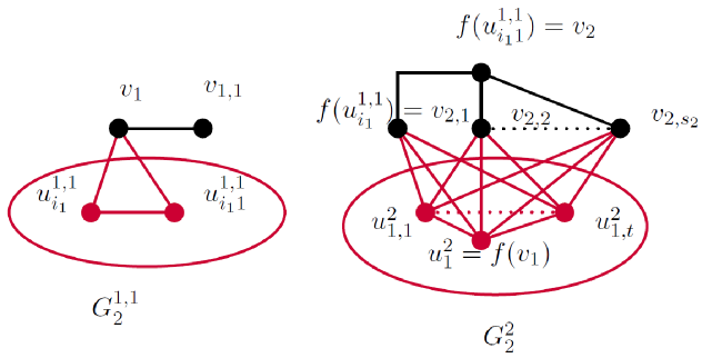
Figure 6: A piece of neighbourhood corona of $G_{1}$ and $G_{2}$ in the proof of Lemma 2.4.

Since $v_{1,1}$ is adjacent to the vertex $v_{1}$ and $dist_{G_{1}\star G_{2}}(v_{1,1},u_{i_{1}}^{1,1})=dist_{G_{1}\star G_{2}}(v_{1,1},u_{i_{1}1}^{1,1})=2$, so $f(v_{1,1})$ is adjacent to the vertex $u_{1}^{2}$ and also

$$dist_{G_{1}\star G_{2}}(f(v_{1,1}),v_{2})=dist_{G_{1}\star G_{2}}(f(v_{1,1}),v_{2,1})=2.$$ (8)

Now by Equations (7) and (8) we have a contradiction. Therefore the restriction of each automorphism of $G_{1}\star G_{2}$ to $G_{1}$ is an automorphism of $G_{1}$. $\square$

Corollary 2.5

Let $G_{1}$ and $G_{2}$ be two connected graphs of order $n_{1}$ and $n_{2}$, respectively, such that $n_{1}>1$ and $f$ is an automorphism of $G_{1}\star G_{2}$. Then the restriction of $f$ to $G_{1}$ is an automorphism of $G_{1}$ and also there are the automorphism $g$ of $G_{1}$ and the automorphisms $h_{1},\ldots,h_{n_{1}}$ of $G_{2}$ such that $f(G_{2}^{i})=(h_{i}(G_{2}))^{k}$, where $v_{k}=g(v_{i})$ and $i,k=1,\ldots,n_{1}$.

Proof. By Lemmas 2.3 and 2.4, it is sufficient to prove that the copies of $G_{2}$ are mapped to each other under the automorphism $f$, and it follows from that $f$ preserves the adjacency relation on each copy of $G_{2}$. $\square$

The following corollary is an immediate consequence of Corollary 2.5 for graphs of the form $G\star K_{1}$.

Corollary 2.6

Let $G$ be a connected graph of order $n>1$ and $f$ be an arbitrary automorphism of $G\star K_{1}$. Then the restriction of $f$ to $G$ is an automorphism of $G$. Also $f(K_{1}^{i})=K_{1}^{j_{i}}$ for some automorphism $g$ of $G$ such that $g(v_{i})=v_{j_{i}}$ where $i,j_{i}=1,2,\ldots,n_{1}$.

3 Study of $D(G_{1}\star G_{2})$ and $D^{\prime}(G_{1}\star G_{2})$

In this section we use the results in Section 2 to study the distinguishing number and the distinguishing index of the neighbourhood corona of two graphs. First we consider the neighbourhood corona of an arbitrary graph with $K_{1}$. The following theorem gives an upper bound for $D(G\star K_{1})$ and $D^{\prime}(G\star K_{1})$.

Theorem 3.1

Let $G$ be a connected graph of order $n>1$. We have

• $D(G\star K_{1})\leqslant D(G)$,

• $D^{\prime}(G\star K_{1})\leqslant D^{\prime}(G)$.

Proof.

1. We shall define a distinguishing vertex labeling for $G\star K_{1}$ with $D(G)$ labels. First we label $G$ in a distinguishing way with $D(G)$ labels. Next we assign the vertex $K_{1}^{v_{i}}$, the label of the vertex $v_{i}$ where $1\leqslant i\leqslant n$. This labeling is a distinguishing vertex labeling of $G\star K_{1}$, because if $f$ is an automorphism of $G\star K_{1}$ preserving the labeling then by Corollary 2.5, the restriction of $f$ to $G$ is an automorphism of $G$ preserving the labeling. Since we labeled $G$ in a distinguishing way at first, so the restriction of $f$ to $G$ is the identity automorphism on $G$. On the other hand by Corollary 2.6 there exists an automorphism $g$ of $G$ such that $f(K_{1}^{v_{i}})=K_{1}^{g(v_{i})}$, $1\leqslant i\leqslant n$. Regarding to the labeling of copies of $K_{1}$, we can obtain that $g$ is the identity automorphism on $G$, and so $f$ is the identity automorphism on $G\star K_{1}$.

2. We define a distinguishing edge labeling for $G\star K_{1}$ with $D^{\prime}(G)$ labels. First we label the edges of $G$ in a distinguishing way with $D^{\prime}(G)$ labels. By Equations (1) and (2) we know that the degree of $K_{1}^{v_{i}}$ in $G\star K_{1}$ is equal with the degree of $v_{i}$ in $G$ where $1\leqslant i\leqslant n$. Now we assign the edge between $K_{1}^{v_{i}}$ and $v_{i,j}$ where $v_{i,j}\in N_{G}(v_{i})$, the label of the edges between $v_{i}$ and $v_{i,j}$ where $j=1,\ldots,d_{G}(v_{i})$. This labeling is a distinguishing edge labeling of $G\star K_{1}$, because if $f$ is an automorphism of $G\star K_{1}$ preserving the labeling then by Corollary 2.5, the restriction of $f$ to $G$ is an automorphism of $G$ preserving the labeling. Since we labeled $G$ in a distinguishing way at first, so the restriction of $f$ to $G$ is the identity automorphism on $G$. On the other hand by Corollary 2.6 there exists an automorphism $g$ of $G$ such that $f(K_{1}^{v_{i}})=K_{1}^{g(v_{i})}$, $1\leqslant i\leqslant n$. Regarding to the labeling of the edges incident to each copies of $K_{1}$, we can obtain that $g$ is the identity automorphism on $G$, and so $f$ is the identity automorphism on $G\star K_{1}$. $\square$

The bounds of $D(G\star K_{1})$ and $D^{\prime}(G\star K_{1})$ in Theorem 3.1 are sharp. If we consider $G$ as the star graph $K_{1,n}$, $n>1$, then $K_{1,n}\star K_{1}$ is a graph as shown in Figure 7. Using the degree of the verices of $K_{1,n}\star K_{1}$ we can get the automorphism group of $K_{1,n}\star K_{1}$ and then it can be concluded that $D(K_{1,n}\star K_{1})=n=D(K_{1,n})$, and also $D^{\prime}(K_{1,n}\star K_{1})=n=D^{\prime}(K_{1,n})$.

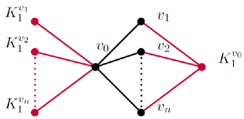
Figure 7: The neighbourhood corona of $K_{1,n}$ and $K_{1}$.

In Theorem 3.1, the sharp upper bounds for $D(G\star K_{1})$ and $D^{\prime}(G\star K_{1})$ have been given, but we did not present lower bounds for these parameters. Actually, there are graphs whose distinguishing number can be arbitrarily larger than the distinguishing number of its neighbourhood corona with $K_{1}$. In other words, we can show that there exists a connected graph $G$ of order $n>1$ such that the value of $\frac{D(G\star K_{1})}{D(G)}$ can be arbitrarily small. To do this we need the two following theorems. Recall that the friendship graph $F_{n}$ $(n\geqslant 2)$ can be constructed by joining $n$ copies of the cycle graph $C_{3}$ with a common vertex.

Theorem 3.2

[2] The distinguishing number of the friendship graph $F_{n}$ $(n\geq 2)$ is

$$D(F_{n})=\big{\lceil}\frac{1+\sqrt{8n+1}}{2}\big{\rceil}.$$

Now we obtain the exact value of the distinguishing number of neighborhood corona of $F_{n}$ with $K_{1}$.

Theorem 3.3

The distinguishing number of $F_{n}\star K_{1}$ $(n\geq 2)$ is

$$D(F_{n}\star K_{1})=\big{\lceil}\sqrt{\dfrac{1+\sqrt{8n+1}}{2}}\big{\rceil}.$$

Proof. Let $V(F_{n})=\{v_{0},v_{1},v_{2},\ldots,v_{2n-1},v_{2n}\}$ and the vertex $v_{0}$ be the central vertex and $v_{2i-1}$ and $v_{2i}$ be the vertices of the base of triangles in $F_{n}$ where $1\leqslant i\leqslant n$. So $d_{F_{n}}(v_{0})=2n$ and $d_{F_{n}}(v_{i})=2$ where $1\leqslant i\leqslant 2n$. By Equations (1) and (2) we have $d_{F_{n}\star K_{1}}(v_{0})=4n$ and $d_{F_{n}\star K_{1}}(v_{i})=4$, also $d_{F_{n}\star K_{1}}(K_{1}^{v_{0}})=2n$ and $d_{F_{n}\star K_{1}}(K_{1}^{v_{i}})=2$ where $1\leqslant i\leqslant 2n$ (see Figure 8).

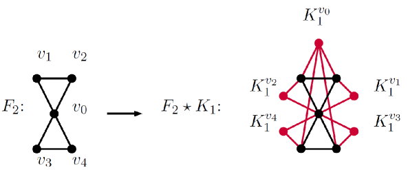
Figure 8: The graphs $F_{2}$ and $F_{2}\star K_{1}$.

If $f$ is an automorphism of $F_{n}\star K_{1}$, then $f$ fixes the vertices $v_{0}$ and $K_{1}^{v_{0}}$ (if $n=2$ we can get the same result by Corollary 2.5). So we assign the vertices $v_{0}$ and $K_{1}^{v_{0}}$ the label $1$. Let $(x_{i},y_{i},z_{i},w_{i})$ be the label of the vertices $(K_{1}^{v_{2i}},v_{2i-1},v_{2i},K_{1}^{v_{2i-1}})$ where $1\leqslant i\leqslant n$. Suppose that $L=\{(x_{i},y_{i},z_{i},w_{i})~{}|~{}1\leqslant i\leqslant n,x_{i},y_{i},z_{i},w_{i}\in\mathbb{N}\}$, is a labeling of the vertices of $F_{n}\star K_{1}$ except the vertices $v_{0}$ and $K_{1}^{v_{0}}$. If $L$ is a distinguishing labeling of $F_{n}\star K_{1}$ then:

• For every $i=1,\ldots,n$, it should be satisfied that $x_{i}\neq w_{i}$ or $y_{i}\neq z_{i}$. Otherwise, the automorphism $f_{i}$ of $F_{n}\star K_{1}$ such that $f_{i}$ maps $K_{1}^{v_{2i}}$ and $K_{1}^{v_{2i-1}}$ to each other, two vertices $v_{2i-1}$ and $v_{2i}$ to each other, and fixes the remaining vertices, preserves the labeling.

• For every $i$ and $j$ in $\{1,\ldots,n\}$, with $i\neq j$, it should be satisfied that $(x_{i},y_{i},z_{i},w_{i})\neq(x_{j},y_{j},z_{j},w_{j})$ and $(x_{i},y_{i},z_{i},w_{i})\neq(w_{j},z_{j},y_{j},x_{j})$. Otherwise, the automorphism $f_{ij}$ and $g_{ij}$ of $F_{n}\star K_{1}$ by the following definitions preserve the labeling.

• The automorphism $f_{ij}$ maps $K_{1}^{v_{2i}}$ and $K_{1}^{v_{2j}}$ to each other and also $K_{1}^{v_{2i-1}}$ and $K_{1}^{v_{2j-1}}$ to each other. The map $f_{ij}$ maps $v_{2i}$ and $v_{2j}$ to each other, also it maps $v_{2i-1}$ and $v_{2j-1}$ to each other and fixes the remaining vertices of $F_{n}\star K_{1}$.

• The automorphism $g_{ij}$ maps $K_{1}^{v_{2i}}$ and $K_{1}^{v_{2j-1}}$ to each other, also $K_{1}^{v_{2i-1}}$ and $K_{1}^{v_{2j}}$ to each other. The map $g_{ij}$ maps $v_{2i}$ and $v_{2j-1}$ to each other, also it maps $v_{2i-1}$ and $v_{2j}$ to each other and fixes the remaining vertices of $F_{n}\star K_{1}$.

So using the label set $\{1,\ldots,s\}$ we can make at most $(s^{4}-s^{2})/2$ of the $4$-ary’s $(x,y,z,w)$ satisfying $(i)$ and $(ii)$. Because, the number of $4$-ary’s $(x,y,z,w)$ such that $x\neq w$ is $s(s-1)s^{2}$, and the number of $4$-ary’s $(x,y,z,w)$ such that $y\neq z$ is $s(s-1)s^{2}$. On the other hand the number of $4$-ary’s $(x,y,z,w)$ such that $x\neq w$ and $y\neq z$ is $(s(s-1))^{2}$. So the maximum number of $4$-ary’s $(x,y,z,w)$ satisfying $(i)$ is

$$(s(s-1)s^{2}+s(s-1)s^{2})-(s(s-1))^{2}=s^{4}-s^{2}.$$

Among these $4$-ary’s we should choose the $4$-ary’s that satisfying $(ii)$, too. Therefore the number of $4$-ary’s $(x,y,z,w)$ satisfying $(i)$ and $(ii)$ which they can make by the label set $\{1,\ldots,s\}$ is $\frac{s^{4}-s^{2}}{2}$. Therefore $D(F_{n}\star K_{1})\geqslant min\{s:\frac{s^{4}-s^{2}}{2}\geqslant n\}$. By an easy computation, we see that

$$min\{s:\frac{s^{4}-s^{2}}{2}\geqslant n\}=\lceil\sqrt{\dfrac{1+\sqrt{8n+1}}{2}}\rceil.$$

Now we present a distinguishing vertex labeling with this number of labels. We assign $v_{0}$ and $K_{1}^{v_{0}}$ the label $1$. We should label the remaining vertices such that the identity automorphism preserves the labeling only. Denoting each pentagon with the vertices $K_{1}^{v_{2i}},v_{2i-1},v_{2i},K_{1}^{v_{2i-1}},v_{0}$ in $F_{n}\star K_{1}$ where $1\leqslant i\leqslant n$, by a general pentagon that have shown in Figure 9 and calling it a blade and continue the labeling.

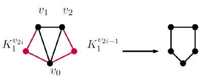
Figure 9: The considered pentagon (or a cycle of size $5$) in the proof of Theorem 3.3.

At first, we want to know the maximum number of blades that can be labeled in a distinguishing way by $1$ and $2$. As we can see in Figure 10, the maximum number of blades that can be labeled in distinguishing way, by $1,2$ is $\underline{6}$.

In order to preserve the labeling under the identity automorphism only, we should use another label to assign the next blade. As mentioned earlier, the maximum number of blades that can be labeled by each the set $\{1,3\},\{2,3\}$ is six. Now we want to know the maximum number of blades that can be labeled by presence of $\{1,2,3\}$ at the same time in the blade. This number is $18$. Because let to label with the labels $1,2,3$ and a repetition of $1$. As shown in Figure 10, we can label six blades. Obviously we can do the same with letting repetition of $2$ and $3$. Therefore the maximum number of blades that can be labeled by presence of $\{1,2,3\}$ at the same time is $\underline{18}$. Until now, we labeled $36$ blades.

$$\underbrace{6}_{\{1,2\}}+\underbrace{6}_{\{1,3\}}+\underbrace{6}_{\{2,3\}}+\underbrace{18}_{\{1,2,3\}}=36$$

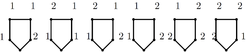
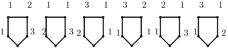
Figure 10: Distinguishing labeling of blades with the labels $\{1,2\}$ and $\{1,2,3\}$, respectively.

If we want to label the next blade, we should add a new label, $4$. The maximum number of blades that can be labeled by each the set $\{1,4\},\{2,4\},\{3,4\}$ is six. Also, the maximum number of blades that can be labeled by each the set $\{1,2,4\},\{1,3,4\},\{2,3,4\}$ is eighteen. We can see that the maximum number of blades that can be labeled by presence of $\{1,2,3,4\}$ at the same time is $\underline{12}$ as Shown in Figure 11.

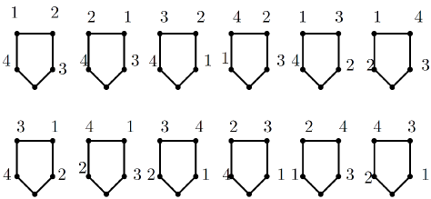
Figure 11: The distinguishing labeling of blades with the labels $\{1,2,3,4\}$.

Thus we have labeled $120$ blades until now.

$$36+\underbrace{6}_{\{1,4\}}+\underbrace{6}_{\{2,4\}}+\underbrace{6}_{\{2,4\}}+\underbrace{18}_{\{1,2,4\}}+\underbrace{18}_{\{1,3,4\}}+\underbrace{18}_{\{2,3,4\}}+\underbrace{12}_{\{1,2,3,4\}}=120.$$

Therefore the relationship between the number of labels that has been used, $\mathbf{d}(F_{n}\star K_{1})$, and $n$ are as the following sequence:

$$\{\mathbf{d}(F_{n}\star K_{1})\}=\{0,\underbrace{2}_{6-times},\underbrace{3}_{30-times},\underbrace{4}_{84-times},\ldots,m,\ldots,m,\ldots\}.$$

where the number of the repetitions $m$ in above sequence is $(m-1)6+{m-1\choose 2}18+{m-1\choose 3}12$, with $m\geqslant 1$.

In fact, $\mathbf{d}(F_{n}\star K_{1})=min\{k:~{}\sum_{i=1}^{k}\left({i-1\choose 1}6+{m-1\choose 2}18+{m-1\choose 3}12\right)\geqslant n\}$. By an easy computation, we see that

$$min\{k:~{}\sum_{i=1}^{k}\left({i-1\choose 1}6+{m-1\choose 2}18+{m-1\choose 3}12\right)\geqslant n\}$$

$$=min\{k:(k^{4}-k^{2})/2\geqslant n\}$$

$$=\lceil\sqrt{\dfrac{1+\sqrt{8n+1}}{2}}\rceil.$$

Therefore we have the result. $\square$

Now we are ready to state and prove the following theorem:

Theorem 3.4

There exists a connected graph $G$ of order $n>1$ such that the value of $\frac{D(G\star K_{1})}{D(G)}$ can be arbitrarily small.

Proof. By Theorems 3.2 and 3.3 it can be seen that

$$lim_{n\rightarrow\infty}\dfrac{D(F_{n}\star K_{1})}{D(F_{n})}=lim_{n\rightarrow\infty}\dfrac{\lceil\sqrt{\dfrac{1+\sqrt{8n+1}}{2}}\rceil}{\lceil\dfrac{1+\sqrt{8n+1}}{2}\rceil}=0$$

Therefore we have the result. $\square$

The following theorem is one of the main result of this paper and gives an upper bound for the distinguishing number of the neighbourhood corona of two arbitrary graphs:

Theorem 3.5

Let $G_{1}$ and $G_{2}$ be two connected graphs of orders $n_{1}$ and $n_{2}$, respectively, such that $n_{1}>1$. Then $D(G_{1}\star G_{2})\leqslant max\{D(G_{1}),D(G_{2})+M\}$, where

$$M=min\left\{k:\sum_{m=0}^{k}y_{m}\geqslant D(G_{1})\right\},~{}~{}~{}y_{m}=\left\{\begin{array}[]{ll}1&m=0,\\ D(G_{2})&m=1,\\ D(G_{2})+\sum_{i=1}^{m-1}{m-1\choose i}{D(G_{2})\choose i+1}&m\geqslant 2.\end{array}\right.$$

Proof. We define a distinguishing vertex labeling for $G_{1}\star G_{2}$ with $max\{D(G_{1}),D(G_{2})+M\}$ labels. First we label $G_{1}$ with $D(G_{1})$ labels in a distinguishing way. For the labeling of copies of $G_{2}$, we partition the vertices of $G_{1}$ by the distinguishing labeling of $G_{1}$, i.e., we partition the vertices of $G_{1}$ into $D(G_{1})$ classes, such that $[i]$th class contains the vertices of $G_{1}$ having the label $i$, in the distinguishing labeling of $G_{1}$, where $1\leqslant i\leqslant D(G_{1})$. Let $[i]=\{v_{i1},\ldots,v_{is_{i}}\}$, where $s_{i}$ is the size of $[i]$th class and $1\leqslant i\leqslant D(G_{1})$. By this partition we label the copies of $G_{2}$ as follows: First we label the vertices of $G_{2}$ with $D(G_{2})$ labels in a distinguishing way, next we do the following changes on the labeling of $G_{2}$. Before the labeling of the copies of $G_{2}$, we introduce the notation $G_{2}^{[i]}$ for the set $\{G_{2}^{i1},\ldots,G_{2}^{is_{i}}\}$, i.e., $G_{2}^{[i]}$ is the set of that copies of $G_{2}$ corresponding to the elements of $[i]$th class, where $1\leqslant i\leqslant D(G_{1})$. In fact we partition the copies of $G_{2}$ into $D(G_{1})$ classes, that $G_{2}^{[i]}$ is the notation of $[i]$th class. Now we present the labeling of copies of $G_{2}$ by the following steps:

Step 1) We label all of the copies of $G_{2}$ which are in $G_{2}^{[1]}$, exactly the same as the distinguishing labeling of $G_{2}$.

Step 2) For the labeling of the copies in $G_{2}^{[i]}$, where $2\leqslant i\leqslant D(G_{2})+1$, we use of the new label $D(G_{2})+1$ in such a way that the label $i-1$ in the all elements of $G_{2}^{[i]}$ is replaced by the new label $D(G_{2})+1$, where $2\leqslant i\leqslant D(G_{2})+1$.

Step 3) For the labeling of the copies in $G_{2}^{[i]}$, where $D(G_{2})+2\leqslant i\leqslant 2D(G_{2})+1$, we do the same action as Step 2, with the new label $D(G_{2})+2$, instead of the labels $D(G_{2})+1$.

Step 4) By choosing two labels among the labels $\{1,\ldots,D(G_{2})\}$, and replacing them by the two new labels $D(G_{2})+1$ and $D(G_{2})+2$, we can label the elements of ${D(G_{2})\choose 2}$ other classes of the classes $G_{2}^{[i]}$.

Step 5) We do the same work as Step 2 with the new label $D(G_{2})+3$ instead of labels $D(G_{2})+1$. Next we label $2{D(G_{2})\choose 2}$ other classes $G_{2}^{[i]}$, with the two new labels $D(G_{2})+1$ and $D(G_{2})+3$, also with the labels $D(G_{2})+2$ and $D(G_{2})+3$, exactly the same as Step 4.

Step 6) Now we choose three labels among the labels $\{1,\ldots,D(G_{2})\}$, and replace them by the three new labels $D(G_{2})+1$, $D(G_{2})+2$ and $D(G_{2})+3$.

By continuing this method we conclude that the number of classes can be labeled with the labels $1,\ldots,D(G_{2})+m$, $m\geqslant 1$, such that the label $D(G_{2})+m$ is used in the labeling of each element of classes, is $y_{m}$ where

$$y_{m}=\left\{\begin{array}[]{ll}1&m=0,\\ D(G_{2})&m=1,\\ D(G_{2})+\sum_{i=1}^{m-1}{m-1\choose i}{D(G_{2})\choose i+1}&m\geqslant 2.\end{array}\right.$$

Therefore the number of labels that have been used for the labeling of all copies of $G_{2}$, is $D(G_{2})+M$ where $M=min\left\{k:\sum_{m=0}^{k}y_{m}\geqslant D(G_{1})\right\}$. This labeling is a distinguishing vertex labeling of $G_{1}\star G_{2}$, because if $f$ is an automorphism of $G_{1}\star G_{2}$ preserving the labeling, then by Corollary 2.5, $f|_{G_{1}}$ is an automorphism of $G_{1}$ preserving the labeling. Since we labeled $G_{1}$ in a distinguishing way, at first, so $f$ is the identity automorphism on $G_{1}$. Regarding to the labeling of copies of $G_{2}$ and since $f$ preserves the labeling of the copies of $G_{2}$, so $f$ maps each copy of $G_{2}$ to itself. The map $f$ is the identity automorphism on each copy of $G_{2}$, because each copy of $G_{2}$ was labeled in a distinguishing way. Therefore $f$ is the identity automorphism on $G_{1}\star G_{2}$. $\square$

The following corollary is an immediate consequence of Theorem 3.5.

Corollary 3.6

Let $G_{1}$ and $G_{2}$ be two connected graphs of orders $n_{1}$ and $n_{2}$, respectively, such that $n_{1}>1$. If $D(G_{1})=1$, then $D(G_{1}\star G_{2})\leqslant D(G_{2})$.

Proof. It is sufficient to note that if $D(G_{1})=1$, then the value of $M$ in Theorem 3.5 is zero. $\square$

We end the paper by presenting an upper bound for the distinguishing index of the neighbourhood corona of two graphs:

Theorem 3.7

Let $G_{1}$ and $G_{2}$ be two connected graphs of orders $n_{1}$ and $n_{2}$, respectively, such that $n_{1}>1$. Then $D^{\prime}(G_{1}\star G_{2})\leqslant max\{D^{\prime}(G_{1}),D^{\prime}(G_{2})\}$.

Proof. We define an edge distinguishing labeling of $G_{1}\star G_{2}$ with $max\{D^{\prime}(G_{1}),D^{\prime}(G_{2})\}$ labels. To obtain such labeling we first label the edge set of $G_{1}$ and $G_{2}$ in a distinguishing way with $D^{\prime}(G_{1})$ and $D^{\prime}(G_{2})$ labels, respectively. For the labeling of the edges between each copy of $G_{2}$ and $G_{1}$ we use of the labeling of the edge set of $G_{1}$ as follows:

Let $N_{G_{1}}(v_{k})=\{v_{k1},\ldots,v_{1|N_{G_{1}}(v_{k})|}\}$, where $1\leqslant k\leqslant n_{1}$. By the notations of the vertices of $G_{1}$ and the copies of $G_{2}$, we assign the all edges $v_{kj_{k}}u_{i}^{k}$, $1\leqslant i\leqslant n_{2}$, the label of the edge $v_{kj_{k}}v_{k}$ in the distinguishing labeling of the edge set of $G_{1}$, where $1\leqslant k\leqslant n_{1}$ and $1\leqslant j_{k}\leqslant|N_{G_{1}}(v_{k})|$. This labeling is a distinguishing edge labeling of $G_{1}\star G_{2}$, because if $f$ is an automorphism of $G_{1}\star G_{2}$ preserving the labeling, then by Corollary 2.5, the restriction of $f$ to $G_{1}$ is an automorphism of $G_{1}$ preserving the labeling. Since we labeled $G_{1}$ in a distinguishing way, at first, so $f$ is the identity automorphism on $G_{1}$. Regarding to the labeling of the edges between the copies of $G_{2}$ and $G_{1}$ and by Corollary 2.5 we conclude that $f$ maps each copy of $G_{2}$ to itself. Since we labeled each copy of $G_{2}$ in a distinguishing way, at first, so the map $f$ is the identity automorphism on each copy of $G_{2}$, and so $f$ is the identity automorphism on $G_{1}\star G_{2}$. $\square$

References

[1] M.O. Albertson and K.L. Collins, Symmetry breaking in graphs, Electron. J. Combin. 3 (1996) #R18.
[2] S. Alikhani and S. Soltani, Distinguishing number and distinguishing index of certain graphs, submitted. Available at http://arxiv.org/abs/1602.03302.
[3] R. Frucht and F. Harary, On the corona two graphs, Aequationes Math. 4 (1970) 322-325.
[4] F. Harary, Graph Theory, Addition-Wesley Publishing Co., Reading, MA/Menlo Park, CA/London, 1969.
[5] I. Gopalapillai, The spectrum of neighborhood corona of graphs, Kragujevac Journal of Mathematics. 35 (2011) 493-500.
[6] R. Kalinowski and M. Pilsniak, Distinguishing graphs by edge colourings, European J. Combin. 45 (2015) 124-131.
[7] S. Klav̌zar and X. Zhu, Cartesian powers of graphs can be distinguished by two labels, European J. Combin. 28 (2007) 303-310.
[8] X. Liu and S. Zhou, Spectra of the neighbourhood corona of two graphs, Linear Multilinear Alg. 62, 9 (2014) 1205–1219.
[9] F. Michael and I. Garth, Distinguishing colorings of Cartesian products of complete graphs, Discrete Math., 308 (11), (2008) 2240-2246.
[10] E. Sampathkumar, H. B. Walikar, On the splitting graph of a graph, Karnatak Univ. J. Sci. 35/36 (1980-1981), 13-16.