Generalized Volterra lattices:
binary Darboux transformations and self-consistent sources

Abstract

We study two families of matrix versions of generalized Volterra (or Bogoyavlensky) lattice equations. For each family, the equations arise as reductions of a partial differential-difference equation in one continuous and two discrete variables, which is a realization of a general integrable equation in bidifferential calculus. This allows to derive a binary Darboux transformation and also self-consistent source extensions via general results of bidifferential calculus. Exact solutions are constructed from the simplest seed solutions.

1 Introduction

The famous Volterra lattice equation [1, 2, 3, 4, 5, 6] is

$$V_{t}=V\,V_{(1)}-V_{(-1)}\,V\,,$$ (1.1)

here generalized to a matrix variable $V$. $V_{t}$ denotes the derivative of $V$ with respect to the continuous variable $t$, and $V_{(\pm 1)}$ are the values at the adjacent lattice sites. (1.1) is a member of the family

$$(VV_{(1)}\cdots V_{(k-1)})_{t}=\left\{\begin{array}[]{l}V\cdots V_{(l-1)}-V_{(k-l)}\cdots V_{(k-1)}\\ V_{(-1)}^{-1}\cdots V_{(l)}^{-1}-V_{(k-l-1)}^{-1}\cdots V_{(k)}^{-1}\end{array}\right.\,\mbox{if}\;\begin{array}[]{l}l>0\\ l<0\end{array}$$ (1.6)

of generalized Volterra lattice equations. Here $k>0$ and $l$ are integers and we recover (1.1) for $k=1$ and $l=2$. The family of equations (1.6) has been explored, mostly only in the scalar case, in [7, 8, 9, 10, 11, 12, 13, 14, 15, 16, 17, 18, 19, 20], for example. For $k=1$ and $l=-1$, (1.6) yields the modified Volterra lattice equation

$$U_{t}=U\,(U_{(1)}-U_{(-1)})\,U$$ (1.7)

in terms of $U=V^{-1}$. In Section 2 we show that there is an integrable semi-discrete chiral model (see (2.15)), for an invertible matrix variable $g$ depending on one continuous and two discrete variables, which admits the reductions

$$(g\,g_{(k)}^{-1})_{t}=g\,g_{(l)}^{-1}-(g\,g_{(l)}^{-1})_{(k-l)}\,.$$ (1.8)

Via

$$V=g\,g_{(1)}^{-1}\,,$$ (1.9)

(1.8) implies the corresponding generalized Volterra lattice equation (1.6).

Using the framework of bidifferential calculus [21, 22], we construct binary Darboux transformations for the above mentioned semi-discrete chiral model and its reductions (1.8). Moreover, we derive self-consistent source extensions (see the references cited in [23]) of these equations, following the general construction developed in [23]. We also refer to the latter publication for a representative list of references concerning this way of extending an integrable equation to an equation with additional “source terms”, which involve new dependent variables governed by equations that also involve the variable of the original equation.

A second family of equations generalizing the Volterra lattice equation is given by

$$\Big{(}\sum_{i=0}^{k-1}W_{(i)}\Big{)}_{t}=\sum_{i=0}^{l-1}W_{(i)}\sum_{i=0}^{k-1}W_{(i)}-\sum_{i=0}^{k-1}W_{(i)}\sum_{i=k-l}^{k-1}W_{(i)}\,.$$ (1.10)

Such equations have been explored in [25, 8, 9, 10, 11, 26, 15, 17, 27], mostly in the scalar case. For $k=1$ this reduces to

$$W_{t}=\sum_{i=1}^{l-1}W_{(i)}\,W-W\,\sum_{i=1}^{l-1}W_{(-i)}\,,$$

which for $l=2$ is the Volterra lattice equation in the form $W_{t}=W_{(1)}W-WW_{(-1)}$. There is a differential-difference equation (see (3.78)), for a variable $\varphi$ depending on one continuous and two discrete variables, which admits reductions to

$$(\varphi_{(k)}-\varphi)_{t}=(\varphi_{(l)}-\varphi)(\varphi_{(k)}-\varphi+I)-(\varphi_{(k)}-\varphi+I)(\varphi_{(l)}-\varphi)_{(k-l)}\,,$$ (1.11)

where $I$ is the identity matrix, and we observe that, in terms of

$$W=\varphi_{,1}-\varphi+\frac{1}{k}\,I\,,$$ (1.12)

the latter becomes (1.10). Using results of [23], in the framework of bidifferential calculus, we construct binary Darboux transformations and self-consistent source extensions for these equations.

The equations (1.6) and (1.10), for $k=1$, are also known as Bogoyavlensky lattices (cf. [17]).

In Section 2 we present a bidifferential calculus formulation for the semi-discrete chiral model. Section 2.1 recalls from [23] some general results concerning binary Darboux transformations and self-consistent source extensions of integrable equations in this framework. In Section 2.2 we derive self-consistent source extensions of the semi-discrete chiral model equation and construct corresponding exact solutions. In Section 2.3 we derive self-consistent source extensions of the first family of generalized Volterra lattice equations as reductions of the self-consistent source extensions of the semi-discrete chiral model. We also present infinite families of exact solutions of these equations. Section 3 contains a corresponding treatment of the second family of generalized Volterra lattice equations. Section 4 contains some concluding remarks.

2 An integrable semi-discrete chiral model and the first family of generalized Volterra lattices

Let $\boldsymbol{\Omega}=\bigoplus_{r\geq 0}\boldsymbol{\Omega}^{r}$ be an associative unital graded algebra over $\mathbb{C}$. In particular, $\mathcal{A}:=\boldsymbol{\Omega}^{0}$ is an associative unital algebra over $\mathbb{C}$ and $\boldsymbol{\Omega}^{r}$, $r\geq 1$, are $\mathcal{A}$-bimodules such that $\boldsymbol{\Omega}^{r}\,\boldsymbol{\Omega}^{s}\subseteq\boldsymbol{\Omega}^{r+s}$. A bidifferential calculus is an associative unital graded algebra $\boldsymbol{\Omega}$, supplied with two $\mathbb{C}$-linear, graded derivations $\mathrm{d},\bar{\mathrm{d}}:\boldsymbol{\Omega}\rightarrow\boldsymbol{\Omega}$ of degree one (hence $\mathrm{d}\boldsymbol{\Omega}^{r}\subseteq\boldsymbol{\Omega}^{r+1}$, $\bar{\mathrm{d}}\boldsymbol{\Omega}^{r}\subseteq\boldsymbol{\Omega}^{r+1}$), and such that $\mathrm{d}^{2}=\bar{\mathrm{d}}^{2}=\mathrm{d}\bar{\mathrm{d}}+\bar{\mathrm{d}}\mathrm{d}=0$. In this work we choose, as in [23], the graded algebra $\boldsymbol{\Omega}$ to be of the form $\boldsymbol{\Omega}=\mathcal{A}\otimes\boldsymbol{\Lambda}$ with the exterior (Grassmann) algebra $\boldsymbol{\Lambda}=\bigoplus_{i=0}^{2}\boldsymbol{\Lambda}^{i}$ of the vector space $\mathbb{C}^{2}$. It is then sufficient to define $\mathrm{d}$ and $\bar{\mathrm{d}}$ on $\mathcal{A}$, since they extend to $\boldsymbol{\Omega}$ in a straightforward way, treating the elements of $\boldsymbol{\Lambda}$ as “constants”. Moreover, $\mathrm{d}$ and $\bar{\mathrm{d}}$ extend to matrices over $\boldsymbol{\Omega}$. We choose a basis $\xi_{1},\xi_{2}$ of $\boldsymbol{\Lambda}^{1}$.

Next we specify the bidifferential calculus as follows. Let $\mathcal{A}_{0}$ be the space of complex functions of one continuous and two discrete variables, and $\mathbb{S}_{1},\mathbb{S}_{2}$ corresponding shift operators. We extend $\mathcal{A}_{0}$ to $\mathcal{A}=\mathcal{A}_{0}[\mathbb{S}_{1}^{\pm 1},\mathbb{S}_{2}^{\pm 1}]$ and define $\mathrm{d}$ and $\bar{\mathrm{d}}$ on $\mathcal{A}$ via

$$\mathrm{d}f=-[\mathbb{S}_{1}\mathbb{S}_{2}^{-1},f]\,\xi_{1}+f_{t}\,\xi_{2}\,,\qquad\bar{\mathrm{d}}f=[\mathbb{S}_{1},f]\,\xi_{1}+[\mathbb{S}_{2},f]\,\xi_{2}\,.$$ (2.13)

In the following we will use the notation

$$f_{,i}=\mathbb{S}_{i}\,f\,\mathbb{S}_{i}^{-1}\,,\quad f_{,-i}=\mathbb{S}_{i}^{-1}\,f\,\mathbb{S}_{i}\,,\qquad i=1,2\,.$$

From the equation

$$\mathrm{d}[(\bar{\mathrm{d}}g)\,g^{-1}]=0\,,$$ (2.14)

for an invertible $g\in\mathrm{Mat}(m,m,\mathcal{A})$, i.e., an $m\times m$ matrix with entries in $\mathcal{A}$, quite a number of integrable equations can be derived and it comes along with universal solution-generating methods [22, 28]. With the above choice of bidifferential calculus, it takes the form

$$(g\,g_{,1}^{-1})_{t}+(g\,g_{,2}^{-1})_{,1,-2}-g\,g_{,2}^{-1}=0\,,$$ (2.15)

and we can restrict $g$ to $\mathrm{Mat}(m,m,\mathcal{A}_{0})$. This is an integrable semi-discrete chiral model equation in one continuous and two discrete variables. The fact that (2.15) is a realization of (2.14) is an expression of its integrability. A solution generating method for (2.14), recalled in Section 2.1, then specializes to (2.15). In the scalar case ($m=1$), writing $g=e^{-u}$, (2.15) becomes

$$(u_{,1}-u)_{t}=e^{u_{,2}-u_{,1}}+e^{(u_{,2}-u_{,1})_{,-2}}\,.$$

Specializing the above shift operators in terms of a shift operator $\mathbb{S}$ as follows,

$$\mathbb{S}_{1}=\mathbb{S}^{k}\,,\qquad\mathbb{S}_{2}=\mathbb{S}^{l}\,,$$ (2.16)

with fixed integers $k>0$ and $l$, and introducing

$$g_{(k)}=\mathbb{S}^{k}g\,\mathbb{S}^{-k}\,,$$

then (2.15) becomes (1.8), which in turn implies the generalized Volterra lattice equation (1.6).

Remark 2.1.

By exchanging $\mathrm{d}$ and $\bar{\mathrm{d}}$ in (2.14), we obtain instead of (2.15) the following equation,

$$(g_{t}\,g^{-1})_{,1}-g_{t}\,g^{-1}=g_{,2}\,g_{,1}^{-1}-(g_{,2}\,g_{,1}^{-1})_{,-2}\,.$$

This is equivalent to (2.15) via $g\mapsto g^{-1}$.

2.1 Binary Darboux transformations and self-consistent source extensions for (2.14)

Let $\Delta,\Gamma\in\mathrm{Mat}(n,n,\mathcal{A})$ and $\alpha,\beta$ be $n\times n$ matrices of elements of $\boldsymbol{\Omega}^{1}$, subject to

$$\bar{\mathrm{d}}\Delta+[\alpha,\Delta]=(\mathrm{d}\Delta)\,\Delta\,,\qquad\bar{\mathrm{d}}\alpha+\alpha^{2}=(\mathrm{d}\alpha)\,\Delta\,,$$

$$\bar{\mathrm{d}}\Gamma-[\beta,\Gamma]=\Gamma\,\mathrm{d}\Gamma\,,\hskip 42.67912pt\bar{\mathrm{d}}\beta-\beta^{2}=\Gamma\,\mathrm{d}\beta\,.$$ (2.17)

We introduce

$$\gamma=\bar{\mathrm{d}}\omega-(\mathrm{d}\omega)\,\Delta+(\mathrm{d}\Gamma)\,\omega-\beta\,\omega-\omega\,\alpha\,,$$ (2.18)

with $\omega\in\mathrm{Mat}(n,n,\mathcal{A})$, and impose the constraint

$$\Gamma\,\omega=\omega\,\Delta\,.$$ (2.19)

By use of (2.17), the latter implies

$$\Gamma\,\gamma=\gamma\,\Delta\,.$$

We recall from [23] the following result.

Theorem 2.2.

Let $g_{0}\in\mathrm{Mat}(m,m,\mathcal{A})$ be an invertible solution of (2.14) and $\Delta,\Gamma,\alpha,\beta$ solutions of (2.17). Let $\theta\in\mathrm{Mat}(m,n,\mathcal{A})$, $\eta\in\mathrm{Mat}(n,m,\mathcal{A})$ solve the linear equations

$$\bar{\mathrm{d}}\theta=(\bar{\mathrm{d}}g_{0})\,g_{0}^{-1}\,\theta+(\mathrm{d}\theta)\,\Delta+\theta\,\alpha\,,\quad\bar{\mathrm{d}}\eta=-\eta\,(\bar{\mathrm{d}}g_{0})\,g_{0}^{-1}+\Gamma\,\mathrm{d}\eta+\beta\,\eta\,.\quad$$ (2.20)

Furthermore, let $\Omega$ be a solution of the linear equations

$$\Gamma\,\Omega-\Omega\,\Delta=\eta\,\theta\,,\quad\bar{\mathrm{d}}\Omega=(\mathrm{d}\Omega)\,\Delta-(\mathrm{d}\Gamma)\,\Omega+\beta\,\Omega+\Omega\,\alpha+(\mathrm{d}\eta)\,\theta+\gamma\,,\quad$$ (2.21)

where $\gamma$ is given by (2.18) in terms of some $\omega\in\mathrm{Mat}(n,n,\mathcal{A})$ satisfying (2.19). If $\Gamma$ and $\Omega$ are invertible, then

$$g=(I-\theta\,\Omega^{-1}\,\Gamma^{-1}\eta)\,g_{0}\,,\qquad q=\theta\,\Omega^{-1}\,,\qquad r=\Omega^{-1}\,\eta\,,$$ (2.22)

where $I$ is the $m\times m$ identity matrix, solves

$$\mathrm{d}[(\bar{\mathrm{d}}g)\,g^{-1}]=\mathrm{d}(q\,\gamma\,\Delta^{-1}\,r)$$ (2.23)

and

$$\bar{\mathrm{d}}q=(\bar{\mathrm{d}}g)\,g^{-1}\,q+\mathrm{d}(q\,\Gamma)-q\,\beta-q\,\gamma\,(\Omega^{-1}+\Delta^{-1}rq)\,,$$ (2.24)

$$\bar{\mathrm{d}}r=-r\,(\bar{\mathrm{d}}g)\,g^{-1}+\mathrm{d}(\Delta\,r)-\alpha\,r-(\Omega^{-1}-rq\,\Gamma^{-1})\,\gamma\,r\,.$$ (2.25)

$\Box$

If $\gamma=0$, the theorem expresses a binary Darboux transformation for the equation (2.14). A non-vanishing $\gamma$ switches “sources” on, since (2.23) has the form of a source-extended version of (2.14). More precisely, integrable equations with self-consistent sources that appeared in the literature (see the references in [23]) are recovered by reducing (2.24) and (2.25) to equations that do not involve $\Omega$. This is achieved by restrictions on $\omega$ and by disregarding half of the set of equations obtained from (2.24) and (2.25), cf. [23]. In Section 2.2 we will exploit this for the semi-discrete chiral model (2.15).

As formulated above, the number of source terms is $n$, since $q$ and $r$ have both $n$ components. But $q$ and $r$ enter the right hand side of (2.23) sandwiching an expression linear in $\omega$. Hence, if the latter matrix has rank $N<n$, then only $N$ source terms are present. In this way, $n$-soliton solutions of a system with $N$ sources can be constructed.

2.2 Binary Darboux transformations and self-consistent source extensions for the semi-discrete chiral model equation

Using the bidifferential calculus determined by (2.13), by inspection of the equations in Section 2.1 we are guided to write

$$q=\tilde{q}\,\mathbb{S}_{2}\,,\quad r=\mathbb{S}_{2}\,\tilde{r}\,,\quad\Delta=\Gamma=\mathbb{S}_{2}\,,$$

$$\alpha=-(P+2I)\,\mathbb{S}_{1}\,\xi_{1}-\mathbb{S}_{2}\,\xi_{2}\,,\quad\beta=(Q+2I)\,\mathbb{S}_{1}\,\xi_{1}+\mathbb{S}_{2}\,\xi_{2}\,,\quad$$

$$\Omega=\tilde{\Omega}\,\mathbb{S}_{2}^{-1}\,,\quad\omega=\tilde{\omega}\,\mathbb{S}_{2}^{-1}\,,\quad\gamma=\gamma_{1}\,\mathbb{S}_{1}\,\mathbb{S}_{2}^{-1}\,\xi_{1}+\gamma_{2}\,\xi_{2}\,.$$ (2.26)

Then it turns out that $\tilde{q},\tilde{r},P,Q,\gamma_{1},\gamma_{2},\tilde{\omega}$ and $\tilde{\Omega}$ can be restricted to be matrices over $\mathcal{A}_{0}$ instead of $\mathcal{A}$ (with the algebras chosen in the beginning of this section). The equations (2.17) then take the form

$$P_{,2}=P\,,\qquad P_{t}=0\,,\qquad Q_{,2}=Q\,,\qquad Q_{t}=0\,.$$ (2.27)

The constraint (2.19) becomes

$$\tilde{\omega}_{,2}=\tilde{\omega}\,,$$ (2.28)

and (2.18) leads to

$$\gamma_{1}=\tilde{\omega}\,P-Q\,\tilde{\omega}_{,1}\,,\qquad\gamma_{2}=-\tilde{\omega}_{t}\,.$$ (2.29)

(2.23) takes the form

$$(g\,g_{,1}^{-1})_{t}+(g\,g_{,2}^{-1})_{,1,-2}-g\,g_{,2}^{-1}=(\tilde{q}_{,-2}\,\gamma_{2}\,\tilde{r})_{,2}-(\tilde{q}_{,-2}\,\gamma_{2}\,\tilde{r})_{,1}-(\tilde{q}\,\gamma_{1}\,\tilde{r}_{,1})_{t}\,.$$ (2.30)

(2.24) splits into the two equations

$$\tilde{q}_{,1,-2} = -\tilde{q}\,Q-g\,g^{-1}_{,1}\,\tilde{q}_{,1}-\tilde{q}\,\gamma_{1}\,(\tilde{\Omega}_{,2}^{-1}+\tilde{r}\tilde{q})_{,1}\,,$$

$$\tilde{q}_{t} = g\,g^{-1}_{,2}\tilde{q}_{,2}+\tilde{q}\,\gamma_{2}\,(\tilde{\Omega}^{-1}_{,2}+\tilde{r}\tilde{q})_{,2}\,.$$ (2.31)

Correspondingly, from (2.25) we obtain

$$\tilde{r}_{,2} = -P\,\tilde{r}_{,1}-\tilde{r}\,g\,g^{-1}_{,1}+(\tilde{\Omega}^{-1}-\tilde{r}\tilde{q})\,\gamma_{1}\,\tilde{r}_{,1}\,,$$

$$\tilde{r}_{t} = -(\tilde{r}\,g)_{,-2}\,g^{-1}+(\tilde{\Omega}^{-1}-\tilde{r}\tilde{q})_{,-2}\,\gamma_{2}\,\tilde{r}\,.$$ (2.32)

According to [23], we obtain self-consistent source extensions of the semi-discrete chiral model (2.15) by reducing (2.31) and (2.32) to equations that do not contain $\tilde{\Omega}$. This is achieved by setting either $\gamma_{1}$ or $\gamma_{2}$ to zero and disregarding one from each pair of equations (2.31) and (2.32).

1. $\gamma_{1}=0$, i.e., $Q\,\tilde{\omega}_{,1}=\tilde{\omega}\,P$.

   $$(g\,g_{,1}^{-1})_{t}+(g\,g_{,2}^{-1})_{,1,-2}-g\,g_{,2}^{-1}=(\tilde{q}_{,-2}\,\gamma_{2}\,\tilde{r})_{,2}-(\tilde{q}_{,-2}\,\gamma_{2}\,\tilde{r})_{,1}\,,$$

   $$\tilde{q}_{,1,-2}=-\tilde{q}\,Q-g\,g^{-1}_{,1}\,\tilde{q}_{,1}\,,\qquad\tilde{r}_{,2}=-P\,\tilde{r}_{,1}-\tilde{r}\,g\,g^{-1}_{,1}\,.$$

   As a consequence of $Q\,\tilde{\omega}_{,1}=\tilde{\omega}\,P$, (2.27) and the expression for $\gamma_{2}$ in (2.29), we have $Q\,\gamma_{2,1}=\gamma_{2}\,P$. This allows to absorb $\gamma_{2}$ by introducing

   $$\hat{q}=\tilde{q}\,\gamma_{2}\,.$$ (2.33)

   The above system then reads

   $$(g\,g_{,1}^{-1})_{t}+(g\,g_{,2}^{-1})_{,1,-2}-g\,g_{,2}^{-1}=(\hat{q}_{,-2}\,\tilde{r})_{,2}-(\hat{q}_{,-2}\,\tilde{r})_{,1}\,,$$

   $$\hat{q}_{,1,-2}=-\hat{q}\,P-g\,g^{-1}_{,1}\,\hat{q}_{,1}\,,\qquad\tilde{r}_{,2}=-P\,\tilde{r}_{,1}-\tilde{r}\,g\,g^{-1}_{,1}\,.\hskip 28.45274pt$$ (2.34)

2. $\gamma_{2}=0$, i.e., $\tilde{\omega}_{t}=0$.

   $$(g\,g_{,1}^{-1})_{t}+(g\,g_{,2}^{-1})_{,1,-2}-g\,g_{,2}^{-1}=-(\tilde{q}\,\gamma_{1}\,\tilde{r}_{,1})_{t}\,,$$

   $$\tilde{q}_{t}=g\,g^{-1}_{,2}\tilde{q}_{,2}\,,\qquad\tilde{r}_{t}=-(\tilde{r}\,g)_{,-2}\,g^{-1}\,.$$

   In terms of

   $$\hat{q}=\tilde{q}\,\gamma_{1}\,,$$ (2.35)

   using $\gamma_{1t}=0$ the last system takes the form

   $$(g\,g_{,1}^{-1})_{t}+(g\,g_{,2}^{-1})_{,1,-2}-g\,g_{,2}^{-1}=-(\hat{q}\,\tilde{r}_{,1})_{t}\,,$$

   $$\hat{q}_{t}=g\,g^{-1}_{,2}\hat{q}_{,2}\,,\qquad\tilde{r}_{t}=-(\tilde{r}\,g)_{,-2}\,g^{-1}\,.$$ (2.36)

The systems (2.34) and (2.36) are self-consistent source extensions of the semi-discrete chiral model (2.15). They do not involve $\tilde{\omega}$, which is, however, still relevant for the accompanying solution-generating method.

Remark 2.3.

Since in the first case the $t$-dependence of $\tilde{\omega}$ can be arbitrary, the system (2.34) admits solutions depending on arbitrary functions of $t$.

2.2.1 Binary Darboux transformation

In this subsection we elaborate Theorem 2.2 for the self-consistent source extensions of the semi-discrete chiral model (2.15). The linear equations (2.20), evaluated with the bidifferential calculus (2.13) and using (2.26), take the form

$$\theta_{,-2}=-(\theta\,P)_{,-1}-g_{0,-1}\,g_{0}^{-1}\,\theta\,,\qquad\theta_{t}=g_{0}\,g_{0,2}^{-1}\,\theta_{,2}\,,$$

$$\eta_{,2}=-Q\,\eta_{,1}-\eta\,g_{0}\,g_{0,1}^{-1}\,,\hskip 58.32823pt\eta_{t}=-(\eta\,g_{0})_{,-2}\,g_{0}^{-1}\,,$$

and the linear equations (2.21) determining $\tilde{\Omega}$ read

$$\tilde{\Omega}_{,2}-\tilde{\Omega}=\eta\,\theta\,,$$

$$\tilde{\Omega}_{,1,-2}-(I+Q)\,\tilde{\Omega}_{,1}+\tilde{\Omega}\,P+(\eta_{,1,-2}-\eta)\,\theta_{,1,-2}-\gamma_{1}=0\,,$$

$$\tilde{\Omega}_{t}=-\eta_{t}\,\theta-\gamma_{2}\,.$$ (2.37)

For a given solution $g_{0}$ of (2.15), we have to find a solution of the system of linear equations for $\theta$ and $\eta$, and then determine a corresponding invertible solution of the linear equations for $\tilde{\Omega}$. Then

$$g=(I-\theta\,\tilde{\Omega}_{,2}^{-1}\,\eta)\,g_{0}\,,\qquad\tilde{q}=\theta\,\tilde{\Omega}_{,2}^{-1}\,,\qquad\tilde{r}=\tilde{\Omega}^{-1}\eta$$ (2.38)

constitutes a solution of (2.30) - (2.32) if $P,Q$ satisfy (2.27), and if $\tilde{\omega}_{,2}=\tilde{\omega}$. Via (2.33), respectively (2.35), we obtain a solution of the self-consistent source extensions (2.34) and (2.36), provided that $\tilde{\omega}$ obeys the respective constraint. If $\tilde{\omega}$ satisfies $\gamma_{1}=\gamma_{2}=0$ (cf. (2.29)), then this is a binary Darboux transformation for the semi-discrete chiral model equation (2.15).

Example 2.4.

For constant seed $g_{0}$, the linear system reads

$$\theta_{,-2}=-(\theta\,P)_{,-1}-\theta\,,\quad\theta_{t}=\theta_{,2}\,,\quad\eta_{,2}=-Q\,\eta_{,1}-\eta\,,\quad\eta_{t}=-\eta_{,-2}\,.$$ (2.39)

Choosing $P$ and $Q$ to be constant, solutions are given by

$$\theta=\sum_{a=1}^{N}A_{a}\,\Lambda_{a}^{-{j_{1}}}(-1)^{j_{2}}(I+\Lambda_{a}P)^{-j_{2}}\,e^{-(I+\Lambda_{a}P)^{-1}\,t}\,,$$

$$\eta=\sum_{a=1}^{N}e^{(I+Q\tilde{\Lambda}_{a})^{-1}\,t}\,\tilde{\Lambda}_{a}^{j_{1}}\,(-1)^{j_{2}}(I+Q\tilde{\Lambda}_{a})^{j_{2}}\,B_{a}\,,$$ (2.40)

with constant matrices $A_{a},B_{a},\Lambda_{a},\tilde{\Lambda}_{a}$, if $\Lambda_{a},P$ and $\tilde{\Lambda}_{a},Q$ commute, $a=1,\ldots,N$. Here $j_{1}$ and $j_{2}$ are independent discrete variables on which the shift operators $\mathbb{S}_{1}$, respectively $\mathbb{S}_{2}$, act. The corresponding solution of (2.37) is

$$\tilde{\Omega}=\sum_{a,b=1}^{N}e^{(I+Q\tilde{\Lambda}_{a})^{-1}\,t}\,\tilde{\Lambda}_{a}^{j_{1}}\,(I+Q\tilde{\Lambda}_{a})^{j_{2}}X_{ab}\,\Lambda_{b}^{-{j_{1}}}(I+\Lambda_{b}P)^{-j_{2}}\,e^{-(I+\Lambda_{b}P)^{-1}\,t}+\tilde{\omega}\,,$$

(2.41)

where, for $a,b=1,\ldots,N$, $X_{ab}$ is a constant $n\times n$ matrix solution of the Stein equation

$$(I+Q\tilde{\Lambda}_{a})\,X_{ab}\,(I+\Lambda_{b}P)^{-1}-X_{ab}=B_{a}\,A_{b}\,.$$

Now (2.38), with constant $g_{0}$, and (2.33), respectively (2.35), provides us with a set of solutions of the above self-consistent source extensions of the semi-discrete chiral model, if $\tilde{\omega}$ satisfies the respective condition. If $\tilde{\omega}$ is constant and satisfies $\tilde{\omega}P=Q\,\tilde{\omega}$, then $\gamma_{1}=\gamma_{2}=0$ and we have solutions of the semi-discrete chiral model equation (2.15). The above solutions have been obtained by assuming that the two shift operators are independent. Hence they cannot be used conveniently to obtain solutions of Volterra lattices, where (2.16) holds.

2.3 Self-consistent source extensions for the first family of generalized Volterra lattice equations and exact solutions

Using the reduction (2.16), the systems (2.34) and (2.36) yield the following self-consistent source extensions of (1.8). In this subsection we will assume that $P$ and $Q$ are constant and that $\tilde{\omega}$ only depends on $t$.

1. $Q\,\tilde{\omega}=\tilde{\omega}\,P$. Then (2.34) becomes

   $$(g\,g_{(k)}^{-1})_{t}+(g\,g_{(l)}^{-1})_{(k-l)}-g\,g_{(l)}^{-1}=(\hat{q}_{(-l)}\,\tilde{r})_{(l)}-(\hat{q}_{(-l)}\,\tilde{r})_{(k)}\,,$$

   $$\hat{q}_{(k-l)}+\hat{q}\,P+g\,g^{-1}_{(k)}\,\hat{q}_{(k)}=0\,,\quad\tilde{r}_{(l-k)}+P\,\tilde{r}+(\tilde{r}\,g)_{(-k)}\,g^{-1}=0\,.\hskip 28.45274pt$$ (2.42)

   Using (1.9) this implies

   $$(VV_{(1)}\cdots V_{(k-1)})_{t}-\left\{\begin{array}[]{l}V\cdots V_{(l-1)}-V_{(k-l)}\cdots V_{(k-1)}\\ V_{(-1)}^{-1}\cdots V_{(l)}^{-1}-V_{(k-l-1)}^{-1}\cdots V_{(k)}^{-1}\end{array}\right.\mbox{if}\,\begin{array}[]{l}l>0\\ l<0\end{array}$$ (2.47)

   $$\hskip 68.28644pt=(\hat{q}\,\tilde{r}_{(l)})_{(k-l)}-\hat{q}\,\tilde{r}_{(l)}\,,$$

   $$\hat{q}_{(k-l)}+\hat{q}\,P=-VV_{(1)}\cdots V_{(k-1)}\,\hat{q}_{(k)}\,,$$

   $$\tilde{r}_{(l)}+P\,\tilde{r}_{(k)}=-\tilde{r}\,VV_{(1)}\cdots V_{(k-1)}\,.$$ (2.48)

2. $\tilde{\omega}_{t}=0$. Then (2.36) yields

   $$(g\,g_{(k)}^{-1})_{t}+(g\,g_{(l)}^{-1})_{(k-l)}-g\,g_{(l)}^{-1}=-(\hat{q}\,\tilde{r}_{(k)})_{t}\,,$$

   $$\hat{q}_{t}=g\,g^{-1}_{(l)}\hat{q}_{(l)}\,,\qquad\tilde{r}_{t}=-(\tilde{r}\,g)_{(-l)}\,g^{-1}\,.$$ (2.49)

   Using (1.9) this leads to

   $$(VV_{(1)}\cdots V_{(k-1)})_{t}-\left\{\begin{array}[]{l}V\cdots V_{(l-1)}-V_{(k-l)}\cdots V_{(k-1)}\\ V_{(-1)}^{-1}\cdots V_{(l)}^{-1}-V_{(k-l-1)}^{-1}\cdots V_{(k)}^{-1}\end{array}\right.\mbox{if}\begin{array}[]{l}l>0\\ l<0\end{array}$$ (2.54)

   $$\hskip 68.28644pt=-(\hat{q}\,\tilde{r}_{(k)})_{t}\,,\qquad$$

   $$\hat{q}_{t}=\left\{\begin{array}[]{l}V\cdots V_{(l-1)}\,\hat{q}_{(l)}\\ V_{(-1)}^{-1}\cdots V_{(l)}^{-1}\,\hat{q}_{(l)}\end{array}\right.\mbox{if}\begin{array}[]{l}l>0\\ l<0\end{array}\,,$$ (2.59)

   $$\tilde{r}_{t}=-\tilde{r}_{(-l)}\,\left\{\begin{array}[]{l}V_{(-l)}\cdots V_{(-1)}\\ V_{(-l-1)}^{-1}\cdots V^{-1}\end{array}\right.\mbox{if}\begin{array}[]{l}l>0\\ l<0\end{array}\,.\hskip 28.45274pt$$ (2.64)

   For $k=1$ and $l<0$, in terms of $U=V^{-1}$ this reads

   $$U_{t}-U\,[U_{(-l)}\cdots U_{(1)}-U_{(-1)}\cdots U_{(l)}]\,U=U\,(\hat{q}\,\tilde{r}_{(1)})_{t}\,U\,,\hskip 28.45274pt$$

   $$\hat{q}_{t}=U_{(-1)}\cdots U_{(l)}\,\hat{q}_{(l)}\,,\qquad\tilde{r}_{t}=-\tilde{r}_{(-l)}\,U_{(-l-1)}\cdots U\,.$$ (2.65)

2.3.1 Exact solutions with constant seed

For constant seed $g_{0}$, we obtain from (2.39) via (2.16) the linear system

$$\theta_{t}=\theta_{(l)}=-\theta_{(l-k)}P-\theta\,,\qquad\eta_{t}=-\eta_{(-l)}=Q\,\eta_{(k-l)}+\eta\,,$$

where $P$ and $Q$ are constant. Writing

$$P=-(\Lambda^{k}+\Lambda^{k-l})\,,\qquad Q=-(\tilde{\Lambda}^{k}+\tilde{\Lambda}^{k-l})\,,$$ (2.66)

with constant $n\times n$ matrices $\Lambda$ and $\tilde{\Lambda}$, solutions are given by

$$\theta=\sum_{\Lambda\in\mathfrak{R}(P)}A_{\Lambda}\,e^{\Lambda^{l}\,t}\,\Lambda^{j}\,,\qquad\eta=\sum_{\tilde{\Lambda}\in\mathfrak{R}(Q)}e^{-\tilde{\Lambda}^{l}\,t}\,\tilde{\Lambda}^{-j}\,B_{\tilde{\Lambda}}\,,$$

where $\mathfrak{R}(P)$, respectively $\mathfrak{R}(Q)$, is a set of distinct roots of (2.66), regarded as a polynomial matrix equation for $\Lambda$, respectively $\tilde{\Lambda}$. Here $j$ is the discrete variable on which the shift operator $\mathbb{S}$ acts. $A_{\Lambda}$, $\Lambda\in\mathfrak{R}(P)$, and $B_{\tilde{\Lambda}}$, $\tilde{\Lambda}\in\mathfrak{R}(Q)$, are constant matrices.

The equations for $\tilde{\Omega}$ are then solved by

$$\tilde{\Omega}=\sum_{\Lambda\in\mathfrak{R}(P),\tilde{\Lambda}\in\mathfrak{R}(Q)}e^{-\tilde{\Lambda}^{l}\,t}\,\tilde{\Lambda}^{-j}\,X_{\tilde{\Lambda},\Lambda}\,e^{\Lambda^{l}\,t}\,\Lambda^{j}+\tilde{\omega}\,,$$

where the constant matrices $X_{\tilde{\Lambda},\Lambda}$ have to solve the Stein equations

$$\tilde{\Lambda}^{-l}\,X_{\tilde{\Lambda},\Lambda}\,\Lambda^{l}-X_{\tilde{\Lambda},\Lambda}=B_{\tilde{\Lambda}}\,A_{\Lambda}\qquad\quad\forall\,\Lambda\in\mathfrak{R}(P),\,\tilde{\Lambda}\in\mathfrak{R}(Q)\,.$$

Then

$$g=(I-\theta\,\tilde{\Omega}_{(l)}^{-1}\,\eta)\,g_{0}\,,\qquad\hat{q}=\theta\,\tilde{\Omega}_{(l)}^{-1}\gamma_{i}\,,\qquad\tilde{r}=\tilde{\Omega}^{-1}\eta$$

solves (2.42) if $i=2$ and (2.49) if $i=1$. The corresponding constraint for $\tilde{\omega}$ has to be satisfied, of course. Via (1.9), this yields solutions of the Volterra lattice equation (2.48), respectively (2.64), with self-consistent sources.

The only hurdle is (2.66), which should be read as follows. Choose any constant $n\times n$ matrix $\Lambda$ and define $P$ by (2.66). Then at least one more solution of (2.66) with the same $P$ has to be found. Correspondingly for the second equation in (2.66). See the examples treated in the following two subsections.

Remark 2.5.

If $\Lambda=\mathrm{diag}(\lambda_{1},\ldots,\lambda_{n})$ and $\tilde{\Lambda}=\mathrm{diag}(\tilde{\lambda}_{1},\ldots,\tilde{\lambda}_{n})$, the solution matrix $X_{\tilde{\Lambda},\Lambda}$ of the above Stein equation has entries

$$(X_{\tilde{\Lambda},\Lambda})_{ij}=\frac{(B_{\tilde{\Lambda}}\,A_{\Lambda})_{ij}}{(\lambda_{j}/\tilde{\lambda}_{i})^{l}-1}\qquad i,j=1,\ldots,n\,.$$

In the scalar case ($m=1$), this leads to $2n$-soliton solutions. The Stein equation is a special case of the Sylvester equation, about which there is a vast literature. Also solutions with non-diagonal matrices $\Lambda,\tilde{\Lambda}$ are available.

2.3.2 Exact solutions of the Volterra lattice equation with self-consistent sources

Let us specialize the results of the preceding subsection to $k=1$ and $l=2$. Then we have $\mathfrak{R}(P)=\{\Lambda,\Lambda^{-1}\}$ and $\mathfrak{R}(Q)=\{\tilde{\Lambda},\tilde{\Lambda}^{-1}\}$, and thus

$$\theta=A_{1}\,e^{\Lambda^{2}\,t}\,\Lambda^{j}+A_{2}\,e^{\Lambda^{-2}\,t}\,\Lambda^{-j}\,,\qquad\eta=e^{-\tilde{\Lambda}^{2}\,t}\,\tilde{\Lambda}^{-j}\,B_{1}+e^{-\tilde{\Lambda}^{-2}\,t}\,\tilde{\Lambda}^{j}\,B_{2}\,,$$

with constant matrices $A_{a},B_{a}$, $a=1,2$. Furthermore,

$$\tilde{\Omega} = e^{-\tilde{\Lambda}^{2}\,t}\,\tilde{\Lambda}^{-j}\,X_{11}\,e^{\Lambda^{2}\,t}\,\Lambda^{j}+e^{-\tilde{\Lambda}^{2}\,t}\,\tilde{\Lambda}^{-j}\,X_{12}\,e^{\Lambda^{-2}\,t}\,\Lambda^{-j}$$

$$+e^{-\tilde{\Lambda}^{-2}\,t}\,\tilde{\Lambda}^{j}\,X_{21}\,e^{\Lambda^{2}\,t}\,\Lambda^{j}+e^{-\tilde{\Lambda}^{-2}\,t}\,\tilde{\Lambda}^{j}\,X_{22}\,e^{\Lambda^{-2}\,t}\,\Lambda^{-j}+\tilde{\omega}\,,$$

where the constant matrices $X_{ab}$ have to solve the Stein equations

$$\tilde{\Lambda}^{-2}\,X_{11}\,\Lambda^{2}-X_{11}=B_{1}\,A_{1}\,,\qquad\tilde{\Lambda}^{-2}\,X_{12}\,\Lambda^{-2}-X_{12}=B_{1}\,A_{2}\,,$$

$$\tilde{\Lambda}^{2}\,X_{21}\,\Lambda^{2}-X_{21}=B_{2}\,A_{1}\,,\hskip 31.2982pt\tilde{\Lambda}^{2}\,X_{22}\,\Lambda^{-2}-X_{22}=B_{2}\,A_{2}\,.$$

Then

$$g=(I-\theta\,\tilde{\Omega}_{(2)}^{-1}\,\eta)\,g_{0}\,,\qquad\hat{q}=\theta\,\tilde{\Omega}_{(2)}^{-1}\gamma_{i}\,,\qquad\tilde{r}=\tilde{\Omega}^{-1}\eta$$

solves (2.42) (with $k=1$ and $l=2$) if $i=2$ and (2.49) if $i=1$. The corresponding constraint for $\tilde{\omega}$ still has to be satisfied. Via (1.9), this yields solutions of the Volterra lattice equation with self-consistent sources. The second type reads

$$V_{t}-(V\,V_{(1)}-V_{(-1)}\,V)=-(\hat{q}\,\tilde{r}_{(1)})_{t}\,,$$

$$\hat{q}_{t}=V\,V_{(1)}\,\hat{q}_{(2)}\,,\qquad\tilde{r}_{t}=-\tilde{r}_{(-2)}\,V_{(-2)}\,V_{(-1)}\,.$$ (2.67)

Example 2.6.

For the scalar ($m=1$) Volterra lattice equation (2.67), we consider the simplest case, which is $n=1$. Here we have constant $\tilde{\omega}$. Writing $\Lambda=\sqrt{\lambda}$ and $\tilde{\Lambda}=\sqrt{\tilde{\lambda}}$, and assuming $\tilde{\lambda}\notin\{\lambda,\lambda^{-1}\}$, we obtain

$$g=\lambda\tilde{\lambda}\,g_{0}\,\frac{\tau_{(-1)}}{\tau_{(1)}}\,,\qquad V=\frac{\tau_{(-1)}\,\tau_{(2)}}{\tau\,\tau_{(1)}}\,,$$

with

$$\tau = A_{2}B_{1}+\frac{\lambda\tilde{\lambda}-1}{\tilde{\lambda}-\lambda}\,[A_{1}B_{1}\lambda^{j}\,e^{(\lambda-\lambda^{-1})t}-A_{2}B_{2}\,\tilde{\lambda}^{j}\,e^{(\tilde{\lambda}-\tilde{\lambda}^{-1})t}]$$

$$-A_{1}B_{2}\lambda^{j}\,e^{(\lambda-\lambda^{-1})t}\,\tilde{\lambda}^{j}\,e^{(\tilde{\lambda}-\tilde{\lambda}^{-1})t}+\tilde{\omega}_{0}\,(1-\lambda\tilde{\lambda})\,(\lambda\tilde{\lambda})^{(j-1)/2}\,e^{(\tilde{\lambda}-\lambda^{-1})t}\,.$$

In the source-free case ($\tilde{\omega}_{0}=0$), writing $\lambda=e^{\kappa}$, $\tilde{\lambda}=e^{\tilde{\kappa}}$, and choosing the constants $A_{i},B_{i}$ such that all summands are positive, the expression for $\tau$ is recognized as the tau function of the 2-soliton solution of the scalar version of the Volterra lattice equation (1.1). This solution has previously been obtained via Hirota’s bilinear method (see, in particular, [6]). Fig. 1 shows plots of $V$ for a 2-soliton solution from the above family, without and with source, respectively. Fig. 2 displays the source term $\hat{q}\,\tilde{r}_{(1)}$.

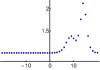
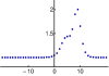
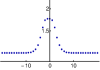
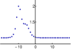
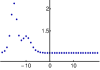
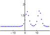
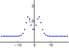
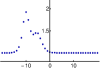
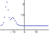
Figure 1: Plots of $V$ as a function of the discrete variable $j$, at times $-5,-3,0,3,5$, for the 2-soliton solution of the scalar version of the Volterra lattice system (2.67), elaborated in Example 2.6. Here we set $\lambda=1/2$, $\tilde{\lambda}=3/2$, and $-A_{1}=A_{2}=B_{1}=B_{2}=1$. The first row shows the solution without sources ($\tilde{\omega}=0$). The second row displays the solution with $\tilde{\omega}=10$.

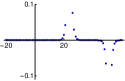
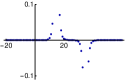
Figure 2: Plots of the source term $\hat{q}\,\tilde{r}_{(1)}$ as a function of the discrete variable $j$, at times $-15,-10,0,4$, for the 2-soliton solution of the scalar Volterra lattice equation with source, for which $V$ has been displayed in Fig. 1. The peaks vanish as $t\to\infty$ and separate into a positive and a negative bounded peak as $t\to-\infty$.

2.3.3 Exact solutions of the modified Volterra lattice equation with self-consistent sources

Here we have to choose $k=1$ and $l=-1$. Setting $P=\frac{1}{4}I-M^{2}$ and $Q=\frac{1}{4}I-\tilde{M}^{2}$, with arbitrary constant $n\times n$ matrices $M$ and $\tilde{M}$, (2.66) is satisfied by

$$\Lambda_{1,2}=-\frac{1}{2}I\pm M\,,\qquad\tilde{\Lambda}_{1,2}=-\frac{1}{2}I\pm\tilde{M}\,,$$

and we have

$$\theta=A_{1}\,e^{\Lambda_{1}^{-1}\,t}\,\Lambda_{1}^{j}+A_{2}\,e^{\Lambda_{2}^{-1}\,t}\,\Lambda_{2}^{j}\,,\qquad\eta=e^{-\tilde{\Lambda}_{1}^{-1}\,t}\,\tilde{\Lambda}_{1}^{-j}\,B_{1}+e^{-\tilde{\Lambda}_{2}^{-1}\,t}\,\tilde{\Lambda}_{2}^{-j}\,B_{2}\,,$$

with constant matrices $A_{a},B_{a}$, $a=1,2$, and

$$\tilde{\Omega} = e^{-\tilde{\Lambda}_{1}^{-1}\,t}\,\tilde{\Lambda}_{1}^{-j}\,X_{11}\,e^{\Lambda_{1}^{-1}\,t}\,\Lambda_{1}^{j}+e^{-\tilde{\Lambda}_{1}^{-1}\,t}\,\tilde{\Lambda}_{1}^{-j}\,X_{12}\,e^{\Lambda_{2}^{-1}\,t}\,\Lambda_{2}^{j}$$

$$+e^{-\tilde{\Lambda}_{2}^{-1}\,t}\,\tilde{\Lambda}_{2}^{-j}\,X_{21}\,e^{\Lambda_{1}^{-1}\,t}\,\Lambda_{1}^{j}+e^{-\tilde{\Lambda}_{2}^{-1}\,t}\,\tilde{\Lambda}_{2}^{-j}\,X_{22}\,e^{\Lambda_{2}^{-1}\,t}\,\Lambda_{2}^{j}+\tilde{\omega}\,,$$

where the constant matrices $X_{ab}$ have to solve the Stein equations

$$\tilde{\Lambda}_{1}\,X_{11}\,\Lambda_{1}^{-1}-X_{11}=B_{1}\,A_{1}\,,\qquad\tilde{\Lambda}_{1}\,X_{12}\,\Lambda_{2}^{-1}-X_{12}=B_{1}\,A_{2}\,,$$

$$\tilde{\Lambda}_{2}\,X_{21}\,\Lambda_{1}^{-1}-X_{21}=B_{2}\,A_{1}\,,\qquad\tilde{\Lambda}_{2}\,X_{22}\,\Lambda_{2}^{-1}-X_{22}=B_{2}\,A_{2}\,.$$

Then

$$g=(I-\theta\,\tilde{\Omega}_{(-1)}^{-1}\,\eta)\,g_{0}\,,\qquad\hat{q}=\theta\,\tilde{\Omega}_{(-1)}^{-1}\gamma_{i}\,,\qquad\tilde{r}=\tilde{\Omega}^{-1}\eta$$ (2.68)

solves (2.42) (with $k=1$ and $l=-1$) if $i=2$ and (2.49) if $i=1$, provided that $\tilde{\omega}$ satisfies the corresponding constraint. Via $U=V^{-1}=g_{(1)}\,g^{-1}$, this yields solutions of the two versions of the modified Volterra lattice equation with self-consistent sources. If $i=1$, in which case $\tilde{\omega}$ is constant, the latter reads (cf. (2.65))

$$U_{t}-U\,(U_{(1)}-U_{(-1)})\,U=U\,(\hat{q}\,\tilde{r}_{(1)})_{t}\,U\,,$$

$$\hat{q}_{t}=U_{(-1)}\,\hat{q}_{(-1)}\,,\qquad\tilde{r}_{t}=-\tilde{r}_{(1)}\,U\,.$$ (2.69)

Fig. 3 shows plots of a 2-soliton solution of the scalar version of this system ($m=n=1$). Fig. 4 displays the source term $\hat{q}\,\tilde{r}_{(1)}$.

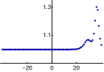
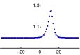
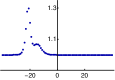
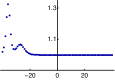
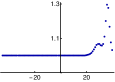
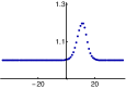
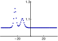
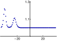
Figure 3: Plots of $U$ as a function of the discrete variable $j$, at times $-15,-5,8,14$, for the 2-soliton solution of the scalar modified Volterra lattice equation (2.69). The first row shows the source-free case ($\tilde{\omega}=0$), the second the corresponding solution with $\tilde{\omega}=-10$. Here we set $M=1/4$, $\tilde{M}=1/8$ and $-A_{1}=A_{2}=B_{1}=B_{2}=1$ in Section 2.3.3.

Figure 4: Plots of $\hat{q}\,\tilde{r}_{(1)}$ as a function of the discrete variable $j$, at times $-6,0,10,20,30$, for the 2-soliton solution of the scalar modified Volterra lattice equation with source, for which $U$ has been displayed in Fig. 3. The peaks vanish as $t\to-\infty$ and separate into spreading bounded peaks as $t$ becomes large.

3 On the second family of generalized Volterra lattice equations

The equation (2.14) in bidifferential calculus possesses a “Miura-dual” [22], which is

$$\mathrm{d}\bar{\mathrm{d}}\phi+\mathrm{d}\phi\,\mathrm{d}\phi=0\,$$ (3.70)

with $\phi\in\mathrm{Mat}(m,m,\mathcal{A})$. For this equation, there is the following counterpart of Theorem 2.2 [23].

Theorem 3.1.

Let $\phi_{0}$ be a solution of (3.70) and let $\theta$, $\eta$, $\Omega$ be solutions of the linear equations

$$\bar{\mathrm{d}}\theta=(\mathrm{d}\phi_{0})\,\theta+(\mathrm{d}\theta)\,\Delta+\theta\,\alpha\,,$$ (3.71)

$$\bar{\mathrm{d}}\eta=-\eta\,\mathrm{d}\phi_{0}+\Gamma\,\mathrm{d}\eta+\beta\,\eta\,,$$ (3.72)

$$\Gamma\,\Omega-\Omega\,\Delta=\eta\,\theta\,,$$ (3.73)

$$\bar{\mathrm{d}}\Omega=(\mathrm{d}\Omega)\,\Delta-(\mathrm{d}\Gamma)\,\Omega+\beta\,\Omega+\Omega\,\alpha+(\mathrm{d}\eta)\,\theta+\gamma\,,$$ (3.74)

where $\Delta,\Gamma,\alpha,\beta$ satisfy (2.17), $\gamma$ is given by (2.18) in terms of $\omega$, which has to satisfy (2.19). Then

$$\phi=\phi_{0}-\theta\,\Omega^{-1}\,\eta\,,\qquad q=\theta\,\Omega^{-1}\,,\qquad r=\Omega^{-1}\,\eta$$ (3.75)

constitutes a solution of

$$\mathrm{d}\,\bar{\mathrm{d}}\,\phi+\mathrm{d}\phi\;\mathrm{d}\phi=\mathrm{d}(q\,\gamma\,r)$$ (3.76)

and

$$\bar{\mathrm{d}}q=(\mathrm{d}\phi)\,q+\mathrm{d}(q\,\Gamma)-q\,\beta-q\,\gamma\,\Omega^{-1}\,,$$

$$\bar{\mathrm{d}}r=-r\,\mathrm{d}\phi+\mathrm{d}(\Delta\,r)-\alpha\,r-\Omega^{-1}\,\gamma\,r\,.$$ (3.77)

$\Box$

If a partial differential-difference equation can be realized via (3.70), by specifying the bidifferential calculus, then Theorem 3.1 allows to derive a corresponding binary Darboux transformation and also self-consistent source extensions (if $\gamma\neq 0$).

Remark 3.2.

Exploiting (3.70), using the bidifferential calculus determined by (2.13) and with $\phi=\varphi\,\mathbb{S}_{2}$, leads to

$$(\varphi_{,1}-\varphi)_{t}+(\varphi_{t}-I)(\varphi_{,2}-\varphi_{,1})-(\varphi_{,2}-\varphi_{,1})_{,-2}(\varphi_{t}-I)_{,1}=0\,.$$

Using (2.26), so that (2.27), (2.28) and (2.29) holds, one can derive corresponding self-consistent source extensions, a binary Darboux transformation and exact solutions. Via (2.16) the above equation leads to

$$(\tilde{\varphi}_{(k)}-\tilde{\varphi})_{t}+\tilde{\varphi}_{t}\,(\tilde{\varphi}_{(l)}-\tilde{\varphi}_{(k)})-(\tilde{\varphi}_{(l)}-\tilde{\varphi}_{(k)})_{(-l)}\,\tilde{\varphi}_{(k)t}=0\,,$$

where $\tilde{\varphi}=\varphi-t\,I$. But this equation is not (directly) related to any of the known families of generalized Volterra lattices.

In the following, we exploit Theorem 3.1 using the bidifferential calculus determined by (2.13), but with the roles of $\mathrm{d}$ and $\bar{\mathrm{d}}$ exchanged. Setting

$$\phi=\varphi\,\mathbb{S}_{2}^{-1}\,,$$

(3.70) then leads to

$$(\varphi_{,1}-\varphi)_{t}=(\varphi_{,2}-\varphi)(\varphi_{,1}-\varphi+I)-(\varphi_{,1}-\varphi+I)(\varphi_{,2}-\varphi)_{,1,-2}\,.$$ (3.78)

An equation equivalent to (3.78) appeared in [11] (see the theorem on page 41 therein). Applying the reduction (2.16), we obtain (1.11). Via (1.12) this results in the second family (1.10) of generalized Volterra lattice equations.

Remark 3.3.

According to Remark 2.1, we could also have addressed the first family of generalized Volterra lattice equations using (2.13) with the expressions for $\mathrm{d}$ and $\bar{\mathrm{d}}$ exchanged, thus treating both families using the same bidifferential calculus. Though this is indeed true, the elaboration of the first family would then have required a little more effort than what was needed in Section 2.

3.1 Self-consistent source extensions of (3.78)

We set

$$q=\tilde{q}\,\mathbb{S}_{2}^{-1}\,,\quad r=\mathbb{S}_{2}^{-1}\,\tilde{r}\,,\quad\Delta=\Gamma=\mathbb{S}_{2}^{-1}\,,$$

$$\alpha=(P+2I)\,\mathbb{S}_{1}\mathbb{S}_{2}^{-1}\,\xi_{1}+\xi_{2}\,,\quad\beta=-(Q+2I)\,\mathbb{S}_{1}\mathbb{S}_{2}^{-1}\,\xi_{1}-\xi_{2}\,,\quad$$

$$\Omega=-\mathbb{S}_{2}\,\tilde{\Omega}\,,\quad\omega=\tilde{\omega}\,\mathbb{S}_{2}\,,\quad\gamma=\gamma_{1}\,\mathbb{S}_{1}\,\xi_{1}+\gamma_{2}\,\mathbb{S}_{2}\,\xi_{2}\,.$$

Then $\tilde{q},\tilde{r},P,Q,\tilde{\omega}$ and $\tilde{\Omega}$ can be restricted to be matrices over $\mathcal{A}_{0}$ instead of $\mathcal{A}$ (with the algebras chosen in Section 2). (2.17) leads to (2.27), (2.19) to (2.28), and $\gamma_{1}$ and $\gamma_{2}$ are again given by the expressions (2.29). We will assume that $P$ and $Q$ are constant and that $\tilde{\omega}$ only depends on $t$.

(3.76) reads

$$(\varphi_{,1}-\varphi)_{t}+(\varphi_{,1}-\varphi+I)(\varphi_{,2}-\varphi)_{,1,-2}-(\varphi_{,2}-\varphi)(\varphi_{,1}-\varphi+I)\hskip 28.45274pt$$

$$\hskip 28.45274pt=(\tilde{q}_{,2}\,\gamma_{1}\,\tilde{r}_{,1,-2})_{,-2}-\tilde{q}_{,2}\,\gamma_{1}\,\tilde{r}_{,1,-2}+(\tilde{q}\,\gamma_{2}\,\tilde{r}_{,-2})_{,1}-\tilde{q}\,\gamma_{2}\,\tilde{r}_{,-2}\,.\qquad$$ (3.79)

(3.71) and (3.72) take the form

$$\tilde{q}_{,1,2} = -(\varphi_{,1}-\varphi+I)_{,2}\,\tilde{q}_{,1}-\tilde{q}_{,2}\,Q-\tilde{q}_{,2}\,\gamma_{1}\,\tilde{\Omega}_{,1}^{-1}\,,$$

$$\tilde{q}_{t} = \tilde{q}_{,2}+(\varphi_{,2}-\varphi)\,\tilde{q}+\tilde{q}\gamma_{2}\,\tilde{\Omega}^{-1}\,,$$

$$\tilde{r}_{,-2} = -\tilde{r}\,(\varphi_{,1}-\varphi+I)-P\,\tilde{r}_{,1,-2}+\tilde{\Omega}_{,2}^{-1}\,\gamma_{1}\,\tilde{r}_{,1,-2}\,,$$

$$\tilde{r}_{t} = -\tilde{r}_{,-2}-\tilde{r}\,(\varphi_{,2}-\varphi)+\tilde{\Omega}_{,2}^{-1}\,\gamma_{2}\,\tilde{r}\,.$$ (3.80)

We obtain the following self-consistent source extensions of (3.78).

1. $\gamma_{1}=0$, i.e., $Q\,\tilde{\omega}=\tilde{\omega}\,P$. In terms of $\hat{q}=\tilde{q}\,\gamma_{2}$ we obtain

   $$(\varphi_{,1}-\varphi)_{t}+(\varphi_{,1}-\varphi+I)(\varphi_{,2}-\varphi)_{,1,-2}-(\varphi_{,2}-\varphi)(\varphi_{,1}-\varphi+I)$$

   $$\hskip 21.33955pt=(\hat{q}\,\tilde{r}_{,-2})_{,1}-\hat{q}\,\tilde{r}_{,-2}\,,$$

   $$\hat{q}_{,1,2}=-(\varphi_{,1}-\varphi+I)_{,2}\,\hat{q}_{,1}-\hat{q}_{,2}\,P\,,$$

   $$\tilde{r}_{,-2}=-\tilde{r}\,(\varphi_{,1}-\varphi+I)-P\,\tilde{r}_{,1,-2}\,.$$

2. $\gamma_{2}=0$, i.e., $\tilde{\omega}_{t}=0$. We introduce $\hat{q}=\tilde{q}\,\gamma_{1}$.

   $$(\varphi_{,1}-\varphi)_{t}+(\varphi_{,1}-\varphi+I)(\varphi_{,2}-\varphi)_{,1,-2}-(\varphi_{,2}-\varphi)(\varphi_{,1}-\varphi+I)$$

   $$\hskip 62.59596pt=(\hat{q}_{,2}\,\tilde{r}_{,1,-2})_{,-2}-\hat{q}_{,2}\,\tilde{r}_{,1,-2}\,,$$

   $$\hat{q}_{t}=\hat{q}_{,2}+(\varphi_{,2}-\varphi)\,\hat{q}\,,\qquad\tilde{r}_{t}=-\tilde{r}_{,-2}-\tilde{r}\,(\varphi_{,2}-\varphi)\,.$$

3.2 Binary Darboux transformation

The linear equations (3.71), (3.72), (3.73) and (3.74) take the form

$$(\theta_{,1}+\theta\,P)_{,2}=-\theta_{,1}-(\varphi_{0,1}-\varphi_{0})_{,2}\,\theta_{,1}\,,\qquad\theta_{t}=\theta_{,2}+(\varphi_{0,2}-\varphi_{0})\,\theta\,,$$

$$(\eta+Q\,\eta_{,1})_{,-2}=-\eta-\eta\,(\varphi_{0,1}-\varphi_{0})\,,\hskip 35.56593pt\eta_{t}=-\eta_{,-2}-\eta\,(\varphi_{0,2}-\varphi_{0})\,,$$

$$\tilde{\Omega}_{,2}-\tilde{\Omega}=\eta\,\theta\,,\quad(\tilde{\Omega}\,P)_{,2}=Q\,\tilde{\Omega}_{,1}-\eta\,\theta_{,1}+\gamma_{1}\,,\quad\tilde{\Omega}_{t}=\eta_{,-2}\,\theta-\gamma_{2}\,.$$

For a given solution $\varphi_{0}$ of (3.78), we have to find solutions $\theta$ and $\eta$ of the first four equations. Then a corresponding solution of the equations for $\tilde{\Omega}$ has to be found. According to Theorem 3.1,

$$\varphi=\varphi_{0}+\theta\,\tilde{\Omega}^{-1}\,\eta_{,-2}\,,\qquad\tilde{q}=-\theta\,\tilde{\Omega}^{-1}\,,\qquad\tilde{r}=-\tilde{\Omega}_{,2}^{-1}\,\eta$$ (3.81)

then solve (3.79) and (3.80), and thus also the above self-consistent source systems, provided the respective condition for $\tilde{\omega}$ is fulfilled.

Remark 3.4.

For constant seed $\varphi_{0}$ and constant $P,Q$, the linear system for $\theta$ and $\eta$ coincides with that in (2.39). Therefore solutions are given by (2.40). Since in the case under consideration the above equations for $\tilde{\Omega}$ are equivalent to (2.37), $\tilde{\Omega}$ is given by (2.41). Now (3.81) provides us with an infinite set of solutions of (3.79) and (3.80).

3.3 Self-consistent source extensions of the second family of generalized Volterra lattices

Imposing the reduction (2.16), the systems obtained in Section 3.1 lead to

$$(\varphi_{(k)}-\varphi)_{t}+(\varphi_{(k)}-\varphi+I)(\varphi_{(l)}-\varphi)_{(k-l)}-(\varphi_{(l)}-\varphi)(\varphi_{(k)}-\varphi+I)$$

$$\hskip 22.76228pt=(\hat{q}\,\tilde{r}_{(-l)})_{(k)}-\hat{q}\,\tilde{r}_{(-l)}\,,$$

$$\;\hat{q}_{(k)}=-(\varphi_{(k)}-\varphi+I)\,\hat{q}_{(k-l)}-\hat{q}\,P\,,$$

$$\tilde{r}_{(-l)}=-\tilde{r}\,(\varphi_{(k)}-\varphi+I)-P\,\tilde{r}_{(k-l)}\,,$$ (3.82)

respectively

$$(\varphi_{(k)}-\varphi)_{t}+(\varphi_{(k)}-\varphi+I)(\varphi_{(l)}-\varphi)_{(k-l)}-(\varphi_{(l)}-\varphi)(\varphi_{(k)}-\varphi+I)$$

$$\hskip 65.44142pt=(\hat{q}_{(l)}\,\tilde{r}_{(k-l)})_{(-l)}-\hat{q}_{(l)}\,\tilde{r}_{(k-l)}\,,$$

$$\hat{q}_{t}=\hat{q}_{(l)}+(\varphi_{(l)}-\varphi)\,\hat{q}\,,\qquad\tilde{r}_{t}=-\tilde{r}_{(-l)}-\tilde{r}\,(\varphi_{(l)}-\varphi)\,.$$ (3.83)

Using (1.12), the corresponding self-consistent source extensions of (1.10) are

$$\Big{(}\sum_{i=0}^{k-1}W_{(i)}\Big{)}_{t}+\sum_{i=0}^{k-1}W_{(i)}\sum_{i=k-l}^{k-1}W_{(i)}-\sum_{i=0}^{l-1}W_{(i)}\sum_{i=0}^{k-1}W_{(i)}$$

$$\hskip 19.91684pt=(\hat{q}\,\tilde{r}_{(-l)})_{(k)}-\hat{q}\,\tilde{r}_{(-l)}\,,\hskip 227.62204pt$$

$$\hat{q}_{(k)}=-\sum_{i=0}^{k-1}W_{(i)}\,\hat{q}_{(k-l)}-\hat{q}\,P\,,\quad\tilde{r}_{(-l)}=-\tilde{r}\,\sum_{i=0}^{k-1}W_{(i)}-P\,\tilde{r}_{(k-l)}\,,$$ (3.84)

respectively

$$\Big{(}\sum_{i=0}^{k-1}W_{(i)}\Big{)}_{t}+\sum_{i=0}^{k-1}W_{(i)}\sum_{i=k-l}^{k-1}W_{(i)}-\sum_{i=0}^{l-1}W_{(i)}\sum_{i=0}^{k-1}W_{(i)}$$

$$\hskip 28.45274pt=(\hat{q}_{(l)}\,\tilde{r}_{(k-l)})_{(-l)}-\hat{q}_{(l)}\,\tilde{r}_{(k-l)}\,,$$

$$\hat{q}_{t}=\hat{q}_{(l)}+\Big{(}\sum_{i=0}^{l-1}W_{(i)}-\frac{l}{k}I\Big{)}\,\hat{q}\,,\quad\tilde{r}_{t}=-\tilde{r}_{(-l)}-\tilde{r}\,\Big{(}\sum_{i=0}^{l-1}W_{(i)}-\frac{l}{k}I\Big{)}\,.\hskip 34.14322pt$$ (3.85)

For $k=1$ and $l=2$, this yields further variants of a Volterra equation with sources:

$$W_{t}+W\,W_{(-1)}-W_{(1)}\,W=(\hat{q}\,\tilde{r}_{(-2)})_{(-1)}-\hat{q}\,\tilde{r}_{(-2)}\,,$$

$$\hat{q}_{(1)}=-W\,\hat{q}_{(-1)}-\hat{q}\,P\,,\qquad\tilde{r}_{(-2)}=-\tilde{r}\,W-P\,\tilde{r}_{(-1)})\,,$$

and

$$W_{t}+W\,W_{(-1)}-W_{(1)}\,W=(\hat{q}_{(2)}\,\tilde{r}_{(-1)})_{(-2)}-\hat{q}_{(2)}\,\tilde{r}_{(-1)}\,,$$

$$\hat{q}_{t}=\hat{q}_{(2)}+(W+W_{(1)}-2I)\,\hat{q}\,,\qquad\tilde{r}_{t}=-\tilde{r}_{(-2)}-\tilde{r}\,(W+W_{(1)}-2I)\,.$$

Remark 3.5.

With constant seed $\varphi_{0}$, we are led to exactly the same solutions for $\theta,\eta$ and $\tilde{\Omega}$ as in Section 2.3.1. Then

$$\varphi=\varphi_{0}+\theta\,\tilde{\Omega}^{-1}\,\eta_{(-l)}\,,\qquad\hat{q}=-\theta\,\tilde{\Omega}^{-1}\,\gamma_{i}\,,\qquad\tilde{r}=-\tilde{\Omega}_{(l)}^{-1}\,\eta$$ (3.86)

provides us with solutions of (3.82) if $i=2$, and of (3.83) if $i=1$. Via (1.12) this yields solutions of (3.84) and (3.85), respectively.

4 Conclusions

We have shown that the two families of generalized Volterra (or Bogoyavlensky) lattice equations arise from two semi-discrete integrable equations in three dimensions via reductions. All these equations possess a bidifferential calculus formulation that allows the application of general results concerning the construction of a binary Darboux transformation and self-consistent source extensions.

The systems extending generalized Volterra lattice equations to systems with sources, obtained in this work, fall into two types. The first type lacks evolution equations for the sources and, moreover, the equations constraining sources involve data of the solution-generating method, namely the $n\times n$ matrices $P$ or $Q$. This might look strange at first sight, but one has to keep in mind that, if the rank of $\omega$ is chosen smaller than $n$, only the corresponding part of those matrices enters the equations that govern the effective sources. The second type of systems contain evolution equations for all dependent variables. These systems are structurally analogous to systems obtained from higher-dimensional integrable systems (like KP) via a squared eigenfunction symmetry reduction. The method of [23] generates them without a detour to higher dimensions (which may not always be available).

It would have gone far beyond the scope of this work to analyze all the new systems and the generated families of solutions, which include multi-solitons. Only the Volterra and modified Volterra lattice equations with sources of the second type have been treated in more detail.

Acknowledgments. O.C. has been supported by an Alexander von Humboldt fellowship for postdoctoral researchers. We have to thank Aristophanes Dimakis for helpful discussions and several contributions to this work. We also would like to thank an anonymous referee for suggesting some useful additions to the original manuscript.

References

References

- [1] J. Moser, Finitely many mass points on the line under the influence of an exponential potential – an integrable system, in: Dynamical Systems, Theory and Applications, ed. J. Moser, Vol. 38 of Lecture Notes in Physics (Springer, 1975), 467–497.
- [2] M. Kac and P. van Moerbeke, On an explicitly soluble system of nonlinear differential equations related to certain Toda lattices, Adv. Math. 16 (1975) 160–169.
- [3] S.V. Manakov, Complete integrability and stochastization of discrete dynamical systems, Sov. Phys. JETP 40 (1975) 269–274.
- [4] M. Wadati, Transformation theories for nonlinear discrete systems, Progr. Theor. Phys. Suppl. 59 (1976) 36–63.
- [5] R. Hirota and J. Satsuma, -soliton solutions of nonlinear network equations describing a Volterra system, J. Phys. Soc. Jpn. 40 (1976) 891–900.
- [6] Y. Kajinaga and M. Wadati, A new derivation of the Bäcklund transformation for the Volterra lattice, J. Phys. Soc. Jpn. 67 (1998) 2237–2241.
- [7] K. Narita, Soliton solution to extended Volterra equation, J. Phys. Soc. Jpn. 51 (1982) 1682–1685.
- [8] O.I. Bogoyavlenskiĭ, Some constructions of integrable dynamical systems, Math. USSR Izvestiya 31 (1988) 47–75.
- [9] O.I. Bogoyavlenskiĭ, Integrable dynamical systems associated with the KdV equation, Math. USSR Izvestiya 31 (1988) 435–454.
- [10] O.I. Bogoyavlenskiĭ, The Lax representation with spectral parameter for certain dynamical systems, Math. USSR Izvestiya 32 (1989) 245–268.
- [11] O.I. Bogoyavlenskii, Algebraic constructions of integrable dynamical systems – extensions of the Volterra system, Russian Math. Surveys 46 (1991) 1–64.
- [12] X.-B. Hu and R.K. Bullough, Bäcklund transformation and nonlinear superposition formula of an extended Lotka-Volterra equation, J. Phys. A: Math. Gen. 30 (1997) 3635–3641.
- [13] X.-B. Hu and P.A. Clarkson, Rational solutions of an extended Lotka-Volterra equation, J. Nonl. Math. Phys. 9, Suppl. 1, (2002) 75–86.
- [14] K. Hikami and R. Inoue, The Hamiltonian structure of the Bogoyavlensky lattice, J. Phys. Soc. Japan 68 (1999) 776–783.
- [15] A. Dimakis and F. Müller-Hoissen, On generalized Lotka-Volterra lattices, Czech. J. Phys. 52 (2002) 1187–1193.
- [16] J.P. Wang, Recursion operator of the Narita-Itoh-Bogoyavlensky lattice, Stud. Appl. Math. 129 (2012) 309–329.
- [17] Y.B. Suris, The Problem of Integrable Discretization: Hamiltonian Approach, Vol. 219 of Progress in Mathematics (Birkhäuser, Basel, 2003).
- [18] A.K. Svinin, On some integrable lattice related by the Miura-type transformation to the Itoh-Narita-Bogoyavlenskii lattice, J. Phys. A: Math. Theor. 44 (2011) 465210.
- [19] G. Berkeley and S. Igonin, Miura-type transformations for lattice equations and Lie group actions associated with Darboux-Lax representations, arXiv:1512.09123v3.
- [20] V.E. Adler, Integrable Möbius invariant evolutionary lattices of second order, arXiv:1605.00018.
- [21] A. Dimakis and F. Müller-Hoissen, Bi-differential calculi and integrable models, J. Phys. A: Math. Gen. 33 (2000) 957–974.
- [22] A. Dimakis and F. Müller-Hoissen, Bidifferential graded algebras and integrable systems, Discr. Cont. Dyn. Systems Suppl. 2009 (2009) 208–219.
- [23] O. Chvartatskyi, A. Dimakis and F. Müller-Hoissen, Self-consistent sources for integrable equations via deformations of binary Darboux transformations, Lett. Math. Phys. 106 (2016) 1139–1179.
- [24] F. Yu, A non-isospectral integrable couplings of Volterra lattice hierarchy with self-consistent sources, Appl. Math. Comp. 215 (2009) 1217–1223.
- [25] Y. Itoh, Integrals of a Lotka-Volterra system of odd number of variables, Prog. Theor. Phys. 78 (1987) 507–510.
- [26] Y.B. Suris, Integrable discretizations for lattice system: local equations of motion and their Hamiltonian properties, Rev. Math. Phys. 11 (1999) 727–822.
- [27] B. Qin, B. Tian, L.-C. Liu, M. Wang, Z.-Q. Lin and W.-J. Liu, Bell-polynomial approach and -soliton solution for the extended Lotka-Volterra equation in plasmas, J. Math. Phys. 52 (2011) 043523.
- [28] A. Dimakis and F. Müller-Hoissen, Binary Darboux transformations in bidifferential calculus and integrable reductions of vacuum Einstein equations, SIGMA 9 (2013) 009.