Electric potential and field calculation of charged BEM triangles and rectangles by Gaussian cubature

Abstract

It is a widely held view that analytical integration is more accurate than the numerical one. In some special cases, however, numerical integration can be more advantageous than analytical integration. In our paper we show this benefit for the case of electric potential and field computation of charged triangles and rectangles applied in the boundary element method (BEM). Analytical potential and field formulas are rather complicated (even in the simplest case of constant charge densities), they have usually large computation times, and at field points far from the elements they suffer from large rounding errors. On the other hand, Gaussian cubature, which is an efficient numerical integration method, yields simple and fast potential and field formulas that are very accurate far from the elements. The simplicity of the method is demonstrated by the physical picture: the triangles and rectangles with their continuous charge distributions are replaced by discrete point charges, whose simple potential and field formulas explain the higher accuracy and speed of this method. We implemented the Gaussian cubature method for the purpose of BEM computations both with CPU and GPU, and we compare its performance with two different analytical integration methods. The ten different Gaussian cubature formulas presented in our paper can be used for arbitrary high-precision and fast integrations over triangles and rectangles.

1 Introduction

Triangles and rectangles have many applications in mathematics, engineering and science. The finite element method [1, 2, 3, 4] (FEM) and the boundary element method [4, 5, 6, 7, 8, 9, 10] (BEM) rely especially heavily on triangles and rectangles as basic elements for their discretization procedure. In order to obtain the system of equations with the nodal function values of the elements in FEM and BEM, numerical or analytical integrations over the elements are needed.

The main subject of our paper is 3-dimensional electric potential and field calculation of charged triangular and rectangular BEM elements. Electric field calculation is important in many areas of physics: electron and ion optics, charged particle beams, charged particle traps, electron microscopy, electron spectroscopy, plasma and ion sources, electron guns, etc. [11, 12]. A special kind of electron and ion energy spectroscopy is realized by the MAC-E filter spectrometers, where the integral energy spectrum is measured by the combination of electrostatic retardation and magnetic adiabatic collimation. Examples are the Mainz and Troitsk electron spectrometers [13, 14], the aSPECT proton spectrometer [15], and the KATRIN pre- and main electron spectrometers [16, 17, 18]. High accuracy electric field and potential computations are indispensable for precise and reliable charged particle tracking calculations for these experiments. For this purpose the open source C++ codes KEMField [19] and Kassiopeia [20, 22, 21] are used in the KATRIN and aSPECT experiments.

For the purpose of electric potential and field computation with BEM [11, 12, 23, 10], the surface of the electrodes is discretized by many small boundary elements, and a linear algebraic equation system is obtained for the unknown charge densities of the individual elements. To solve these equations, either a direct or an iterative method is used. When the charge densities are known, the potential and field at an arbitrary point (called field point) can be computed by summing the potential and field contributions of all elements. The electric potential and field of a single charged element at the field point can be expressed by analytical or numerical integration of the point-charge Coulomb formula times the charge density over the element surface. In the simplest case of constant BEM element, the charge density is assumed to be constant over the element surface.

It is a general belief that analytical integration is more accurate than numerical integration. This is in many cases true, but not always. A simple example with one-dimensional integral and small integration interval (Sec. 2) shows that analytical integration can have a large rounding error, due to the finite arithmetic precision of the computer [24, 25], while a simple numerical integration has in this case a much higher accuracy. Analytically calculated electric potential and field formulas of charged triangles and rectangles show a similar behavior for large distance ratios; the latter is defined as the distance of the element center and the field point divided by the average side length of the element: for field points far from the element the distance ratio is large. Sec. 2 presents a few plots for the relative error of the analytical potential and field of triangles and rectangles as a function of the distance ratio. One can see that for field points far from the element the analytically computed potential and field values have significant rounding errors that are much higher than the machine epsilon of the corresponding arithmetic precision [24, 25] that is used for the computation. The analytical integration formulas of Refs. [19, 26] and [27, 28] were used for these plots. There are many other published analytical integration results for potential and field calculation of triangles and rectangles [29, 30, 31, 32, 33, 34, 35, 36, 38, 37], and these suffer probably from the same rounding error that increases with the distance ratio. The rounding errors are caused by the transcendental functions (e.g. log, atan2 etc.) in the analytical formulas and by the well-known subtraction cancellation problem of finite-digit floating-point arithmetic computations. Another disadvantage of the analytical integrations is that the analytical potential and field formulas are rather complicated, and consequently the calculations are rather time consuming.

According to the aforementioned simple example with one-dimensional integration, one can eliminate the rounding error problem of the analytical potential and field calculations by using numerical integration. The two-dimensional numerical integration could be performed by two subsequent one-dimensional integrations, using e.g. the efficient Gauss-Legendre quadrature method with 16 nodes for each dimension [39, 40]. If the field point is not too close to the triangle or rectangle, this bi-quadrature method results in very accurate integral values. In fact, we use this method as a reference integration in order to define the errors of the other integration methods. Nevertheless, if the goal is also to minimize the computation time, then it is more expedient to use the Gaussian cubature method for two-dimensional numerical integration, because it has fewer function evaluations for a targeted accuracy. In Sec. 3 we present a short overview about the numerical integration of an arbitrary function over a triangle or a rectangle with Gaussian cubature. The integral is approximated by a weighted sum of the function values at a given number of Gaussian points. The accuracy of this approximation is defined by the degree of the cubature formula, which usually increases with the number $N$ of Gaussian points. Appendices A and B contain ten tables of the Gaussian points and weights of five different Gaussian cubature formulas for triangles and rectangles. These formulas have various number of Gaussian points (from $N=4$ to $N=33$) and degrees of accuracy (from 3 to 13).

In Sec. 4 we apply the general Gaussian cubature formulas for electric potential and field calculation of triangles and rectangles with constant charge density. The mathematical formalism of the Gaussian cubature integration is illustrated by a nice physical picture: the triangles and rectangles with continuous charge distribution are replaced by discrete point charges, and the complicated two-dimensional integration of the potential-field calculation is substantially simplified by using the potential and field formulas of point charges. The figures in Sec. 4 reveal that for field points far from the elements the Gaussian cubature method has high accuracy and is exempt from the rounding error problem of the analytical integrations. The relative error of the potential and field calculation with a given Gaussian cubature formula is about $10^{-15}$ above some distance ratio limit (with double precision computer arithmetics), and increases with decreasing distance ratio below this limit, which decreases with increasing number of Gaussian points (i.e. for more accurate cubature formulas). For small distance ratios, e.g. ${\rm DR}<3$, the Gaussian cubature formulas presented in our paper are not accurate enough, and analytical integration should be used in this region.

Sec. 5 contains results for accuracy comparisons of potential and field simulations with two complex electrode geometries containing 1.5 million triangles and 1.5 million rectangles, respectively. The table in this section shows that the relative errors of the Gaussian cubature calculations are much smaller than the errors of the analytical calculations. In fact, the Gaussian cubature relative error values are close to $10^{-15}$, i.e. the best accuracy that is possible to obtain with the double precision arithmetic that is used in these computations. Sec. 6 presents an additional advantage of the Gaussian cubature method: the potential and field calculations with low-$N$ cubature formulas are significantly faster than the corresponding simulations with analytical integration. E.g. the 7-point cubature method in CPU computations is about five times faster than the analytical integration method of Ref. [27, 28] and more than ten times faster than the analytical integration method of Ref. [19]. The larger speed of the Gaussian cubature method is due to its simplicity: it needs the evaluation of only one square root and one division operation for each Gaussian point, in addition to multiplications and additions, while the analytical integration methods need many time consuming transcendental function evaluations (like log, atan2 etc.). Of course, for the elements with smaller distance ratios the cubature formulas with larger number of points (e.g. 12, 19 or 33) have to be used (to get an acceptable accuracy level), and they are slower (although still faster than the analytical methods). Nevertheless, the distance ratio distribution plots in Sec. 5 show that for most of the elements of a typical electrode geometry the fast 7-point cubature method can be used.

2 Analytical integration

Let us first consider the simple one-dimensional integral of the function $\exp(x)$ from 1 to $1+\delta$. The analytical result from the Newton-Leibniz formula is $\exp(1+\delta)-\exp(1)$, and this is for small $\delta$ a typical example for loss of accuracy (digits) when subtracting two almost equal numbers. The problem is that the computer stores in a floating-point arithmetic number always a finite number of digits [24, 25], and a few of them can disappear at subtraction. Therefore, the relative error of the above integral for small $\delta$ is much larger than the machine epsilon of the floating-point number system that is used for the computation.

If a high accuracy is required for the integral value with small $\delta$, it is better to use numerical integration, e.g. Gaussian quadrature. With double precision arithmetic and with Gauss-Legendre quadrature [39, 40] using 16 x 16 integration nodes, the relative error of the integral is smaller than $10^{-15}$, i.e. the numerical integration has the maximal precision that is possible to achieve with the corresponding floating-point number system. One can see this by the independence of the integral value on the number of integration nodes, or by comparing with a higher precision (e.g. long double) computation. Due to this fact, we can get the accuracy of the analytical integral values by comparing them with the numerical quadrature values: ${\rm err}(I_{an})=|(I_{an}-I_{num})/I_{num}|$.

Fig. 1 presents the relative error ${\rm err}(I_{an})$ of the analytical integral above as a function of $1/\delta$, for three different C++ floating-point arithmetic types: float, double and long double. The relative error increases with $1/\delta$ and decreases with increasing precision of the floating-point arithmetic. It is then obvious that the analytical integration has a rounding error which can be for small integration interval size $\delta$ much larger than the precision of the floating-point arithmetic type that is used for the calculation. The numerical integration (like Gaussian quadrature) is, however, devoid of this precision loss problem.

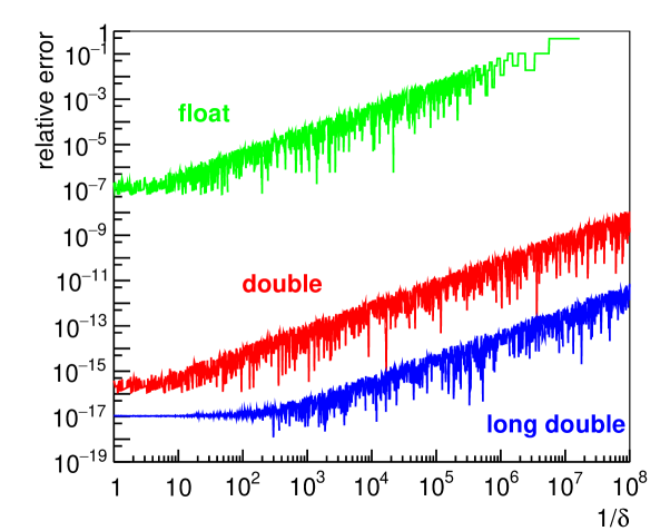
Figure 1: Relative error of the one-dimensional analytical integral $\exp(1+\delta)-\exp(1)$ as function of $1/\delta$, for float, double and long double C++ arithmetic types.

Let us continue now with electric potential and field computation of triangles and rectangles with constant charge density $\sigma$. The potential $\Phi$ and field ${\bf E}$ at field point ${\bf P}$ can be generally written (in SI units) as surface integrals over the element:

$$\Phi({\bf P})=\frac{\sigma}{4\pi\varepsilon_{0}}\int\limits_{\rm element}d^{2}{\bf Q}\cdot\frac{1}{|{\bf P}-{\bf Q}|},\quad\quad{\bf E}({\bf P})=\frac{\sigma}{4\pi\varepsilon_{0}}\int\limits_{\rm element}d^{2}{\bf Q}\cdot\frac{{\bf P}-{\bf Q}}{|{\bf P}-{\bf Q}|^{3}},$$ (2.1)

where ${\bf Q}$ denotes the integration point on the element surface. We introduce the distance $D$ between the field point ${\bf P}$ and the center point (centroid) ${\bf Q_{\rm cen}}$ of the triangle or rectangle: $D=|{\bf P}-{\bf Q_{\rm cen}}|$, and the average side length $L$ of the triangle or rectangle (e.g. $L=(a+b+c)/3$, with triangle side lengths $a$, $b$ and $c$). Then, the distance ratio of the element and field point combination is defined as ${\rm DR}=D/L$; this corresponds to the $1/\delta$ parameter of the one-dimensional integral described above.

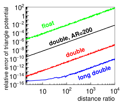
(a) TrianglePotential

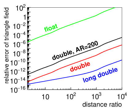
(b) TriangleField

Figure 2: Averaged relative error of the analytically computed triangle potential (Refs. [19, 26], left) and triangle field (Refs. [27, 28], right), as a function of the distance ratio, for float (green), double (red) and long double (blue) C++ arithmetic types (with low aspect ratio triangles), and with double precision and high aspect ratio (AR=200) triangles (black).

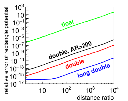
(a) RectanglePotential

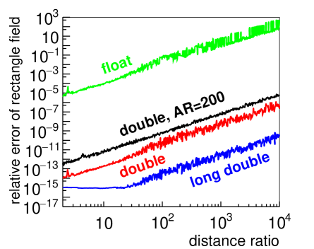
(b) RectangleField

Figure 3: Averaged relative error of the analytically computed rectangle potential (Refs. [27, 28], left) and rectangle field (Ref. [19], right), as a function of the distance ratio, for float (green), double (red) and long double (blue) C++ arithmetic types (with low aspect ratio rectangles), and with double precision and high aspect ratio (AR=200) rectangles (black).

In order to investigate the potential and field calculation of triangles and rectangles, we carried out the following procedure. First, we generated the corner points of triangles or rectangles randomly inside a cube with unit lengths and the direction unit vector of the field point also randomly relative to the triangle or rectangle centroid. Then, for a fixed distance ratio both the element (triangle or rectangle) and the field point are defined. We computed the potential and field of the element with unit charge density at the field point by two different analytical integration methods: first, with Refs. [19] (App. A and B) and [26] (App. A), and second, with Refs. [27] (Eqs. 63 and 74) and [28]. In order to obtain the error of the analytical integrals, we also calculated the potential and field by numerical integration, using two successive one-dimensional Gauss-Legendre quadratures (GL2) [39, 40] with $n_{GL2}=16$ integration nodes for both integrations. If the field point is located not too close to the element (i.e. for distance ratio above two), the latter method yields a relative accuracy which is close to the precision of the applied floating-point arithmetic type (e.g. order of $10^{-15}$ for double precision in C++). One can check that the GL2 integral values do not change if the discretization number $n_{GL2}$ is changed, and possible rounding errors can be tested by comparing double and long double calculations. The relative error of the analytically computed potential is then: ${\rm err}(\Phi_{an})=|(\Phi_{an}-\Phi_{GL2})/\Phi_{GL2}|$. For the field ${\bf E}$ we define the relative error in the following way: ${\rm err}({\bf E}_{an})=\sum_{j=x,y,z}|{\bf E}_{j,an}-{\bf E}_{j,GL2}|/|{\bf E}|_{GL2}$, where the sum goes over the components $x$, $y$ and $z$. We generate 1000 elements and field point direction vectors for each distance ratio, and we take the average of the above defined relative error values. In this case the triangles and rectangles have small (mainly below ten) aspect ratios (AR). The triangle aspect ratio is defined as the longest side length divided by the corresponding height. Similarly, the rectangle aspect ratio is the longer side divided by the shorter side.

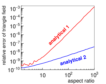
(a) Triangles

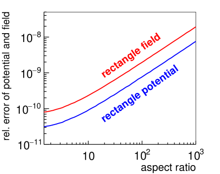
(b) Rectangles

Figure 4: Averaged relative error of the analytically computed triangle field (left, 1 (red): Ref. [19], 2 (blue): Ref. [27]), and rectangle potential and field (right, Ref. [27]; Ref. [19] is similar), as a function of the aspect ratio, with fixed distance ratio DR=300.

Figures 2 and 3 present the above defined averaged relative errors for triangle and rectangle potential and field, computed by the analytical integration formulas of Refs. [19, 26, 27, 28], as a function of the distance ratio, for three different floating-point arithmetic types (float, double and long double of the C++ language) with low aspect ratio elements, and also for larger (AR=200) aspect ratio elements. For small distance ratio (below five), the relative error values are close to the corresponding floating-point arithmetic precision. Note that our Gauss-Legendre quadrature implementation has double precision accuracy, therefore the relative error in case of long double precision is not smaller than $10^{-15}$ or so. Furthermore, the plots show that the relative error of the analytical integrals increases with the distance ratio and also with the aspect ratio, while it decreases with increasing precision of the floating-point arithmetic type.

It is obvious that the analytical integrals have significant rounding errors for large distance ratio. These potential and field errors are even much larger for triangles and rectangles with large aspect ratio, as one can see in Fig. 4. We conjecture that all other analytically integrated potential and field formulas in the literature (Refs. [29, 30, 31, 32, 33, 34, 35, 36, 38, 37]) have similarly large rounding errors for field points located far from the elements.

3 Numerical integration with Gaussian cubature

The rounding error problem of the analytical integration can be solved by using numerical integration for field points far away from the element. Gaussian quadrature and cubature are efficient numerical integration techniques [39, 40, 41, 42, 43] which can yield high accuracies with a minimal number of nodes (function evaluation points).

The integral of an arbitrary function $f$ over a surface element can be generally approximated by Gaussian cubature as

$$\int\limits_{\rm element}d^{2}{\bf Q}\cdot f({\bf Q})={\cal A}\cdot\sum_{i=1}^{N}w_{i}\cdot f({\bf Q}_{i})+{\cal R},\quad\quad\sum_{i=1}^{N}w_{i}=1,$$ (3.1)

where ${\bf Q}_{i}$ and $w_{i}$ are the Gaussian points (nodes, knots) and weights, respectively, and ${\cal A}$ denotes the area of the element. The remainder ${\cal R}$ is the absolute error of the Gaussian cubature integral formula.

To parametrize the Gaussian points ${\bf Q}_{i}$, it is expedient to use local coordinates: they rely on the element geometry for their definition and are generally called natural coordinates [1, 3, 2]. In the case of rectangles, it is advantageous to use a local coordinate system whose axes are parallel with the side unit vectors ${\bf u}_{x}$ and ${\bf u}_{y}$ of the rectangle. An arbitrary point ${\bf Q}$ on the plane of the rectangle can be parametrized by the local natural coordinates $x$ and $y$:

$${\bf Q}={\bf Q}_{\rm cen}+\frac{a}{2}\,x\,{\bf u}_{x}+\frac{b}{2}\,y\,{\bf u}_{y},$$ (3.2)

where ${\bf Q}_{\rm cen}$ denotes the rectangle center, and $a$ and $b$ are the two side lengths; see Fig. 5(a). For $|x|\leq 1$ and $|y|\leq 1$ the point ${\bf Q}$ is inside the rectangle, otherwise it is outside.

For the parametrization of points in a triangle it is advantageous to use the so-called barycentric or area coordinates. An arbitrary point ${\bf Q}$ on the plane of the triangle can be written as a linear combination of the triangle vertex vectors ${\bf A}$, ${\bf B}$ and ${\bf C}$:

$${\bf Q}=\lambda_{A}{\bf A}+\lambda_{B}{\bf B}+\lambda_{C}{\bf C},\quad{\rm with}\quad\lambda_{A}+\lambda_{B}+\lambda_{C}=1,$$ (3.3)

where $\lambda_{A}$, $\lambda_{B}$ and $\lambda_{C}$ are the barycentric coordinates. They are all less than 1 if the point ${\bf Q}$ is inside the triangle. For $\lambda_{A}=1,\;\lambda_{B}=\lambda_{C}=0$: ${\bf Q}={\bf A}$, and for $\lambda_{A}=0$ the point ${\bf Q}$ is on the line ${\bf BC}$. $\lambda_{A}=\lambda_{B}=\lambda_{C}=1/3$ corresponds to the centroid of the triangle. The coordinate $\lambda_{A}$ is equal to the ratio of the triangle areas ${\bf QBC}$ and ${\bf ABC}$ (and similarly for $\lambda_{B}$ and $\lambda_{C}$), as one can see in Fig. 5(b). Due to this property, the barycentric coordinates are also called area coordinates (see Refs. [1, 2, 3]).

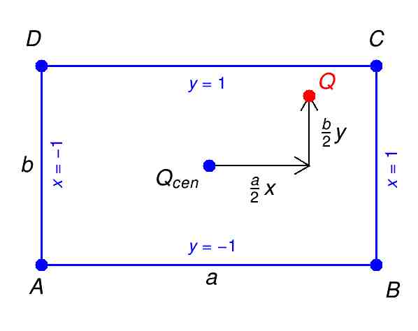
(a) Rectangle

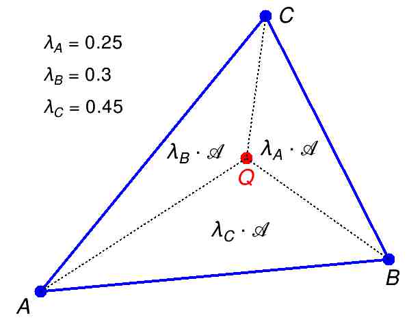
(b) Triangle

Figure 5: Natural local coordinates on a rectangle (left) and barycentric (area) coordinates on a triangle (right).

The computation time of a Gaussian cubature formula is proportional to the number of Gaussian points (nodes) $N$. A good formula has small error (remainder ${\cal R}$ in Eq. 3.1) with small $N$. Usually, a two-dimensional Gaussian cubature formula is constructed so that it is exact (with ${\cal R}=0$) for all possible monomials $f(x,y)=x^{n}y^{m}$ with $0\leq n+m\leq d$, but for $n+m>d$ the remainder ${\cal R}$ is not zero. The integer $d$ is called the degree of the cubature formula. A large degree $d$ corresponds to high accuracy, but the number of nodes $N$, and so the computation time, also increases with $d$.

The definition of the degree above makes it plausible how to determine the nodes and weights for two-dimensional Gaussian cubature formulas: first, one calculates the integral (analytically or numerically) on the left-hand side of Eq. 3.1 for several different monomial functions $f(x,y)=x^{n}y^{m}$ (with $n+m\leq d$). Then, each integral value is set equal to the cubature sum formula on the right-hand side of Eq. 3.1 (with ${\cal R}=0$). One obtains then the nodes and weights by solving this nonlinear equation system, which is obviously a difficult task, especially for large $N$ and $d$. It is expedient to have all weights positive (to reduce rounding errors) and all nodes inside the element.

Gaussian point coordinates and weights for triangles and rectangles with various $N$ and $d$ values can be found in several books [41, 42, 43] and in many publications [44, 45, 46, 47, 48, 49, 50, 51, 52, 53, 54, 55, 56, 57, 58, 59, 60, 61, 62]. Examples for very high degree cubature formulas are: $N=175,\,d=30$ for triangles in [61], and $N=100,\,d=23$ for rectangles in [56]. There are several review papers about the subject in the literature [63, 64, 65, 66, 67, 68].

In App. A we present barycentric coordinates and weights of five different Gaussian cubature formulas for triangles: $N=4,\,d=3$ (Table A1), $N=7,\,d=5$ (Table A2), $N=12,\,d=7$ (Table A3), $N=19,\,d=9$ (Table A4) and $N=33,\,d=12$ (Table A5). App. B contains cartesian natural coordinates and weights of five different Gaussian cubature formulas for rectangles: $N=4,\,d=3$ (Table B1), $N=7,\,d=5$ (Table B2), $N=12,\,d=7$ (Table B3), $N=17,\,d=9$ (Table B4) and $N=33,\,d=13$ (Table B5). In most cases, one row in a table corresponds to several nodes with equal weights: the coordinates of the other nodes can be obtained by various permutations or sign changes of the given numbers (see the table captions for detailed explanations).

Figures 6 and 7 show a few examples for the Gaussian points of a triangle and a rectangle. In Fig. 6(a), point 1 corresponds to the first row in Table A2 (this is the centroid of the triangle). Points 2 to 4 correspond to the second row: for point 2 $\to\lambda_{A}=t+2ts$, for point 3 $\to\lambda_{B}=t+2ts$, and for point 4 $\to\lambda_{C}=t+2ts$ (the other barycentric coordinates are $t-ts$). Similarly, points 5 to 7 correspond to the third row in that table. These figures can be useful to understand the multiplicity structure of the tables in App. A and B.

(a) Triangle7

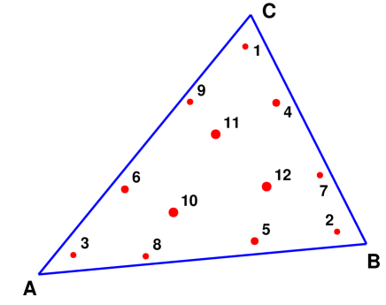
(b) Triangle12

Figure 6: Gaussian points of the 7-point (left) and the 12-point (right) cubature formula for triangle. The numbers are the indices of the Gaussian points. The surfaces of the red circles are proportional to the corresponding weights.

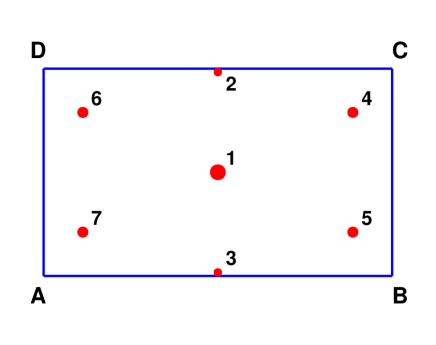
(a) Rectangle7

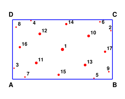
(b) Rectangle17

Figure 7: Gaussian points of the 7-point (left) and the 17-point (right) cubature formula for rectangle. The numbers are the indices of the Gaussian points. The surfaces of the red circles are proportional to the corresponding weights.

4 Potential and field calculation by Gaussian cubature

The electric potential and field of an arbitrary constant BEM element (with constant charge density $\sigma$) at a field point ${\bf P}$ can be approximated by Gaussian cubature as:

$$\Phi({\bf P})\approx\frac{1}{4\pi\varepsilon_{0}}\sum_{i=1}^{N}\frac{q_{i}}{|{\bf P}-{\bf Q}_{i}|},\quad\quad{\bf E}({\bf P})\approx\frac{1}{4\pi\varepsilon_{0}}\sum_{i=1}^{N}q_{i}\frac{{\bf P}-{\bf Q}_{i}}{|{\bf P}-{\bf Q}_{i}|^{3}},$$ (4.1)

where $q_{i}=w_{i}q$ denotes the charge of point $i$, and $q=\sigma{\cal A}$ is the total charge of the element. We have then a nice and intuitive physical picture of the Gaussian cubature formalism: the BEM element with continuous charge density is replaced by discrete point charges, whereas the charge $q_{i}$ at the Gaussian point ${\bf Q}_{i}$ is proportional to the Gaussian weight $w_{i}$, and the sum of the individual charges $q_{i}$ is equal to the total charge of the element (see Eq. 3.1). Obviously, it is much more easier to compute the potential and field produced by point charges instead of continuous charge distributions. As we will see below, the point charge method is not only easier but also more precise, at least for field points which are not too close to the element. In addition, the point charge calculation is typically faster than the analytical integration with continuous charge distribution (see Sec. 6).

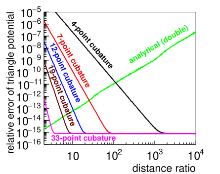
(a) TrianglePotential

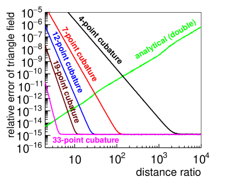
(b) TriangleField

Figure 8: Averaged relative error of the triangle potential (left) and field (right) for the 5 Gaussian cubature approximations of App. A, as a function of the distance ratio. For comparison, the averaged relative error of the triangle potential and field computed by analytical integration (Refs. [27, 28]) is also shown.

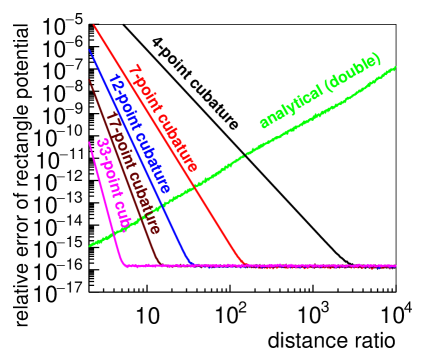
(a) RectanglePotential

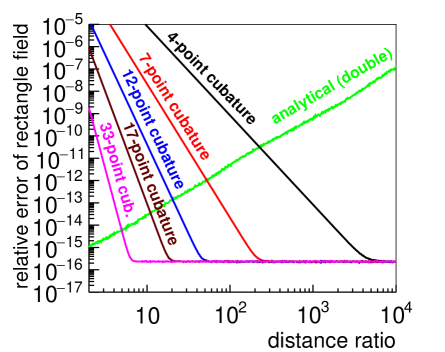
(b) RectangleField

Figure 9: Averaged relative error of the rectangle potential (left) and field (right) for the 5 Gaussian cubature approximations of App. B, as a function of the distance ratio. For comparison, the averaged relative error of the rectangle potential and field computed by analytical integration (Refs. [27, 28]) is also shown.

In order to investigate the performance of the Gaussian cubature or point charge approximation for potential and field calculation of triangles and rectangles, we used the same procedure that is described in Sec. 2. First, for a fixed element and field point, the relative error of the potential computed by Gaussian cubature is defined as: ${\rm err}(\Phi_{cub})=|(\Phi_{cub}-\Phi_{GL2})/\Phi_{GL2}|$, where $\Phi_{GL2}$ is computed by two-dimensional Gauss-Legendre integration. A similar formula holds for the field error (see in Sec. 2). Then, 1000 elements and field point directions are randomly generated for a fixed distance ratio, and the averages of the relative error values are calculated for 500 different distance ratio values from 2 to 10000.

Figures 8 and 9 present the averaged relative error of the potential and field for triangles and rectangles as a function of the distance ratio, for the ten Gaussian cubature approximations described in App. A and B, together with the relative error of the analytical integration described in Refs. [27, 28] (with double precision arithmetic type). One can see that, while the relative error of the analytical integration is small for field points close to the element (small distance ratio), and it increases with the distance ratio, the behavior of the Gaussian cubature error is just the opposite: it is large for field points near the element, and it decreases with the distance ratio. In fact, the accuracy of the Gaussian cubature at high distance ratio is limited only by the finite-digit computer arithmetic precision. Therefore, it seems that the analytical and numerical integration methods complement each other: to get high accuracy everywhere, one should use analytical integration for field points close to the element and numerical integration farther away.

It is also conspicuous from the figures that the cubature formulas with more Gaussian points $N$ have higher accuracy and can be used also for field points closer to the elements to obtain a given accuracy level (e.g. $10^{-15}$). The computation time for the potential or field simulation by Gaussian cubature is approximately proportional to $N$, therefore, in order to minimize the computation time, it is expedient to use several different cubature formulas: for large distance ratio DR one can use a cubature formula with smaller $N$, and for smaller DR one should use a formula with larger $N$. E.g. to obtain $2\cdot 10^{-15}$ relative accuracy level for the triangle potential, one should use the following cubature formulas in the various distance ratio intervals: $N=4$ for ${\rm DR}>1500$, $N=7$ for $80<{\rm DR}<1500$, $N=12$ for $20<{\rm DR}<80$, $N=19$ for $8<{\rm DR}<20$, $N=33$ for $3<{\rm DR}<8$, and analytical integration for ${\rm DR}<3$. In the case of triangle field these limits are slightly higher. If both the potential and the field has to be computed for a field point in one computation step, then one should use the limits defined by the field; namely, in this case the same Gaussian points and weights can always be used for both calculations.

We showed in Sec. 2 that the relative error of the analytically computed potential and field increases with the triangle and rectangle aspect ratio. We investigated the aspect ratio dependence also for Gaussian cubature. Fig. 10 presents the error of the 7-point Gaussian cubature field as a function of the aspect ratio, for DR=300 distance ratio; the potential error and higher-order Gaussian cubatures have a similar behavior. One can see that the triangle potential and field error of the Gaussian cubature increases with the aspect ratio. Therefore, a large number of triangles with high aspect ratios should be avoided in BEM calculations, if high accuracy computations are required. On the other hand, the Gaussian cubature potential and field calculations of rectangles seem not to be sensitive to the rectangle aspect ratio.

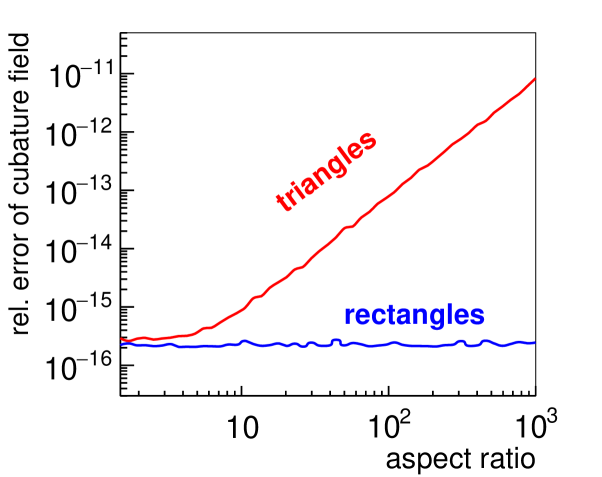
Figure 10: Averaged relative error of the 7-point Gaussian cubature field for triangles and rectangles as a function of the aspect ratio, for a fixed distance ratio DR=300.

Finally, we mention that a triangle can be mapped into a rectangle by the Duffy transformation [69, 64], therefore the numerical integration over a triangle by Gaussian cubature can also be done by using the Duffy transformation in conjunction with the Gaussian cubature formulas for rectangles of App. B, instead of the triangle formulas of App. A. In this case, however, we get much larger errors for the potential and field of triangles than by using the Gaussian cubature formulas for triangles. E.g. the relative error of the triangle field at DR=100 with the Duffy transformation and the 7-point rectangle cubature formula is about $10^{-8}$, in contrast with the few times $10^{-15}$ error of the triangle 7-point Gaussian cubature formula (see Fig. 8(b)).

5 Accuracy comparisons with complex geometries

The main goal of potential and field calculation of charged triangles and rectangles is to apply these elements for electric potential and field computations of complex electrode systems with BEM. Therefore, it is important to compare the accuracy of the analytical and numerical integration methods not only for individual elements, but also for electrode systems with many elements. In this section, we present results for two electric field simulations: one of them contains only triangles as BEM elements, the other one only rectangles. For this purpose, we discretized the main spectrometer vessel and inner electrodes of the KATRIN experiment first by 1.5 million triangles and second by 1.5 million rectangles, using a dipole electrode potential configuration. The KATRIN main spectrometer inner electrode system has a complicated wire electrode system [70] but in our models the wire electrodes are replaced by full electrode surfaces. Fig. 11 shows a two-dimensional plot (z-y plane) of the KATRIN main spectrometer vessel and inner electrode system. For further details about this spectrometer we refer to Ref. [18]. The dipole electrode model discretizations are explained in detail in Ref. [77].

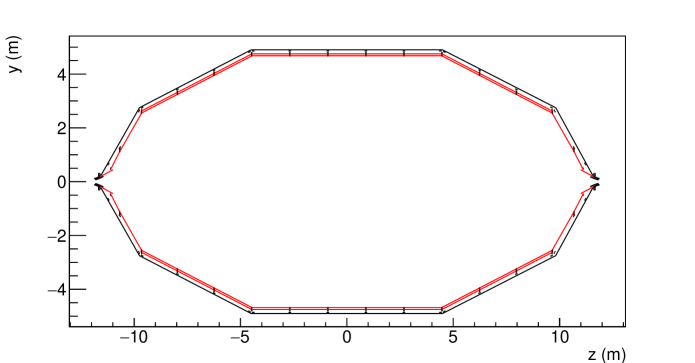
Figure 11: Schematic cross-sectional view of the KATRIN main spectrometer vessel (black, outside) and inner electrode system (red, inside).

Figure 12 presents the aspect ratio distribution of the two models (left: triangles, right: rectangles). One can see that especially the triangle model has many triangles with large (${\rm AR}>20$) aspect ratios. Figure 13 shows the distance ratio distributions for these two models for the central field point ${\bf P}=(0,0,0)$. Due to the large number of elements and the small element sizes (relative to typical field point – element distances), most of the distance ratio values are above 100, where the fast 7-point cubature method can be applied.

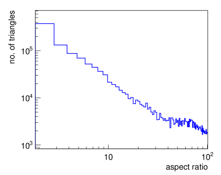
(a) Triangles

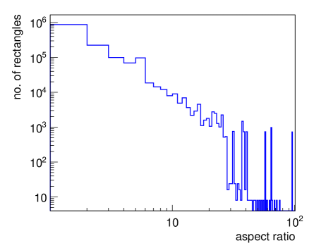
(b) Rectangles

Figure 12: Aspect ratio distribution of triangles (left) and rectangles (right) of our two discretization models of the KATRIN main spectrometer electrode system with electric dipole field. Vertical axis: number of elements per bin, with constant bin size 1.

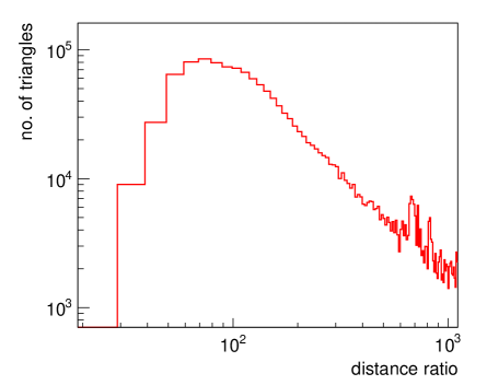
(a) Triangles

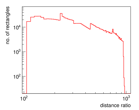
(b) Rectangles

Figure 13: Distance ratio distribution of triangles (left) and rectangles (right) of our two discretization models of the KATRIN main spectrometer electrode system with electric dipole field, at field point ${\bf P}=(0,0,0)$ (center of spectrometer). Vertical axis: number of elements per bin, with constant bin size 10.

The electrode discretization has been assembled with the software tool KGeoBag, which is a C++ library allowing to define arbitrary three-dimensional electrode geometries in a text file based on the Extensible Markup Language (XML) [19, 20, 22, 71]. The meshed geometry data, which contains also information on the applied electric potentials, can be automatically created from the input and transferred to the field computation program KEMField. The latter [19, 10] is a library, written in C++, which can solve electrostatic and magnetostatic problems with BEM. The electrostatics code part contains several logically separated classes which are responsible for

• computation of boundary integrals over single surface (mesh) elements;

• linear algebra routines for determining the charge densities by solving a linear algebraic equation system.

• Integrating field solver, and

• field solving with fast Fourier transform on multipoles (FFTM) [78, 79, 80].

KEMField profits from a very small memory footprint through usage of shell matrices that are not stored in memory, allowing to solve for arbitrary large equation systems with the Robin Hood iterative method [26]. Furthermore KEMField profits from libraries and computing languages, like MPI (Messaging Parsing Interface) [73] and OpenCL [74] in order to gain computation speed from parallel platforms like multi-core CPUs and highly parallel graphical processors.

With the computed charge density values, the electric potential and field at an arbitrary field point can be calculated by summing the potential and field contributions of the individual elements. In order to compare the relative errors of the various field computation methods, we generated randomly 3000 field points inside a cylinder with 9 m length and 3.5 m radius (centered at the KATRIN main spectrometer vessel center), and we computed the average of the relative errors defined in Secs. 2 and 4. As reference potential and field values, we used the Gauss-Legendre biquadrature method desribed in Sec. 2. Table 1 summarizes our results for two different analytical methods and for Gaussian cubature. In the case of triangles, we performed two calculations: first, with all triangles, and second, using only the small aspect ratio (${\rm AR}<10$) triangles (since we showed in Secs. 2 and 4 that both the analytical and the Gaussian cubature calculations for triangles are sensitive to the aspect ratio). One can see in table 1 the following features: a, the Gaussian cubature integration method has much smaller relative errors than both analytical integrations: the potential error is practically double precision, while the field error is somewhat larger, but also close to the double precision level; b, the analytical method 2 (Refs. [27, 28]) has smaller errors than the analytical method 1 (Refs. [19, 26]); c, the potential errors are in all cases smaller than the field errors; d, in case of using only smaller aspect ratio triangles, the errors are smaller than with all (i.e. also large aspect ratio) triangles. We mention here that we tried to reduce the potential and field rounding errors of the 1.5 million elements by Kahan summation [24, 75], but with no success.

In addition to the large relative potential and field errors, the analytical 1 method of Refs. [19, 26] has the following problem for the field computation of triangles: at some very sharply defined field points (e.g. ${\bf P}=(0,0,0)$) the relative field error is extremely large (more than 10), i.e. the field value is completely wrong, and in some cases one gets nan or inf results (with C++ compiler). Only a few triangles (from the 1.5 million) are responsible for these wrong field values (they have small – ${\rm AR}<10$ – aspect ratio).

Table 1: Average relative error of potential and field simulation of triangles and rectangles at 3000 field points, computed with two different analytical methods and with Gaussian cubature. Analytical 1: Refs. [19, 26]; Analytical 2: Refs. [27, 28].

	Analytical 1	Analytical 2	Gaussian cubature
Potential error (triangles)	$7.1\cdot 10^{-9}$	$4.6\cdot 10^{-12}$	$4.9\cdot 10^{-16}$
Field error (triangles)	$1.8\cdot 10^{-6}$	$3.2\cdot 10^{-9}$	$4.5\cdot 10^{-14}$
Potential error (triangles, ${\rm AR}<10$)	$1.8\cdot 10^{-11}$	$2.0\cdot 10^{-12}$	$3.2\cdot 10^{-16}$
Field error (triangles, ${\rm AR}<10$)	$1.4\cdot 10^{-7}$	$6.7\cdot 10^{-10}$	$2.4\cdot 10^{-14}$
Potential error (rectangles)	$2.6\cdot 10^{-11}$	$1.7\cdot 10^{-11}$	$1.1\cdot 10^{-16}$
Field error (rectangles)	$6.3\cdot 10^{-7}$	$5.2\cdot 10^{-9}$	$1.7\cdot 10^{-14}$

6 Computation time with CPU and GPU

In this section, we compare the computer speed of the Gaussian cubature and the analytical integration methods on CPU (C++) and GPU (OpenCL) [74, 76]. For this purpose, we calculated the electric potential and field of the 2 electrode models described in the previous section and containing 1.5 million triangles and 1.5 million rectangles, respectively. Table 2 presents the CPU computation time values for 100 field points and five different calculation types: two analytical (Refs. [27, 28, 19, 26]) and three Gaussian cubature methods. At the cubature method, the Gaussian points are calculated from the individual element geometry before each potential / field calculation. One can see that the Gaussian cubature methods (especially those with 7 and 12 points) are significantly faster than the analytical calculations. The computation time of the Gaussian cubature formulas increases almost linearly with the number of Gaussian points. The triangle and the rectangle integrations have approximately the same speed.

Table 2: Computation time values and speed increase factors (relative to analytical speed) for cubature implementation on CPU, with field and potential of 1.5 million triangles and rectangles computed at 100 field points. Analytical 1: Refs. [19, 26]; Analytical 2: Refs. [27, 28]. SF1: (time of analytical 1)/time; SF2: (time of analytical 2)/time.

Element type	Computation method	Time (s)	SF1	SF2
Triangles	Analytical 1	161	1	0.44
	Analytical 2	70	2.3	1
	7-point cubature	15.7	10.3	4.5
	12-point cubature	25.5	6.3	2.7
	33-point cubature	61	2.6	1.1
Rectangles	Analytical 1	140	1	0.56
	Analytical 2	79	1.8	1
	7-point cubature	18	7.7	4.4
	12-point cubature	28	5.1	2.8
	33-point cubature	70	2.0	1.1

Table 3 shows the time comparisons on a GPU with OpenCL, with two different analytical methods (Refs. [27, 28, 19, 26]) and with a distance ratio dependent cubature integrator incorporating the 7-point, 12-point and 33-point cubature methods. Also on this platform the cubature is much faster than analytical methods and can deliver a speed up of almost an order of magnitude for triangles.

Table 3: Computation time values and speed factors for cubature implementation on GPU, with field and potential computed at 10000 field points. Analytical 1: Refs. [19, 26]; Analytical 2: Refs. [27, 28]. In the case of distance ratio dependent computation the 7-point, 12-point and the 33-point cubature methods and the analytical method 2 are used.

Element type	Computation method	Time (s)	Speed increase factor
			(relative to analytical 1)
Rectangles	Analytical 1	82.7	1
	Analytical 2	81.7	1.01
	7-point cubature	27.8	3
	Distance ratio dependent	64.8	1.3
Triangles	Analytical 1	258	1
	Analytical 2	80.2	3.2
	7-point cubature	28.3	9.1
	Distance ratio dependent	97	2.7

We investigated also a possible time benefit by saving the Gaussian points for all elements into heap memory in advance. The storage of the Gaussian points can require a lot of memory (e.g.: 800 MB for 5 million element and 7 points for each element), depending from the meshed input geometry. In the following we compare the 7-point and 12-point cubature against the analytical method as discussed in [27]. As shown in table 4, again we gather a speed increase up to factor five by using the Gaussian cubature versus the analytical 2 method of [27]. Since the Gaussian points are computed on the fly in the fast stack memory, the non-cached variant of our code is only marginally slower than the code version with precomputed Gaussian points.

Table 4: Speed test with 1.5 Million triangles, 100 field points, precomputed vs. non-precomputed Gaussian points.

Computation method	Time (s)	Speed increase factor
		(relative to analytical 2)
Analytical 2	60.7	1
7-point cubature, precomputed	12.7	4.8
7-point cubature, non-precomputed	14.5	4.2
12-point cubature, precomputed	19.9	3
12-point cubature, non-precomputed	23	2.6

We recognized that the Gaussian cubature computation time depends very much on implementation details. In the C++ codes of the above described calculations we used double arrays for the representation of the Gaussian point, field point and electric field components. In another calculation, we used the TVector3 class of the ROOT data analysis code package [72]. The code layout is more elegant and clean by using the TVector3 class, but in this case the computation is four times slower than by using double arrays. Interestingly, the cubature computation is about two times slower even if the TVector3 commands are inside the C++ functions but they are not used for the calculations.

GPU architectures profit from a high degree of parallelism, even though the clock speed is not that high as on CPUs. In order to guarantee a highly parallel execution of the code, the used data fragments may not be too large, hence we have to avoid large double arrays, because using too large data arrays results in a lower degree of parallelism (and hence less speed) (e.g. for the 33-point cubature the array containing the Gaussian points is 99-dimensional). This is why we focused on avoiding saving data in large arrays due to limitation of register memory on GPU chips. Instead, we are using mostly single double values achieving a very highly parallel execution of the code.

At the end of this section, we present a few technical details about the computers and codes that we used. We run all our single-threaded C++ code on an Intel Xeon CPU with 3.10 GHz clock speed (E5-2687W v3). All CPU programs have been compiled with GCC 4.8.4 with optimization flag O3. Our code has been ported to OpenCL (version 1.1) as well. In order to test the speed on GPUs, we use a Tesla K40c card running at 875 MHz.

7 Conclusions

Integration over triangles and rectangles is important for many applications of mathematics, science and engineering, especially for FEM and BEM. Analytical integration is believed to be more accurate than numerical integration. Nevertheles, in some special cases the latter one has higher accuracy and also higher speed. We demonstrated in our paper that in the case of electric potential and field calculation of charged triangles and rectangles at points far from these elements the Gaussian cubature numerical integration method is much more accurate and faster than some of the best analytical integration methods. Using the Gaussian cubature method, the triangles and rectangles with continuous charge distribution are replaced by discrete point charges, the potential and field of which can be computed by simple formulas. At field points far from the elements, the analytical methods have large rounding errors, while the accuracy of the Gaussian cubature method is limited only by computer arithmetic precision. Closer to the elements, a Gaussian cubature formula with higher number of Gaussian points (nodes) has to be employed, in order to get the maximal accuracy. Very close to the elements, the Gaussian cubature method is not precise enough, therefore analytical integration has to be used there. Nevertheless, for a typical BEM problem the field point is far from most of the elements, therefore the simple, fast and accurate Gaussian cubature method can be used for a large majority of the boundary elements.

The complex electrode examples described in Sec. 5 illustrate that the Gaussian cubature method can be four to seven orders of magnitude more accurate than some of the best analytical methods that can be found in the literature. In addition, the examples in Sec. 6 show that the potential and field computation with Gaussian cubature can be three to ten times faster than the analytical methods, both with CPU and with GPU. An additional advantage of the Gaussian cubature method is that accurate higher derivatives of the electric field can be relatively easily calculated analytically by point charges, while in the case of analytical integrations this is a rather difficult task. The higher derivatives can be useful for field mapping computations in conjunction with the Hermite interpolation method.

In our paper, we compared the Gaussian cubature method with analytical integration in the case of constant BEM elements (i.e. elements with constant charge density). Nevertheless, the Gaussian cubature method can be easily applied also for elements with arbitrary charge density function (e.g. linear, quadratic etc.). Most probably, the Gaussian cubature method is more accurate and faster than analytical integration also in the case of higher order charge density functions. We conjecture that the Gaussian cubature method presented in our paper for electrostatics can also be applied for magnetostatics and time-dependent electromagnetic problems. E.g. magnetic materials can be computed by fictive magnetic charges, and the magnetic field in that case can be calculated by similar formulas than electric field of electric charges. It might be that the Gaussian cubature numerical integration method can also be used for the efficient computation of multipole moment coefficients of triangles and rectangles (see Ref. [80] for analytical integration results). The ten different Gaussian cubature formulas presented in our paper can be used for arbitrary high-precision and fast integrations over triangles and rectangles.

Acknowledgments

We are grateful to Prof. J. Formaggio, Dr. T. J. Corona and J. Barrett for many fruitful discussions, especially on the comparisons of the numerical results against the analytical method of Refs. [27, 28], and we thank Prof. J. Formaggio and J. Barrett for their reading the manuscript and important comments. Furthermore, we thank Prof. G. Drexlin for his continuous support of this dedicated project. D. Hilk would like to thank the Karlsruhe House Of Young Scientists (KHYS) for a research travel grant to the Laboratory of Nuclear Science at MIT in order to work on the cubature implementation on graphical processors together with Prof. Joseph Formaggio and John Barrett. We acknowledge the support of the German Helmholtz Association HGF and the German Ministry for Education and Research BMBF (05A14VK2 and 05A14PMA).

Appendix A Gaussian points and weights for triangles

Table A1: Barycentric coordinates and weights of the 4-point (degree 3) Gaussian cubature for triangle. See Refs. [41, 45, 46].

$\lambda_{A}$	$\lambda_{B}$	$\lambda_{C}$	weight
1/3	1/3	1/3	-9/16
3/5	1/5	1/5	25/48
1/5	3/5	1/5	25/48
1/5	1/5	3/5	25/48

Table A2: Barycentric coordinates and weights of the 7-point (degree 5) Gaussian cubature for triangle; $t=1/3$, $s=(1-\sqrt{15})/7$, $r=(1+\sqrt{15})/7$. Both the second and the third row corresponds to three Gaussian points with equal weights, according to all possible different permutations of $\lambda_{A}$ and $\lambda_{B}=\lambda_{C}$ (like the rows two to four in Table A1). From Refs. [44, 47, 41], [43] (p. 420).

$\lambda_{A}$	$\lambda_{B}$	$\lambda_{C}$	weight
$t$	$t$	$t$	9/40
$t+2ts$	$t-ts$	$t-ts$	$(155+\sqrt{15})/1200$
$t+2tr$	$t-tr$	$t-tr$	$(155-\sqrt{15})/1200$

Table A3: Barycentric coordinates and weights of the 12-point (degree 7) Gaussian cubature for triangle. Each row corresponds to three Gaussian points with equal weights: we get the second and third points by the permutations $(\lambda_{A},\lambda_{B},\lambda_{C})\to(\lambda_{B},\lambda_{C},\lambda_{A})$ and $(\lambda_{A},\lambda_{B},\lambda_{C})\to(\lambda_{C},\lambda_{A},\lambda_{B})$, respectively; taken from Ref. [48].

$\lambda_{A}$	$\lambda_{B}$	$\lambda_{C}$	weight
0.06238226509439084	0.06751786707392436	0.8700998678316848	0.05303405631486900
0.05522545665692000	0.3215024938520156	0.6232720494910644	0.08776281742889622
0.03432430294509488	0.6609491961867980	0.3047265008681072	0.05755008556995056
0.5158423343536001	0.2777161669764050	0.2064414986699949	0.13498637401961758

Table A4: Barycentric coordinates and weights of the 19-point (degree 9) Gaussian cubature for triangle. Each of the rows two to five corresponds to three Gaussian points with equal weights, according to all possible different permutations of $\lambda_{A}$ and $\lambda_{B}=\lambda_{C}$ (like in Table A1). The last row corresponds to six Gaussian points with equal weights, according to all possible permutations of $\lambda_{A}$, $\lambda_{B}$ and $\lambda_{C}$. Numbers taken from Ref. [49].

$\lambda_{A}$	$\lambda_{B}$	$\lambda_{C}$	weight
1/3	1/3	1/3	0.09713579628279610
0.02063496160252593	0.48968251919873704	0.48968251919873704	0.03133470022713983
0.1258208170141290	0.4370895914929355	0.4370895914929355	0.07782754100477543
0.6235929287619356	0.18820353561903219	0.18820353561903219	0.07964773892720910
0.9105409732110941	0.04472951339445297	0.04472951339445297	0.02557767565869810
0.03683841205473626	0.7411985987844980	0.22196298916076573	0.04328353937728940

Table A5: Barycentric coordinates and weights of the 33-point (degree 12) Gaussian cubature for triangle. Each of the first five rows corresponds to three Gaussian points with equal weights, according to all possible different permutations of $\lambda_{A}$ and $\lambda_{B}=\lambda_{C}$ (like in Table A1). Each of the last three rows corresponds to 6 Gaussian points with equal weights, according to all possible permutations of $\lambda_{A}$, $\lambda_{B}$ and $\lambda_{C}$. Numbers taken from Ref. [50].

$\lambda_{A}$	$\lambda_{B}$	$\lambda_{C}$	weight
0.4570749859701478	0.27146250701492611	0.27146250701492611	0.06254121319590276
0.1197767026828138	0.44011164865859310	0.44011164865859310	0.04991833492806094
0.0235924981089169	0.48820375094554155	0.48820375094554155	0.02426683808145203
0.7814843446812914	0.10925782765935432	0.10925782765935432	0.02848605206887754
0.9507072731273288	0.02464636343633558	0.02464636343633558	0.00793164250997364
0.1162960196779266	0.2554542286385173	0.62824975168355610	0.04322736365941421
0.02303415635526714	0.2916556797383410	0.68531016390639186	0.02178358503860756
0.02138249025617059	0.1272797172335894	0.85133779251024000	0.01508367757651144

Appendix B Gaussian points and weights for rectangles

Table B1: Natural coordinates and weights of the 4-point (degree 3) Gaussian cubature for rectangle; $s=1/\sqrt{3}$. From Refs. [43] (p. 417), [51] (p. 8).

$x$	$y$	weight
s	s	1/4
s	-s	1/4
-s	s	1/4
-s	-s	1/4

Table B2: Natural coordinates and weights of the 7-point (degree 5) Gaussian cubature for rectangle; $t=\sqrt{14/15}$, $r=\sqrt{3/5}$, $s=\sqrt{1/3}$. The last row corresponds to 4 Gaussian points with equal weights, according to all possible sign changes (like in Table B1): $(x,y)\to\;(r,s),\,(r,-s),\,(-r,s),\,(-r,-s)$. From Refs. [41] (p. 246), [44] (p. 298), [51] (p. 9).

$x$	$y$	weight
0	0	2/7
0	t	5/63
0	-t	5/63
r	s	5/36

Table B3: Natural coordinates and weights of the 12-point (degree 7) Gaussian cubature for rectangle; $r=\sqrt{6/7}$, $s=\sqrt{(114-3\sqrt{583})/287}$, $t=\sqrt{(114+3\sqrt{583})/287}$, $B_{1}=49/810$, $B_{2}=(178981+2769\sqrt{583})/1888920$, $B_{3}=(178981-2769\sqrt{583})/1888920$. Each of the last two rows corresponds to four Gaussian points with equal weights, according to all possible sign changes of $s$ and $t$, like in Tables B1 and B2. From Refs. [41] (p. 253), [52] (p. 403).

$x$	$y$	weight
r	0	$B_{1}$
-r	0	$B_{1}$
0	r	$B_{1}$
0	-r	$B_{1}$
s	s	$B_{2}$
t	t	$B_{3}$

Table B4: Natural coordinates and weights of the 17-point (degree 9) Gaussian cubature for rectangle. Each of the last four rows corresponds to four Gaussian points with equal weights, according to the transformations $(x,y)\to\;\pm(x,y),\;\pm(-y,x)$ (rotations by $0^{\circ}$, $180^{\circ}$ and $\pm 90^{\circ}$ in the $x-y$ plane). From Refs. [53] (p. 194), [42] (p. 257), [43] (p. 419).

$x$	$y$	weight
0	0	0.131687242798353921
0.968849966361977720	0.630680119731668854	0.022219844542549678
0.750277099978900533	0.927961645959569667	0.028024900532399120
0.523735820214429336	0.453339821135647190	0.099570609815517519
0.076208328192617173	0.852615729333662307	0.067262834409945196

Table B5: Natural coordinates and weights of the 33-point (degree 13) Gaussian cubature for rectangle. Each of the last eight rows corresponds to four Gaussian points with equal weights, according to the transformations $(x,y)\to\;\pm(x,y),\;\pm(-y,x)$ (rotations by $0^{\circ}$, $180^{\circ}$ and $\pm 90^{\circ}$ in the $x-y$ plane). From Ref. [54] (p. 145).

$x$	$y$	weight
0	0	0.075095528857806335
0.778809711554419422	0.983486682439872263	0.007497959716124783
0.957297699786307365	0.859556005641638928	0.009543605329270918
0.138183459862465353	0.958925170287534857	0.015106230954437494
0.941327225872925236	0.390736216129461000	0.019373184633276336
0.475808625218275905	0.850076673699748575	0.029711166825148901
0.755805356572081436	0.647821637187010732	0.032440887592500675
0.696250078491749413	0.070741508996444936	0.053335395364297350
0.342716556040406789	0.409304561694038843	0.064217687370491966

References

- [1] K. H. Huebner, The Finite Element Method for Engineers, J. Wiley & Sons, New York, 1975.
- [2] L. J. Segerlind, Applied Finite Element Analysis, J. Wiley & Sons, New York, 1984.
- [3] R. D. Cook et al., Conceps and Applications of Finite Element Analysis, J. Wiley & Sons, New York, 1989.
- [4] O. P. Gupta, Finite and Boundary Element Methods in Engineering, A. A. Balkema Publishers, Rotterdam Brookfield, 1999.
- [5] P. K. Kythe, An Introduction to the Boundary Element Method, CRC Press, London Tokyo, 1995.
- [6] L. Gaul, M. Kögl and M. Wagner, Boundary Element Methods for Engineers and Scientists, Springer-Verlag, Berlin, 2003.
- [7] G. Beer, I. Smith and Ch. Duenser, The Boundary Element Method with Programming, Springer, Wien New York, 2008.
- [8] C. A. Brebbia, J. C. F. Telles and L. C. Wrobel, Boundary Element Techniques, Springer-Verlag, Berlin, 1984.
- [9] C. A. Brebbia and J. Dominguez, Boundary Elements An Introductory Course, McGraw-Hill Comp. , New York, 1992.
- [10] T. J. Corona, Tools for Electromagnetic Field Simulation in the KATRIN Experiment, Master thesis, MIT, 2009.
- [11] M. Szilágyi, Electron and Ion Optics, Plenum Press, New York and London, 1988.
- [12] P. W. Hawkes and E. Kasper, Principles of Electron Optics, Vol 1, Academic Press, Harcourt Brace Jovanovich, 1989.
- [13] Ch. Kraus et al., Final results from phase II of the Mainz neutrino mass search in tritium decay, Eur. Phys. J. C, Vol. 40, 447, 2005.
- [14] V. M. Lobashev, The search for the neutrino mass by direct method in the tritium beta-decay and perspectives of study it in the project KATRIN, Nucl. Phys. A, Vol. 719, 153c, 2003.
- [15] F. Glück et al., The neutron decay retardation spectrometer aSPECT: Electromagnetic design and systematic effects, Eur. Phys. J. A, Vol. 23, 135, 2005; S. Baessler et al., First measurements with the neutron decay spectrometer aSPECT, Eur. Phys. J. A, Vol. 38, 17, 2008.
-
[16]
J. Angrik et al. (KATRIN Collaboration), KATRIN Design Report 2004,
Wissenschaftliche Berichte FZKA 7090.
http://bibliothek.fzk.de/zb/berichte/FZKA7090.pdf. - [17] M. Prall et al., The KATRIN pre-spectrometer at reduced filter energy, New Journal of Physics 14 (2012) 073054.
- [18] M. Arenz et al., Commissioning of the vacuum system of the KATRIN Main Spectrometer, J. Instrum. 11, P04011, 2016.
- [19] T. J. Corona, Methodology and Application of High Performance Electrostatic Field Simulation in the KATRIN Experiment, PhD thesis, Chapel Hill, 2014.
- [20] D. Furse, Techniques for Direct Neutrino Mass Measurement Utilizing Tritium -Decay, PhD dissertation, MIT, 2015.
- [21] S. Groh, Modeling of the response function and measurement of transmission properties of the KATRIN experiment, PhD dissertation, KIT, 2015.
- [22] S. Groh et al., Kassiopeia: A Modern, Extensible C++ Particle Tracking Package, to be published.
- [23] M. V. K. Chari and S. J. Salon, Numerical Methods in Electromagnetism, Academic Press, San Diego, 2000.
- [24] Ch. W. Ueberhuber, Numerical Computation Vol. 1, Methods, Software and Analysis, Springer, Berlin, 1997.
- [25] D. Goldberg, What every computer scientist should know about floating-point arithmetic, ACM Computing Surveys 23, 5-48, 1991.
- [26] J. Formaggio et al., Solving for micro- and macro-scale electrostatic configurations using the Robin Hood algorithm, Progress In Electromagnetics Research B 39, 1-37, 2011.
- [27] I. Hänninen, M. Taskinen, and J. Sarvas, Singularity subtraction integral formulae for surface integral equations with rwg, rooftop and hybrid basis functions, Progress In Electromagnetics Research 63, 243–278, 2006.
- [28] D. Hilk, Investigation and removal of stored background electrons with the electric dipole method in the KATRIN main spectrometer, PhD thesis, KIT, 2016.
- [29] S. M. Rao et al., A simple numerical solution procedure for statics problems involving arbitrary-shaped surfaces, IEEE Transactions on Antennas and Propagation 27, 604-608, 1979.
- [30] E. E. Okon and R. F. Harrington, The potential due to a uniform source distribution over a triangular domain, International Journal for Numerical Methods in Engineering 18, 1401-1419, 1982.
- [31] K. Davey and S. Hinduja, Analytical integration of linear three-dimensional triangular elements in BEM, Applied Mathematical Modelling 13, 450-461, 1989.
- [32] A. Tatematsu, S. Hamada and T. Takuma, Analytical Expressions of Potential and Electric Field Generated by a Triangular Surface Charge with a High-Order Charge Density Distribution, Electrical Engineering in Japan 139, 9-17, 2002.
- [33] S. Mukhopadhyay and N. Majumdar, Use of Triangular Elements for Nearly Exact BEM Solutions, arXiv:0704.1563 [math.NA]
- [34] S. Lopez-Pena, A. G. Polimeridis, and J. R. Mosig, On the analytic-numeric treatment of weakly singular integrals on arbitrary polygonal domains, Progress In Electromagnetics Research, Vol. 117, 339-355, 2011.
- [35] M. J. Carley, Analytical Formulae for Potential Integrals on Triangles, Journal of Applied Mechanics 80, 041008, 1-7, 2013.
- [36] E. Durand, Electrostatique, Vol. I, Masson et Cie, 1964.
- [37] M. Eupper, Eine verbesserte Integralgleichungsmethode zur numerischen Lösung dreidimensionaler Dirichletprobleme und ihre Anwendung in der Elektronenoptik, PhD thesis, Tübingen, 1985.
- [38] A. B. Birtles, B. J. Mayo and A. W. Bennett, Computer technique for solving 3-dimensional electron-optics and capacitance problems, Proc. IEE 120, 213-220, 1973. Erratum: Proc. IEE 120, 559, 1973.
- [39] G. Evans, Practical Numerical Integration, John Wiley & Sons, Chichester, 1993.
- [40] P. K. Kythe and M. R. Schäferkotter, Handbook of Computational Methods for Integration, Chapman& Hall/CRC, London, 2005.
- [41] A. H. Stroud, Approximate Calculation of Multiple Integrals, Prentice Hall Inc., New Jersey (1971).
- [42] H. Engels, Numerical Quadrature and Cubature, Academic Press, London, 1980.
- [43] G. Engeln-Müllges and F. Uhlig, Numerical Algorithms with C, Springer, 1996.
- [44] J. Radon, Zur mechanischen Kubatur, Monatsh. Math. 52, 286-300, 1948.
- [45] P. C. Hammer and A. H. Stroud, Numerical Integration Over Simplexes, Math. Tables Aids Comput. 10, 137-139, 1956.
- [46] P. C. Hammer and A. H. Stroud, Numerical Evaluation of Multiple Integrals II, Math. Tables Aids Comput. 12, 272-280, 1958.
- [47] P. C. Hammer, O. J. Marlowe and and A. H. Stroud, Numerical Integration Over Simplexes and Cones, Math. Tables Aids Comput. 10, 130-137, 1956.
- [48] K. Gatermann, The construction of symmetric cubature formulas for the square and the triangle, Computing 40, 229-240, 1988.
- [49] J. N. Lyness and D. Jespersen, Moderate Degree Symmetric Quadrature Rules for the Triangle, J. Inst. Maths. Applics 15, 19-32, 1975.
- [50] S. Papanicolopulos, Computation of moderate-degree fully-symmetric cubature rules on the triangle using symmetric polynomials and algebraic solving, Computers and Mathematics with Applications 69, 650-666, 2015.
- [51] J. Albrect and L. Collatz, Zur numerischen Auswertung mehrdimensionaler Integrale, Zeitschrift für Angewandte Mathematik und Mechanik 38, 1-15, 1958.
- [52] G. W Tyler, Numerical integration of functions of several variables, Canad. J. Math. 5, 393-412, 1953.
- [53] H. M. Möller, Kubaturformeln mit minimaler Knotenzahl, Numer. Math. 25, 185-200, 1976.
- [54] R. Cools and A. Haegemans, Another step forward in searching for cubature formulae with a minimal number of knots for the square, Computing 40, 139-146, 1988.
- [55] P. Rabinowitz and N. Richter, Perfectly Symmetric Two-Dimensional Integration Formulas with Minimal Numbers of Points, Mathematics of Computation 23, 765-779, 1969.
- [56] I. P. Omelyan and V. B. Solovyan, Improved cubature formulae of high degrees of exactness for the square, Journal of Computational and Applied Mathematics 188, 190–204, 2006.
- [57] D. A. Dunavant, High degree efficient symmetrical gaussian quadrature rules for the triangle, International Journal for Numerical Methods in Engineering 21, 1129-1148, 1985.
- [58] A. Haegemans and R. Piessens, Construction of Cubature Formulas of Degree Eleven for Symmetric Planar Regions, Using Orthogonal Polynomials, Numer. Math. 25, 139-148, 1976.
- [59] A. Haegemans and R. Piessens, Construction of Cubature Formulas of Degree Seven and Nine Symmetric Planar Regions, Using Orthogonal Polynomials, SIAM Journal on Numerical Analysis 14, 492-508, 1977.
- [60] M. E. Laursen and M. Gellert, Some criteria for numerically integrated matrices and quadrature formulas for triangles, International Journal for Numerical Methods in Engineering 12, 67-76, 1978.
- [61] S. Wandzura and H. Xiao, Symmetric quadrature rules on a triangle, Computers and Mathematics with Applications 45, 1829-1840, 2003.
- [62] L. Zhang, T. Cui and H. Liu, A set of symmetric quadrature rules on triangles and tetrahedra, Journal of Computational Mathematics 27, 89–96, 2009.
- [63] R. Cools and P. Rabinowitz, Monomial cubature rules since “Stroud”: a compilation, Journal of Computational and Applied Mathematics 48, 309-326, 1993.
- [64] J. N. Lyness and R. Cools, A Survey of Numerical Cubature over Triangles, Preprint MCS-P410-0194, Argonne National Laboratory, 1994.
- [65] R. Cools, Monomial cubature rules since Stroud: a compilation – part 2, Journal of Computational and Applied Mathematics 112, 21-27, 1999.
- [66] R. Cools, Advances in multidimensional integration, Journal of Computational and Applied Mathematics 149, 1–12, 2002.
- [67] R. Cools, An encyclopaedia of cubature formulas, Journal of Complexity 19, 445–453, 2003.
- [68] R. Cools, Encyclopaedia of Cubature Formulas, web page
- [69] M. G. Duffy, Quadrature Over a Pyramid or Cube of Integrands with a Singularity at a Vertex, SIAM J. Numer. Anal. 19, 1260-1262, 1982.
- [70] K. Valerius, The wire electrode system for the KATRIN main spectrometer, Prog. Part. Nucl. Phys. 64, 291-293, 2010.
- [71] R. Combe, Design optimization of the KATRIN transport section and investigation of related background contribution. Master thesis, KIT, 2015.
- [72] ROOT Data Analysis Framework, C++ program package, developed in CERN. https://root.cern.ch/
- [73] D. W. Walker and J. J. Dongarra, MPI: a standard message passing interface. Supercomputer, 12, 56-68, 1996.
- [74] E. Stone, D. Gohara, and G. Shi, OpenCL: A parallel programming standard for heterogeneous computing systems, Computing in science and engineering, 12, 66-72, 2010.
- [75] W. Kahan, Further remarks on reducing truncation errors, Communications of the ACM 8, 40-40, 1965.
- [76] Wen-mei W. Hwu (Editor), GPU Computing Gems, Jade edition, Morgan Kaufmann, 1. edition, 2011.
- [77] S. Stern, Untersuchung der Untergrundeigenschaften des KATRIN Hauptspektrometers mit gepulsten elektrischen Dipolfeldern, Bachelor Thesis, KIT, 2016.
- [78] J. Barrett, PhD thesis, MIT, 2016
- [79] W. Gosda, A new Preconditioning Approach using the Fast Fourier Transformation on Multipoles, Diploma Thesis, KIT, 2015.
- [80] J. Barrett, J. Formaggio and T. J. Corona, A method to calculate the spherical multipole expansion of the electrostatic charge distribution on a triangular boundary element, Progress In Electromagnetics Research B 63, 123-143, 2015.