TRex: A Tomography Reconstruction Proximal Framework for Robust Sparse View X-Ray Applications

Abstract

We present TRex, a flexible and robust Tomographic Reconstruction framework using proximal algorithms. We provide an overview and perform an experimental comparison between the famous iterative reconstruction methods in terms of reconstruction quality in sparse view situations. We then derive the proximal operators for the four best methods. We show the flexibility of our framework by deriving solvers for two noise models: Gaussian and Poisson; and by plugging in three powerful regularizers. We compare our framework to state of the art methods, and show superior quality on both synthetic and real datasets.

I Introduction

Reducing the dosage in X-ray tomography is a very important issue in medical applications, since long term exposure to X-rays can have adverse health effects. This can be done in at least two ways: (a) reducing the X-ray beam power, which leads to increased measurement noise at the detectors; or (b) acquiring fewer projections to reduce the acquisition time [1]. This makes the reconstruction problem even more ill-posed, since less information is collected from the volume to be reconstructed; and one has to use non-linear regularizers (priors) to achieve a reasonable result. This is typically done using iterative solvers [2, 3].

Iterative algorithms for X-ray tomography reconstruction have been around for years. In fact, one of the first implemented tomography reconstruction algorithm was an iterative one [4, 5, 6]. However, non-iterative, transform-based algorithms, such as the filtered back projection (FBP) [7, 8, 9], have been more popular due to their speed and low computational cost. Moreover, most commercial X-ray CT scanners employ some variant of FBP in their reconstruction software [10]. Recently, interest has been ignited again in iterative algorithms because, although they are more computationally demanding, they are much more flexible and yield superior reconstruction quality by employing powerful priors.

Thus, in this work, we study iterative reconstruction techniques. We present TRex, a flexible proximal framework for robust X-Ray tomography reconstruction in sparse view applications. TRex uses iterative algorithms, especially the SART (Simultaneous ART) [11, 12], to solve the tomography proximal operator. We show that they are better suited for this task and produce better performance than state of the art, combined with different noise models in the data terms and with different powerful regularizers. Up to our knowledge, this is the first time these methods have been used to directly solve the tomography proximal operator.

We start by conducting a thorough comparison of the famous iterative algorithms including SART [11], ART (Algebraic Reconstruction Technique) [11], SIRT (Simultaneous Iterative Reconstruction Technique) [13], BSSART (Block Simplified SART) [14], BICAV (Block Iterative Component Averaging) [15], Conjugate Gradient (CG) [16], and OS-SQS (Ordered Subset-Separable Quadratic Surrogates) [17, 18, 19, 20, 21]. We establish that SART provides the best performance in the sparse view measurements situations, followed closely by ART, OS-SQS, and BICAV.

We then describe our framework, TRex, which is based on using proximal algorithms [22, 23] together with these iterative methods. We derive proximal operators for SART, ART, BICAV, and OS-SQS. We show how to use these proximal operators to minimize two data fitting terms: (a) least squares (LS) that assumes a Gaussian noise model; and (b) weighted least squares (WLS) that assumes an approximation to a Poisson noise model [24]. We also show how to plug in different powerful regularizers; namely Isotropic Total Variation (ITV) [25], Anisotropic Total Variation (ATV) [26], and Sum of Absolute Differences (SAD) [27]. We perform thorough comparisons between the different proximal operators, data terms, and regularizers using real and synthetic data.

Finally, we compare our framework to state of the art methods, namely the ADMM method from Ramani et al. [28] and the OS-SQS method (with and without momentum method) from Kim et al. [29], and show that our framework gives superior reconstruction quality. Please consult [30] for further details, expanded experiments, and more results.

In summary, we provide the following contributions:

1. We present TRex, a flexible proximal reconstruction framework that relies on iterative methods for directly solving the tomography proximal operator.

2. We perform a thorough experimental comparison of famous iterative reconstruction methods on synthetic and real datasets.

3. We derive proximal operators for SART, ART, BICAV, and OS-SQS; and compare them.

4. We derive solvers for different data terms assuming different noise models, namely Gaussian and Poisson models, using the derived proximal operators, and show how to use our framework with different powerful regularizers.

5. We compare our framework to state of the art methods and show that it produces superior reconstructions.

6. We make our code—which is based on the ASTRA toolbox [31]—and data publicly available at https://github.com/mohamedadaly/TRex.

This paper is organized as follows. In Sec. II we present related work. An overview of the famous iterative algorithms is detailed in Sec. III. The different proximal operators are derived in Sec. IV. The TRex framework is explained in Sec. V, where we show the general algorithm together with three regularizers and two data terms. The experiments and datasets are presented in Sec. VI, and finally the conclusions are given in Sec. VII.

II Related Work

There are two general approaches for X-ray tomography reconstruction: transform-based methods and iterative methods [4, 1]. Transform methods rely on the Radon transform and its inverse introduced in 1917. The most widely used reconstruction method is the Filtered Backprojection (FBP) algorithm introduced [1, 4]. Transform methods are usually viewed as much faster than iterative methods, and have therefore been the method of choice for X-ray scanner manufacturers [10].

Iterative methods, on the other hand, use algebraic techniques to solve the reconstruction problem. They generally model the problem as a linear system and solve it using established numerical methods [1]. ART, and its many variants, are among the best known iterative reconstruction algorithms [5, 32, 33, 34, 11, 12]. They use variations of the projection method of Kaczmarz [35] and have modest memory requirements, and have been shown to yield better reconstruction results than transform methods. They are matrix free, and work without having to explicitly store the system matrix. OS-SQS and related methods [17, 19, 20] are closely related to ART and have similar properties to SIRT [36]. They have also been shown [29] to be accelerated using momentum techniques.

Iterative methods provide more flexibility in incorporating prior information into the reconstruction process. For example, instead of assuming a Gaussian noise model and minimizing a least squares data term, one can easily use iterative methods with other noise models, such as the Poisson noise model [24, 17, 37, 38, 2] that boils down to solving WLS problem instead. Priors are also easy to use with iterative methods. For example, the Total Variation [25] prior has been used for tomography reconstruction [39, 40].

Proximal algorithms have been widely used in many problems in machine learning and signal processing [41, 42, 22, 23]. They have also been used in tomography reconstruction [40, 39]. For example, [40] used the Alternating Direction Method of Multipliers (ADMM) [22] with total variation prior, where the data term was optimized using CG [16]. [26] discussed using the Chambolle-Pock algorithm [43] for tomography reconstruction with different priors. [28] used ADMM with Preconditioned CG (PCG) [44] for optimizing the weighted least squares data term. [21] used Linearized ADMM [23] (also known as Inexact Split Uzawa [45]) with Ordered Subset-based methods [19] for optimizing the data term and FISTA [46] for optimizing the prior term. However, none of these methods used the iterative algorithms we study in this work as their data term solver, which provides superior reconstruction as we will show.

There are currently a number of open source software packages for tomography reconstruction. SNARK09 [47] is one of the oldest. The Reconstruction ToolKit (RTK) [48] is a high performance C++ toolkit focusing on 3D cone beam reconstruction that is based on the image processing package Insight ToolKit (ITK). It includes implementations of several algorithms, including FDK, SART, and an ADMM TV-regularized solver with CG [40]. The ASTRA toolbox [31] is a Matlab-based GPU-accelerated toolbox for tomography reconstruction. It includes implementations of several algorithms, including SART, SIRT, FBP, among others. We modify and extend ASTRA to implement our algorithms and generate the experiments in this work.

III Iterative Algorithms

Algorithm 1 Outline of Iterative Algorithms

1:$A\in\mathbb{R}{}^{m\times n}$, $\alpha\in\mathbb{R}$, $p\in\mathbb{R}{}^{m}$

2:Initialize: $x^{(0)}$

3:for all $t=1\ldots T$  do

4:     for all subsets $S\in\mathcal{S}$  do

5:         $x^{(t+1)}=x^{(t)}+\alpha\Delta x^{(t)}$

6:         $x^{(t+1)}=\mbox{clip}(x^{(t+1)})$

7:     end for

8:end forreturn volume reconstruction $x\in\mathbb{R}{}^{n}$

The tomography problem can be represented as solving a linear system [4, 1]

$$Ax=p,$$ (1)

where $x\in\mathbb{R}^{n}$ is the unknown volume in vector form, $A\in\mathbb{R}^{m\times n}$ is the projection system matrix, and $p\in\mathbb{R}^{m}$ represents the measured line projections (sinogram). The iterative algorithms that we study in this work all have the same general outline in Alg. 1, but differ in the update formula in step 4. The subset $S$ in step 3 can be only 1 projection ray as in ART i.e. there are $m$ subsets $S_{i}=\{i\,|\,i=1\ldots m\}$; can contain all the rays in a projection view as in SART i.e. there are $m/s$ subsets where $s$ is the number of projection views; or can contain the whole projection rays as in SIRT i.e. there is only one subset $S=\{1,\ldots,m\}$. Step 5 clips the negative values of the volume, which is assumed to be non-negative.

The update step $\Delta x^{(t)}$ is typically a function of (a subset of) the forward projection error $p_{S}-A_{S}x^{(t)}$ that is then back projected with some normalization procedure. It can take the form

$$\Delta x^{(t)}=\Phi\left(A_{S}^{T},p_{S}-A_{S}x^{(t)}\right)$$

where the function $\Phi(\cdot)$ computes the required update, $A_{S}$ contains a subset of the rows of $A$, similarly for $p_{S}$–please see below. This can be seen as an approximation to the actual gradient $A^{T}(p-Ax)$ of the least square objective

$$\operatorname*{arg\,min}_{x}\|Ax-p\|_{2}^{2}$$

and so these algorithms can be viewed as variations of (stochastic) gradient descent [29] where they differ on how they approximate the gradient. We also notice that the inner loop in step 3 for all these algorithms takes roughly the same time, since it involves one full sweep over the rows of $A$.

Below we quickly review the different methods, and Table I provides a summary of their important properties.

Method	Update Step	Subset	Solved Problem	Converges
ART [5]	$\begin{aligned} x_{j}^{(t+1)}&=x_{j}^{(t)}+\alpha\frac{p_{i}-\sum_{k}a_{ik}x_{k}^{(t)}}{\sum_{k}a_{ik}^{2}}a_{ij}\\ x^{(t+1)}&=x^{(t)}+\alpha A_{i}^{T}R^{-1}\left(p_{i}-A_{i}x^{(t)}\right)\end{aligned}$	one ray	$\begin{aligned} x^{\star}=&\operatorname*{arg\,min}_{x}\|x\|_{2}^{2}\\ &\operatorname*{s.t.\,}Ax=p\end{aligned}$	Yes
SIRT [13]	$\begin{aligned} x_{j}^{(t+1)}&=x_{j}^{(t)}+\alpha\frac{1}{\sum_{i=1}^{m}a_{ij}}\sum_{i=1}^{m}\frac{p_{i}-\sum_{k=1}^{n}a_{ik}x_{k}^{(t)}}{\sum_{k=1}^{n}a_{ik}}a_{ij}\\ x^{(t+1)}&=x^{(t)}+\alpha C^{-1}A^{T}R^{-1}\left(p-Ax^{(t)}\right)\end{aligned}$	all rays	$x^{\star}=\operatorname*{arg\,min}_{x}\|Ax-p\|_{R^{-1}}^{2}$	Yes
SART [11]	$\begin{aligned} x_{j}^{(t+1)}&=x_{j}^{(t)}+\alpha\frac{1}{\sum_{i\in S}a_{ij}}\sum_{i\in S}\frac{p_{i}-\sum_{k=1}^{n}a_{ik}x_{k}^{(t)}}{\sum_{k=1}^{n}a_{ik}}a_{ij}\\ x^{(t+1)}&=x^{(t)}+\alpha C_{S}^{-1}A_{S}^{T}R^{-1}\left(p-A_{S}x^{(t)}\right)\end{aligned}$	one view	$\begin{aligned} x^{\star}\approx&\operatorname*{arg\,min}_{x}\|x\|_{2}^{2}\\ &\operatorname*{s.t.\,}Ax=p\end{aligned}$	No
BSSART [14]	$\begin{aligned} x_{j}^{(t+1)}&=x_{j}^{(t)}+\alpha\frac{1}{\sum_{i=1}^{m}a_{ij}}\sum_{i\in S}\frac{p_{i}-\sum_{k=1}^{n}a_{ik}x_{k}^{(t)}}{\sum_{k=1}^{n}a_{ik}}a_{ij}\\ x^{(t+1)}&=x^{(t)}+\alpha C^{-1}A_{S}^{T}R^{-1}\left(p_{S}-A_{S}x^{(t)}\right)\end{aligned}$	one view	$\begin{aligned} x^{\star}=&\operatorname*{arg\,min}_{x}\|x\|_{2}^{2}\\ &\operatorname*{s.t.\,}Ax=p\end{aligned}$	Yes
BICAV [15]	$\begin{aligned} x_{j}^{(t+1)}&=x_{j}^{(t)}+\alpha\frac{1}{\sum_{i\in S}\{a_{ij}\neq 0\}}\sum_{i\in S}\frac{p_{i}-\sum_{k=1}^{n}a_{ik}x_{k}^{(t)}}{\sum_{k=1}^{n}a_{ik}^{2}}a_{ij}\\ x^{(t+1)}&=x^{(t)}+\alpha C_{S}^{-1}A_{S}^{T}R^{-1}\left(p_{S}-A_{S}x^{(t)}\right)\end{aligned}$	one view	$\begin{aligned} x^{\star}=&\operatorname*{arg\,min}_{x}\|x\|_{2}^{2}\\ &\operatorname*{s.t.\,}Ax=p\end{aligned}$	Yes
OS-SQS [19]	$\begin{aligned} x_{j}^{(t+1)}&=x_{j}^{(t)}+\frac{\alpha s}{\left(\sum_{k=1}^{m}a_{kj}\sum_{i=1}^{n}a_{ki}\right)}\sum_{i\in S}\left(p_{i}-\sum_{k=1}^{n}a_{ik}x_{k}^{(t)}\right)a_{ij}\\ x^{(t+1)}&=x^{(t)}+\alpha sC^{-1}A_{S}^{T}\left(p_{S}-A_{S}x^{(t)}\right)\end{aligned}$	one view	$x^{\star}\approx\|Ax-p\|_{2}^{2}$	No
CGLS [16, 44]	$x^{(t+1)}=x^{(t)}+\alpha_{t}\Phi\left(A^{T}(p-Ax^{(t)})\right)$	all rays	$x^{\star}=\|Ax-p\|_{2}^{2}$	Yes

Table I: Summary of iterative methods and their properties. The first line in the update step is voxel-based, while the second is the matrix formulation. See Sec. III for details.

III-1 ART

[5, 6] is the first algebraic method, and is based on Kaczmarz alternating projection algorithm [35]. ART treats each row of $A$ in turn, and updates the current estimate according to

$$x_{j}^{(t+1)}=x_{j}^{(t)}+\alpha\frac{p_{i}-\sum_{k}a_{ik}x_{k}^{(t)}}{\sum_{k}a_{ik}^{2}}a_{ij}\mbox{ for }i=1\ldots m,$$

where $x_{j}^{(t)}$ is the $j$th voxel at time $t$, $a_{ij}$ is the entry in the $i$th row and $j$th column of $A$ and $\alpha\in\mathbb{R}$ is the relaxation parameter. This update is performed once for each row of $A$, and one iteration includes a full pass over all the $m$ rows. The term $\sum_{k}a_{ik}x_{k}^{(t)}$ is the forward projection of the volume estimate for the $i$th ray (equation or row), the difference in the numerator is the projection error, that is then back projected by multiplying the transpose of the $i$th row. It has been shown that ART converges to a least-norm solution to the consistent system of equations [49] i.e. it solves

$$x^{\star}=\operatorname*{arg\,min}_{x}\|x\|_{2}^{2}\operatorname*{s.t.\,}Ax=p.$$ (2)

In matrix notation, this can be also expressed as

$$x^{(t+1)}=x^{(t)}+\alpha A_{i}^{T}R^{-1}\left(p_{i}-A_{i}x^{(t)}\right)$$

where $A_{i}\in\mathbb{R}^{n}$ is the $i$th row of $A$ and $R\in\mathbb{R}^{m\times m}=\operatorname{diag}(r_{i})$ is a diagonal matrix where $r_{i}=\sum_{j}a_{ij}^{2}=\|A_{i}\|_{2}^{2}$ is the squared-norm of the $i$th row $A_{i}$.

III-2 SIRT

[13] performs the updates simultaneously i.e. updates the volume once instead of updating it per each row $A_{i}$. The update equation becomes

$$x_{j}^{(t+1)} = x_{j}^{(t)}+\alpha\frac{1}{\sum_{i=1}^{m}a_{ij}}\sum_{i=1}^{m}\frac{p_{i}-\sum_{k=1}^{n}a_{ik}x_{k}^{(t)}}{\sum_{k=1}^{n}a_{ik}}a_{ij}.$$

In matrix form this becomes

$$x^{(t+1)}=x^{(t)}+\alpha C^{-1}A^{T}R^{-1}\left(p-Ax^{(t)}\right)$$

where $C\in\mathbb{R}^{n\times n}=\operatorname{diag}(c_{j})$ is a diagonal matrix where $c_{j}=\sum_{i}a_{ij}$ is the sum of column $j$ of $A$ and $R=\operatorname{diag}(r_{i})$ where $r_{i}=\sum_{j}a_{ij}$ is the sum of row $i$ of $A$. In each iteration, SIRT performs a full forward projection $Ax^{(t)}$, computes the residual, and then back projects it. The diagonal matrices $R$ and $C$ perform scaling for the relevant entries. It has been shown [14, 50] that SIRT converges to a solution of the WLS problem

$$x^{\star}=\operatorname*{arg\,min}_{x}\|Ax-p\|_{R^{-1}}^{2}=\min_{x}(Ax-p)^{T}R^{-1}(Ax-p)$$ (3)

for $0<\alpha<2$. SIRT has been shown [36] to be closely related, and in fact quite equivalent in terms of convergence properties, to the OS-SQS method. It has also been shown to converge best for $\alpha=2-\epsilon$ for a small $0<\epsilon\ll 1$.

III-3 SART

[11] is a tradeoff between ART and SIRT, in that it updates the volume after processing all the rows in a particular projection view. The update equation becomes

$$x_{j}^{(t+1)} = x_{j}^{(t)}+\alpha\frac{1}{\sum_{i\in S}a_{ij}}\sum_{i\in S}\frac{p_{i}-\sum_{k=1}^{n}a_{ik}x_{k}^{(t)}}{\sum_{k=1}^{n}a_{ik}}a_{ij}$$

for $S\in\mathcal{S}$ where the summation $i\in S$ is across all rows (rays) in projection view $S$ for all views $\mathcal{S}$. This has been shown to provide faster convergence than ART and better reconstruction results than SIRT [51, 52]. In matrix form it becomes

$$x^{(t+1)}=x^{(t)}+\alpha C_{S}^{-1}A_{S}^{T}R^{-1}\left(p_{S}-A_{S}x^{(t)}\right)$$

where $A_{S}\in\mathbb{R}^{s\times n}$ contains the $s$ rows in projection $S$, $p_{S}$ contains the corresponding $s$ rays from the projection measurements, $R$ contains the row sums as in SIRT, while $C_{S}=\operatorname{diag}(c_{j}^{S})$ contains the column sums restricted to the rows in $S$ i.e. $c_{j}^{S}=\sum_{i\in S}a_{ij}$. There is still no proof of convergence for SART in the literature, but there are proofs for variants of SART, such as BSSART and BICAV below, that converge to a minimum-norm solution like ART. This motivates us to assume that SART solves approximately the least norm problem in Eq. 2.

III-4 BSSART

[14] is a slight simplification of SART, where the column sums in the update equation are done over all the rows of $A$ instead of just over the rows in the current view, which is quite similar to SIRT. The update equation becomes

$$x_{j}^{(t+1)} = x_{j}^{(t)}+\alpha\frac{1}{\sum_{i=1}^{m}a_{ij}}\sum_{i\in S}\frac{p_{i}-\sum_{k=1}^{n}a_{ik}x_{k}^{(t)}}{\sum_{k=1}^{n}a_{ik}}a_{ij}$$

for $S\in\mathcal{S}$ , which provides a slight speedup since the column sums are now independent of the iteration. The matrix formulation becomes

$$x^{(t+1)}=x^{(t)}+\alpha C^{-1}A_{S}^{T}R^{-1}\left(p_{S}-A_{S}x^{(t)}\right)$$

where the diagonal matrices are both independent of the projection view $S$ as in SIRT. BSSART has been shown [14] to converge to the minimum norm solution

$$x^{\star}=\operatorname*{arg\,min}_{x}\|x\|_{2}^{2}\operatorname*{s.t.\,}Ax=p$$

as ART for $0<\alpha<2$.

III-5 BICAV

[15, 14] is another closely-related algorithm to SART. It updates the volume after each projection view according to

$$x_{j}^{(t+1)} = x_{j}^{(t)}+\alpha\frac{1}{c_{j}^{S}}\sum_{i\in S}\frac{p_{i}-\sum_{k=1}^{n}a_{ik}x_{k}^{(t)}}{\sum_{k=1}^{n}a_{ik}^{2}}a_{ij}$$

for $S\in\mathcal{S}$ where $c_{j}^{S}=\sum_{i\in S}\{a_{ij}\neq 0\}$ and $\{a_{ij}\neq 0\}=1$ when $a_{ij}$ is non-zero is 0 otherwise. The difference from SART is that it computes the squared norm of the rows of $A$ and counts the number of non-zero entries in the columns of $A$. The matrix formulation is

$$x^{(t+1)}=x^{(t)}+\alpha C_{S}^{-1}A_{S}^{T}R^{-1}\left(p_{S}-A_{S}x^{(t)}\right)$$

where now $r_{i}=\sum_{j}a_{ij}^{2}=\|A_{i}\|_{2}^{2}$ and $C_{S}=\operatorname{diag}(c_{j}^{S})$. It is shown [14] that BICAV converges to the minimum-norm solution

$$\min_{x}\|x\|^{2}\operatorname*{s.t.\,}Ax=p$$

for $0<\alpha<2$.

III-6 OS-SQS

[19, 29] is closely related to SART. It is usually derived from a majorization-minimization perspective [17, 19, 20, 29], but with a specific choice of surrogate functions and parameters [20] the update equation becomes

$$x_{j}^{(t+1)} = x_{j}^{(t)}+\alpha\frac{s}{c_{j}}\sum_{i\in S}\left(p_{i}-\sum_{k=1}^{n}a_{ik}x_{k}^{(t)}\right)a_{ij}$$

for $S\in\mathcal{S}$ where $s$ is the number of subsets $S$ in $\mathcal{S}$ (number of inner iterations), $c_{j}=\left(\sum_{k=1}^{m}a_{kj}\sum_{i=1}^{n}a_{ki}\right)$, and in general the set $S$ can contain more than one projection view. In matrix form it becomes

$$x^{(t+1)}=x^{(t)}+\alpha sC^{-1}A_{S}^{T}\left(p_{S}-A_{S}x^{(t)}\right)$$

where the matrix $C=\operatorname{diag}(A^{T}A\mathbf{1}_{m})=\operatorname{diag}(c_{j})$ where $\mathbf{1}_{m}$ is the vector of $m$ ones. OS-SQS is a special case of the SQS method, which processes all the rows of $A$ at once like SIRT. Simultaneous SQS, i.e. without ordered subsets, has been shown [19] to converge to a least square solution

$$x^{\star}=\operatorname*{arg\,min}_{x}\|Ax-p\|_{2}^{2},$$ (4)

and a special case of relaxed OS-SQS converges, where the relaxation parameter becomes iteration-dependent and decreases over time [53]. However, OS-SQS with fixed $\alpha$ is not known to converge. Therefore, like SART, we assume that it solves the LS problem in Eq. 4 above approximately.

III-7 CGLS

[16, 44] is a type of Conjugate Gradient that solves the least squares normal equations directly. Like SIRT, it updates the constraint once per full sweep over the projection rays. The update equation in matrix notation is

$$x^{(t+1)}=x^{(t)}+\alpha_{t}\Phi(A^{T}(p-Ax^{(t)}))$$

where the update step is a function of the backprojection of the projection error, and the parameter $\alpha_{t}$ depends on the specific version of CGLS (here we use the Fletcher-Reeves update rule[16]). CGLS is proven to be convergent to the solution of the LS problem in Eq. 4.

$$x^{\star}=\operatorname*{arg\,min}_{x}\|Ax-p\|_{2}^{2}.$$

Note that the function $\Phi(\cdot)$ is more complicated than other iterative algorithms, and involves several steps with a couple of auxiliary variables [16].

IV Tomography Proximal Operators

Proximal algorithms are a class of optimization algorithms that are quite flexible and powerful [42, 22, 23]. They are generally used to efficiently solve non-smooth, constrained, distributed, or large scale optimization problems. They are more modular than other optimization problems, in the sense that they provide a few lines of code that depend on solving smaller conventional, and usually simpler, optimization problems called proximal operator. The proximal operator [41, 42, 23] for a function $h(\cdot)$ is a generalization of projections on convex sets, and can be thought of intuitively as getting closer to the optimal solution while staying close to the current estimate. Formally it is defined as

$$\operatorname{prox}_{\lambda h}(u)=\operatorname*{arg\,min}_{x}h(x)+\frac{1}{2\lambda}\|x-u\|_{2}^{2},$$ (5)

where $x,u\in\mathbb{R}^{n}$ and $\lambda$ is a regularization parameter. Many proximal operators of common functions are easy to compute, and often admit a closed form solution. Computing the proximal operator of a certain function opens the way to solving hard optimization problems involving this function and other regularization terms e.g. smoothing norms or sparsity inducing norms, which otherwise is not generally easy. We will derive tomography proximal operators for SART, ART, BICAV, and OS-SQS, where the objective is to solve

$$\mbox{prox}_{\lambda h}(u)=\operatorname*{arg\,min}_{x}\|Ax-p\|_{2}^{2}+\frac{1}{2\lambda}\|x-u\|_{2}^{2}.$$ (6)

Method	Update Step	Converges
ART [5]	$\begin{aligned} y_{i}^{(t+1)}&=y_{i}^{(t)}+\alpha\frac{\sqrt{2\lambda}p_{i}-\sqrt{2\lambda}\sum_{k}a_{ik}x_{k}^{(t)}-y_{i}^{(t)}}{2\lambda\sum_{k}a_{ik}^{2}+1}\mbox{ for }i\in S\\ x_{j}^{(t+1)}&=x_{j}^{(t)}+\alpha\frac{\sqrt{2\lambda}p_{i}-\sqrt{2\lambda}\sum_{k}a_{ik}x_{k}^{(t)}-y_{i}^{(t)}}{2\lambda\sum_{k}a_{ik}^{2}+1}\sqrt{2\lambda}a_{ij}\mbox{ for }j=1\ldots n\end{aligned}$	Yes
SART [11]	$\begin{aligned} y_{i}^{(t+1)}&=y_{i}^{(t)}+\alpha\frac{\sqrt{2\lambda}p_{i}-\sqrt{2\lambda}\sum_{k}a_{ik}x_{k}^{(t)}-y_{i}^{(t)}}{\sqrt{2\lambda}\sum_{k}a_{ik}+1}\mbox{ for }i\in S\\ x_{j}^{(t+1)}&=x_{j}^{(t)}+\alpha\frac{\sum_{i\in S}\frac{\sqrt{2\lambda}p_{i}-\sqrt{2\lambda}\sum_{k}a_{ik}x_{k}^{(t)}-y_{i}^{(t)}}{\sqrt{2\lambda}\sum_{k}a_{ik}+1}\sqrt{2\lambda}a_{ij}}{\sqrt{2\lambda}\sum_{i\in S}a_{ij}}\mbox{ for }j=1\ldots n\end{aligned}$	No
BICAV [15]	$\begin{aligned} y_{i}^{(t+1)}&=y_{i}^{(t)}+\alpha\frac{\sqrt{2\lambda}p_{j}-\sqrt{2\lambda}\sum_{k}a_{jk}x_{k}^{(t)}-y_{j}^{(t)}}{2\lambda\sum_{k}a_{jk}^{2}+1}\mbox{ for }i\in S\\ x_{j}^{(t+1)}&=x_{j}^{(t)}+\alpha\frac{\sum_{i\in S}\frac{\sqrt{2\lambda}p_{i}-\sqrt{2\lambda}\sum_{k}a_{ik}x_{k}^{(t)}-y_{i}^{(t)}}{2\lambda\sum_{k}a_{ik}^{2}+1}\sqrt{2\lambda}a_{ij}}{\sum_{i\in S}\{a_{ij}\neq 0\}}\mbox{ for }j=1\ldots n\end{aligned}$	Yes
OS-SQS [19]	$\begin{aligned} x_{j}^{(t+1)}&=x_{j}^{(t)}+\alpha\frac{s}{2\lambda c_{j}+1}\left(2\lambda\sum_{i\in S}(p_{j}-\sum_{k}a_{ik}x_{k}^{(t)})a_{ij}+u_{j}-x_{j}^{(t)}\right)\mbox{ for }j=1\ldots n\end{aligned}$	No

Table II: Summary of the proximal operators update steps. See Sec. IV for details.

IV-A SART, ART, and BICAV

They (approximately) solve the least-norm problem

$$x^{\star}=\operatorname*{arg\,min}_{x}\|x\|_{2}^{2}\operatorname*{s.t.\,}Ax=p.$$

What we want is a solver for Eq. 6. This is equivalent to solving

$$\min_{x}2\lambda\|Ax-p\|_{2}^{2}+\|x-u\|_{2}^{2}.$$ (7)

Introduce new variables $y=\sqrt{2\lambda}(p-Ax)$ and $z=x-u$. The problem becomes

$$\min_{y,z} \|y\|_{2}^{2}+\|z\|_{2}^{2}$$

$$\operatorname*{s.t.\,} y+\sqrt{2\lambda}Az=\sqrt{2\lambda}(p-Au).$$ (8)

Rewriting Eq. 8 we arrive at

$$\mbox{$\min$}_{y,z} \left\|\left[\begin{array}[]{c}y\\ z\end{array}\right]\right\|_{2}^{2}$$

subject to $$\left[\begin{array}[]{cc}I&\sqrt{2\lambda}A\end{array}\right]\left[\begin{array}[]{c}y\\ z\end{array}\right]=\sqrt{2\lambda}\left(p-Au\right)$$

which can be written as

$$\mbox{$\min$}_{\tilde{x}} \left\|\tilde{x}\right\|_{2}^{2}$$

$$\operatorname*{s.t.\,} \tilde{A}\tilde{x}=\tilde{p},$$

where $\tilde{x}\in\mathbb{R}^{m+n}$, $\tilde{A}\in\mathbb{R}^{m\times m+n}$, and $\tilde{p}\in\mathbb{R}^{m}$. This is now a consistent under-determined linear system, and can be solved using either ART, SART, or BICAV.

Although we introduced new variables $y$ and $z$ and increased the dimensionality of the problem from $n$ to $n+m$, we can solve the modified algorithm efficiently with very little computational overhead. Instead of solving explicitly for the optimal $y^{\star}$ and $z^{\star}$, we can manipulate the algorithm to solve directly for the optimal $x^{\star}.$ For example, for SART, the initialization and update equation for $\tilde{x}$ become

$$\tilde{x}_{j}^{(0)} = \mathbf{0},$$

$$\tilde{x}_{j}^{(t+1)} = \tilde{x}_{j}^{(t)}+\alpha\frac{\sum_{i\in\mathcal{S}}\frac{\tilde{p}_{i}-\sum_{k}\tilde{a}_{ik}\tilde{x}_{k}^{(t)}}{\sum_{k}\tilde{a}_{ik}}\tilde{a}_{ij}}{\sum_{i\in S}\tilde{a}_{ij}},$$ (11)

which can be expanded in terms of $y$, $z$, and $A$ as

$$y^{(0)} = \mathbf{0}_{m}$$

$$z^{(0)} = \mathbf{0}_{n}$$

$$y_{j}^{(t+1)} = y_{j}^{(t)}+\frac{\alpha\sum_{i\in\mathcal{S}}\frac{\tilde{p}_{i}-\sqrt{2\lambda}\sum_{k}a_{ik}z_{k}^{(t)}-y_{i}^{(t)}}{\sqrt{2\lambda}\sum_{k}a_{ik}+1}\delta_{ij}}{1},$$

$$z_{j}^{(t+1)} = z_{j}^{(t)}+\alpha\frac{\sum_{i\in\mathcal{S}}\frac{\tilde{p}_{i}-\sqrt{2\lambda}\sum_{k}a_{ik}z_{k}^{(t)}-y_{i}^{(t)}}{\sqrt{2\lambda}\sum_{k}a_{ik}+1}\sqrt{2\lambda}a_{ij}}{\sqrt{2\lambda}\sum_{i\in S}a_{ij}},$$

where $\delta_{ij}=1$ when $i=j$ and 0 otherwise. Using the fact that $z=x-u$ and $\tilde{p}_{i}=\sqrt{2\lambda}p_{i}-\sqrt{2\lambda}\sum_{k}a_{ik}u_{k}$ and simplifying we arrive at

$$y^{(0)} = \mathbf{0}_{m}$$

$$x^{(0)} = u$$

$$y_{j}^{(t+1)} = y_{j}^{(t)}+\alpha\sum_{i\in S}\frac{\sqrt{2\lambda}p_{i}-\sqrt{2\lambda}\sum_{k}a_{ik}x_{k}^{(t)}-y_{i}^{(t)}}{\sqrt{2\lambda}\sum_{k}a_{ik}+1}\delta_{ij},$$

$$x_{j}^{(t+1)} = x_{j}^{(t)}+\alpha\frac{\sum_{i\in S}\frac{\sqrt{2\lambda}p_{i}-\sqrt{2\lambda}\sum_{k}a_{ik}x_{k}^{(t)}-y_{i}^{(t)}}{\sqrt{2\lambda}\sum_{k}a_{ik}+1}\sqrt{2\lambda}a_{ij}}{\sqrt{2\lambda}\sum_{i\in S}a_{ij}}.$$

Following the same line of reasoning, we can arrive at similar update formulas for both ART and BICAV. The steps are summarized in Table II. Alg. 2 provides an outline of the proximal operator.

Algorithm 2 SART, ART, and BICAV Proximal Operator

1:$A\in\mathbb{R}{}^{m\times n}$, $\alpha,\lambda\in\mathbb{R}$, $p\in\mathbb{R}{}^{m}$, $u\in\mathbb{R}^{n}$

2:Initialize:

$$x^{(0)} =u$$

$$y^{(0)} =\mathbf{0}_{m}$$

3:for all $t=1\ldots T$  do

4:     for all subsets $S\in\mathcal{S}$  do

5:         Update according to Table II:

$$x_{j}^{(t+1)} =x_{j}^{(t)}+\alpha\Delta x_{j}^{(t)}\mbox{ for }j=1\ldots n$$

$$y_{i}^{(t+1)} =y_{i}^{(t)}+\alpha\Delta y_{i}^{(t)}\mbox{ for }i\in S$$

6:         $x^{(t+1)}=\mbox{clip}(x^{(t+1)})$

7:     end for

8:end forreturn $x^{\star}=\operatorname*{arg\,min}_{x}\|Ax-p\|_{2}^{2}+\frac{1}{2\lambda}\|x-u\|_{2}^{2}$

IV-B OS-SQS

We want to express the proximal operator problem

$$\operatorname{prox}_{\lambda h}(u)=\operatorname*{arg\,min}_{x}h(x)+\frac{1}{2\lambda}\|x-u\|_{2}^{2}$$

in the form of the LS problem that can be solved (approximately) by OS-SQS i.e.

$$x^{\star}=\operatorname*{arg\,min}_{x}\|Ax-p\|_{2}^{2}.$$

Rewrite as

$$\operatorname*{arg\,min}_{x}2\lambda\|Ax-p\|_{2}^{2}+\|x-u\|_{2}^{2},$$

which is equivalent to

$$\operatorname*{arg\,min}_{x}\left\|\left[\begin{array}[]{c}\sqrt{2\lambda}A\\ I\end{array}\right]x-\left[\begin{array}[]{c}\sqrt{2\lambda}p\\ u\end{array}\right]\right\|_{2}^{2}$$

$$\iff\operatorname*{arg\,min}_{x}\left\|\tilde{A}x-\tilde{p}\right\|_{2}^{2}$$

where

$$\tilde{A} = \left[\begin{array}[]{c}\sqrt{2\lambda}A\\ I\end{array}\right]\in\mathbb{R}^{m+n\times n}$$

$$\tilde{p} = \left[\begin{array}[]{c}\sqrt{2\lambda}p\\ u\end{array}\right]\in\mathbb{R}^{m+n}.$$

The weighting matrix $\tilde{C}\in\mathbb{R}^{n\times n}$ now becomes

$$\tilde{C} = \mbox{diag}(\tilde{A}^{T}\tilde{A}\mathbf{1})$$

$$= \mbox{diag}\left((2\lambda A^{T}A+I)\mathbf{1}\right)$$

$$= \mbox{diag}\left(2\lambda A^{T}A\mathbf{1}+\mathbf{1}\right)$$

and its diagonal entries are

$$\tilde{c}_{j}=2\lambda c_{j}+1.$$

Write the matrix update equation in terms of $\tilde{A}$ and $\tilde{p}$ as

$$x^{(t+1)} =x^{(t)}+\alpha s\tilde{C}^{-1}\tilde{A}_{S}^{T}\left(\tilde{p}_{S}-\tilde{A}_{S}x^{(t)}\right)$$

$$=x^{(t)}+\alpha s\tilde{C}^{-1}\left[\begin{smallmatrix}\sqrt{2\lambda}A_{S}^{T}&I\end{smallmatrix}\right]\left[\begin{smallmatrix}\sqrt{2\lambda}(p_{S}-A_{S}x^{(t)})\\ u-x^{(t)}\end{smallmatrix}\right]$$

$$=x^{(t)}+\alpha s\tilde{C}^{-1}{\scriptstyle\left(2\lambda A_{S}^{T}(p_{S}-A_{S}x^{(t)})+(u-x^{(t)})\right)}.$$

In component form it becomes

$$x_{j}^{(t+1)} =x_{j}^{(t)}+\alpha\frac{s}{\tilde{c}_{j}}{\scriptstyle\left(2\lambda\sum_{i\in S}(p_{j}-\sum_{k}a_{ik}x_{k}^{(t)})a_{ij}+u_{j}-x_{j}^{(t)}\right)}.$$

The steps are summarized in Table II. Alg. 3 gives an outline.

Algorithm 3 OS-SQS Proximal Operator

1:$A\in\mathbb{R}{}^{m\times n}$, $\alpha,\lambda\in\mathbb{R}$, $p\in\mathbb{R}{}^{m}$, $u\in\mathbb{R}^{n}$

2:Initialize:

$$x^{(0)} =\mathbf{0}_{n}$$

3:for all $t=1\ldots T$  do

4:     for all subsets $S\in\mathcal{S}$  do

5:         $x_{j}^{(t+1)}=x_{j}^{(t)}+\alpha\Delta x_{j}^{(t)}\mbox{ for }j=1\ldots n$ according to Table II.

6:         $x^{(t+1)}=\mbox{clip}(x^{(t+1)})$

7:     end for

8:end forreturn $x^{\star}=\operatorname*{arg\,min}_{x}\|Ax-p\|_{2}^{2}+\frac{1}{2\lambda}\|x-u\|_{2}^{2}$

V TRex Proximal Framework

V-A Proximal Algorithm

The overall problem we want to solve is a regularized data fitting problem, namely

$$\operatorname*{arg\,min}_{x}f(x)+g(Kx),$$ (14)

where $f(\cdot)$ is a data fitting term that measures how much the solution fits the data and that depends on the measurement noise model assumed, $K\in\mathbb{R}^{d\times n}$ is a matrix, and $g(\cdot)$ is a regularization term that imposes constraints on acceptable solutions. We will use the Linearized ADMM method [22, 23] (also known as Inexact Split Uzawa [45, 54] or Proximal ADMM [55, 56, 57, 58]), for solving this problem for different data terms and different regularizers.

It rewrites Eq. 14 into the equivalent form

$$\operatorname*{arg\,min}_{x,z} f(x)+g(z)$$

$$\operatorname*{s.t.\,} Kx=z,$$

writes out the scaled augmented Lagrangian function [23]

$$\mathcal{L}_{\rho}(x,z,y)=f(x)+g(z)+\frac{\rho}{2}\|Kx-z+y\|_{2}^{2},$$

and then applies alternating minimization for the variables $x,$ $z$, and $y$ in turn:

$$x^{(t+1)} =\operatorname*{arg\,min}_{x}f(x)+\frac{\rho}{2}\|Kx-z^{(t)}+y^{(t)}\|^{2}$$

$$z^{(t+1)} =\operatorname*{arg\,min}_{z}g(z)+\frac{\rho}{2}\|Kx^{(t+1)}-z+y^{(t)}\|^{2}$$

$$y^{(t+1)} =y^{(t)}+Kx^{(t+1)}-z^{(t+1)}.$$

The problem with the $x$ step is that it contains the quadratic term $\|Kx\|^{2}=x^{T}K^{T}Kx$ in the minimization makes it hard to minimize since it’s not straightforward. We can cancel out that term by adding the following proximal term that makes it strongly convex and keeps the solution close to the previous iteration

$$\frac{1}{2}\|x-x^{k}\|_{S}^{2}=\frac{1}{2}(x-x^{k})^{T}S(x-x^{k})$$

to the objective fundtion where the special matrix $S$ is

$$S=\frac{1}{\mu}I-\rho K^{T}K$$

and this gives the modified $x$ step

$$x^{(t+1)} = \operatorname*{arg\,min}_{x}f(x)+\frac{\rho}{2}\|Kx-z^{(t)}+y^{(t)}\|^{2}+$$

$$\frac{1}{2}\|x-x^{(t)}\|_{S}^{2}$$

$$= \operatorname*{arg\,min}_{x}f(x)+\frac{\rho}{2}\|Kx\|^{2}-\rho\langle Kx,z^{(t)}-y^{(t)}\rangle+$$

$$\frac{1}{2}(x-x^{(t)})^{T}S(x-x^{(t)})$$

$$= \operatorname*{arg\,min}_{x}f(x)+\frac{\rho}{2}\|Kx\|^{2}-\rho\langle x,K^{T}(z^{(t)}-y^{(t)})\rangle+$$

$$\frac{1}{2}\|x\|_{S}^{2}-\langle x,Sx^{(t)}\rangle$$

$$= \operatorname*{arg\,min}_{x}f(x)+$$

$$\frac{1}{2\mu}\|x-\mu\rho K^{T}(z^{(t)}-y^{(t)})-\mu Sx^{(t)}\|^{2}$$

$$= \operatorname*{arg\,min}_{x}f(x)+$$

$$\frac{1}{2\mu}\|x-x^{(t)}-\mu\rho K^{T}\left(z^{(t)}-y^{(t)}-Kx^{(t)}\right)\|^{2}$$

which is simply the proximal operator of $f(x)$ with input $x^{(t)}+\mu\rho\left(z^{(t)}-u^{(t)}-K^{T}Kx^{(t)}\right)$ i.e. the iterations now become

$$x^{(t+1)} =\operatorname{prox}_{\mu f}\left(x^{(t)}+\mu\rho K^{T}\left(z^{(t)}-y^{(t)}-Kx^{(t)}\right)\right)$$

$$z^{(t+1)} =\operatorname{prox}_{\rho^{-1}g}\left(Kx^{(t+1)}+y^{(t)}\right)$$

$$y^{(t+1)} =y^{(t)}+Kx^{(t+1)}-z^{(t+1)}.$$

The algorithm is convergent for any $\rho>0$ and $\mu>\nicefrac{{1}}{{\rho\|K\|^{2}}}$ [23, 21]. The steps are summarized in Alg. 4. This framework is very flexible, and we will show how to solve for different data terms and different regularizers.

Algorithm 4 Linearized ADMM

1:$K\in\mathbb{R}{}^{d\times n}$, $\rho,\mu\in\mathbb{R}$ such that $\mu\rho\|K\|^{2}<1$, initial values $x^{(0)}\in\mathbb{R}^{n}$ and $z^{(0)}\in\mathbb{R}^{d}$

2:Initialize $y^{(0)}=\mathbf{0}_{d}$

3:for all $t=1\ldots T$  do

4:     $x^{(t+1)}=\mbox{prox}_{\mu f}\left(x^{(t)}-\rho\mu K^{T}(Kx^{(t)}-z^{(t)}+y^{(t)})\right)$

5:     $z^{(t+1)}=\mbox{prox}_{\rho^{-1}g}\left(Kx^{(t+1)}+y^{(t)}\right)$

6:     $y^{(t+1)}=y^{(t)}+Kx^{(t+1)}-z^{(t+1)}$

7:end forreturn $x^{(T)}=\operatorname*{arg\,min}_{x}f(x)+g(Kx)$

V-B Data Terms

We will consider the following data fidelity terms, which correspond to specific noise models:

V-B1 Gaussian Noise

Assume the measurements $p_{i}\forall i=1,\ldots m$ follow the model

$$p_{i}=a_{i}^{T}x+\varepsilon_{i}$$ (15)

where the noise $\varepsilon\sim\mathbb{N}(0,\sigma^{2})$ follows a Gaussian distribution. Maximizing the projection data log-likelihood

$$\mathcal{L}_{\text{G}}(p)\propto-\sum_{i}\left(p_{i}-a_{i}^{T}x\right)^{2}$$ (16)

is equivalent to minimizing the LS $\ell_{2}$ norm data term

$$f_{\text{G}}(x)=\|Ax-p\|_{2}^{2}=\sum_{i=1}^{m}(A_{i}^{T}x-p_{i})^{2}.$$ (17)

We can solve proximal operator $\operatorname{prox}_{\lambda f_{\text{G}}}(\cdot)$ directly using any of the algorithms from Table II.

V-B2 Poisson Noise

It can be shown that assuming an approximated Poisson noise model leads to a WLS data term, where the weights are proportional to the detector measurements [24, 17, 37, 2]. Indeed, the actual measurements produced by the X-ray CT scanner represent X-ray photon energy reaching the detector as compared to the energy leaving the X-ray gun. These are related to each other and to the linear attenuation coefficient according to Beer-Lambert law [59]:

$$I_{t}=I_{o}e^{-\int\mu(l)dl}$$

where $I_{t}$ is the transmitted intensity as measured by the detector, $I_{o}$ is the emitted intensity from the source, $\mu(l)$ is the linear attenuation coefficient of the material as a function of length $l$. The exponent represents the line integrals (projection data) we are dealing with. In particular, assuming that the X-ray photons are monochromatic (have only one single energy) i.e. ignoring beam hardening, the projection line integral data at detector $i$ is obtained from the physical measurements as

$$p_{i}=-\ln\frac{I_{t}^{i}}{I_{o}^{i}}$$ (18)

where $I_{t}^{i}$ is the intensity measured by detector $i$ and $I_{o}^{i}$ is the emitted intensity. The detector measurements are stochastic in nature, and assuming a Poisson distribution with mean $I_{o}^{i}\exp(-p_{i})$ we get

$$I_{t}^{i}\sim\mathbb{P}(I_{o}^{i}e^{-p_{i}})\approx\mathbb{P}(I_{o}^{i}e^{-A_{i}^{T}x}).$$

Using the ML approach, we maximize the log-likelihood of the measured data:

$$\mathcal{L}_{P}(x)=\sum_{i}I_{t}^{i}\ln\left(I_{o}^{i}e^{-A_{i}^{T}x}\right)-I_{o}^{i}e^{-A_{i}^{T}x}=\sum_{i}\phi_{i}\left(A_{i}^{T}x\right)$$ (19)

where

$$\phi_{i}(q)=I_{t}^{i}\ln\left(I_{o}^{i}e^{-q}\right)-I_{o}^{i}e^{-q}.$$

Applying a second-order Taylor’s expansion for $\phi_{i}(q)$ around an estimate of the $i$th line integral $p_{i}$ from Equation 18 [37]:

$$\phi_{i}(q) \approx\phi_{i}(p_{i})+\frac{d\phi_{i}}{dq}(p_{i})(q-p_{i})+\frac{1}{2}\frac{d^{2}\phi_{i}}{dq^{2}}(p_{i})(q-p_{i})^{2}$$

$$=(I_{t}^{i}\ln I_{t}^{i}-I_{t}^{i})-\frac{I_{t}^{i}}{2}(q-p_{i})^{2}$$

The first term is independent of $q$ and can be dropped (since we are interested in minimizing $\mathcal{L}_{P}(x)$). Substituting in Equation 19, we end up with the approximated log-likelihood

$$\mathcal{L}_{\text{G}}(x)\approx-\sum_{i}\frac{I_{t}^{i}}{2}\left(A_{i}^{T}x-p_{i}\right)^{2}=-\sum w_{i}\left(A_{i}^{T}x-p_{i}\right){}^{2}$$ (20)

where $w_{i}$ is the weight for projection measurement $i$ and is proportional to the measurement of the incident X-ray intensity on detector $i$ i.e. $w_{i}\propto I_{t}^{i}.$ Typically, the weights $w_{i}$ are normalized to have a maximum of 1, and we could apply any non-decreasing mapping on $w_{i}$, e.g. the square root, before feeding into the optimization problem, see Sec. VI-C.

Maximizing the likelihood is equivalent to minimizing the WLS data term

$$f_{\text{P}}(x)=\|Ax-p\|_{W}^{2}=\sum_{i=1}^{m}w_{i}(a_{i}^{T}x-p_{i})^{2}$$ (21)

where $\|x\|_{W}=x^{T}Wx$ and $W=\operatorname{diag}(w_{i})\in\mathbb{R}^{m\times m}$ is a diagonal matrix containing weights for each measurement.

We can solve the proximal operator

$$\operatorname{prox}_{\lambda f_{\text{P}}}(u)=\min_{x}\|Ax-p\|_{W}^{2}+\frac{1}{2\lambda}\|x-u\|^{2}$$ (22)

as follows. Define $\tilde{p}\in\mathbb{R}^{m}$ and $\tilde{A}\in\mathbb{R}^{m\times n}$ as

$$\tilde{p} = W^{\frac{1}{2}}p$$

$$\tilde{A} = W^{\frac{1}{2}}A$$

where $W^{\frac{1}{2}}=\operatorname{diag}\left(\sqrt{w_{i}}\right).$ We get

$$\|\tilde{A}x-\tilde{p}\|_{2}^{2} = (\tilde{A}x-\tilde{p})^{T}(\tilde{A}x-\tilde{p})$$

$$= \left(W^{\frac{1}{2}}(Ax-p)\right)^{T}\left(W^{\frac{1}{2}}(Ax-p)\right)$$

$$= (Ax-p)^{T}W^{\frac{1}{2}}W^{\frac{1}{2}}(Ax-p)$$

$$= \|Ax-p\|_{W}^{2}.$$

Now this is in the form that can be solved with the algorithms in Table II

$$\operatorname{prox}_{\lambda f_{\text{P}}}(u)=\min_{x}\|\tilde{A}x-\tilde{p}\|^{2}+\frac{1}{2\lambda}\|x-u\|^{2}$$

with input matrix $\tilde{A}$ and projections $\tilde{p}$.

V-C Regularizers

The regularizers impose constraints on the reconstruction volume. We consider the following regularizers:

V-C1 Isotropic Total Variation (ITV)

It is the sum of the gradient magnitude at each voxel [25, 26, 43] i.e.

$$h_{\text{ITV}}(x)=g_{\text{ITV}}(Kx)=\sigma\|x\|_{\text{TV}}=\sigma\sum_{i}\|\nabla x_{i}\|_{2}$$ (23)

where $\nabla x_{i}=\left[\begin{smallmatrix}\nabla x_{i}^{1}&\nabla x_{i}^{2}\end{smallmatrix}\right]^{T}$ is the discrete gradient at voxel $i$ containing the horizontal forward different $\nabla x_{i}^{1}$ and the vertical forward difference $\nabla x_{i}^{2}$. It can be represented in the form of Eq. 14

$$h_{\text{ITV}}(x)=g_{\text{ITV}}(Kx)$$

by defining the matrix $K=D\in\mathbb{R}^{2n\times n}$ to be the forward difference matrix that produces the discrete gradient $\nabla x\in\mathbb{R}^{2n}$

$$\nabla x=\begin{bmatrix}\nabla x_{i}\\ \vdots\\ \nabla x_{n}\end{bmatrix}=Dx$$

and defining for $u\in\mathbb{R}^{2n}=\begin{bmatrix}u_{1}^{T}&\cdots&u_{n}^{T}\end{bmatrix}^{T}$

$$g_{\text{ITV}}(u)=\sigma\sum_{i}\|u_{i}\|_{2}$$

The proximal operator $\operatorname{prox}_{\lambda g_{\text{ITV}}}(u)$ is [45, 43]

$$\operatorname{prox}_{\lambda g_{\text{ITV}}}(u_{i})=u-\frac{\lambda\sigma u_{i}}{\max(\lambda\sigma,\|u_{i}\|_{2})}$$ (24)

where $u_{i}\in\mathbb{R}^{2}$ is the $i$th component of $u$. Intuitively it projects back the vector $u_{i}$ to be on the Euclidean ball of radius $\sigma$.

V-C2 Anisotropic Total Variation (ATV)

It is a simplification of ITV [39], and is defined as

$$h_{\text{ATV}}(x)=\sigma\|\nabla x\|_{1}$$ (25)

which is the $\ell_{1}$ norm of the gradient $\nabla x$ of the volume. It can be written in the form of Eq. 14

$$h_{\text{ATV}}(x)=g_{\text{ATV}}(Kx)$$

by defining $K=D$ as in the ITV case and defining for $u\in\mathbb{R}^{2n}$

$$g_{\text{ATV}}(u)=\sigma\|u\|_{1}=\sigma\sum_{i}\|u_{i}\|_{1}.$$

The proximal operator $\operatorname{prox}_{\lambda g_{\text{ATV}}}(u)$ is [45, 43]

$$\operatorname{prox}_{\lambda g_{\text{ITV}}}(u_{i})=\operatorname{sign}(u_{i})\odot\max(0,|u_{i}|-\sigma)$$ (26)

which is the soft thresholding function [26], where the max and product are component-wise operations.

V-C3 Sum of Absolute Differences (SAD)

It is an extension to the ATV by adding more forward differences around each voxel [27]. In particular, it sums the differences of the voxels in the $3\times 3$ neighborhood around each voxel

$$h_{\text{SAD}}(x)=\sigma\sum_{i}\sum_{k\in\mathcal{N}(i)}|x_{i}-x_{k}|$$ (27)

where $\mathcal{\mathcal{N}}(i)$ contains the voxels in the neighborhood around voxel $i$. It can be written similarly in the form

$$h_{\text{SAD}}(x)=g_{\text{SAD}}(Kx)$$

by defining $K\in\mathbb{R}^{8n\times n}$ that computes the 8 forward differences in the $3\times 3$ neighborhood and defining for $u\in\mathbb{R}^{8n}$

$$g_{\text{SAD}}(u)=\sigma\|u\|_{1}=\sigma\sum_{i}\|u_{i}\|_{1}.$$

The proximal operator $\operatorname{prox}_{\lambda g_{\text{ATV}}}(u)$ is similar to the ATV case:

$$\operatorname{prox}_{\lambda g_{\text{ITV}}}(u_{i})=\operatorname{sign}(u_{i})\odot\max(0,|u_{i}|-\sigma).$$ (28)

The SAD prior has been shown [27] to produce excellent results in stochastic tomography reconstruction.

VI Experiments

VI-A Datasets and Implementation Details

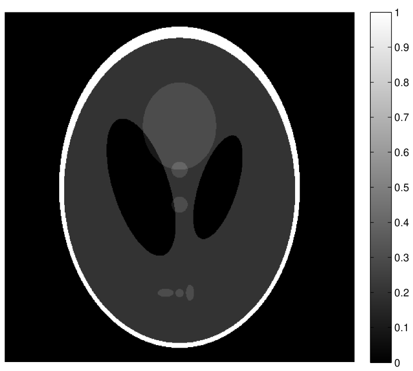
(a) Modified Shepp-Logan

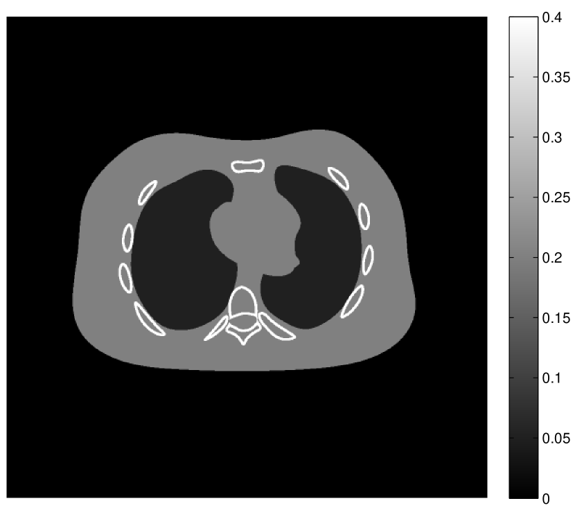
(b) NCAT

(c) Mouse

Figure 1: The datasets used. (c) shows the ground truth converged result from the projections.

We present experiments on two simulated phantoms and one real dataset, see Fig. 1. The phantoms are: the modified 2D Shepp-Logan head phantom [60]; and a 2D slice of the NCAT phantom [61]. The phantoms were generated at a resolution of $512\times 512$ pixels, and ground truth sinograms were generated in ASTRA using a fan beam geometry with $888$ detectors, isotropic pixels of 1 mm, isotropic detectors of $1.0239$ mm, and source-to-detector distance of $949.075$ mm. We assumed Poisson measurement noise with emitted intensity count $I_{0}=10^{5}$ to generate the noisy projections used.

The real dataset is a 2D slice of a 3D cone beam scan of a mouse from the Exxim Cobra software . The data contains 194 projections (over 194 degrees) of a fan beam geometry with 512 detectors of size 0.16176 mm, source-to-detector distance of 529.29 mm, source-to-isocenter distance of 395.73 mm, and reconstructed volume of $512\times 512$ pixels of isotropic size 0.12 mm. We ran 500 iterations of BSSART with $\alpha=0.1$ to generate the ground truth volume, but we note that results on this dataset should be taken with a grain of salt. We measure performance in terms of SNR (signal-to-noise ratio) defined as

$$\mbox{SNR}(x,\hat{x})=10\log\frac{\sum_{j}\hat{x}_{j}^{2}}{\sum_{j}\left(x_{j}-\hat{x}_{j}\right)^{2}}$$

where $x\in\mathbb{R}^{n}$ is the current estimate of the volume and $\hat{x}\in\mathbb{R}^{n}$ is the ground truth volume.

We clip the reconstruction estimate $x$ at the end of each inner iteration (i.e. after each update step) using this function

$$\mbox{clip}(x)=\max(0,x)$$

to get rid of negative voxel values.

We implemented all methods using ASTRA with a mix of C++ and Matlab code. The iterative algorithms not present in ASTRA, namely BICAV, BSSART, and OS-SQS, were implemented in C++. The proximal operators were also implemented in C++. The Linearized ADMM was implemented in Matlab. We also modified existing algorithms in ASTRA to suit our needs e.g. compute SNR, report run times, etc. All experiments were run on one core of an Intel Xeon E5-280 2.7 GHz with 64 GB RAM.

VI-B Iterative Algorithms Comparison

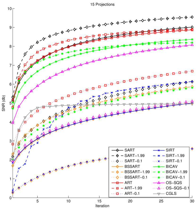
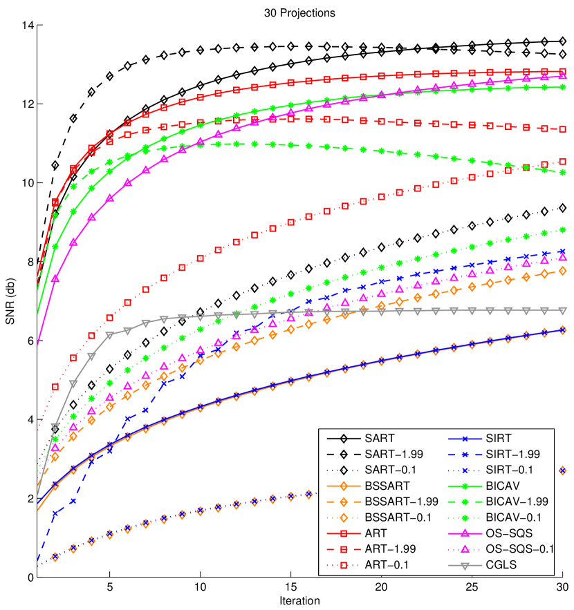
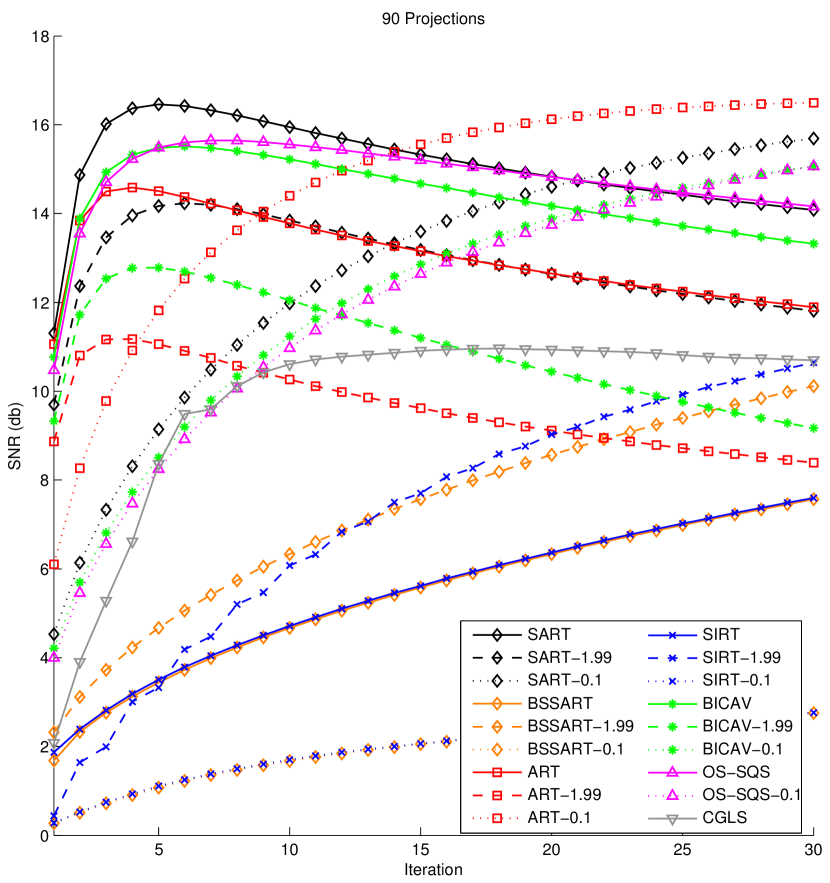
(a) Modified Shepp-Logan

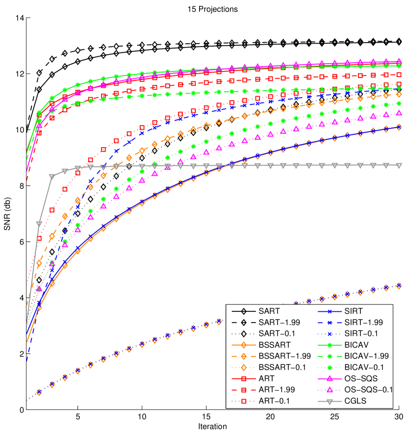
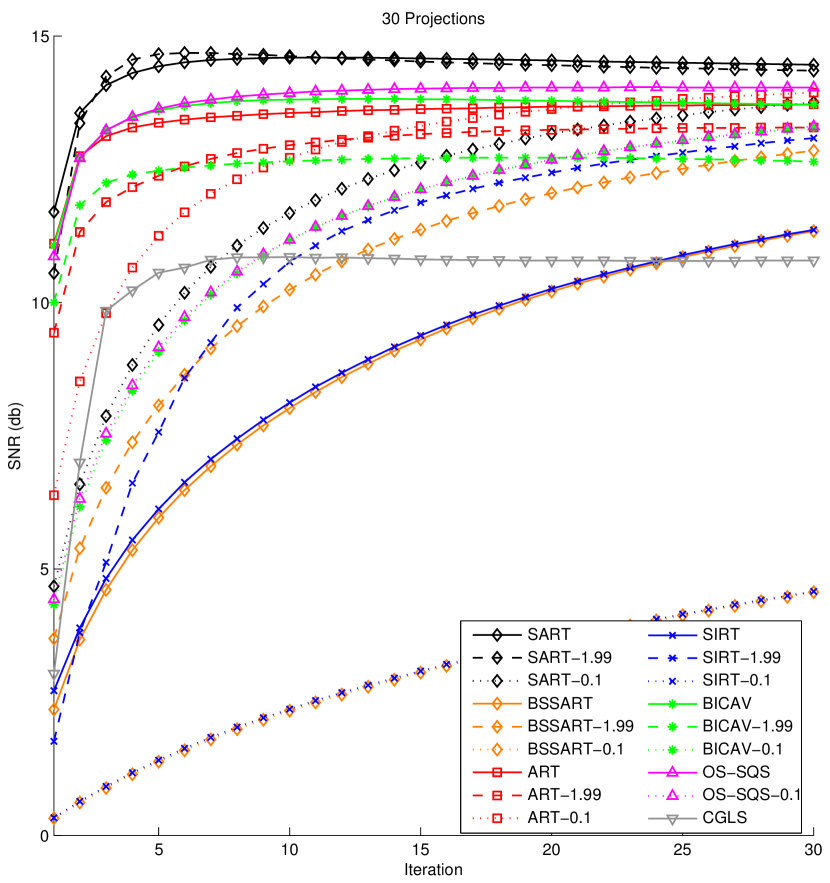
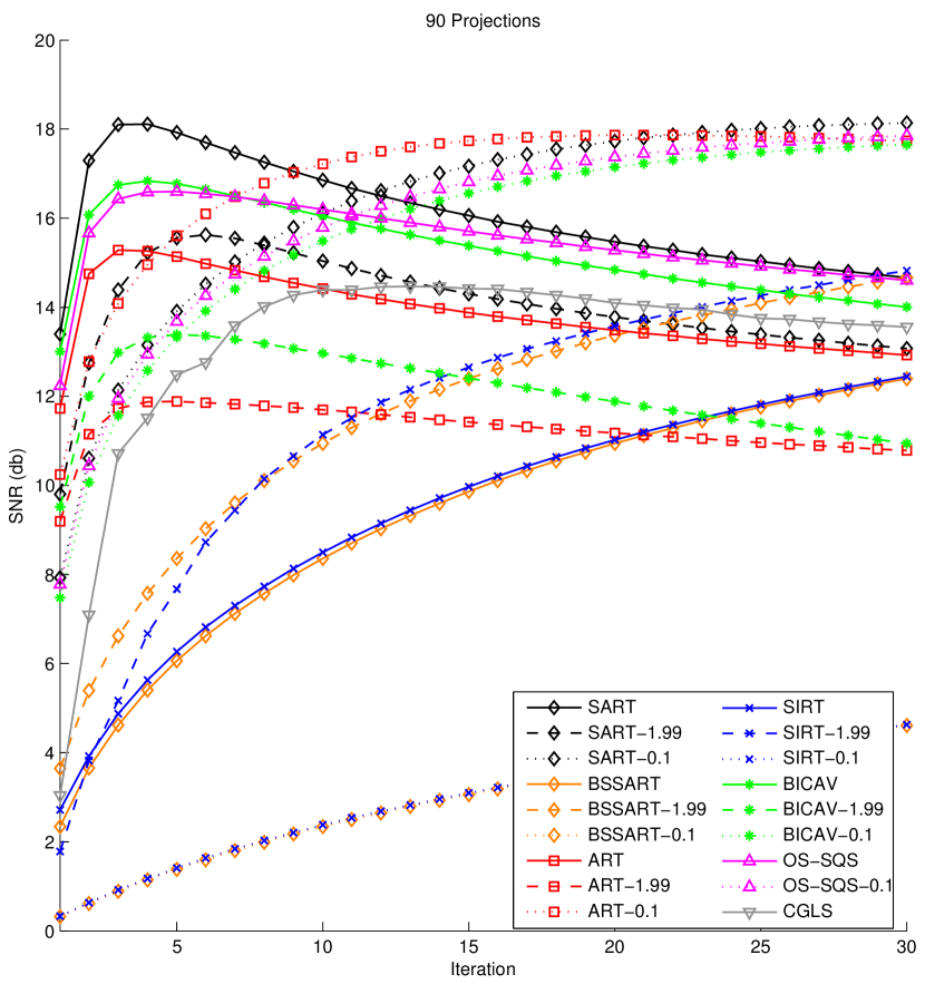
(b) NCAT

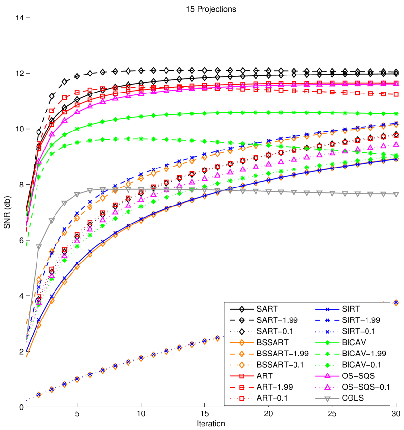
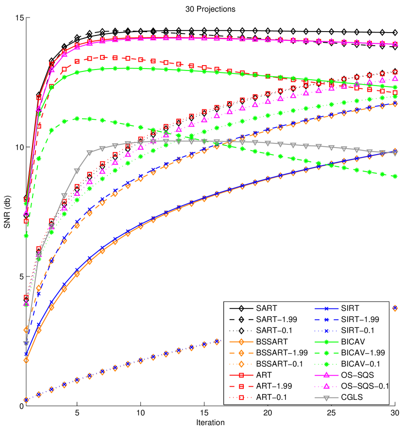
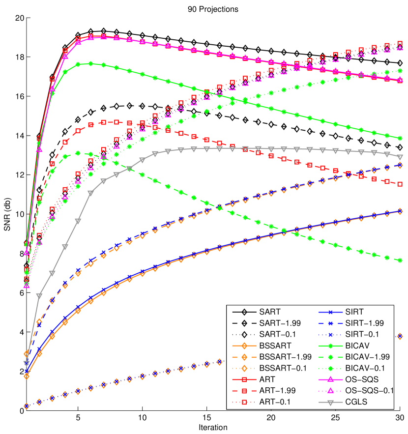
(c) Mouse

Figure 2: Iterative Algorithms Comparison. Plots show SNR per iteration. Solid lines have $\alpha=1$, dashed lines have $\alpha=1.99$, and dotted lines have $\alpha=0.1$.

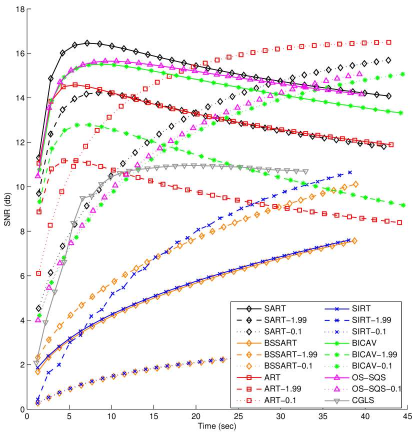
(a) Modified Shepp-Logan

(b) NCAT

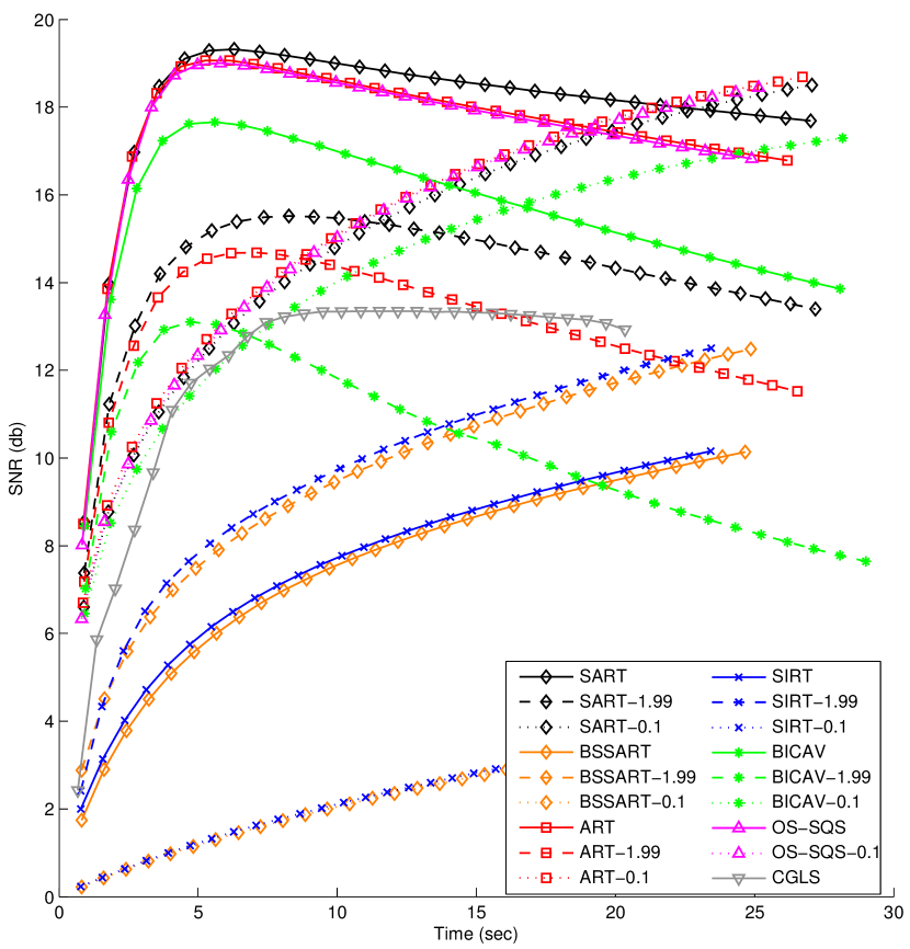
(c) Mouse

Figure 3: Running Time Comparison. Curves show SNR per running time for 90 projections . Compare with Fig. 2 (bottom row).

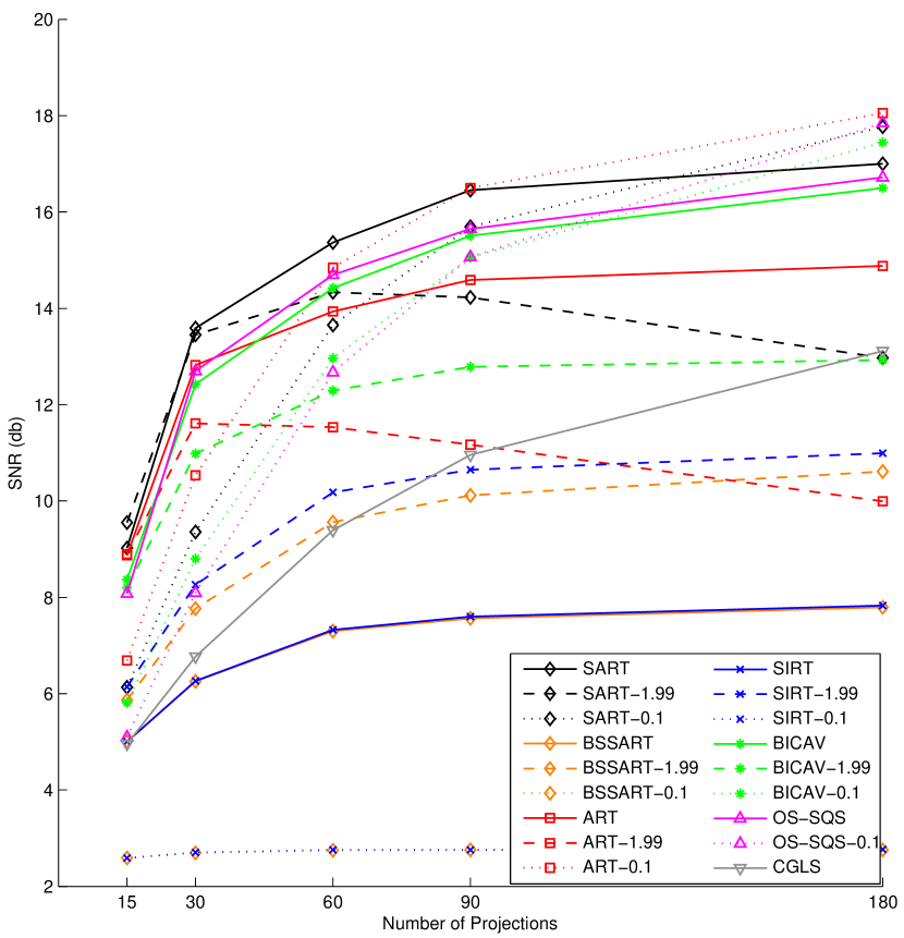
(a) Modified Shepp-Logan

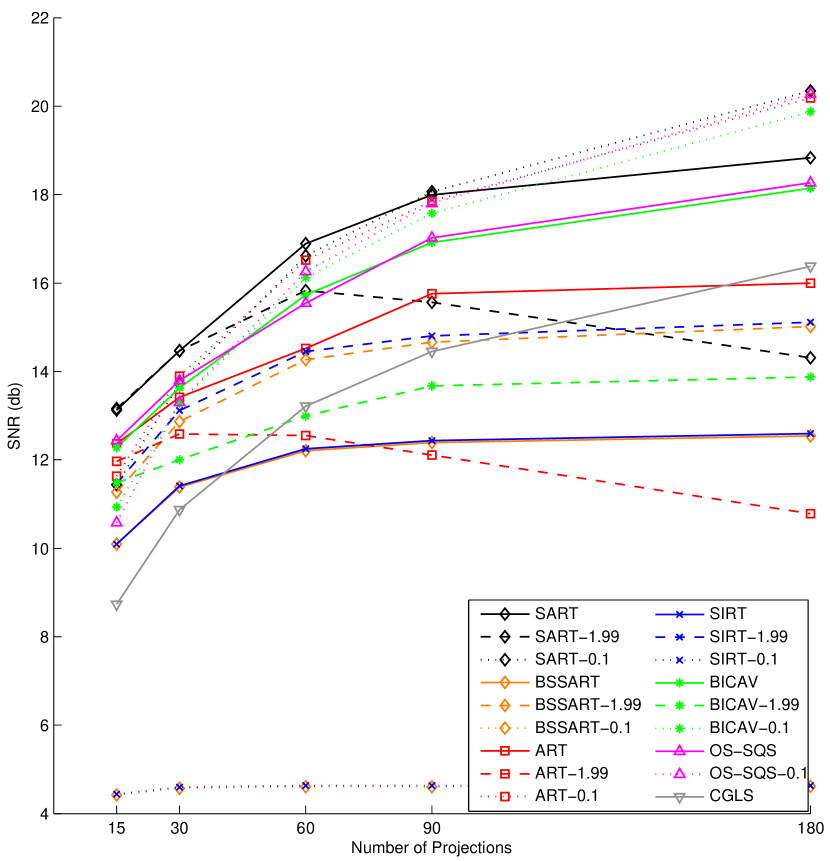
(b) NCAT

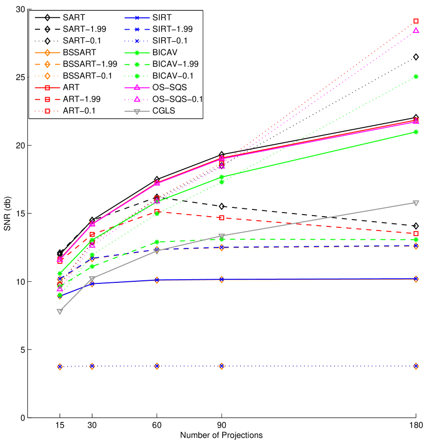
(c) Mouse

Figure 4: Effect of the number of projections. Plots show the maximum SNR achieved over 30 iterations per number of projections used.

We first compare the different iterative algorithms presented in Sec. III on the datasets. We set the number of subsets in OS-SQS to the number of projections to have a fair comparison with SART, since we noticed that increasing the number of subsets increases the convergence rate. We compare different values of $\alpha$, namely 0.1, 1, and 1.99. We compare convergence per iteration since all methods are roughly equal in runtime, as each outer iteration contains (roughly) one forward and one backward projection. This is confirmed in Fig. 3. Note that our implementation is not optimized for any of the methods, and the processing time is just an indication. We initialize all methods with uniform volume $x^{(0)}=\mathbf{0}_{n}$.

Fig. 2 shows the SNR per iteration for 15, 30, 90 projections for 30 iterations. Fig. 4 shows the the maximum SNR over 30 iterations for different number of equally distributed projections from 15 to 180. From the figures, we make the following conclusions:

• The simulated projections closely resemble the results from the real dataset, which suggests that the measurement noise model is reflective of real data.

• With fewer projections (15 or 30 projections), using larger values $\alpha=1.99$ gives faster and better convergence.

• With many projections, moderate values $\alpha=1$ produces a fast convergence that then falls off and is overtaken by $\alpha=0.1$.

• SART provides the fastest convergence within a handful of iterations, and is consistently better for fewer projections. However, it is overtaken by ART and others for many projections. This provides the motivation to use it in the proximal framework, since typically the tomography solver is invoked for only a few iterations per outer iteration of ADMM for example [28].

• With more projections, e.g. 90, we notice that the SNR for a few methods go up and then down. This doesn’t mean, however, that they are not converging. The objective function is the reprojection error not the SNR. This can be explained by the fact of the presence of noise, and that at some point the algorithm starts fitting the noise in the measurements [1]. Usually these kinds of algorithms are run interactively where the user inspects the reconstruction quality every few iterations and stops the procedure when it starts to deteriorate, which motivates Fig. 4.

• Even though BICAV, SIRT, and BSSART have formal proofs of convergence, their convergence speed per iteration is in fact much lower than SART or (this version of) OS-SQS, that lack these proofs.

• The faster convergence and best results are achieved by SART, followed by ART, OS-SQS, and BICAV. They work better with $\alpha=1$ for few projections, and with $\alpha=0.1$ for more projections.

• CGLS, that was used before for solving tomography problems [28, 26], performs quite poorly compared to the other iterative algorithms.

• Using plain iterative methods does not give acceptable results with fewer projections. Thus we focus next on using regularizers in the proximal framework with SART, ART, OS-SQS, and BICAV and fewer projections, namely 30 projections.

VI-C Poisson Model Mapping Functions Comparison

We investigate different mapping functions for the Poisson noise model $f_{\text{P}}(\cdot)$ in Eq. 21 using the ITV regularizer from Eq. 23 using the ADMM algorithm. We compare applying different mapping functions on the weights, since we noticed it improves the performance for some proximal operators. In particular, we try three functions: identity $r_{1}(w_{i})=w_{i}$, the square root $r_{2}=\sqrt{w_{i}}$, and the cubic root $r_{3}=\sqrt[3]{w_{i}}$. Figure 5 shows results for the three datasets for 15 and 30 projections with $\sigma=0.1$ in Eq. 23. We set $\rho=100$ and $\mu=\nicefrac{{1}}{{\rho\|K\|^{2}}}$ except for OS-SQS which was tuned manually as this default value didn’t provide good performance.

We note the following that using mapping $r_{1}$ is generally worse than $r_{2}$ and $r_{3}$. This is especially true for OS-SQS, BICAV, and ART. We believe this is due to the normalizing matrix $C$, where in this case it includes sum of squares of entries in the matrix $A$ that are typically $<1$. This makes them even smaller, and taking the square or cubic root of the weights, which are also $<1$, makes them bigger to counter-balance the former effect, and make the two terms of the optimization problem in Eq. 5 of the same order. This is not the case in SART where the $C$ matrix contains sums of entries of $A$. We also note that ART and SART provide very similar performance, closely followed by BICAV and then OS-SQS. This is also confirmed in the comparison in Sec. VI-E.

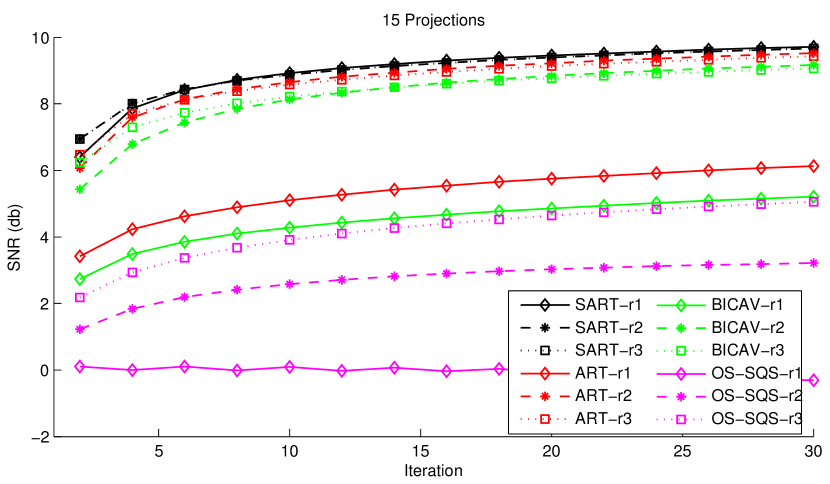
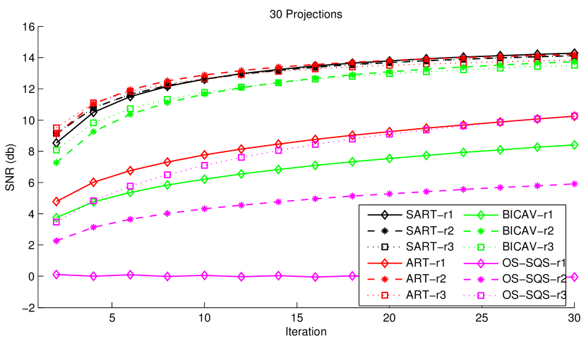
(a) Modified Shepp-Logan

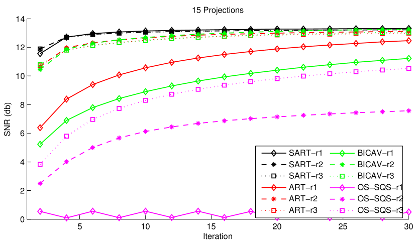
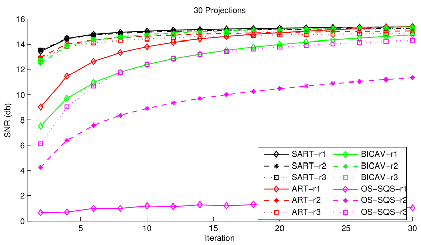
(b) NCAT

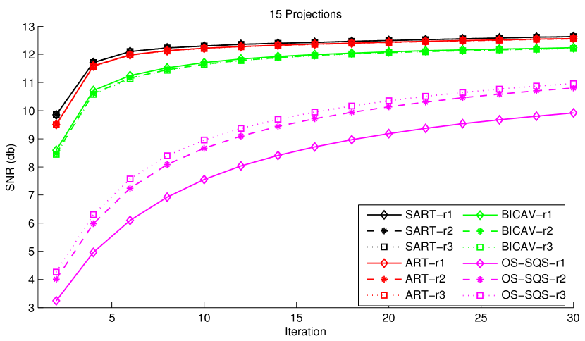
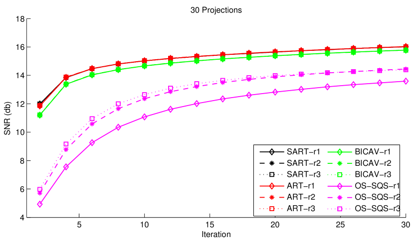
(c) Mouse

Figure 5: TRex Poisson Model Mapping Functions Comparison. Curves show SNR per iteration for the Poisson noise models with mapping functions $r_{1}$ (diamonds), $r_{2}$ (asterisks), and $r_{3}$ (squares). See Sec. VI-C.

VI-D Data Terms and Regularizers Comparison

We compare the different data terms and regularizers defined in Sec. V. We solve the tomography proximal operator (step 3 in Alg. 4) using 2 iterations of the SART proximal operator (from Table II), using $\alpha=1.99$ with for 15 and 30 projections (see Sec. VI-B). We use $\sigma=0.05$ and $\rho=25$ for 15 projections; $\sigma=0.1$ and $\rho=50$ for 30 projections; and set $\mu=\nicefrac{{1}}{{\rho\|K\|^{2}}}$. We initialize all methods with uniform volume $x^{(0)}=\mathbf{0}_{n}$. We estimated the matrix norm $\|K\|$ using the power method. Fig. 6 shows the results for the three datasets, where we plot against the number of SART iterations. We note the following:

• Using the proximal framework provides significantly better results than the unregularized iterative methods in Sec. VI-B. This is expected since adding a powerful regularizer constrains the reconstruction to better resemble the ground truth.

• The Poisson noise model $f_{\text{P}}(\cdot)$ is better than the Gaussian noise model $f_{\text{G}}(\cdot)$ for the datasets, specially with more projections. This is consistent with the noise model used to generate the noisy simulated sinograms, and with the physical noise model in the real dataset.

• With more projections, more regularization (higher $\sigma$) produces better results while for fewer projections less regularization is sufficient . This is expected because using more projections adds more constraints (rows in the projection matrix $A$) that need better regularization to get good results.

• The SAD regularizer is better for all datasets.

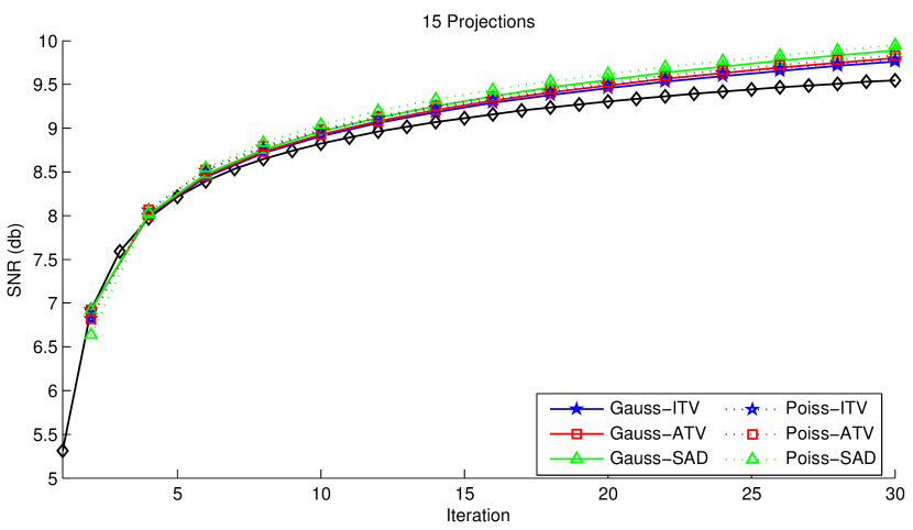
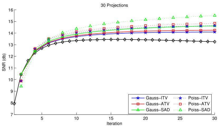
(a) Modified Shepp-Logan

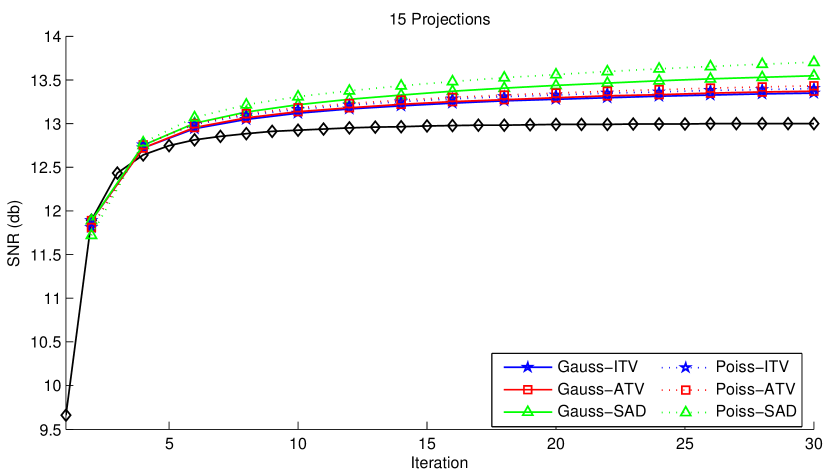
(b) NCAT

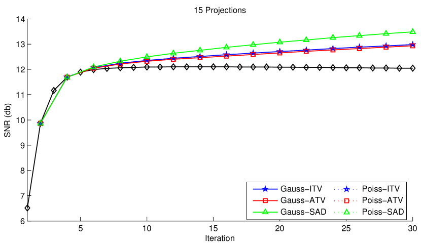
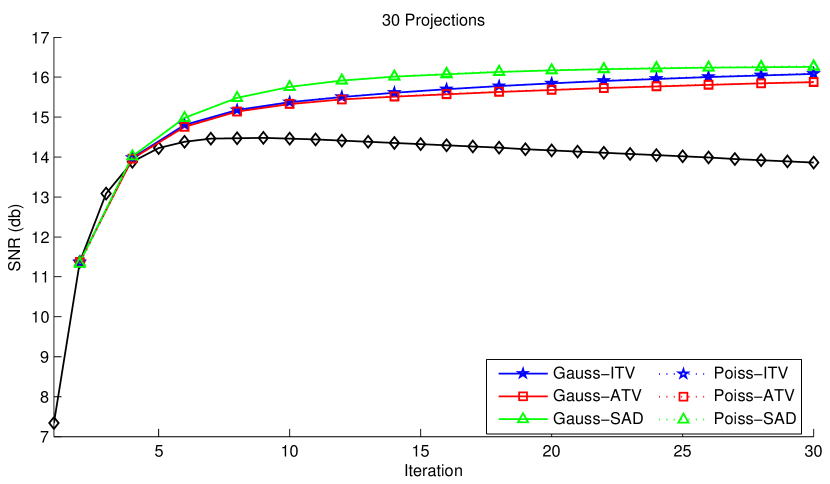
(c) Mouse

Figure 6: Data Terms and Regularizers Comparison. Plots show SNR per iteration for the Gaussian (solid curves) and Poisson (dashed curves)noise models with ITV (blue), ATV (red), and SAD (green) regularizers. The black curve shows the results for SART. See Sec. VI-D.

VI-E Proximal Operators Comparison

We compare the different proximal operators from Sec. IV (SART, ART, OS-SQS, and BICAV) and Table II using our proximal framework in Alg. 4. We use the best regularizer from Sec. VI-D, i.e. SAD regularizer, and both the Poisson and Gaussian noise models. For the Poisson model, we use $r_{1}$ mapping for SART, and $r_{3}$ for ART, BICAV, and OS-SQS since $r_{1}$ does produce good results (see Sec. VI-C). We set $\sigma=0.05$ and $\rho=50$ for 15 projections; and $\sigma=0.1$ and $\rho=100$ for 30 projections. We set $\mu=\nicefrac{{1}}{{\rho\|K\|^{2}}}$ except for OS-SQS which had to be tuned manually. We note the following:

• The Poisson model is consistently better than the Gaussian model for all operators and all datasets.

• SART proximal operator is generally better than other proximal operators, and ART and BICAV are quite competitive.

• OS-SQS provides the worst performance. We think this has to do with structure of the update formula in Table II, where the gradient update $A_{S}^{T}(p_{S}-A_{S}x^{(t)})$ is added to the difference between the current estimate and the input to the proximal operator $u-x^{(t)}$, where the scaling between the two terms has to be adjusted properly. That is the reason $\mu$ had to be carefully tuned to get better results.

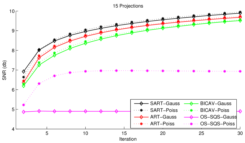
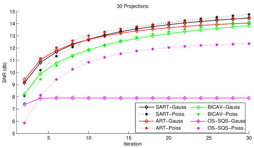
(a) Modified Shepp-Logan

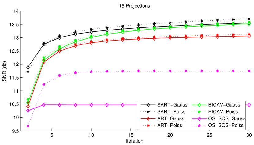
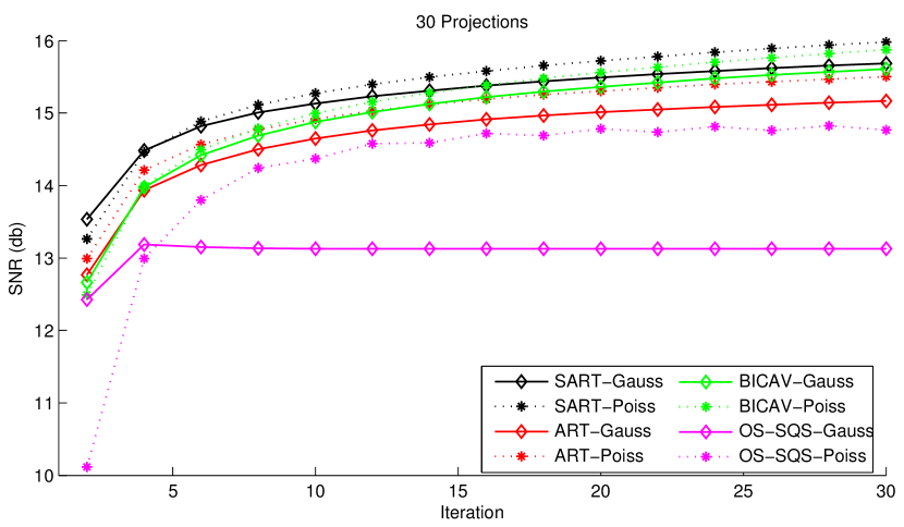
(b) NCAT

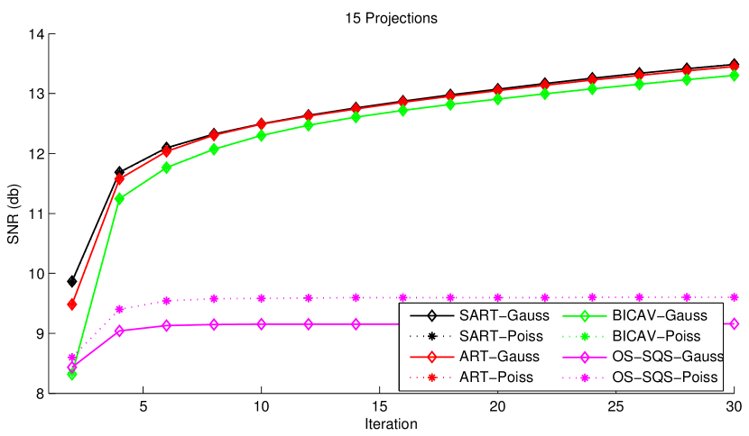
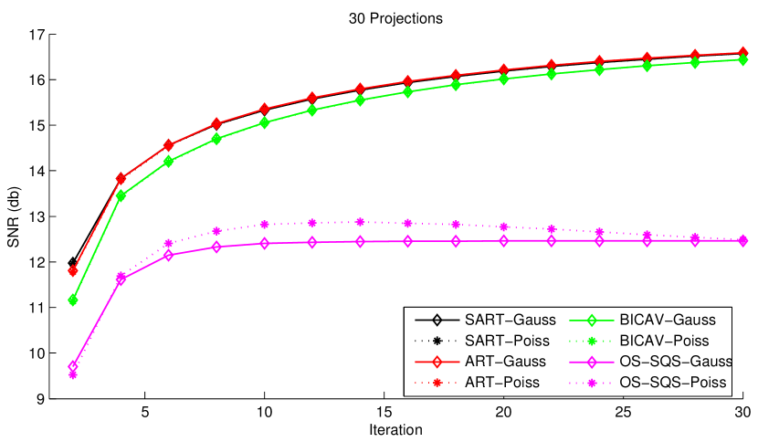
(c) Mouse

Figure 7: TRex Proximal Operators Comparison. Plots show SNR per iteration for the Gaussian (solid curves) and Poisson (dashed curves) noise models with SAD regularizer. See Sec. VI-E.

VI-F Comparison to State of the Art

We compare our framework to two state of the art methods: the ADMM-PCG method of Ramani et al. [28] and the OS-MOM method from Kim et al. [29] that combines ordered subsets with momentum. We don’t compare to the method of Nien et al. [21] because the authors indicate that the performance is closely matched by the OS-MOM method and is quite similar.

The ADMM-PCG minimizes a combination of a WLS data term and regularization term

$$\min_{x}\frac{1}{2}\|p-Ax\|_{W}^{2}+\lambda\sum_{r=1}^{n}\kappa_{r}\|Rx_{r}\|_{1}$$

where $\kappa_{r}\in\mathbb{R}$ are spatial weights that govern the spatial resolution in the reconstruction and $Rx_{r}\in\mathbb{R}^{d}$ is the vector of wavelet decomposition at voxel $x_{r}$. It uses 2 iterations of PCG to solve the proximal operator of the data term, as opposed to our framework that uses SART, ART, … etc. We run the Matlab code available online from the author as part of the IRT toolbox. The default procedure for choosing the parameters didn’t work well with our datasets, so we had to manually tweak the parameters, [28]. We set $\nu=2\times 10^{5}$, $\lambda=10^{-3}$, and $\mu=10^{-4}$ for 15 projections and $\mu=10^{-3}$ for 30 projections. We use the Wavelet decomposition basis with the $\ell_{1}$ norm regularizer.

The OS-Mom also minimizes a WLS data term and regularization term

$$\min_{x}\frac{1}{2}\|p-Ax\|_{W}^{2}+\beta\sum_{r=1}^{n}\psi(\nabla x_{r})$$

where $\psi(\cdot)$ is an edge preserving potential function and $\nabla x_{r}\in\mathbb{R}^{2}$ is the gradient at voxel $x_{r}$. We implemented the Momentum 2 method (Table IV in [29]) within the IRT toolbox. We use the settings from the paper for the regularizer i.e. the Fair potential

$$\psi(t)=\frac{\delta^{2}}{b^{3}}\left(\frac{ab^{2}}{2}\left|\frac{t}{\delta}\right|^{2}+b(b-a)\left|\frac{t}{\delta}\right|+(a-b)\log(1+b\left|\frac{t}{\delta}\right|)\right)$$

with $\delta=10$, $a=0.0558$, and $b=1.6395$, and bit reversal for subset ordering. We tweaked $\beta$ and $M$ [29] to get good performance. We set $\beta=0.05$ and $M=5$ subsets for 15 projections and $\beta=0.1$ and $M=10$ subsets for 30 projections. We use relaxation with parameter $10^{-3}$ to help the convergence. We also compare to plain OS method without momentum with the same WLS data term and regularizer as OS-Mom.

Fig. 8 shows a comparison with these two algorithm. The TRex uses the SART proximal operator with Poisson noise model and $r_{1}$ mapping and SAD regularizer. We set $\sigma=0.05$ and $\rho=25$ for 15 projections and $\sigma=0.1$ and $\rho=50$ for 30 projections, and set $\mu=\nicefrac{{1}}{{\rho\|K\|^{2}}}$. We initialize all methods with a uniform volume $x^{(0)}=\mathbf{0}_{n}$. Fig. 9 shows sample reconstruction results for 30 projections after 30 iterations. We note the following:

• The ADMM-PCG method’s performance is quite bad with these datasets. They require a lot of tweaking to get them to work correctly since the automated estimation methods described in [28] didn’t work. Moreover, the method seems very sensitive to the values of the parameters, and thus is harder to tweak.

• The OS-Mom method indeed accelerates the convergence of the OS method at early iterations [29]. However, its performance is not consistent across datasets, where some times it is good and most of the time the SNR starts decreasing after a while, even with relaxation.

• TRex with SART and SAD consistently performs better and ends up with higher SNR than ADMM-PCG or OS-Mom. Moreover, it is easier to tweak and not very sensitive to the choice of parameters. Note that for NCAT and Mouse, using TRex, we get SNR with 15 projections that equals the SNR we get with 30 projections using plain SART.

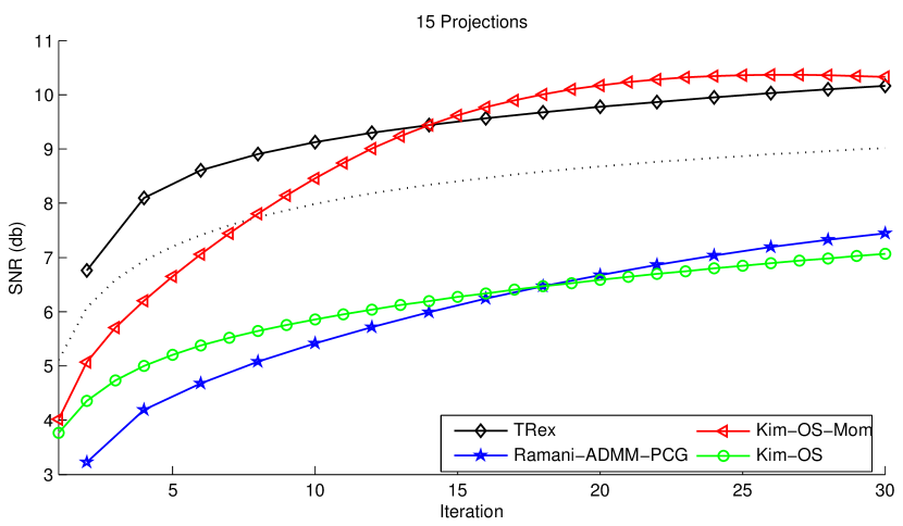
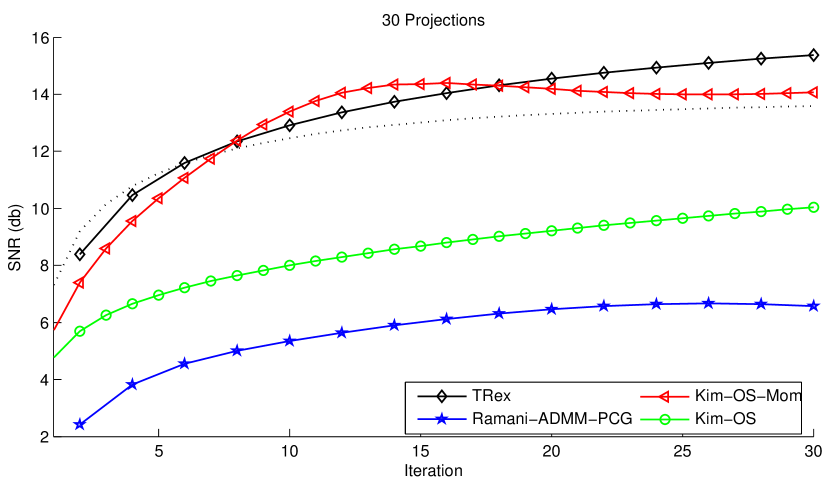
(a) Modified Shepp-Logan

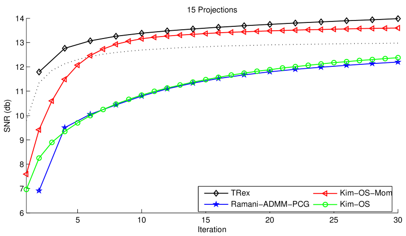
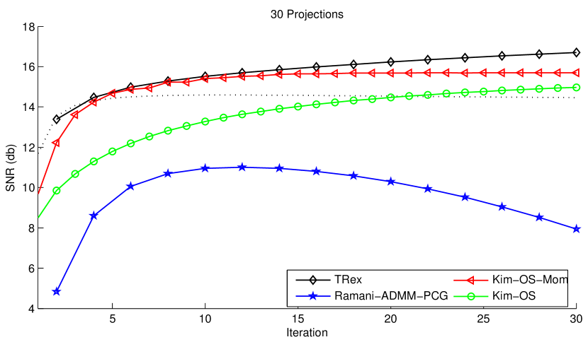
(b) NCAT

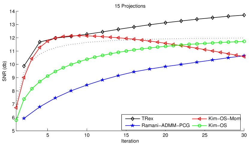
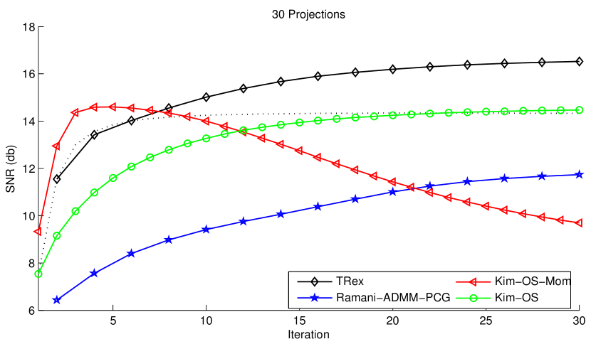
(c) Mouse

Figure 8: TRex Comparison to Sate of the Art. Plots show SNR per iteration. The TRex framework uses SART with Poisson model and SAD regularizer. The dotted curve shows the baseline plain SART (from Sec. VI-B). See Sec. VI-F.

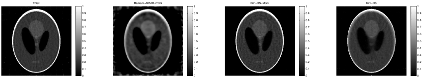
(a) Modified Shepp-Logan

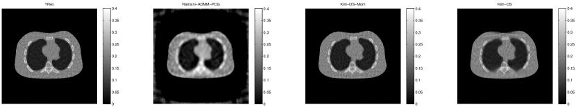
(b) NCAT

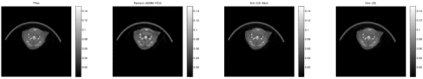
(c) Mouse

Figure 9: TRex Comparison to Sate of the Art. Reconstruction results for 30 projections after 30 iterations. TRex uses SART with Poisson model and SAD regularizer. See Sec. VI-F.

VII Conclusions

We presented TRex, a flexible proximal framework for robust tomography reconstruction in sparse view applications. TRex relies on using iterative methods, e.g. SART, for directly solving the tomography proximal operator. We first compare the famous tomography iterative solvers, and then derive proximal operators for the best four methods. We then show how to use TRex to solve using different noise models (Gaussian and Poisson) and using different powerful regularizers (ITV, ATV, and SAD). We show that TRex outperforms state of the art methods, namely ADMM-PCG [28] and OS-Mom [29], and is easy to tune. We conclude that SART—even though is not guaranteed to converge—offers the best tomography solver for sparse view applications, followed closely by ART and BICAV.

We plan to extend this work in several ways: (a) study how to incorporate momentum acceleration into SART as in [29]; (b) study how to use preconditioners with SART such as the Fourier-based cone filter preconditioners [44]; (c) study other applications such as low-dosage X-ray tomography, which changes the nature of the measurement noise [62]; and (d) implement and apply TRex to 3D cone beam reconstruction and compare to other famous packages such as RTK [40].

References

- [1] G. T. Herman, Fundamentals of computerized tomography: image reconstruction from projections. Springer Science & Business Media, 2009.
- [2] J.-B. Thibault, K. D. Sauer, C. A. Bouman, and J. Hsieh, “A three-dimensional statistical approach to improved image quality for multislice helical ct,” Medical physics, vol. 34, no. 11, pp. 4526–4544, 2007.
- [3] R. Zhang, J.-B. Thibault, C. A. Bouman, K. D. Sauer, and J. Hsieh, “Model-based iterative reconstruction for dual-energy x-ray ct using a joint quadratic likelihood model,” Medical Imaging, IEEE Transactions on, vol. 33, no. 1, pp. 117–134, 2014.
- [4] A. C. Kak and M. Slaney, Principles of computerized tomographic imaging. Society for Industrial and Applied Mathematics, 2001.
- [5] R. Gordon, R. Bender, and G. T. Herman, “Algebraic reconstruction techniques (art) for three-dimensional electron microscopy and x-ray photography,” Journal of theoretical Biology, vol. 29, no. 3, pp. 471–481, 1970.
- [6] R. Gordon and G. T. Herman, “Reconstruction of pictures from their projections,” Communications of the ACM, vol. 14, no. 12, pp. 759–768, 1971.
- [7] G. Ramachandran and A. Lakshminarayanan, “Three-dimensional reconstruction from radiographs and electron micrographs: application of convolutions instead of fourier transforms,” PNAS, vol. 68, no. 9, pp. 2236–2240, 1971.
- [8] L. A. Shepp and B. F. Logan, “The fourier reconstruction of a head section,” Nuclear Science, IEEE Transactions on, vol. 21, no. 3, pp. 21–43, 1974.
- [9] L. Feldkamp, L. Davis, and J. Kress, “Practical cone-beam algorithm,” Journal of the Optical Society of America, vol. 1, no. 6, pp. 612–619, 1984.
- [10] X. Pan, E. Y. Sidky, and M. Vannier, “Why do commercial ct scanners still employ traditional, filtered back-projection for image reconstruction?,” Inverse problems, vol. 25, no. 12, p. 123009, 2009.
- [11] A. Andersen and A. C. Kak, “Simultaneous algebraic reconstruction technique (sart): a superior implementation of the art algorithm,” Ultrasonic imaging, vol. 6, no. 1, pp. 81–94, 1984.
- [12] A. H. Andersen, “Algebraic reconstruction in ct from limited views,” Medical Imaging, IEEE Transactions on, vol. 8, no. 1, pp. 50–55, 1989.
- [13] P. Gilbert, “Iterative methods for the reconstruction of three-dimensional objects from projections,” J. theor. Biol, vol. 36, no. 105, pp. 117–127, 1972.
- [14] Y. Censor and T. Elfving, “Block-iterative algorithms with diagonally scaled oblique projections for the linear feasibility problem,” SIAM Journal on Matrix Analysis and Applications, vol. 24, no. 1, pp. 40–58, 2002.
- [15] Y. Censor, D. Gordon, and R. Gordon, “Bicav: A block-iterative parallel algorithm for sparse systems with pixel-related weighting,” Medical Imaging, IEEE Transactions on, vol. 20, no. 10, pp. 1050–1060, 2001.
- [16] A. Björck, Numerical methods for least squares problems. Siam, 1996.
- [17] A. R. De Pierro, “A modified expectation maximization algorithm for penalized likelihood estimation in emission tomography.,” IEEE Transactions on Medical Imaging, vol. 14, no. 1, pp. 132–137, 1994.
- [18] H. M. Hudson and R. S. Larkin, “Accelerated image reconstruction using ordered subsets of projection data,” Medical Imaging, IEEE Transactions on, vol. 13, no. 4, pp. 601–609, 1994.
- [19] H. Erdogan and J. A. Fessler, “Ordered subsets algorithms for transmission tomography,” Physics in medicine and biology, vol. 44, no. 11, p. 2835, 1999.
- [20] D. Kim, D. Pal, J.-B. Thibault, and J. A. Fessler, “Accelerating ordered subsets image reconstruction for x-ray ct using spatially nonuniform optimization transfer,” Medical Imaging, IEEE Transactions on, vol. 32, no. 11, pp. 1965–1978, 2013.
- [21] H. Nien and J. Fessler, “Fast x-ray ct image reconstruction using a linearized augmented lagrangian method with ordered subsets,” Medical Imaging, IEEE Transactions on, vol. 34, pp. 388–399, Feb 2015.
- [22] S. Boyd, N. Parikh, E. Chu, B. Peleato, and J. Eckstein, “Distributed optimization and statistical learning via the alternating direction method of multipliers,” Foundations and Trends® in Machine Learning, vol. 3, no. 1, pp. 1–122, 2011.
- [23] N. Parikh and S. Boyd, “Proximal algorithms,” Foundations and Trends in Optimization, vol. 1, no. 3, pp. 123–231, 2013.
- [24] N. H. Clinthorne, T.-S. Pan, P.-C. Chiao, W. Rogers, and J. Stamos, “Preconditioning methods for improved convergence rates in iterative reconstructions,” Medical Imaging, IEEE Transactions on, vol. 12, no. 1, pp. 78–83, 1993.
- [25] L. I. Rudin, S. Osher, and E. Fatemi, “Nonlinear total variation based noise removal algorithms,” Physica D: Nonlinear Phenomena, vol. 60, no. 1, pp. 259–268, 1992.
- [26] E. Y. Sidky, J. H. Jørgensen, and X. Pan, “Convex optimization problem prototyping for image reconstruction in computed tomography with the chambolle–pock algorithm,” Physics in medicine and biology, vol. 57, no. 10, p. 3065, 2012.
- [27] J. Gregson, M. Krimerman, M. B. Hullin, and W. Heidrich, “Stochastic tomography and its applications in 3d imaging of mixing fluids,” ACM Trans. Graph. (Proc. SIGGRAPH 2012), vol. 31, no. 4, pp. 52:1–52:10, 2012.
- [28] S. Ramani and J. A. Fessler, “A splitting-based iterative algorithm for accelerated statistical x-ray ct reconstruction,” Medical Imaging, IEEE Transactions on, vol. 31, no. 3, pp. 677–688, 2012.
- [29] D. Kim, S. Ramani, and J. A. Fessler, “Combining ordered subsets and momentum for accelerated x-ray ct image reconstruction,” Medical Imaging, IEEE Transactions on, vol. 34, no. 1, pp. 167–178, 2015.
- [30] M. Aly, G. Zang, W. Heidrich, and P. Won, “A tomography reconstruction proximal framework for robust sparse view x-ray applications,” arXiv preprint arXiv:xyz.
- [31] W. van Aarle, W. J. Palenstijn, J. De Beenhouwer, T. Altantzis, S. Bals, K. J. Batenburg, and J. Sijbers, “The astra toolbox: A platform for advanced algorithm development in electron tomography,” Ultramicroscopy, vol. 157, pp. 35–47, 2015.
- [32] A. Lent, “A convergent algorithm for maximum entropy image restoration, with a medical x-ray application,” Image Analysis and Evaluation, pp. 249–257, 1977.
- [33] L. A. Shepp and Y. Vardi, “Maximum likelihood reconstruction for emission tomography,” Medical Imaging, IEEE Transactions on, vol. 1, no. 2, pp. 113–122, 1982.
- [34] Y. Censor, “Finite series-expansion reconstruction methods,” Proceedings of the IEEE, vol. 71, no. 3, pp. 409–419, 1983.
- [35] S. Kaczmarz, “Angenäherte auflösung von systemen linearer gleichungen,” Bulletin International de l’Academie Polonaise des Sciences et des Lettres, vol. 35, pp. 355–357, 1937.
- [36] J. Gregor and J. A. Fessler, “Comparison of sirt and sqs for regularized weighted least squares image reconstruction,” Computational Imaging, IEEE Transactions on, vol. 1, no. 1, pp. 44–55, 2015.
- [37] I. A. Elbakri and J. A. Fessler, “Statistical image reconstruction for polyenergetic x-ray computed tomography,” Medical Imaging, IEEE Transactions on, vol. 21, no. 2, pp. 89–99, 2002.
- [38] J. Wang, T. Li, H. Lu, and Z. Liang, “Penalized weighted least-squares approach to sinogram noise reduction and image reconstruction for low-dose x-ray computed tomography,” Medical Imaging, IEEE Transactions on, vol. 25, no. 10, pp. 1272–1283, 2006.
- [39] E. Y. Sidky and X. Pan, “Image reconstruction in circular cone-beam computed tomography by constrained, total-variation minimization,” Physics in medicine and biology, vol. 53, no. 17, p. 4777, 2008.
- [40] C. Mory, B. Zhang, V. Auvray, M. Grass, D. Schafer, F. Peyrin, S. Rit, P. Douek, and L. Boussel, “Ecg-gated c-arm computed tomography using l1 regularization,” in Signal Processing Conference (EUSIPCO), 2012 Proceedings of the 20th European, pp. 2728–2732, IEEE, 2012.
- [41] H. H. Bauschke and P. L. Combettes, Convex analysis and monotone operator theory in Hilbert spaces. Springer Science & Business Media, 2011.
- [42] P. L. Combettes and J.-C. Pesquet, “Proximal splitting methods in signal processing,” in Fixed-point algorithms for inverse problems in science and engineering, pp. 185–212, Springer, 2011.
- [43] A. Chambolle and T. Pock, “A first-order primal-dual algorithm for convex problems with applications to imaging,” Journal of Mathematical Imaging and Vision, vol. 40, no. 1, pp. 120–145, 2011.
- [44] J. A. Fessler and S. D. Booth, “Conjugate-gradient preconditioning methods for shift-variant pet image reconstruction,” Image Processing, IEEE Transactions on, vol. 8, no. 5, pp. 688–699, 1999.
- [45] E. Esser, X. Zhang, and T. F. Chan, “A general framework for a class of first order primal-dual algorithms for convex optimization in imaging science,” SIAM Journal on Imaging Sciences, vol. 3, no. 4, pp. 1015–1046, 2010.
- [46] A. Beck and M. Teboulle, “A fast iterative shrinkage-thresholding algorithm for linear inverse problems,” SIAM Journal on Imaging Sciences, vol. 2, no. 1, pp. 183–202, 2009.
- [47] J. Klukowska, R. Davidi, and G. T. Herman, “Snark09–a software package for reconstruction of 2d images from 1d projections,” Computer methods and programs in biomedicine, vol. 110, no. 3, pp. 424–440, 2013.
- [48] S. Rit, M. V. Oliva, S. Brousmiche, R. Labarbe, D. Sarrut, and G. C. Sharp, “The reconstruction toolkit (rtk), an open-source cone-beam ct reconstruction toolkit based on the insight toolkit (itk),” in Journal of Physics: Conference Series, vol. 489, p. 012079, IOP Publishing, 2014.
- [49] K. Tanabe, “Projection method for solving a singular system of linear equations and its applications,” Numerische Mathematik, vol. 17, no. 3, pp. 203–214, 1971.
- [50] M. Jiang and G. Wang, “Convergence of the simultaneous algebraic reconstruction technique (sart),” Image Processing, IEEE Transactions on, vol. 12, no. 8, pp. 957–961, 2003.
- [51] K. Mueller and R. Yagel, “Rapid 3-d cone-beam reconstruction with the simultaneous algebraic reconstruction technique (sart) using 2-d texture mapping hardware,” Medical Imaging, IEEE Transactions on, vol. 19, no. 12, pp. 1227–1237, 2000.
- [52] K. Mueller, R. Yagel, and J. J. Wheller, “Fast implementations of algebraic methods for three-dimensional reconstruction from cone-beam data,” Medical Imaging, IEEE Transactions on, vol. 18, no. 6, pp. 538–548, 1999.
- [53] S. Ahn and J. A. Fessler, “Globally convergent image reconstruction for emission tomography using relaxed ordered subsets algorithms,” Medical Imaging, IEEE Transactions on, vol. 22, no. 5, pp. 613–626, 2003.
- [54] X. Zhang, M. Burger, and S. Osher, “A unified primal-dual algorithm framework based on bregman iteration,” Journal of Scientific Computing, vol. 46, no. 1, pp. 20–46, 2011.
- [55] J. Eckstein, “Some saddle-function splitting methods for convex programming,” Optimization Methods and Software, vol. 4, no. 1, pp. 75–83, 1994.
- [56] M. Fazel, T. K. Pong, D. Sun, and P. Tseng, “Hankel matrix rank minimization with applications to system identification and realization,” SIAM Journal on Matrix Analysis and Applications, vol. 34, no. 3, pp. 946–977, 2013.
- [57] C. Chen, R. H. Chan, S. Ma, and J. Yang, “Inertial proximal admm for linearly constrained separable convex optimization,” SIAM Journal on Imaging Sciences, vol. 8, no. 4, pp. 2239–2267, 2015.
- [58] G. Yuan and B. Ghanem, “l0tv: A new method for image restoration in the presence of impulse noise,” in CVPR, vol. 23, pp. 2448–2478, 2015.
- [59] J. Hsieh, Computed Tomography: Principles, Design, Artifacts, and Recent Advances. SPIE Press, 2009.
- [60] P. A. Toft and J. A. Sørensen, The Radon transform-theory and implementation. PhD thesis, Technical University of DenmarkDanmarks Tekniske Universitet, Department of Informatics and Mathematical ModelingInstitut for Informatik og Matematisk Modellering, 1996.
- [61] W. P. Segars and B. M. Tsui, “Study of the efficacy of respiratory gating in myocardial spect using the new 4-d ncat phantom,” Nuclear Science, IEEE Transactions on, vol. 49, no. 3, pp. 675–679, 2002.
- [62] J. Xu and B. M. Tsui, “Quantifying the importance of the statistical assumption in statistical x-ray ct image reconstruction,” Medical Imaging, IEEE Transactions on, vol. 33, no. 1, pp. 61–73, 2014.