Robust integral formulations for electromagnetic scattering from three-dimensional cavities

Abstract

Scattering from large, open cavity structures is of importance in a variety of electromagnetic applications. In this paper, we propose a new well conditioned integral equation for scattering from general open cavities embedded in an infinite, perfectly conducting half-space. The integral representation permits the stable evaluation of both the electric and magnetic field, even in the low-frequency regime, using the continuity equation in a post-processing step. We establish existence and uniqueness results, and demonstrate the performance of the scheme in the cavity-of-revolution case. High-order accuracy is obtained using a Nyström discretization with generalized Gaussian quadratures.

1 Introduction

The computation of electromagnetic wave propagation in the presence of large, open cavities is an important modeling task. It is critical, for example, in understanding the effect of exhaust nozzles and engine inlets on aircraft, as well as surface deformations in automobiles and other land-based vehicles [GW1, GJP, PLA15, JIN2, JL2014]. The presence of such structures plays a dominant role in both the near field, where electromagnetic interference is of concern, and in the far field, where the radar cross-section can be used for identification and classification (including stealth-related calculations). Fast and accurate solvers to simulate such scattering phenomena are essential for both design optimization and verification.

A variety of numerical methods have been proposed to solve such scattering problems. Largely speaking, they fall into two categories. The first is direct numerical simulation using finite difference [GW1], finite element [JIN2], mode-matching [GLin] and boundary integral methods [GW1, Perez-Arancibia2014]. The second is asymptotic methods, including Gaussian beam approximations [GBS] and physical optics-based schemes [SHT]. The latter methods tend to work well at very high frequencies in the absence of multiple near-field scattering events, and are generally not well suited for high-precision calculations in geometrically complex environments. Solving the governing Maxwell equations using finite difference and finite element methods, on the other hand, requires the discretization of an unbounded domain. In practice, these methods must either employ approximate outgoing boundary conditions to mimic the radiation condition at infinity, or be coupled with a boundary integral representation beyond some distance so that the radiation condition is satisfied exactly. In the present work, we will focus on boundary integral equation methods since they are free from grid-based numerical dispersion, can achieve high-order accuracy in complex geometry, and require degrees of freedom only on the boundary of the scatterer itself, greatly reducing the number of unknowns. The Green’s function used to represent the solution satisfies the outgoing (radiation) condition exactly. Existing integral representations for cavity problems, however, generally yield integral equations of the first-kind [HGA2]. First-kind equations can lead to ill-conditioned discrete linear systems, especially if substantial mesh refinement is required. Refined meshes may be needed, for example, to resolve geometric singularities. Furthermore, several existing formulations also suffer from spurious resonances, including those of mixed first-/second-kind systems [Perez-Arancibia2014]. Finally, because of the nature of the dyadic Green’s function for the electric field, standard methods based on discretizing the physical electric current also suffer from low-frequency breakdown [EG10, ZC2000]. This behavior is discussed in more detail below.

In this paper, we propose a new representation of the scattered field that leads to a well-posed (resonance-free) integral equation which is immune from low-frequency breakdown. This allows for a stable numerical discretization along arbitrarily adaptive meshes. In our numerical examples, using the the fact that the scatterer (i.e. the cavity) is axisymmetric permits us to use separation of variables in cylindrical coordinates, applying the Fourier transform in the angular (azimuthal) variable. This procedure leads to a sequence of uncoupled two-dimensional boundary integral equations on the generating curve that defines the cross-section of the boundary of the scatterer (see Fig. 3). There are various numerical technicalities associated with implementing body-of-revolution integral equation solvers, and we do not seek to review the substantial literature here. We instead refer the reader to [HK2014, Kucharski2000, Hao2015, YHM2012, Liu2015] and the references therein. A concise overview of the discretization and resulting solver is given in Section 5. Similar high-order techniques have been applied to solve the Helmholtz equation on surfaces of revolution [HK2014, Hao2015, YHM2012, Liu2015] and the full Maxwell equations (for closed-cavity resonance problems) in [HK15].

Due to the applicability of cavity scattering in physics and engineering, there has been much work dedicated to both the mathematical and numerical aspects of the problem. The well-posedness of the (forward) scattering problem is discussed in [HGA1, HGA2] in the case of the two-dimensional problem, and in [HGA3] for the three-dimensional case. The paper [GKZ] provides the explicit dependence of the scattered field on the wavenumber in the high-frequency context. In [GJP, Li2012], the authors studied uniqueness and stability issues for the inverse problem, where one seeks to recover the shape of an unknown cavity using near-field data. The corresponding optimal design problem, i.e. to find a cavity shape that minimizes the radar cross section, under certain constraints, is discussed in [BJL1, BJL2] in the two-dimensional setting.

An outline of the paper follows: Section 2 provides a detailed introduction to the problem of scattering from an open cavity and proposes an integral representation that leads to a well conditioned integral formulation. In Section 3, we prove that this integral equation has a unique solution for a given incident field. In Section 4, we show how to avoid low-frequency breakdown merely by the use of various vector identities and physical considerations. In Section 5, we briefly discuss the separation of variables solver for axisymmetric cavities, and then illustrate its accuracy and stability in Section 6. Section 7 contains a brief discussion of open problems and some concluding remarks.

2 Mathematical formulation of the scattering problem

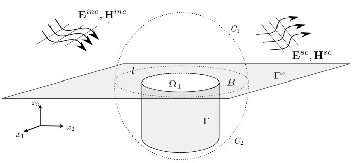
Figure 1: A cavity $\Omega_{1}$ in a perfectly conducting half-space $x_{3}\geq 0$, with boundary $\Gamma$. The surfaces $C_{1}$ and $C_{2}$ define the two halves of a sphere $C$ which is sufficiently large to contain the cavity and a finite buffer region, denoted by $B$, in the $x_{1}x_{2}$-plane beyond the edge of the cavity. The curve $\ell$ denotes the outer edge of the buffer region $B$. The unbounded half-space boundary outside of $C$ is denoted by $\Gamma^{c}$.

Suppose now that a perfectly conducting cavity $\Omega_{1}$ extends into the lower half-space $x_{3}<0$, as depicted in Figure 1. See the caption of Figure 1 for a description of the geometrical setup. The region in the lower half-space with boundary $\Gamma\cup B\cup\Gamma^{c}$ is assumed to be perfectly conducting. Given a time harmonic incident field $(\tilde{\mathbf{E}}^{\text{inc}},\tilde{\mathbf{H}}^{\text{inc}})$ with an implicit time dependence of $e^{-i\omega t}$, we seek to find the scattered field $(\tilde{\mathbf{E}}^{\text{sc}},\tilde{\mathbf{H}}^{\text{sc}})$ so that the total field

$$\tilde{\mathbf{E}}=\tilde{\mathbf{E}}^{\text{inc}}+\tilde{\mathbf{E}}^{\text{sc}},\quad\tilde{\mathbf{H}}=\tilde{\mathbf{H}}^{\text{inc}}+\tilde{\mathbf{H}}^{\text{sc}}$$

satisfies the the Maxwell equations

$$\nabla\times\tilde{\mathbf{E}}-i\omega\mu\,\tilde{\mathbf{H}} =0,$$

$$\nabla\times\tilde{\mathbf{H}}+i\omega\varepsilon\,\tilde{\mathbf{E}} =0$$

for $\mathbf{x}\in\mathbb{R}^{3+}\cup\Omega_{1}$. The material parameters are given by $\varepsilon$, the electric permittivity, and $\mu$, the magnetic permeability. Assuming $\varepsilon$ and $\mu$ are constant, it is convenient to denote suitably normalized fields by $\mathbf{E}=\sqrt{\varepsilon}\tilde{\mathbf{E}}$, $\mathbf{H}=\sqrt{\mu}\tilde{\mathbf{H}}$, etc., leading to a simpler form of Maxwell’s equations

$$\nabla\times\mathbf{E}-ik\,\mathbf{H} =0,$$ (2.1)

$$\nabla\times\mathbf{H}+ik\,\mathbf{E} =0,$$

where $k=\omega\sqrt{\mu\varepsilon}$ is known as the wavenumber. We assume that $\Re(k)>0$ and $\Im{(k)}\geq 0$. For perfect conductors, it is well-known [papas] that the tangential electric field must satisfy the boundary conditions

$$\mathbf{n}\times\mathbf{E}=\mathbf{0}\quad\text{on }\Gamma^{c}\cup\Gamma,$$ (2.2)

where $\mathbf{n}$ is the interior normal direction along $\Gamma^{c}\cup\Gamma$. The scattered field must also satisfy the Silver-Müller radiation condition:

$$\lim_{|\mathbf{x}|\rightarrow\infty}\frac{1}{|\mathbf{x}|}\left(\mathbf{H^{\text{sc}}}\times\frac{\mathbf{x}}{|\mathbf{x}|}-\mathbf{E^{\text{sc}}}\right)=0.$$ (2.3)

Remark 1.

In the following derivations and computations, we assume that the incident field $(\mathbf{E^{\text{inc}}},\mathbf{H^{\text{inc}}})$ is defined so that it satisfies not only Maxwell’s equations, but also the tangential boundary condition $\mathbf{n}\times\mathbf{E^{\text{inc}}}=\mathbf{0}$ on the entire half-space $x_{3}=0$. This is easy to accomplish by reflection and discussed in more detail in Section 6.

Before discussing the solution of the cavity problem itself, we introduce some necessary notation. Given a tangential vector field $\mathbf{j}$ along some surface $\Gamma$, the vector potential is defined by the single-layer potential

$$\mathcal{S}_{\Gamma}\mathbf{j}(\mathbf{x})=\int_{\Gamma}G(\mathbf{x},\mathbf{y})\,\mathbf{j}(\mathbf{y})\,dA_{y},$$ (2.4)

where $G(\mathbf{x},\mathbf{y})$ is the Green’s function for the three-dimensional Helmholtz equation

$$G(\mathbf{x},\mathbf{y})=\frac{e^{ik|\mathbf{x}-\mathbf{y}|}}{4\pi|\mathbf{x}-\mathbf{y}|}.$$ (2.5)

It is well known [papas] that in the case where $\mathbf{j}=\mathbf{J}$, a physical electric current, then the corresponding electric and magnetic fields generated by $\mathbf{J}$ are given by

$$\mathbf{E} =-\frac{1}{ik}\nabla\times\nabla\times\mathcal{S}_{\Gamma}\mathbf{J},$$ (2.6)

$$\mathbf{H} =\nabla\times\mathcal{S}_{\Gamma}\mathbf{J}.$$

Likewise, if $\mathbf{j}=\mathbf{M}$, a surface magnetic current, then the electric and magnetic fields induced by $\mathbf{M}$ are given by the vector anti-potentials

$$\mathbf{E}^{\text{a}} =\nabla\times\mathcal{S}_{\Gamma}\mathbf{M},$$ (2.7)

$$\mathbf{H}^{\text{a}} =\frac{1}{ik}\nabla\times\nabla\times\mathcal{S}_{\Gamma}\mathbf{M}.$$

Due to the linearity of Maxwell’s equations, any linear combination of electric current-like variable $\mathbf{j}$ and magnetic current-like variable $\mathbf{m}$ will generate a Maxwellian field

$$\mathbf{E}(\mathbf{j},\mathbf{m}) =\alpha\mathbf{E}(\mathbf{j})+\beta\mathbf{E}^{\text{a}}(\mathbf{m}),$$ (2.8)

$$\mathbf{H}(\mathbf{j},\mathbf{m}) =\alpha\mathbf{H}(\mathbf{j})+\beta\mathbf{H}^{\text{a}}(\mathbf{m}).$$

Only when $\beta=0$ does $\mathbf{j}$ correspond directly to the physical electric current. In order to develop a well-conditioned integral equation for the cavity problem, we will make use of both potentials and anti-potentials in the representation. Boundary conditions will then determine the values of $\mathbf{j}$ and $\mathbf{m}$. Such an approach is sometimes called the indirect-method since the unknowns are not the fields themselves.

2.1 A simpler problem: The bump

It is first worth considering the simpler problem where the defect in the half-space boundary is a compactly-supported bump instead of a cavity (Fig. 2). This problem can be solved using standard integral equations and the method of images. We need only satisfy boundary condition (2.2), which we write in the form:

$$\mathbf{n}\times\mathbf{E^{\text{sc}}}=-\mathbf{n}\times\mathbf{E^{\text{inc}}}.$$ (2.9)

Since, by assumption, $\mathbf{n}\times\mathbf{E^{\text{inc}}}=\mathbf{0}$ away from the bump, we need only satisfy condition (2.9) on the bump itself as long as we can construct a representation for $\mathbf{E^{\text{sc}}}$ that satisfies $\mathbf{n}\times\mathbf{E^{\text{sc}}}=\mathbf{0}$ away from the bump. To this end, we can define

$$\mathbf{E^{\text{sc}}}=\nabla\times\mathcal{S}_{\Gamma}\mathbf{M}+\nabla\times\mathcal{S}_{\Gamma_{R}}\mathbf{M}_{R}$$ (2.10)

and

$$\mathbf{H^{\text{sc}}}=\frac{1}{ik}\nabla\times\nabla\times\mathcal{S}_{\Gamma}\mathbf{M}+\frac{1}{ik}\nabla\times\nabla\times\mathcal{S}_{\Gamma_{R}}\mathbf{M}_{R}.$$ (2.11)

Here, $\Gamma_{R}$ is the reflection of the bump $\Gamma$ across the $x_{1}x_{2}$-plane. If at a point $\mathbf{x}=(a,b,c)\in\Gamma$, the magnetic current $\mathbf{M}$ is given by $\mathbf{M}{(\mathbf{x})}=(m_{1},m_{2},m_{3})$, then its image point on $\Gamma_{R}$ is $\mathbf{x}^{\prime}=(a,b,-c)$ and the image current is defined as $\mathbf{M}_{R}{(\mathbf{x}^{\prime})}=(m_{1},m_{2},-m_{3})$. It is straightforward to verify from (2.10) that $\mathbf{n}\times\mathbf{E^{\text{sc}}}=\mathbf{0}$ away from the bump (i.e., wherever $\mathbf{n}=(0,0,1)$. From standard jump condition relations, taking the limit of (2.10) to the boundary, it remains only to solve the boundary integral equation for $\mathbf{M}$:

$$\frac{1}{2}\mathbf{M}+\mathbf{n}\times\nabla\times\mathcal{S}_{\Gamma}\mathbf{M}+\mathbf{n}\times\nabla\times\mathcal{S}_{\Gamma_{R}}\mathbf{M}_{R}=-n\times\mathbf{E^{\text{inc}}}$$

on $\Gamma$, where the integral operators are understood in their principal value sense. This is a second-kind (although not resonance-free) integral equation for a smooth bump.

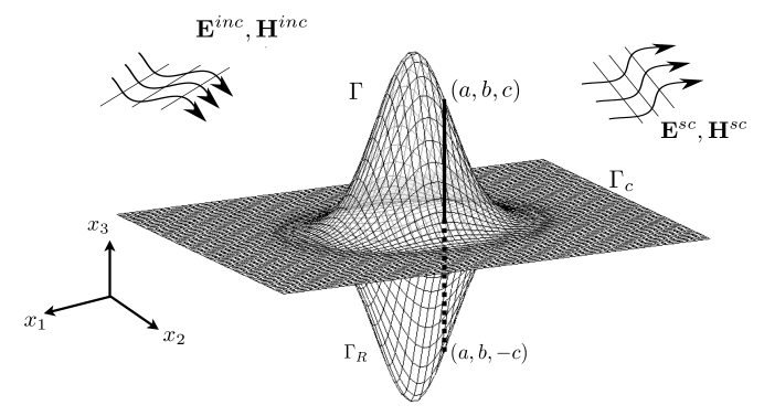
Figure 2: A bump $\Gamma$ on a perfectly conducting half-space $x_{3}\geq 0$. $\Gamma_{R}$ denotes the reflection of the bump across the $x_{1}x_{2}$-plane. The unbounded half-space boundary beyond $\Gamma$ is denoted by $\Gamma_{c}$.

2.2 The cavity case

Unfortunately, in the case of cavity deviations from a half-space, a more complicated representation is required. In order to make use of the method of images, following the approach of [JL2014], we introduce an artificial boundary $C_{1}$ that covers the cavity, as shown in Fig. 1. The boundary $C_{1}$ must be sufficiently large so that its reflection $C_{2}$ across the $x_{1}x_{2}$-plane does not intersect the cavity. The domain $\mathbb{R}^{3+}\cup\Omega_{1}$ is now decomposed into two sub-domains.

Definition 1.

In a slight abuse of notation, we will continue to use $\Omega_{1}$ to denote the interior domain, bounded by $\Gamma$, $B$ and $C_{1}$. We will refer to the upper half-space outside of $\Omega_{1}$ as the exterior domain.

In the remainder of this paper, we will denote by $(\mathbf{E^{\text{int}}},\mathbf{H^{\text{int}}})$ and $(\mathbf{E^{\text{ext}}},\mathbf{H^{\text{ext}}})$ the scattered fields in the interior and exterior domains, respectively. The exterior scattered field $(\mathbf{E^{\text{ext}}},\mathbf{H^{\text{ext}}})$ must satisfy Maxwell’s equations (2.1) in $\mathbb{R}^{3+}\backslash\Omega_{1}$, together with the boundary condition

$$\mathbf{n}\times\mathbf{E^{\text{ext}}}=\mathbf{0}\quad\text{on }\Gamma^{c}$$ (2.12)

and the interface (or transmission) conditions on $C_{1}$:

$$\mathbf{n}\times\mathbf{E^{\text{ext}}} =\mathbf{n}\times\mathbf{E^{\text{int}}},$$ (2.13)

$$\mathbf{n}\times\mathbf{H^{\text{ext}}} =\mathbf{n}\times\mathbf{H^{\text{int}}}.$$

Remark 2.

Since the domain $\Omega_{1}$ contains edges, the fields $\mathbf{E^{\text{int}}}$ and $\mathbf{H^{\text{int}}}$ in $\Omega_{1}$ are defined in the Sobolev space

$$H(curl,\Omega_{1})=\{\mathbf{u}\in(L^{2}(\Omega_{1}))^{3},\nabla\times\mathbf{u}\in(L^{2}(\Omega_{1}))^{3}\},$$

where $(L^{2}(\Omega_{1}))^{3}$ denotes the space of component-wise square-integrable vector fields in $\Omega_{1}$. Moreover, the resulting integral equations we will derive are consisted by Fredholm operators of index zero in the trace space of $H(curl,\Omega_{1})$ , for which the Fredholm alternative still applies, i.e. uniqueness implies existence. We will omit the proof but refer the reader to [BCS2002, KH2015] for a detailed discussion.

As in the case of the bump, above, we can ensure that (2.12) is satisfied using the method of images. In particular, we now represent the exterior fields by

$$\mathbf{E^{\text{ext}}} =-\frac{1}{ik}\nabla\times\nabla\times\mathcal{S}_{C_{1}}^{H}\mathbf{J}+\nabla\times\mathcal{S}_{C_{1}}^{H}\mathbf{M}+\nabla\times\mathcal{S}_{B}\mathbf{M},$$ (2.14)

$$\mathbf{H^{\text{ext}}} =\frac{1}{ik}\nabla\times\mathbf{E^{\text{ext}}}$$

$$=\nabla\times\mathcal{S}_{C_{1}}^{H}\mathbf{J}+\frac{1}{ik}\nabla\times\nabla\times\mathcal{S}_{C_{1}}^{H}\mathbf{M}+\frac{1}{ik}\nabla\times\nabla\times\mathcal{S}_{B}\mathbf{M},$$

where image fields are given by

$$\nabla\times\nabla\times\mathcal{S}_{C_{1}}^{H}\mathbf{J} =\nabla\times\nabla\times\mathcal{S}_{C_{1}}\mathbf{J}+\nabla\times\nabla\times\mathcal{S}_{C_{2}}\mathbf{J}_{R},$$ (2.15)

$$\nabla\times\mathcal{S}_{C_{1}}^{H}\mathbf{M} =\nabla\times\mathcal{S}_{C_{1}}\mathbf{M}+\nabla\times\mathcal{S}_{C_{2}}\mathbf{M}_{R}.$$

The surface currents $\mathbf{J}_{R}$ and $\mathbf{M}_{R}$ on $C_{2}$ are the images of the currents $\mathbf{J}$ and $\mathbf{M}$ on $C_{1}$. More specifically, given $\mathbf{x}=(x,y,z)\in C_{1}$ and its image point $\mathbf{x}^{\prime}=(x,y,-z)\in C_{2}$, the image currents are defined by

$$\mathbf{J}{(\mathbf{x}^{\prime})} =(-j_{1},-j_{2},j_{3}) \text{if }\mathbf{J}{(\mathbf{x})}=(j_{1},j_{2},j_{3}),$$ (2.16)

$$\mathbf{M}{(\mathbf{x}^{\prime})} =(m_{1},m_{2},-m_{3}) \text{if }\mathbf{M}{(\mathbf{x})}=(m_{1},m_{2},m_{3}).$$

It is straightforward to verify that (2.12) is enforced by symmetry. Note that the last term in the electric field representation in (2.14) does not involve an image current. However, observe that $B$ is part of the half-space boundary. It is easy to check that for any point beyond $C_{1}$, sources defined on $B$ make no contribution to the tangential electric field on $\Gamma^{c}$.

Remark 3.

We have introduced a magnetic current on $B$ even though $B$ is not part of the boundary of the exterior domain. This representation leads to a cancellation of hypersingular terms in the integral equation at the triple-junction where $C_{1}$, $C_{2}$, and $B$ intersect, and hence to a bounded integral operator. This technique, which includes layer potentials on extra boundary components to alter the kernels in the integral equation is sometimes called the global density technique. For a more detailed discussion, see [GL2012, GHL2014, JL2014].

For the interior scattered fields, we let

$$\mathbf{E^{\text{int}}} =-\frac{1}{ik}\nabla\times\nabla\times\mathcal{S}_{C_{1}}^{H}\mathbf{J}+\nabla\times\mathcal{S}_{C_{1}}^{H}\mathbf{M}+\nabla\times\mathcal{S}_{B\cup\Gamma}\mathbf{M},$$ (2.17)

$$\mathbf{H^{\text{int}}} =\frac{1}{ik}\nabla\times\mathbf{E^{\text{int}}}$$

$$=\nabla\times\mathcal{S}_{C_{1}}^{H}\mathbf{J}+\frac{1}{ik}\nabla\times\nabla\times\mathcal{S}_{C_{1}}^{H}\mathbf{M}+\frac{1}{ik}\nabla\times\nabla\times\mathcal{S}_{B\cup\Gamma}\mathbf{M}.$$

Note that the only difference in the interior representation when compared with the exterior representation is that we have included a contribution from a magnetic current on the cavity $\Gamma$. Although $C_{2}$, the image surface of $C_{1}$, is not part of the boundary of $\Omega_{1}$, its contribution is added to the interior scattered fields by the similar reason as in Remark 3.

For convenience, given two surfaces $\Gamma_{s}$ and $\Gamma_{t}$, and the current $\mathbf{J}$ on $\Gamma_{s}$, we define the following two surface vector potentials for $\mathbf{x}\in\Gamma_{t}$ by

$$\mathcal{K}_{\Gamma_{t},\Gamma_{s}}\mathbf{J}(\mathbf{x}) =\mathbf{n}(\mathbf{x})\times\frac{1}{ik}\nabla\times\nabla\times\mathcal{S}_{\Gamma_{s}}\mathbf{J}(\mathbf{x}),$$ (2.18)

$$\mathcal{N}_{\Gamma_{t},\Gamma_{s}}\mathbf{J}(\mathbf{x}) =\mathbf{n}(\mathbf{x})\times\nabla\times\mathcal{S}_{\Gamma_{s}}\mathbf{J}(\mathbf{x}).$$ (2.19)

When $\Gamma_{s}$ has a reflection, we define $\mathcal{K}^{H}_{\Gamma_{t},\Gamma_{s}}\mathbf{J}$ and $\mathcal{N}^{H}_{\Gamma_{t},\Gamma_{s}}\mathbf{J}$ to include the contribution from the reflected image currents as well, as in (2.15).

When $\Gamma_{t}=\Gamma_{s}=\Gamma$, the integral operators $\mathcal{K}$ and $\mathcal{N}$ become singular. More precisely, the integral in $\mathcal{K}_{\Gamma,\Gamma}$ is hypersingular and defined in the Hadamard principal-value sense, while $\mathcal{N}_{\Gamma,\Gamma}$ is defined in the Cauchy principal-value sense [Cot2]. In this case, the following jump relations hold:

$$\lim_{\mathbf{x}\rightarrow\Gamma^{\pm}}\mathbf{n}(\mathbf{x})\times\frac{1}{ik}\nabla\times\nabla\times\mathcal{S}_{\Gamma}\mathbf{J}(\mathbf{x}) =\mathcal{K}_{\Gamma,\Gamma}\mathbf{J}(\mathbf{x}),$$ (2.20)

$$\lim_{\mathbf{x}\rightarrow\Gamma^{\pm}}\mathbf{n}(\mathbf{x})\times\nabla\times\mathcal{S}_{\Gamma}\mathbf{J}(\mathbf{x}) =\frac{1}{2}\mathbf{J}(\mathbf{x})\pm\mathcal{N}_{\Gamma,\Gamma}\mathbf{J}(\mathbf{x}),$$ (2.21)

where $\Gamma^{\pm}$ denotes the side that corresponds to the outward ($+$) or inward ($-$) normal, respectively.

Using the previous integral representations for the interior and exterior fields, the boundary value problem

$$\nabla\times\mathbf{E}-ik\,\mathbf{H} =0, \text{in }\Omega_{1}\cup\mathbb{R}^{3+},$$ (2.22)

$$\nabla\times\mathbf{H}+ik\,\mathbf{E} =0, \text{in }\Omega_{1}\cup\mathbb{R}^{3+},$$

$$\mathbf{n}\times\mathbf{E^{\text{ext}}} =\mathbf{n}\times\mathbf{E^{\text{int}}}, \text{on }C_{1},$$

$$\mathbf{n}\times\mathbf{H^{\text{ext}}} =\mathbf{n}\times\mathbf{H^{\text{int}}}, \text{on }C_{1},$$

$$\mathbf{n}\times\mathbf{E^{\text{int}}} =-\mathbf{n}\times\mathbf{E^{\text{inc}}} \text{on }B\cup\Gamma,$$

along with jump conditions (2.20) and (2.21), immediately yields a system of integral equations for $\mathbf{J}$ and $\mathbf{M}$:

$$\mathbf{M}-\mathcal{N}_{C_{1},\Gamma}\mathbf{M} =\mathbf{0} \text{on }C_{1},$$ (2.23)

$$\mathbf{J}-\mathcal{K}_{C_{1},\Gamma}\mathbf{M} =\mathbf{0} \text{on }C_{1},$$

$$\frac{1}{2}\mathbf{M}+\mathcal{N}_{B,\Gamma}\mathbf{M} =\mathbf{0} \text{on }B,$$

$$\frac{1}{2}\mathbf{M}-\mathcal{K}^{H}_{\Gamma,C_{1}}\mathbf{J}+\mathcal{N}^{H}_{\Gamma,C_{1}}\mathbf{M}+\mathcal{N}_{\Gamma,B\cup\Gamma}\mathbf{M} =-\mathbf{n}\times\mathbf{E^{\text{inc}}} \text{on }\Gamma.$$

Due to the existence of corners, the integral system (2.23) is not second kind Fredholm equation. Nevertheless, the system is well conditioned once the corner singularity is well resolved numerically.

Remark 4.

Given the magnetic current $\mathbf{M}$ along $\Gamma$, the first three equations the system (2.23) are explicitly solvable because they only involve the application of an off-surface layer potential. Therefore, our formulation can be reduced to an unknown magnetic current $\mathbf{M}$ along $\Gamma$ only. In particular, by substitition of the first three equations in (2.23) into the fourth equation in (2.23), we have the integral equation

$$\frac{1}{2}\mathbf{M}-\mathcal{K}^{H}_{\Gamma,C_{1}}\mathcal{K}_{C_{1},\Gamma}\mathbf{M}+\mathcal{N}^{H}_{\Gamma,C_{1}}\mathcal{N}_{C_{1},\Gamma}\mathbf{M}-2\mathcal{N}_{\Gamma,B}\mathcal{N}_{B,\Gamma}\mathbf{M}+\mathcal{N}_{\Gamma,\Gamma}\mathbf{M}=-\mathbf{n}\times\mathbf{E^{\text{inc}}}$$ (2.24)

for $\mathbf{M}$ along $\Gamma$. Not only does this observation reduce the number of unknowns significantly, it will play a key role in avoiding low-frequency breakdown in the electric field, as shown in Section 4.

3 Existence and uniquness

Since the integral system (2.23) consists of Fredholm operators of index zero, by the Fredholm alternative, existence follows from uniqueness. This is given by the following theorem.

Theorem 3.1.

Equation (2.23) admits a unique solution $\mathbf{J}$ and $\mathbf{M}$ for $k>0$.

Proof.

It suffices to show that the system (2.23) has only the trivial solution for $k>0$. For this, let us denote by $\Omega_{2}$ the region bounded by $C_{2}$, $\Gamma$ and $B$. The proof involves three steps.

First, for $\mathbf{J}$ and $\mathbf{M}$ given in (2.23), define the induced electromagnetic field $(\mathbf{E},\mathbf{H})$ for $\mathbf{x}\in\mathbb{R}^{3}\backslash(\Omega_{1}\cup\Omega_{2})$ by

$$\mathbf{E} =-\frac{1}{ik}\nabla\times\nabla\times\mathcal{S}_{C_{1}}^{H}\mathbf{J}+\nabla\times\mathcal{S}_{C_{1}}^{H}\mathbf{M}+\nabla\times\mathcal{S}_{B}\mathbf{M},$$ (3.1)

$$\mathbf{H} =\nabla\times\mathcal{S}_{C_{1}}^{H}\mathbf{J}+\frac{1}{ik}\nabla\times\nabla\times\mathcal{S}_{C_{1}}^{H}\mathbf{M}+\frac{1}{ik}\nabla\times\nabla\times\mathcal{S}_{B}\mathbf{M},$$

and for $\mathbf{x}\in\Omega_{1}\cup\Omega_{2}$,

$$\mathbf{E} =-\frac{1}{ik}\nabla\times\nabla\times\mathcal{S}_{C_{1}}^{H}\mathbf{J}+\nabla\times\mathcal{S}_{C_{1}}^{H}\mathbf{M}+\nabla\times\mathcal{S}_{B\cup\Gamma}\mathbf{M},$$ (3.2)

$$\mathbf{H} =\nabla\times\mathcal{S}_{C_{1}}^{H}\mathbf{J}+\frac{1}{ik}\nabla\times\nabla\times\mathcal{S}_{C_{1}}^{H}\mathbf{M}+\frac{1}{ik}\nabla\times\nabla\times\mathcal{S}_{B\cup\Gamma}\mathbf{M}.$$

From (2.23), we have that

$$\lim_{{\begin{subarray}{c}\mathbf{x}\rightarrow\Gamma^{c}\\ \mathbf{x}\in\mathbb{R}^{3}\backslash(\Omega_{1}\cup\Omega_{2})\end{subarray}}}\mathbf{n}\times\mathbf{E}=0,\qquad\lim_{\begin{subarray}{c}\mathbf{x}\rightarrow B\cup\Gamma\\ \mathbf{x}\in\Omega_{1}\end{subarray}}\mathbf{n}\times\mathbf{E}=0$$ (3.3)

and

$$[\mathbf{n}\times\mathbf{E}]=0,\quad[\mathbf{n}\times\mathbf{H}]=0\quad\text{on }C_{1},$$ (3.4)

where $[\cdot]$ denotes the jump in the corresponding the field.

Let $D\subset\mathbb{R}^{3+}$ be a finite region that is bounded by a sufficiently large hemisphere $\partial D$ and the surfaces $\Gamma^{c}$ and $C_{1}$. Applying Green’s first vector identity [Cot2] to $\mathbf{E}$ and its complex conjugate $\overline{\mathbf{E}}$ in $D$, and recalling the fact that $\nabla\cdot\mathbf{E}=0$ in this region yields

$$\int_{\partial D\cup C_{1}}(\mathbf{n}\times\mathbf{E})\cdot(\nabla\times\overline{\mathbf{E}})\,dA=\iint_{D}\left(|\nabla\times\mathbf{E}|^{2}-k^{2}|\mathbf{E}|^{2}\right)\,dV.$$ (3.5)

Similarly, applying the same identity to $\mathbf{E}$ in $\Omega_{1}$, we have

$$\int_{C_{1}\cup\Gamma}(\mathbf{n}\times\mathbf{E})\cdot(\nabla\times\overline{\mathbf{E}})\,dA=\iint_{\Omega_{1}}\left(|\nabla\times\mathbf{E}|^{2}-k^{2}|\mathbf{E}|^{2}\right)\,dV.$$ (3.6)

Note that $\mathbf{n}$ in (3.5) and (3.6) denotes the exterior normal with respect to the regions $D$ and $\Omega_{1}$, and that the right hand side of both relations is purely real (for real $k$). Combining (3.5) and (3.6), using the continuity condition (3.4) along $C_{1}$, and taking imaginary parts we have

$$\Im{\int_{\partial D}\left(\mathbf{n}\times\mathbf{E}\right)\cdot\left(\nabla\times\overline{\mathbf{E}}\right)}=\Im{\int_{\Gamma}\left(\mathbf{n}\times\mathbf{E}\right)\cdot\left(\nabla\times\overline{\mathbf{E}}\right)}=0,$$ (3.7)

where $\Im$ denotes the imaginary part. Lastly, since $\mathbf{n}\times\mathbf{E}=0$ on $\Gamma$, relation (3.7) implies that the electric field is identically zero in $D$ by Rellich’s lemma [Cot2]. By analytic continuation from $C_{1}$ into $\Omega_{1}$, we also obtain $\mathbf{E}=0$ and $\mathbf{H}=0$ in $\Omega_{1}$.

The second step in the proof is to show that the fields $(\mathbf{E},\mathbf{H})$ in $\Omega_{2}$ satisfy the following boundary conditions

$$\mathbf{n}\times\mathbf{E} =\mathbf{M} \text{on }\Gamma\cup B,$$ (3.8)

$$\mathbf{n}\times\mathbf{H} =\mathbf{0} \text{on }\Gamma\cup B,$$

$$\mathbf{n}\times\mathbf{E} =\mathcal{N}_{C_{2},\Gamma^{\prime}}\mathbf{M}+\mathcal{N}_{C_{2},\Gamma}\mathbf{M} \text{on }C_{2},$$

$$\mathbf{n}\times\mathbf{H} =\mathcal{K}_{C_{2},\Gamma^{\prime}}\mathbf{M}+\mathcal{K}_{C_{2},\Gamma}\mathbf{M} \text{on }C_{2}.$$

Here, just to clarify, $\mathbf{n}$ on $\Gamma\cup B$ is the exterior normal with respect to $\Omega_{1}$ and $\mathbf{n}$ on $C_{2}$ is the exterior normal with respect to $\Omega_{2}$. The surface $\Gamma^{\prime}$ is the image of $\Gamma$ with respect to the $x_{1}x_{2}$-plane, and $\mathbf{M}$ on $\Gamma^{\prime}$ is the corresponding image magnetic current. By (3.1), (3.2), and the jump relations (2.20), (2.21), we have that

$$[\mathbf{n}\times\mathbf{E}]=-\mathbf{M}\quad\text{and}\quad[\mathbf{n}\times\mathbf{H}]=0\quad\text{on }\Gamma\cup B.$$ (3.9)

Using the fact that $\mathbf{E}=\mathbf{0}$ and $\mathbf{H}=\mathbf{0}$ in $\Omega_{1}$, we obtain the desired boundary conditions (3.8) on $\Gamma\cup B$ for the fields $(\mathbf{E},\mathbf{H})$ in $\Omega_{2}$.

Turning to the boundary $C_{2}$, we have the jump conditions

$$[\mathbf{n}\times\mathbf{E}]=-\mathbf{M}^{\prime}+\mathcal{N}_{C_{2},\Gamma}\mathbf{M}\quad\text{and}\quad[\mathbf{n}\times\mathbf{H}]=-\mathbf{J}^{\prime}+\mathcal{K}_{C_{2},\Gamma}\mathbf{M}\quad\text{on }C_{2}.$$ (3.10)

Here, $\mathbf{J}^{\prime}$ and $\mathbf{M}^{\prime}$ are the image surface currents on $C_{2}$. By equation (2.23) and symmetry,

$$\mathbf{M}^{\prime}=\mathcal{N}_{C_{2},\Gamma^{\prime}}\mathbf{M}^{\prime}\quad\text{and}\quad\mathbf{J}^{\prime}=\mathcal{K}_{C_{2},\Gamma^{\prime}}\mathbf{M}^{\prime}\quad\text{on }C_{2},$$ (3.11)

where $\mathbf{M}^{\prime}$ on $\Gamma^{\prime}$ is again the image magnetic current of $\mathbf{M}$ on $\Gamma$. Combining (3.10) and (3.11), we obtain the remaining boundary conditions in (3.8).

The third, and final, step in the proof is to show that the electromagnetic field satisfying (3.8) is identically zero. For this, extend $\mathbf{E}$ and $\mathbf{H}$ from $\Omega_{2}$ to $\mathbb{R}^{3-}\backslash\Omega_{2}$ by letting

$$\mathbf{E} =-\nabla\times\mathcal{S}_{\Gamma^{\prime}}\mathbf{M}^{\prime}+\nabla\times\mathcal{S}_{\Gamma}\mathbf{M}$$ (3.12)

$$\mathbf{H} =-\frac{1}{ik}\nabla\times\nabla\times\mathcal{S}_{\Gamma^{\prime}}\mathbf{M}^{\prime}+\frac{1}{ik}\nabla\times\nabla\times\mathcal{S}_{\Gamma}\mathbf{M}.$$

It is easy to see that $(\mathbf{E},\mathbf{H})$ is an electromagnetic field satisfying

$$\mathbf{n}\times\mathbf{H}=\mathbf{0}\quad\text{on }\Gamma^{c}.$$ (3.13)

Following the same argument as in the first step (with $\mathbf{E}$ and $\mathbf{H}$ exchanged), we must have $\mathbf{E}=\mathbf{0}$ and $\mathbf{H}=\mathbf{0}$ in $\Omega_{2}$, which implies $\mathbf{M}=\mathbf{0}$ on $\Gamma$. Therefore, by (2.23), we obtain $\mathbf{J}=\mathbf{0}$ and $\mathbf{M}=\mathbf{0}$ on $C_{1}$.
∎

A similar proof can be obtained in the case where $\Re(k)>0$ and $\Im(k)>0$. In the static case where $k=0$, our representation is not valid and must be altered. However, the existence and uniqueness can be handled directly by electro- and magneto-static arguments.

4 Low-frequency breakdown

It is clear that the integral representations (2.14) and (2.17) are numerically unstable as $k\rightarrow 0$ due to the explicit $1/ik$ scaling. This problem is not intrinsic to the Maxwell system (2.1), where the electric and magnetic field simply uncouple in the static limit. Rather, it is due to the use of vector currents $\mathbf{J}$, $\mathbf{M}$ as the unknowns. The resulting loss of precision is generally referred to as low-frequency breakdown [ZC2000]. Rather than develop a new mathematical formalism to overcome this, as in [EG10, EG13], we modify our method described above to create a representation that is stable as $k\rightarrow 0$. In short, using properties of the electromagnetic fields and vector identities, we are able to express the electric field only in terms of $\mathbf{M}$, and in the process, eliminate the terms which scale as $1/ik$. The magnetic field representation still formally suffers from low-frequency breakdown, but numerically it is relatively benign as $k\to 0$.

In order to express $\mathbf{E}$ only in terms of well-scaled operators of $\mathbf{M}$, we require the following identity.

Lemma 4.1.

Let $\Gamma$ be an open surface with smooth boundary $\ell$, and let $\mathbf{J}$ be a smooth tangential vector field along $\Gamma$. Then

$$\frac{1}{ik}\nabla\times\nabla\times\mathcal{S}_{\Gamma}\mathbf{J}=-ik\mathcal{S}_{\Gamma}\mathbf{J}+\nabla\mathcal{S}_{\Gamma}\left(\frac{\nabla_{\Gamma}\cdot\mathbf{J}}{ik}\right)-\nabla\mathcal{S}_{\ell}\left(\frac{\mathbf{J}\cdot\mathbf{b}}{ik}\right)$$ (4.1)

where $\mathbf{b}=\bm{\tau}\times\mathbf{n}$ is the outward bi-normal vector along $\ell$, with $\bm{\tau}$ the unit tangent vector along $\ell$ and $\mathbf{n}$ the surface normal (oriented so that $\mathbf{b}$ points away from the surface).

Proof.

Using the point-wise vector identity $\nabla\times\nabla\times{\bf a}=-\Delta{\bf a}+\nabla\nabla\cdot{\bf a}$, we have

$$\frac{1}{ik}\nabla\times\nabla\times\mathcal{S}_{\Gamma}\mathbf{J}=-\frac{1}{ik}\Delta\mathcal{S}_{\Gamma}\mathbf{J}+\nabla\nabla\cdot\mathcal{S}_{\Gamma}\left(\frac{\mathbf{J}}{ik}\right).$$ (4.2)

Since $\mathcal{S}_{\Gamma}\mathbf{J}$ is a vector-valued Helmholtz potential, it is clear that

$$-\frac{1}{ik}\Delta\mathcal{S}_{\Gamma}\mathbf{J}=-ik\mathcal{S}_{\Gamma}\mathbf{J}.$$ (4.3)

For the second term on the right-hand side of (4.2), we apply Stokes’s identity [Ned01] on the surface $\Gamma$:

$$\nabla\cdot\mathcal{S}_{\Gamma}\left(\frac{\mathbf{J}}{ik}\right) =-\int_{\Gamma}\nabla_{\mathbf{y},\Gamma}\cdot\left(G(\mathbf{x},\mathbf{y})\,\frac{\mathbf{J}(\mathbf{y})}{ik}\right)\,dA_{y}+\int_{\Gamma}G(\mathbf{x},\mathbf{y})\,\frac{\nabla_{\Gamma}\cdot\mathbf{J}(\mathbf{y})}{ik}\,dA_{y}$$ (4.4)

$$=-\mathcal{S}_{\ell}\left(\frac{\mathbf{J}\cdot\mathbf{b}}{ik}\right)+\mathcal{S}_{\Gamma}\left(\frac{\nabla_{\Gamma}\cdot\mathbf{J}}{ik}\right),$$

where $\nabla_{\mathbf{y},\Gamma}\cdot$ denotes the surface divergence with respect to the variable $\mathbf{y}$. ∎

Corollary 4.2.

Let $\Gamma$ be a surface whose boundary $\ell$ is a curve that lies on the plane $x_{3}=0$, and let $\mathbf{J}$ and $\mathbf{M}$ be surface electric and magnetic currents on $\Gamma$ with image currents defined in (2.16). Note that the image currents also lie along $x_{3}=0$. Then

$$\frac{1}{ik}\nabla\times\nabla\times\mathcal{S}^{H}_{\Gamma}\mathbf{J} =-ik\mathcal{S}^{H}_{\Gamma}\mathbf{J}+\nabla\mathcal{S}^{H}_{\Gamma}\left(\frac{\nabla_{\Gamma}\cdot\mathbf{J}}{ik}\right),$$ (4.5)

$$\frac{1}{ik}\nabla\times\nabla\times\mathcal{S}^{H}_{\Gamma}\mathbf{M} =-ik\mathcal{S}^{H}_{\Gamma}\mathbf{M}+\nabla\mathcal{S}^{H}_{\Gamma}\left(\frac{\nabla_{\Gamma}\cdot\mathbf{M}}{ik}\right)-2\nabla\mathcal{S}_{\ell}\left(\frac{\mathbf{M}\cdot\mathbf{b}}{ik}\right).$$

We can now establish the following identity:

Lemma 4.3.

For a tangential electric and magnetic currents $\mathbf{J}$, $\mathbf{M}$ along $\Gamma$, defined as in (2.17),

$$\frac{\nabla_{C_{1}}\cdot\mathbf{J}}{ik}=-\mathbf{n}\cdot\nabla\times\mathcal{S}_{\Gamma}\mathbf{M}.$$ (4.6)

Proof.

First, apply Corollary 4.2 to rewrite the representation of the electric field in the form

$$\mathbf{E^{\text{ext}}} =ik\mathcal{S}^{H}_{C_{1}}\mathbf{J}-\nabla\mathcal{S}^{H}_{C_{1}}\left(\frac{\nabla_{C_{1}}\cdot\mathbf{J}}{ik}\right)+\nabla\times\mathcal{S}_{C_{1}}^{H}\mathbf{M}+\nabla\times\mathcal{S}_{B}\mathbf{M},$$ (4.7)

$$\mathbf{E^{\text{int}}} =ik\mathcal{S}^{H}_{C_{1}}\mathbf{J}-\nabla\mathcal{S}^{H}_{C_{1}}\left(\frac{\nabla_{C_{1}}\cdot\mathbf{J}}{ik}\right)+\nabla\times\mathcal{S}_{C_{1}}^{H}\mathbf{M}+\nabla\times\mathcal{S}_{B\cup\Gamma}\mathbf{M}.$$

Taking the difference of $\mathbf{E^{\text{ext}}}$ and $\mathbf{E^{\text{int}}}$ in (4.7), computing normal components, using the jump relations for the single layer potential, and recalling the continuity condition

$$\mathbf{n}\cdot\mathbf{E^{\text{ext}}}=\mathbf{n}\cdot\mathbf{E^{\text{int}}}\quad\text{on }C_{1},$$ (4.8)

yields the desired result in (4.6). ∎

We can now derive low-frequency versions of integral equation (2.24) and representations for the electric and magnetic fields.

4.1 A modified integral equation

Using the previous results, we can now derive an integral equation along $\Gamma$ which does not suffer from low-frequency breakdown, as does equation (2.24). Inspection of the various terms in (2.24) shows that $1/ik$ scaling is present only in the term

$$-\mathcal{K}^{H}_{\Gamma,C_{1}}\mathcal{K}_{C_{1},\Gamma}\mathbf{M}.$$ (4.9)

By application of Lemma 4.1 and use of the result in Corollary 4.2, this term can be replaced as

$$-\mathcal{K}^{H}_{\Gamma,C_{1}}\mathcal{K}_{C_{1},\Gamma}\mathbf{M}=\mathbf{n}\times ik\mathcal{S}^{H}_{C_{1}}\mathbf{J}-\mathbf{n}\times\nabla\mathcal{S}^{H}_{C_{1}}\left(\frac{\nabla_{C_{1}}\cdot\mathbf{J}}{ik}\right),$$ (4.10)

where, recalling that by equation (2.23)

$$\mathbf{J}=\mathcal{K}_{C_{1},\Gamma}\mathbf{M}=\mathbf{n}\times\left(\frac{1}{ik}\nabla\times\nabla\times\mathcal{S}_{\Gamma}\mathbf{M}\right).$$ (4.11)

Using (4.11), the first term in (4.10) can be rewritten in terms of $\mathbf{M}$ on $\Gamma$:

$$\mathbf{n}\times ikS^{H}_{C_{1}}\mathbf{J}=\mathbf{n}\times\mathcal{S}_{C_{1}}^{H}\left(\mathbf{n}\times\nabla\times\nabla\times\mathcal{S}_{\Gamma}\mathbf{M}\right).$$ (4.12)

Combining (4.12) and (4.6), we can have the modified equation along $\Gamma$:

$$\frac{1}{2}\mathbf{M}+\mathbf{n}\times\mathcal{S}_{C_{1}}^{H}\left(\mathbf{n}\times\nabla\times\nabla\times\mathcal{S}_{\Gamma}\mathbf{M}\right)+\mathbf{n}\times\nabla\mathcal{S}^{H}_{C_{1}}\left(\mathbf{n}\cdot\nabla\times\mathcal{S}_{\Gamma}\mathbf{M}\right)\\ +\mathcal{N}^{H}_{\Gamma,C_{1}}\mathcal{N}_{C_{1},\Gamma}\mathbf{M}-2\mathcal{N}_{\Gamma,B}\mathcal{N}_{B,\Gamma}\mathbf{M}+\mathcal{N}_{\Gamma,\Gamma}\mathbf{M}=-\mathbf{n}\times\mathbf{E^{\text{inc}}}.$$ (4.13)

This is equivalent to (2.24), but is clearly immune from low-frequency breakdown.

4.2 Field calculations

Furthermore, given the solution $\mathbf{M}$ to integral equation (4.13), we have the following representations for the electric field which do not suffer from low-frequency breakdown:

$$\mathbf{E^{\text{ext}}} =ik\mathcal{S}^{H}_{C_{1}}\mathcal{K}_{C_{1},\Gamma}\mathbf{M}-\nabla\mathcal{S}^{H}_{C_{1}}\left(\mathbf{n}\cdot\nabla\times\mathcal{S}_{\Gamma}\mathbf{M}\right)+\nabla\times\mathcal{S}_{C_{1}}^{H}\mathbf{M}+\nabla\times\mathcal{S}_{B}\mathbf{M},$$ (4.14)

$$\mathbf{E^{\text{int}}} =ik\mathcal{S}^{H}_{C_{1}}\mathcal{K}_{C_{1},\Gamma}\mathbf{M}-\nabla\mathcal{S}^{H}_{C_{1}}\left(\mathbf{n}\cdot\nabla\times\mathcal{S}_{\Gamma}\mathbf{M}\right)+\nabla\times\mathcal{S}_{C_{1}}^{H}\mathbf{M}+\nabla\times\mathcal{S}_{B\cup\Gamma}\mathbf{M}.$$

Once $\mathbf{M}$ along $\Gamma$ has been obtained by solving (4.13), we can obtain $\mathbf{M}$ on $C_{1}\cup B$ through (2.23). Evaluation via representation (4.14) is stable as $k\to 0$. On the other hand, we are left with computing the magnetic field as

$$\mathbf{H^{\text{ext}}}=\frac{1}{ik}\nabla\times\mathbf{E^{\text{ext}}},\qquad\mathbf{H^{\text{int}}}=\frac{1}{ik}\nabla\times\mathbf{E^{\text{int}}},$$ (4.15)

which are inherently first-order operations in the variable $\mathbf{M}$ and will obviously suffer from low-frequency breakdown. As an alternative, we may try to rewrite $\mathbf{H}$ using vector identities and in terms of the variable $\mathbf{J}$. In the case of $\mathbf{H^{\text{int}}}$, for example, we have

$$\mathbf{H^{\text{int}}}=\nabla\times\mathcal{S}_{C_{1}}^{H}\mathbf{J}+\frac{1}{ik}\nabla\times\nabla\times\mathcal{S}_{C_{1}}^{H}\mathbf{M}+\frac{1}{ik}\nabla\times\nabla\times\mathcal{S}_{B\cup\Gamma}\mathbf{M}.$$ (4.16)

The expression for $\mathbf{H^{\text{ext}}}$ is nearly identical. Any attempt using the previous lemmas or corollary to simplify this representation will require the (numerical) evaluation of the quantities $\mathbf{J}$, $\nabla_{\Gamma}\cdot\mathbf{M}/ik$, and $\mathbf{M}\cdot\mathbf{b}/ik$. Empirically, these expressions can be evaluated at the cost of a mild loss of numerical precision. The quantity $\mathbf{J}$ can be directly evaluated via $\mathbf{J}=\mathcal{K}_{C_{1},\Gamma}\mathbf{M}$, or by using the identity:

$$\mathbf{J}=\mathbf{n}\times\left(-ik\mathcal{S}_{\Gamma}\mathbf{M}+\nabla\mathcal{S}_{\Gamma}\left(\frac{\nabla_{\Gamma}\cdot\mathbf{M}}{ik}\right)-\nabla\mathcal{S}_{\ell}\left(\frac{\mathbf{M}\cdot\mathbf{b}}{ik}\right)\right).$$ (4.17)

We compute the function $\rho_{M}=\nabla_{\Gamma}\cdot\mathbf{M}/ik$ merely by spectral differentiation in a $10^{\text{th}}$-order Legendre discretization, and the term $\phi_{M}=\mathbf{M}\cdot\mathbf{b}/ik$ by extrapolation.

These schemes lead to roughly an $\mathcal{O}(\log k)$ loss in absolute precision. For example, as discussed in the numerical examples section, for $k\approx 10^{-10}$, we are able to obtain approximately 6 digits of accuracy.

Remark 5.

The function $\phi_{M}$ cannot be evaluated naively for small $k$. Numerical experiments indicate that ${\mathbf{M}\cdot\mathbf{b}}\approx\mathcal{O}(k)$ as $k\rightarrow 0$, but we have not found a proof of this fact. Similar to $\rho_{M}$, we numerically found that $\phi_{M}$ has a low-frequency limit. In particular, we can formally expand:

$$\frac{\mathbf{M}\cdot\mathbf{b}}{ik}=m_{1}+km_{2}+\ldots.$$ (4.18)

The quantity $\phi_{M}$ can then be evaluated for several distinct non-zero values of $k$, and the coefficients $m_{j}$ can be estimated to the desired order of accuracy. These estimated values can then be used to compute $\phi_{M}$ for any $k\geq 0$. The result can then be used in (4.17) to evaluate the $\mathbf{H}$ field. This form of low-frequency breakdown is, therefore, much less pernicious than that addressed by Lemma 4.3, and that present in the evaluation of $\rho_{M}$, which is sometimes referred to as dense-mesh breakdown. Nevertheless, we consider it to be an open problem to find an integral formulation which avoids the need for this asymptotic approach.

5 Separation of variables for boundary integral operators

For arbitrarily shaped cavities, a full three-dimensional treatment of quadratures and geometry discretization is required to evaluate the integral operators discussed in the previous section, not to mention schemes to solve the corresponding integral equations. While fast multipole methods reduce the computational complexity of applying such integral operators to $\mathcal{O}(N)$ or $\mathcal{O}(N\log N)$, (see for example, [Cheng2006]) and high-order quadratures have been developed for weakly-singular kernels on arbitrary surface triangulations [Bremer2012], the associated constants implicit in the $\mathcal{O}(\cdot)$ scaling are relatively large. On the other hand, for a wide class of geometries – namely those with rotational symmetry – two useful accelerations are easily obtained. First, in problems for which the Green’s function is translation invariant, one can apply separation of variables in the azimuthal angle, $\theta$, relative to the $x_{3}$-axis, and then Fourier decompose the problem. This transforms the original integral equation, defined on a surface in three dimensions, into a sequence of uncoupled integral equations (one for each Fourier mode) defined along a one-dimensional generating curve. Second, the resulting linear systems are much smaller, and the associated quadrature issues are much easier to address [HK2014, Hao2015, YHM2012, Liu2015, gedney_1990, oneil_2016]. We avoid a detailed description of axisymmetric integral equation solvers here, and instead point the reader to the previous references for discussions related to quadrature and kernel evaluation. In what follows below, we provide a brief description of the discretization relevant to our cavity scattering problem.

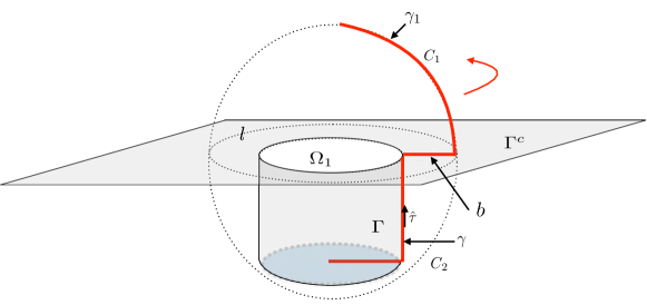
Figure 3: Axisymmetric cavity with generating curve $g=\gamma\cup b\cup\gamma_{1}$.

5.1 Modal kernels and operators

A simple example of the geometrical setup is shown in Fig. 3. A point $\mathbf{x}=(x_{1},x_{2},x_{3})$ in $\mathbb{R}^{3}$ will be denoted in the usual cylindrical coordinates as $\mathbf{x}=(r,\theta,z)$. The standard unit vectors in cylindrical coordinates will be denoted as $(\mathbf{e}_{r},\mathbf{e}_{\theta},\mathbf{e}_{z})$. The generating curve is given by $g=\gamma\cup b\cup\gamma_{1}$, which we assume is parameterized by $g(s)=(r(s),z(s))$, where $s$ denotes arclength. The tangent vector along the generating curve is then $\mathbf{t}=\frac{dr}{ds}\mathbf{e}_{r}+\frac{dz}{ds}\mathbf{e}_{z}$, and the exterior normal $\mathbf{n}$ is given by $\mathbf{n}=\frac{dz}{ds}\mathbf{e}_{r}-\frac{dr}{ds}\mathbf{e}_{z}$. Relative to the surface frame $\mathbf{t}$, $\mathbf{n}$, $\mathbf{e}_{\theta}$, any tangential vector field $\mathbf{J}$ along $\Gamma\cup B\cup C_{1}$ can be written as:

$$\mathbf{J}(s,\theta)=\sum_{m}(J_{m}^{1}(s)\,\mathbf{t}+J_{m}^{2}(s)\,\mathbf{e}_{\theta})\,e^{im\theta}.$$ (5.1)

In the scalar case, a second-kind boundary integral equation on a body of revolution $\Omega$,

$$u(\mathbf{x})+\int_{\partial\Omega_{1}}G(\mathbf{x}-\mathbf{x}^{\prime})\,u(\mathbf{x}^{\prime})\,dA(\mathbf{x}^{\prime})=f(\mathbf{x}),$$ (5.2)

can immediately be decomposed into a sequence of decoupled equations

$$u_{m}(\mathbf{x})+2\pi\int_{g}G_{m}(r,z,r^{\prime},z^{\prime})\,u_{m}(r^{\prime},z^{\prime})\,r^{\prime}\,ds(r^{\prime},z^{\prime})=f_{m}(r,z)$$ (5.3)

where

$$u(\mathbf{x}) =\sum_{m}u_{m}(r,z)\,e^{im\theta},$$ (5.4)

$$f(\mathbf{x}) =\sum_{m}f_{m}(r,z)\,e^{im\theta},$$

$$G(\mathbf{x}-\mathbf{x}^{\prime}) =\sum_{m}G_{m}(r,z,r^{\prime},z^{\prime})\,e^{im(\theta-\theta^{\prime})}.$$

However, in the vector-valued integral equation setting, the components of the unknown $\mathbf{J}$ do not fully separate when expressed in terms of local, tangential coordinates [oneil_2016]. We therefore need to compute the action of the single-layer potential operator $\mathcal{S}$, and its derivatives, on a tangential density $\mathbf{J}$. Using the fact that relative to the Cartesian unit vectors $\mathbf{e}_{1}$, $\mathbf{e}_{2}$, $\mathbf{e}_{3}$:

$$\mathbf{e}_{r} =\cos\theta\,\mathbf{e}_{1}+\sin\theta\,\mathbf{e}_{2},$$ (5.5)

$$\mathbf{e}_{\theta} =-\sin\theta\,\mathbf{e}_{1}+\cos\theta\,\mathbf{e}_{2},$$

$$\mathbf{e}_{z} =\mathbf{e}_{3},$$

it is straightforward to verify that if $\mathbf{J}$ is as in (5.1), then

$$\mathcal{S}_{\Gamma}\mathbf{J}=\sum_{m}\left(c_{m}^{1}\mathbf{e}_{r}+c_{m}^{2}\mathbf{e}_{\theta}+c_{m}^{3}\mathbf{e}_{z}\right)\,e^{im\theta}$$ (5.6)

where

$$c_{m}^{1} =\int_{\gamma}G_{m}^{\cos}(r,z,r^{\prime},z^{\prime})\,J^{1}_{m}(s)\,\frac{dr^{\prime}}{ds}\,r^{\prime}\,ds-i\int_{\gamma}G_{m}^{\sin}(r,z,r^{\prime},z^{\prime})\,J^{2}_{m}(s)\,r^{\prime}\,ds,$$ (5.7)

$$c_{m}^{2} =i\int_{\gamma}G_{m}^{\sin}(r,z,r^{\prime},z^{\prime})\,J^{1}_{m}(s)\frac{dr^{\prime}}{ds}\,r^{\prime}\,ds+\int_{\gamma}G_{m}^{\cos}(r,z,r^{\prime},z^{\prime})\,J^{2}_{m}(s)\,r^{\prime}\,ds,$$

$$c_{m}^{3} =\int_{\gamma}G_{m}(r,z,r^{\prime}z^{\prime})\,J^{1}_{m}(s)\frac{dz^{\prime}}{ds}\,r^{\prime}\,ds,$$

and the kernels $G_{m}$, $G_{m}^{\cos}$, and $G_{m}^{\sin}$ are given by:

$$G_{m}(r,z,r^{\prime},z^{\prime}) =\frac{1}{2\pi}\int_{0}^{2\pi}\frac{e^{ikR}}{4\pi R}\,e^{-im\phi}\,d\phi,$$ (5.8)

$$G_{m}^{\cos}(r,z,r^{\prime},z^{\prime}) =\frac{1}{2\pi}\int_{0}^{2\pi}\frac{e^{ikR}}{4\pi R}\,\cos m\phi\,\cos\phi\,d\phi,$$

$$G_{m}^{\sin}(r,z,r^{\prime},z^{\prime}) =\frac{1}{2\pi}\int_{0}^{2\pi}\frac{e^{ikR}}{4\pi R}\,\sin m\phi\,\sin\phi\,d\phi,$$

with $R$ given by the Euclidian distance in cylindrical coordinates:

$$R=\sqrt{r^{2}+r^{\prime 2}-2rr^{\prime}\cos\phi+(z-z^{\prime})^{2}},$$ (5.9)

with $\phi=\theta-\theta^{\prime}$ denoting the azimuthal angle between $\mathbf{x}$ and $\mathbf{x}^{\prime}$. It is understood in the previous formulas that for source points $(r^{\prime},z^{\prime})$ on the boundary, evaluation is in terms of the parameterization of the curve, i.e.: $r^{\prime}=r(s^{\prime})$ and $z^{\prime}=z(s^{\prime})$ for some $s^{\prime}$. Expressions for all other boundary operators, for example $\mathcal{K}$ and $\mathcal{N}$, can be obtained from the above expressions by taking derivatives with respect to sources and targets.

In particular, formulas for the curl and divergence of $\mathcal{S}\mathbf{J}$ can be calculated immediately from application of these operators in cylindrical coordinates to expression (5.6), with the partial derivatives being taken directly on the kernel functions. Differentiation with respect to $\theta$ is diagonal. For this reason, we omit these formulas here.

However, it is useful to provide an expression for a less common differential operator, namely $\nabla\nabla\cdot$, used when applying $\nabla\times\nabla\times$ to Helmholtz potentials, see Lemma 4.1. The operator $\mathcal{K}$ involves this. To this end, we have:

$$\nabla\nabla\cdot\mathcal{S}_{\Gamma}\mathbf{J}=\left(-\frac{c_{m}^{1}}{r^{2}}+\frac{1}{r}\frac{\partial c_{m}^{1}}{\partial r}+\frac{\partial^{2}c_{m}^{1}}{\partial r^{2}}-\frac{im}{r^{2}}c_{m}^{2}+\frac{im}{r}\frac{\partial c_{m}^{2}}{\partial r}+\frac{\partial^{2}c_{m}^{3}}{\partial r\partial z}\right)\mathbf{e}_{r}\\ +\frac{im}{r}\left(\frac{c_{m}^{1}}{r}+\frac{\partial c_{m}^{1}}{\partial r}+\frac{im}{r}c_{m}^{2}+\frac{\partial c_{m}^{3}}{\partial z}\right)\mathbf{e}_{\theta}+\bigg{(}\frac{1}{r}\frac{\partial c_{m}^{1}}{\partial z}+\frac{\partial^{2}c_{m}^{1}}{\partial z\partial r}+\frac{im}{r}\frac{\partial c_{m}^{2}}{\partial z}+\frac{\partial^{2}c_{m}^{3}}{\partial z^{2}}\bigg{)}\mathbf{e}_{z}.$$ (5.10)

Furthermore, in order to discretize (4.13), the modified integral equation free from low-frequency breakdown, we also require the potential induced by a scalar density on $\Gamma$. In particular, in equation (4.13), the term $\mathbf{n}\cdot\nabla\times\mathcal{S}\mathbf{M}$ is a scalar function to which a layer potential operator must be applied. Using equation (5.3)-(5.4), the calculation of scalar single layer potential is straightforward. The gradient is then given using the standard form of the gradient in cylindrical coordinates.

Remark 6.

While separation of variables has permitted us to reduce two dimensional surface integrals to one dimensional line integrals, the kernels $G_{m}$, $G_{m}^{\cos}$ and $G_{m}^{\sin}$ defined in (5.8) are not available in closed form. See [HK2014] for a description on how to efficiently evaluate them. In the numerical examples of this work, we merely use adaptive Gaussian quadrature for their evaluation. Significant speedups in the resulting code could be obtained by optimizing their calculation. Our goal is merely to demonstrate the behavior of our novel integral equation for scattering from cavities.

5.2 Discretization

We discretize each smooth segment of the piecewise-smooth boundary by a set of panels of uniform length, so that there are at least 12 points per wavelength. We then refine the end panels on each segment dyadically until the smallest segment is of length $\epsilon$, where $\epsilon$ is the desired precision. Each panel is discretized using 10 Gauss-Legendre nodes, and we utilize $10^{\text{th}}$-order accurate generalized Gaussian quadratures [BGR2010] as the basis for a Nyström method (which takes into account the logarithmic singularity in the kernel). For a review and comparison of various Nyström-type discretizations, see [hao_2014]. Adaptive Gaussian quadrature is used to compute the modal Green’s function element by element, as well as for nearly-singular interactions.

In a slight abuse of notation, for an integral operator $\mathcal{K}$, we will denote by $\bm{\mathsf{K}}_{m}$ the matrix obtained from discretizing the $m^{\text{th}}$ mode of $\mathcal{K}$. Using the formulas of the previous section, we can discretize equation (4.13) as:

$$\left(\frac{1}{2}\bm{\mathsf{I}}+ik\bm{\mathsf{T}}\bm{\mathsf{S}}_{m}^{(1)}\bm{\mathsf{K}}_{m}+\bm{\mathsf{T}}\bm{\mathsf{S}}_{m}^{(2)}\bm{\mathsf{U}}\bm{\mathsf{S}}_{m}^{(3)}+\bm{\mathsf{N}}_{m}^{(2)}\bm{\mathsf{N}}_{m}^{(1)}-2\bm{\mathsf{N}}_{m}^{(4)}\bm{\mathsf{N}}_{m}^{(3)}+\bm{\mathsf{N}}_{m}^{(5)}\right)\bm{\mathsf{M}}_{m}=-\bm{\mathsf{T}}\bm{\mathsf{E}}^{\text{inc}}_{m}$$ (5.11)

where the matrices above are discretizations of a single mode of the continuous operators as follows:

$$\bm{\mathsf{I}} =\mathcal{I}, \quad\bm{\mathsf{T}} =\mathbf{n}\times, \quad\bm{\mathsf{U}} =\mathbf{n}\cdot,$$ (5.12)

$$\bm{\mathsf{S}}_{m}^{(1)} \approx\mathcal{S}^{H}_{C_{1},m}, \bm{\mathsf{S}}_{m}^{(2)} \approx\nabla\mathcal{S}^{H}_{C_{1},m}, \bm{\mathsf{S}}_{m}^{(3)} \approx\nabla\times\mathcal{S}_{\Gamma,m},$$

$$\bm{\mathsf{K}}_{m} \approx\mathcal{K}_{C_{1},\Gamma,m}, \bm{\mathsf{N}}_{m}^{(1)} \approx\mathcal{N}_{C_{1},\Gamma,m}, \bm{\mathsf{N}}_{m}^{(2)} \approx\mathcal{N}^{H}_{\Gamma,C_{1},m},$$

$$\bm{\mathsf{N}}_{m}^{(3)} \approx\mathcal{N}_{B,\Gamma,m}, \bm{\mathsf{N}}_{m}^{(4)} \approx\mathcal{N}_{\Gamma,B,m}, \bm{\mathsf{N}}_{m}^{(5)} \approx\mathcal{N}_{\Gamma,\Gamma,m},$$

and the discretization of the $m^{\text{th}}$ mode of the solution $\mathbf{M}$ is given by $\bm{\mathsf{M}}_{m}$ and the incoming data $\mathbf{E^{\text{inc}}}$ is given by $\bm{\mathsf{E}}^{\text{inc}}_{m}$. The matrix $\bm{\mathsf{N}}_{m}^{(5)}$ correspond to a layer potential with singular kernel, and is therefore obtained via discretization with generalized Gaussian quadrature. All other matrices correspond to layer potentials without singular kernels (no self-interactions) and therefore can be discretized using smooth and adaptive Gaussian quadrature (near geometric refinement). The matrix $\bm{\mathsf{K}}_{m}$ can be constructed by discretizing either the operator $\nabla\times\nabla\times\mathcal{S}$, or by invoking Lemma 4.1.

6 Numerical examples

In this section, we illustrate the performance of our algorithm for three distinct piecewise smooth cavity structures. Because of the singularities induced in the densities at the non-smooth junction points, dyadic refinement is applied on each segment, as discussed in section 5.2.

We normalize the physical length scale so that the cavity can be covered by a hemisphere $C_{1}$ with radius 2, centered at $(0,0,0)$. To test the accuracy of the solver, we first create an artificial problem, in which the exact solution is known. For this, we choose the field in $\mathbb{R}^{3+}\backslash\Omega_{1}$ to be generated by a current loop located in $\Omega_{1}$, and the field in $\Omega_{1}$ to be generated by a current loop located in $\mathbb{R}^{3+}\backslash\Omega_{1}$. In other words, the exact exterior field in $\mathbb{R}^{3+}\backslash\Omega_{1}$ is

$$\mathbf{E_{\text{e}}^{\text{ext}}} =-\frac{1}{ik}\nabla\times\nabla\times S^{H}_{\ell_{1}}\mathbf{J}_{\theta},$$ (6.1)

$$\mathbf{H_{\text{e}}^{\text{ext}}} =\nabla\times S^{H}_{\ell_{1}}\mathbf{J}_{\theta},$$

and the exact interior field in $\Omega_{1}$ is given by

$$\mathbf{E_{\text{e}}^{\text{int}}} =-\frac{1}{ik}\nabla\times\nabla\times S^{H}_{\ell_{2}}\mathbf{J}_{\theta},$$ (6.2)

$$\mathbf{H_{\text{e}}^{\text{int}}} =\nabla\times S^{H}_{\ell_{2}}\mathbf{J}_{\theta},$$

where $\ell_{1}$ and $\ell_{2}$ are horizontal circular loops with radius 0.5. The loop $\ell_{1}$ is located in $\Omega_{1}$ and $\ell_{2}$ in $\mathbb{R}^{3+}\backslash\Omega_{1}$, each with current density $\mathbf{J}=e^{i\theta}\mathbf{e}_{\theta}$. Given the field representation in (2.14) and (2.17), one can introduce the jump conditions along $C_{1}$ and the boundary condition on $B\cup\Gamma$ consistent with the specified analytic solution. Note that, although we only use a single azimuthal mode in the current that defines the exact solution, the number of Fourier modes needed to resolve the actual field depends on the location of the loops. To test only the solver for the $m=1$ mode, we center $\ell_{1}$ at $(0,0,0.3)$ and $\ell_{2}$ at $(0,0,3.3)$. To test the full three-dimensional problem, we place the center of $\ell_{1}$ at $(0,0,0.3)$ but move the second loop off-axis, centering $\ell_{2}$ at $(1.2,0,3.3)$. We use as many modes as required in order to resolve the data to precision $\epsilon$ (which depends in part on the governing frequency $k$).

We also solve a true scattering problem with incident plane wave:

$$\mathbf{E}^{\text{inc}} =(\hat{\mathbf{d}}\times\hat{\mathbf{p}})\times\hat{\mathbf{d}}\,e^{ik\hat{\mathbf{d}}\cdot\mathbf{x}}-(\hat{\mathbf{d}}^{\prime}\times\hat{\mathbf{p}}^{\prime})\times\hat{\mathbf{d}}^{\prime}\,e^{ik\hat{\mathbf{d}}^{\prime}\cdot\mathbf{x}}$$

$$\mathbf{H}^{\text{inc}} =\hat{\mathbf{d}}\times\hat{\mathbf{p}}\,e^{ik\hat{\mathbf{d}}\cdot\mathbf{x}}-\hat{\mathbf{d}}^{\prime}\times\hat{\mathbf{p}}^{\prime}\,e^{ik\hat{\mathbf{d}}^{\prime}\cdot\mathbf{x}}$$

where $\hat{\mathbf{d}}$ is the propagation direction, $\hat{\mathbf{p}}$ is the polarization, $\hat{\mathbf{d}}^{\prime}$ and $\hat{\mathbf{p}}^{\prime}$ are the reflected directions with respect to $x_{3}=0$. Through out all the examples, we choose

$$\hat{\mathbf{d}} =\left(\cos(\pi/4)\sin(\pi/8),\,\sin(\pi/4)\sin(\pi/8),\,\cos(\pi/8)\right),$$

$$\hat{\mathbf{p}} =\left(\cos(\pi/5)\sin(\pi/10),\,\sin(\pi/5)\sin(\pi/10),\,\cos(\pi/10)\right).$$

We make use of the following notation in subsequent tables:

• $k$: the governing wavenumber,

• $N_{f}$: the number of Fourier modes used to resolve the solution,

• $N_{pts}$: the total number of points used to discretize $\Gamma$, $C_{1}$ and $B$,

• $N_{tot}$: the total number of unknowns in the discretized integral equation,

• $T_{matgen}$: the time (secs.) to construct the relevant matrix entries for all integral equations,

• $T_{solve}$: the time (secs.) to solve the linear system

• $E_{error}$: the relative $L^{2}$ error measured at a few random points inside the cavity.

All experiments were implemented in Fortran 90 and carried out on an Intel Xeon 2.5GHz workstation with 60 cores and 1.5 terabytes of memory. We made use of OpenMP for parallelism across decoupled Fourier modes, and simple block LU-factorization using LAPACK for matrix inversion. Various fast direct solvers such as [GYM2012, HG2012, Liu2015, JL2014] could be applied if larger problems were involved, no effort was made to further accelerate our code.

Example 1

Table 1: Results for rectangular 3D cavity at different wavenumber.

$k$	$N_{f}$	$N_{pts}$	$N_{tot}$	$T_{matgen}(s)$	$T_{solve}(s)$	$E_{error}$
$1$	1	240	$600$	$53.5$	0.12	$2\cdot 10^{-14}$
$10$	1	240	$600$	$80.9$	0.12	$5\cdot 10^{-9}$
$10$	41	240	$600$	$176$	0.25	$4\cdot 10^{-9}$
$20$	1	480	$1200$	$329.4$	1.4	$6\cdot 10^{-7}$
$20$	41	480	$1200$	$602.5$	1.5	$4\cdot 10^{-7}$
$40$	1	960	$2400$	$1918.9$	18.9	$5\cdot 10^{-6}$
$40$	41	960	$2400$	$3545.9$	18.4	$2\cdot 10^{-5}$

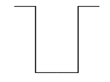
(a)

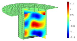
(b)

Figure 4: Result for example 1. (a) Cross section of the cavity. (b) Real part of the scattered electrical field $E_{x}$ at $k=10$ from a plane wave incidence.

We first consider a cavity with rectangular cross section (Fig. 4(a)). The depth and radius of the cavity are both set to $1$. We solve the test problem described above at several wavenumbers, with accuracy results shown in Table 1. Note that the CPU time is dominated by the computation of matrix elements, which scales quadratically with the number of unknowns. Because distinct Fourier modes are uncoupled, the solution of the various linear systems is embarassingly parallel and, for the problem sizes considered, does not dominate the cost despite the asymptotic $O(N_{pts}^{3})$ scaling. Note also that the accuracy is very high at low wavenumbers, and slowly deteriorates at higher wavenumber. The is due largely to the corner singularities in the density $\mathbf{M}$, which are stronger with increasing wavenumber. Additional additional refinement is necessary if higher accuracy were required. The scattering field for plane wave incidence at $k=10$ is given in Fig. 4(b) with 41 modes.

Results in Table 1 are obtained through solving eq. (2.23), without the low-frequency stabilization of eq. (4.13) for $k\geq 1$. In Fig. 5, we show the difference in using (2.23) or (4.13) as $k\rightarrow 0$. Low-frequency breakdown is clearly manifested in the original formulation, while (4.13) remains stable.

Figure 5: Illustration of low-frequency breakdown in the electric field. For Examples 1-3, the lower curve (red) shows the error of the solution obtained from (4.13) as a function of $k$ and the upper curve (blue) shows the error of the solution obtained from solving (2.23).

Example 2

For our second example, we consider the cavity whose generating curve (Fig. 6(a)) is given by

$$r(s) =[1-0.1\sin(6\pi s)]\sin(\frac{\pi}{2}s),$$ (6.3)

$$z(s) =-[1-0.1\sin(6\pi s)]\cos(\frac{\pi}{2}s),$$

for $s\in[0,1]$. The incoming field is again generated by the loop source as stated at the beginning of this section. Accuracy results are provided in Table 2 for various wavenumbers. A sufficient number of points is used to obtain high accuracy at all wavenumbers, with the computational cost again dominated by $T_{matgen}$. Fig. 6(b) shows the plane wave scattering at $k=10$ with 41 modes. We also compare the behavior of eqs. (2.23) and (4.13) in terms of low-frequency breakdown (Fig. 5) and see the advantages of (4.13) as $k\rightarrow 0$.

Table 2: Numerical results for the cavity of Example 2 at various wavenumbers.

$k$	$N_{f}$	$N_{pts}$	$N_{tot}$	$T_{matgen}(s)$	$T_{solve}(s)$	$E_{error}$
$1$	1	360	$960$	$112.0$	0.5	$4\cdot 10^{-15}$
$10$	1	360	$960$	$138.4$	0.5	$5\cdot 4^{-13}$
$10$	41	360	$960$	$273.4$	0.5	$5\cdot 10^{-13}$
$20$	1	720	$1920$	$578.8$	9.3	$4\cdot 10^{-12}$
$20$	61	720	$1920$	$1237.5$	12.3	$4\cdot 10^{-12}$
$40$	1	1440	$3840$	$4068.7$	134.5	$5\cdot 10^{-11}$
$40$	81	1440	$3840$	$9137.6$	145.1	$7\cdot 10^{-11}$

(a)

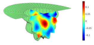
(b)

Figure 6: Results for Example 2. (a) Cross section of the cavity. (b) Real part of the scattered electric field $E_{x}$ at $k=10$ from a plane wave incidence.

Example 3

For our final example, we consider the cavity generated by a polygonal curve whose vertex coordinates are given by

$$V=\left\{(0,-0.5),\,(0.5,-0.5),\,(0.5,-0.7),\,(0.25,-0.7),\,(0.25,-1),\,(1,-1),\,(1,0)\right\},$$ (6.4)

see Figure 7(a).

We employ dyadic refinement on each segment to resolve the various corner singularities. Results are shown in Table 3, with accuracies given by comparison with the exact data. For plane wave incidence at $k=10$, Fig. 7(b) gives the scattered field. The low-frequency behavior is illustrated in Fig. 5, which shows the advantage of equation (4.13) again.

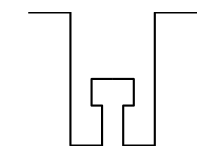
(a)

(b)

Figure 7: Results for Example 3. (a) Cross section of the cavity. (b) Real part of the scattered electrical field $E_{x}$ for $k=10$ from a plane wave incidence.

Table 3: Numerical results for the cavity of Example 3 at various wavenumbers.

$k$	$N_{f}$	$N_{pts}$	$N_{tot}$	$T_{matgen}(s)$	$T_{solve}(s)$	$E_{error}$
$1$	1	480	$1080$	$201.2$	0.70	$2\cdot 10^{-14}$
$10$	1	480	$1080$	$246.7$	0.70	$5\cdot 10^{-9}$
$10$	41	480	$1080$	$558.5$	0.75	$4\cdot 10^{-9}$
$20$	1	960	$2160$	$1217.8$	13.9	$6\cdot 10^{-7}$
$20$	41	960	$2160$	$2425.8$	13.2	$4\cdot 10^{-7}$
$40$	1	1920	$4320$	$5252.7$	119.6	$5\cdot 10^{-6}$

7 Conclusions

In this paper, we have developed a new integral representation for the problem of scattering from a three-dimensional cavity embedded in a perfectly conducting half-space which leads to a well conditioned integral equation. The resulting integral equation is resonance free for all wavenumbers $k$, immune from low-frequency (dense-mesh) breakdown, and we have established existence and uniqueness for its solution. In particular, the resulting linear system is well-conditioned all the way down to the static limit. Furthermore, the solution to this integral equation allows for the accurate reconstruction of the electric field in the limit as $k\to 0$. However, since inherently the unknowns in our formulation are current-like vector fields, reconstruction of the magnetic field suffers (albeit only mildly) from low-frequency breakdown. In order to overcome this, alternative representations using charge-like variables would have to be developed.

The effectiveness of the scheme was demonstrated in rotationally symmetric cavities using separation of variables in the azimuthal direction, and a subsequent high-order integral equation method on the cavity’s generating curve. The solution for each mode involves only line integrals along the generating curve that defines the geometry. This permits the use of efficient generalized Gaussian quadratures and stable, adaptive mesh refinement into the geometric singularities. We illustrated the performance of the scheme with several examples.

As discussed in section 4, one open question concerns a mild form of low-frequency breakdown in evaluating the magnetic field. We are presently investigating whether the use of generalized Debye sources [EG10, EG13] can be used to overcome this issue. Furthermore, in the present paper, we have made strong use of axisymmetry in developing a numerical solver. We are working on extending the relevant code to arbitrarily-shaped cavities using fully three-dimensional quadratures on triangulated surfaces.