Spin-$1$ Quasi-normal Frequencies in Schwarzschild space-time
for Large Overtone Number

Abstract

We analytically investigate the spin-$1$ quasinormal mode frequencies of Schwarzschild black hole space-time. We formally determine these frequencies to arbitrary order as an expansion for large imaginary part (i.e., large-$n$, where $n$ is the overtone number). As an example of the practicality of this formal procedure, we explicitly calculate the asymptotic behaviour of the frequencies up to order $n^{-5/2}$.

I Introduction

Quasinormal modes (QNMs) are damped modes of black holes possessing characteristic oscillation frequencies. For example, QNMs serve to describe the ‘ringdown’ stage of a gravitational waveform emitted by a perturbed black hole formed from the inspiral of two progenitor black holes, such as in the recent detection by the Laser Interferometer Gravitational-Wave Observatory Abbott et al. (2016). Matching an experimentally-observed waveform to an analytical prediction of the ‘ringdown’ based on QNMs may yield information of the main physical properties of the black hole, such as its mass and angular momentum. The QNMs in the ‘ringdown’ correspond to linear gravitational (spin-$2$) perturbations of the final black hole, but QNMs exist for linear field perturbations of any spin. In particular, electromagnetic (spin-$1$) perturbations are also of interest since the detection of electromagnetic waves from the host environment of the black hole inspiral might add useful information to that provided by the gravitational waves Schnittman (2011).

QNM frequencies are complex-valued, with the real part dictating the peak-to-peak frequency of the oscillation and the imaginary part its damping rate. The imaginary part of the frequencies, for a given multipole number $\ell$, are labelled by the overtone index $n\in\mathbb{N}$, with higher $n$ corresponding to larger imaginary part (in absolute value). Gravitational wave detectors are expected to be able to observe only the least-damped QNMs (i.e., the ones with small $n$). Various calulational techniques and results already exist for these low QNM frequencies for any spin of the field (see, e.g., Leaver (1985); Chandrasekhar and Detweiler (1975); QNM ). Highly-damped QNMs (i.e., the ones with large $n$) are interesting for other reasons. For example, Babb et al. (2011) have shown that QNMs in this large-$n$ limit probe the short length scale structure of a black hole space-time;  Keshet and Neitzke (2008) interpret them as semiclassical bound states along a specific contour in the complex-radius plane and speculate that they correspond to different sets of microscopic degrees of freedom. Asymptotics of QNM frequencies up to the first couple of orders for large-$n$ have been obtained in Motl and Neitzke (2003); Neitzke (2003); Maassen van den Brink (2004); Musiri and Siopsis (2003); Motl (2002); Musiri and Siopsis (2007); Casals and Ottewill (2012a) in Schwarzschild space-time (see Keshet and Neitzke (2008); Keshet and Hod (2007); Kao and Tomino (2008) in Kerr space-time).

In this paper we shall focus on spin-$1$ QNM frequencies of Schwarzschild space-time. These frequencies have the peculiarity that, for large imaginary part, they approach the imaginary axis (their real part decays like $n^{-3/2}$ – see Casals and Ottewill (2012a)); the real part of spin-$0$ and spin-$2$ frequencies, on the other hand, asymptote to a nonzero value. In Casals and Ottewill (2012a) we derived a large-$n$ expansion for the spin-$1$ QNM frequencies of Schwarzschild space-time up to $O\left(n^{-3/2}\right)$; the method in Casals and Ottewill (2012a) closely followed that in Maassen van den Brink (2004). In this paper we follow and extend this method in order to obtain a formal expansion of these frequencies up to arbitrary order for large-$n$. We prove the practicality of our formal expansion by giving the explicit expression of the frequencies up to two orders higher, $O\left(n^{-5/2}\right)$. We note that we presented this expansion in the Letter Casals and Ottewill (2012b). However, in this paper we describe in detail the derivation of these arbitrary-order results, we correct the term of $O\left(n^{-5/2}\right)$ given in Casals and Ottewill (2012b) and we give the general prescription for obtaining higher orders – e.g., in Eq.(43) we give the formal expansion of the QNM frequencies up to yet three orders higher, $O\left(n^{-4}\right)$.

We choose units $c=G=2M=1$, where $M$ is the mass of the Schwarzschild black hole.

II QuasiNormal Modes

The radial part of massless spin-$1$ field mode perturbations of Schwarzschild black hole space-time obeys the following equation Wheeler (1955); Ruffini et al. (1972):

$$\left\{\frac{d^{2}}{dr_{*}^{2}}+\omega^{2}-\left(1-\frac{1}{r}\right)\frac{\lambda}{r^{2}}\right\}\psi_{\ell}(r,\omega)=0.$$ (1)

In this equation, $\lambda\equiv\ell(\ell+1)$ where $\ell\in\mathbb{Z}^{+}$ is the multipole number, $\omega\in\mathbb{C}$ is the mode frequency (the time part of the mode behaving like $e^{-i\omega t}$), $r$ is the Schwarzschild radial coordinate and $r_{*}\equiv r+\ln(r-1)$.

We can define two linearly independent solutions, $f_{\ell}(r,\omega)$ and $g_{\ell}(r,\omega)$, of Eq.(1) defined by the boundary conditions (see later for when these are meaningful):

$$f_{\ell}\sim e^{-i\omega r_{*}},\quad r_{*}\to-\infty,$$ (2)

$$f_{\ell}\sim A^{out}_{\ell}e^{+i\omega r_{*}}+A^{in}_{\ell}e^{-i\omega r_{*}},\quad r_{*}\to+\infty,$$ (3)

and

$$g_{\ell}\sim e^{+i\omega r_{*}},\quad r_{*}\to+\infty,$$ (4)

where $A^{out}_{\ell}=A^{out}_{\ell}(\omega)$ and $A^{in}_{\ell}=A^{in}_{\ell}(\omega)$ are, respectively, reflection and incidence coefficients. The Wronskian of these two solutions is

$$W\left(\omega\right)\equiv W[g_{\ell},f_{\ell};\omega]=f_{\ell}\frac{dg_{\ell}}{dr_{*}}-g_{\ell}\frac{df_{\ell}}{dr_{*}}=2i\omega A^{in}_{\ell}.$$ (5)

QNM frequencies are the roots in the complex-frequency plane of $W\left(\omega\right)=0$. Physically, they correspond to waves which are purely-ingoing into the horizon and purely outgoing to radial infinity. Mathematically, they correspond to poles of the Fourier modes of the retarded Green function of Eq.(1). In Schwarzschild space-time, the real part of the QNM frequencies (for any spin of the field) increases with $\ell$ and the magnitude of their imaginary part increases with the so-called overtone number $n=0,1,2\dots$. The imaginary part is negative, and therefore the QNMs decay with time, at a faster rate the larger $n$ is.

We note that the radial solution $g_{\ell}$ possesses a branch point at $\omega=0$ Leaver (1986); Casals and Ottewill (2013, 2015). We shall take the branch cut emanating from it to lie along the negative imaginary axis on the complex-$\omega$ plane. This branch cut is inherited by the Wronskian via Eq.(5). We shall denote by $g_{\ell+}$ the limiting value of $g_{\ell}$ onto the branch cut as coming from the 4th quadrant.

III Method

We follow the method that we used in Casals and Ottewill (2012a) and which is based on Maassen van den Brink (2000). In Casals and Ottewill (2012a) we derived the large-$n$ expansion for the spin-$1$ QNM frequencies to leading order in the real part. In this section we describe the method while in the next section we focus on the modifications to Casals and Ottewill (2012a) needed in order to obtain the expansion to arbitrary order in $n$.

The boundary condition in Eq.(2) or (4) becomes meaningless when the given asymptotic solution becomes subdominant with respect to another linearly independent asymptotic solution. Specifically, in order for these conditions to determine the solutions uniquely they must be imposed in the regions $\text{Re}\left(-i\omega r_{*}\right)\leq 0$ for $f_{\ell}$ and $\text{Re}\left(i\omega r_{*}\right)\leq 0$ for $g_{\ell}$. The solutions are then defined elsewhere in the complex-$\omega$ and complex$-r_{*}$ planes by analytic continuation.

Eq.(1) admits two linearly-independent asymptotic expansions for large $\left|\omega\right|$ which, to leading order, are: $g_{a}(r,\mp i\sigma)\sim e^{\pm\sigma r_{*}}$, where $\sigma\equiv i\omega$. Since we are interested in an expansion for large-$n$ (and fixed $\ell$), that is an expansion for $\sigma$ “near” the positive real line, the curves along which neither of these two asymptotic solutions dominates over the other one correspond to “near” $\text{Re}\left(r_{*}\right)=0$ These curves in the complex-$r$ plane are the so-called anti-Stokes lines. These asymptotic expansions are valid away from the regular singular points $r=0$ (specifically, for $|r\sqrt{\sigma}|\gg 1$) and $1$ of the ordinary differential equation (1) and away from the anti-Stokes lines. Fig.1 illustrates the anti-Stokes lines as well as the contours that we follow in order to obtain the desired asymptotics for $f_{\ell}$ and $g_{\ell}$. We describe these contours in the following two paragraphs.

For $g_{\ell}$, the boundary condition Eq.(4) can be imposed, by analytic continuation, on $|r|\to\infty$ (instead of $r\to\infty$) along an anti-Stokes line going to infinity; in the case of $g_{\ell+}$, that is the line going along the upper $r$-plane (this region is exemplified by the point A in Fig.1(a)). Therefore, $g_{\ell+}(r,-i\sigma)\sim g_{a}(r,-i\sigma)$ there. We can analytically continue that solution along the anti-Stokes line down to a region ‘near’ $r=0$ (exemplified by a point B). There, we match our asymptotic expression for $g_{\ell}$ to a linear combination of two linearly-independent functions $\psi_{i}$, $i=1,2$, which are asymptotic solutions for large $\sigma$ with fixed $r\sqrt{\sigma}$. These new solutions are given in terms of special functions which we know how to analytically continue from the anti-Stokes line with $\arg(r)=3\pi/4$ to the one with $\arg(r)=\pi/4$. The resulting expression for $g_{\ell+}$ there can then be matched to a new linear combination of $g_{a}(r,\mp i\sigma)$. Finally, that linear combination can be analytically continued along the anti-Stokes line all the way to $r_{*}=0$ (point C).

As for $f_{\ell}$, we can also asymptotically express it as a linear combination of $g_{a}(r,\mp i\sigma)$ at a point $r\gtrsim 1$ with $r_{*}<0$ (point D in Fig.1(b)). The boundary condition Eq.(2) tells us that the coefficient of the dominant solution there (i.e., $g_{a}(r,+i\sigma)$) in this combination is equal to $1$; the coefficient of the subdominant solution there (i.e., of $g_{a}(r,-i\sigma)$) is the quantity that we wish to determine. We can continue this combination to $r_{*}=0$ (point C) and then anticlockwise along the anti-Stokes line up to $\arg(r)=\pi/4$. We there match it to a linear combination of $\psi_{i}$, which we can analytically continue on to the anti-Stokes line on $\arg(r)=-\pi/4$. There we can match it to a new linear combination of $g_{a}(r,\mp i\sigma)$, which we can continue anticlockwise along the anti-Stokes line finally back to $r_{*}=0$. This yields a formal expression for the monodromy of $f_{\ell}$ around $r=1$, which can be compared with the exact monodromy that straight-forwardly follows from Eq.(2):

$$f_{\ell}\left((r-1)e^{2\pi i},-i\sigma\right)=e^{-2\pi i\sigma}f_{\ell}\left(r-1,-i\sigma\right).$$ (6)

This comparison then yields the previously undetermined coefficient of $g_{a}(r,-i\sigma)$ in the expression of $f_{\ell}$ in terms of $g_{a}(r,\mp i\sigma)$ at $r_{*}=0$.

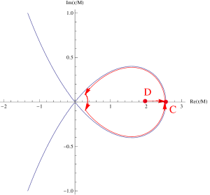
Figure 1: Schematic illustration on the complex-$r$ plane in Schwarzschild when $\sigma=i\omega>0$ of anti-Stokes lines (i.e., where $\text{Re}(r_{*})=0$; curves in blue) and of the contours (curves in red) that we follow in order to calculate the large-$\sigma$ asymptotics of the radial solutions $g_{\ell+}$ (top) and $f_{\ell}$ (bottom).

IV Radial Solutions

We proceed to find two convenient sets of two linearly independent asymptotic solutions of Eq.(1) which are valid in different regimes, but which have a common regime of validity. The first set is a WKB expansion which is valid for large-$|\omega|$ and away from the singular points $r=0$ (specifically, $|r\sqrt{\sigma}|\gg 1$ is required), $1$ and away from the anti-Stokes lines:

$$g_{a}(r,\pm i\sigma)\equiv e^{\mp\sigma r_{*}}\sum_{k=0}^{\infty}\frac{g_{k}(r)}{\sigma^{k}},\quad g_{0}(r)=1,$$ (7)

for some functions $g_{k}(r)$, $k>1$ (we will not need the $g_{k}$ explicitly in order to find the QNMs). We note that neither expansion $g_{a}(r,\pm i\sigma)$ dominates over the other along an anti-Stokes line; $g_{a}(r,-i\sigma)$ dominates over $g_{a}(r,+i\sigma)$ inside the oval-shaped region in Fig.1 (which contains $r=1$), and then, every time an anti-Stokes line is crossed the dominant and subdominant WKB expansions are swopped. All $k$-sums from now on will be assumed to run from $0$ to $\infty$ except where otherwise indicated. By comparing Eqs.(4) and (7), it follows that

$$g_{\ell+}(r,-i\sigma)\sim g_{a}(r,-i\sigma),\quad\sigma\gg 1,\ |\arg(r)-\pi|<3\pi/4,$$ (8)

where we are only neglecting exponentially small corrections.

Following Maassen van den Brink (2004); Casals and Ottewill (2012a), we define $v\equiv r^{2}\sigma/2$ and then write Eq. (1) as

$$\left(\psi_{\ell}^{\prime\prime}-\psi_{\ell}\right)-\frac{1}{\sqrt{\sigma}}\frac{1}{(2v)^{3/2}}\mathcal{D}_{1}\psi_{\ell}+\frac{1}{\sigma}\frac{1}{2v}\mathcal{D}_{2}\psi_{\ell}=0,$$ (9)

where a prime denotes a derivative with respect to $v$ and

$$\mathcal{D}_{1} \equiv 8D^{2}-6D-\lambda,$$ (10)

$$\mathcal{D}_{2} \equiv 4D^{2}-2D-\lambda,$$ (11)

with $D\equiv v\tfrac{d}{dv}$.

Again following Maassen van den Brink (2004); Casals and Ottewill (2012a), we now write $g_{a}(r,\pm i\sigma)e^{\pm i\pi\sigma}e^{\mp v}$ as a power series in $\dfrac{v^{1/2}}{\sigma^{b}}$ with $b\geq 1/6$, and we obtain, for $\arg(r-1)\in(0,\pi]$:

$$g_{a}(r,\pm i\sigma)\sim e^{\mp i\pi\sigma}e^{\pm v}\left(\sum_{k}(\mp 1)^{k}\frac{d_{k}}{\sigma^{k}}+\dots\right),\quad d_{0}=1,$$ (12)

for some coefficients $d_{k}$ for $k>1$ (again, we will not need the $d_{k}$ explicitly in order to find the QNMs). The dots in Eq.(12) only involve terms which, when replacing $\sigma$ by $\mu\,v^{3}$, go to zero in the double limit $v,\mu\to\infty$.

We may now find a second set of asymptotic solutions of Eq.(9) valid for fixed $v$ as expansions in powers of $\sigma^{-1/2}$ as

$$\psi_{i}(v)\equiv\sum_{k=0}^{\infty}\psi_{i}^{(k)}(v),\quad i=1,2,$$ (13)

starting with two independent solutions of the limiting $\sigma\to\infty$ equation:

$$\psi_{1}^{(0)}(v)=\frac{2}{\sigma}\sinh v,\quad\psi_{2}^{(0)}(v)=\cosh v.$$ (14)

The functions $\psi_{i}^{(k)}(v)$, $\forall k>0$, may be obtained in the following way. Formally (see explanation below), matching powers of $\sigma^{-1/2}$ in Eq. (1) we obtain a sequence of coupled integral equations for the $\psi_{i}^{(k)}$ employing the $0^{\mathrm{th}}$-order Green function as

$$\psi_{i}^{(k)}(v)=$$

$$\ \sinh v\!\!\int_{0}^{v}\!du\cosh u\left\{\frac{\mathcal{D}_{1}\psi_{i}^{(k-1)}(u)}{\sqrt{\sigma}\ (2u)^{3/2}}-\frac{\mathcal{D}_{2}\psi_{i}^{(k-2)}(u)}{\sigma\ (2u)}\right\}$$

$$\ -\cosh v\!\!\int_{0}^{v}\!du\sinh u\left\{\frac{\mathcal{D}_{1}\psi_{i}^{(k-1)}(u)}{\sqrt{\sigma}\ (2u)^{3/2}}-\frac{\mathcal{D}_{2}\psi_{i}^{(k-2)}(u)}{\sigma\ (2u)}\right\},$$

$$\forall k>0,\quad i=1,2,$$ (15)

with the understanding that $\psi_{1}^{(-1)}(u)=\psi_{2}^{(-1)}(u)\equiv 0$ and that the operators $\mathcal{D}_{1,2}$ in Eq.(IV) are with respect to $u$ instead of $v$.

To understand the reason we say ‘formally’ above becomes clearer if we note that $\mathcal{D}_{1}\psi_{1}^{(0)}(u)=O(u)$ and $\mathcal{D}_{1}\psi_{2}^{(0)}(u)=-\lambda+O(u^{2})=-\lambda\cosh u+O(u^{2})$ as $u\to 0$. Thus, while both integrals in Eq.(IV) exist for $\psi_{1}^{(0)}$, the first integral is divergent for $\psi_{2}^{(0)}$. We may regularise it by adding an (infinite) multiple of our original solution, $\psi_{1}^{(0)}(v)=\frac{2}{\sigma}\sinh v$. To do so, we rewrite the problematic term

$$\int_{0}^{v}\!du\frac{\cosh u}{(2u)^{3/2}}\left(-\lambda\cosh u\right)$$

$$\qquad=\int_{0}^{v}\!du\frac{1}{(2u)^{3/2}}\left(-\lambda\cosh^{2}u+\lambda\right)-\int_{0}^{v}\!du\frac{1}{(2u)^{3/2}}\lambda$$

$$\qquad=\int_{0}^{v}\!du\frac{1}{(2u)^{3/2}}\left(-\lambda\sinh^{2}u\right)+\frac{\lambda}{(2v)^{1/2}},$$ (16)

where in the last line we have dropped our infinite constant, corresponding to the multiple of $\psi_{1}^{(0)}$. With this adjustment it is straightforward to find

$$\psi_{1}^{(1)}(v) =\frac{4\sqrt{2}}{3\sigma^{3/2}}v^{3/2}\cosh v+\frac{\lambda\sqrt{\pi}}{2\sigma^{3/2}}\left(e^{-v}\operatorname{erfi}\left(\sqrt{2v}\right)-e^{v}\operatorname{erf}\left(\sqrt{2v}\right)\right),$$

$$\psi_{2}^{(1)}(v) =\frac{2\sqrt{2}}{3\sigma^{1/2}}v^{3/2}\sinh v+\frac{\lambda\sqrt{\pi}}{4\sigma^{1/2}}\left(e^{-v}\operatorname{erfi}\left(\sqrt{2v}\right)+e^{v}\operatorname{erf}\left(\sqrt{2v}\right)\right),$$ (17)

where we use the standard definitions of the entire functions

$$\operatorname{erf}(z)=\frac{2}{\sqrt{\pi}}\int_{0}^{z}\!du\>e^{-u^{2}}$$ (18)

and $\operatorname{erfi}(z)=\operatorname{erf}(iz)/i$. From these definitions it follows that

$$\operatorname{erf}(\sqrt{2e^{i\pi}v}) =i\operatorname{erfi}(\sqrt{2v}),$$ (19)

$$\operatorname{erfi}(\sqrt{2e^{i\pi}v}) =i\operatorname{erf}(\sqrt{2v}).$$

Correspondingly, it is straightforward to check that

$$\psi_{1}^{(k)}(e^{i\pi}v) =-e^{i\pi k/2}\psi_{1}^{(k)}(v),\ k=0,1,$$

$$\psi_{2}^{(k)}(e^{i\pi}v) =e^{i\pi k/2}\psi_{2}^{(k)}(v),\ k=0,1.$$

It is easy to also derive this behaviour from the formal expression Eq.(IV) but we will see below that at higher order this is broken by the regularisation procedure and anomalous terms arise.

To determine the regularisation required at second order, we first note that $\mathcal{D}_{1}\psi_{1}^{(1)}(u)=O(u^{3/2})$ and $\mathcal{D}_{2}\psi_{1}^{(0)}(u)=O(u^{1/2})$ as $u\to 0$, so both integrals in Eq.(IV) are well-defined. However, $\mathcal{D}_{1}\psi_{2}^{(1)}(u)=-\lambda(1+\lambda)\sqrt{\dfrac{2u}{\sigma}}+O(u^{5/2})$ and $\mathcal{D}_{1}\psi_{2}^{(0)}(u)=-\lambda+O(u^{2})$ as $u\to 0$, and so the corresponding terms must again be adjusted by

$$\int_{0}^{v}\!du\cosh u\left\{\frac{\mathcal{D}_{1}\psi_{2}^{(1)}(u)}{\sqrt{\sigma}\ (2u)^{3/2}}-\frac{\mathcal{D}_{2}\psi_{2}^{(0)}(u)}{\sigma\ (2u)}\right\}$$

$$\ =\int_{0}^{v}\!du\left\{\frac{\cosh u\mathcal{D}_{1}\psi_{2}^{(1)}(u)}{\sqrt{\sigma}\ (2u)^{3/2}}+\frac{\lambda(1+\lambda)}{\sigma\ (2u)}\right\}$$

$$\ \ -\ \int_{0}^{v}\!du\left\{\frac{\cosh u\mathcal{D}_{2}\psi_{2}^{(0)}(u)}{\sigma\ (2u)}+\frac{\lambda}{\sigma\ (2u)}\right\}-\frac{\lambda^{2}}{2\sigma}\ln v,$$

where again we have just dropped an infinite constant which simply multiplies $\psi_{1}^{(0)}(e^{i\pi}v)$. With this regularization, we find, using Eqs.(IV), (14) and (17), that

$$\psi_{1}^{(2)}(v) =\frac{2}{9\sigma^{2}}v^{2}(4v\sinh v+9\cosh v)+\frac{\lambda}{3\sigma^{2}}\Bigl{[}4v\sinh v-\sqrt{2\pi}v^{3/2}\bigl{(}e^{v}\operatorname{erf}(\sqrt{2v})+e^{-v}\operatorname{erfi}(\sqrt{2v})\bigr{)}\Bigr{]}$$

$$-\frac{\lambda^{2}}{4\sigma^{2}}\Bigl{[}e^{v}\bigl{(}\Gamma(0,2v)+\log(2v)+\gamma_{E}\bigr{)}+e^{-v}\bigl{(}\Gamma(0,-2v)+\log(-2v)+\gamma_{E}\bigr{)}$$

$$\quad-4e^{-v}v\,_{2}F_{2}\left(1,1;\tfrac{3}{2},2;-2v\right)+4e^{v}v\,_{2}F_{2}\left(1,1;\tfrac{3}{2},2;2v\right)-2\pi\operatorname{erf}(\sqrt{2v})\operatorname{erfi}(\sqrt{2v})\sinh v\Bigr{]},$$

$$\psi_{2}^{(2)}(v) =\frac{1}{9\sigma}v^{2}(4v\cosh v+9\sinh v)+\frac{\lambda}{6\sigma}\Bigl{[}4(v\cosh v-\sinh v)+\sqrt{2\pi}v^{3/2}\bigl{(}e^{v}\operatorname{erf}(\sqrt{2v})-e^{-v}\operatorname{erfi}(\sqrt{2v})\bigr{)}\Bigr{]}$$

$$-\frac{\lambda^{2}}{8\sigma}\Bigl{[}4\log v\sinh v+8\sinh v-e^{v}\bigl{(}\Gamma(0,2v)+\log(2v)+\gamma_{E}\bigr{)}+e^{-v}\bigl{(}\Gamma(0,-2v)+\log(-2v)+\gamma_{E}\bigr{)}$$

$$\quad+4e^{-v}v\,_{2}F_{2}\left(1,1;\tfrac{3}{2},2;-2v\right)+4e^{v}v\,_{2}F_{2}\left(1,1;\tfrac{3}{2},2;2v\right)-2\pi\operatorname{erf}(\sqrt{2v})\operatorname{erfi}(\sqrt{2v})\cosh v\Bigr{]},$$ (20)

where $\gamma_{E}$ is Euler’s constant, $\Gamma(0,\pm 2v)$ is the incomplete gamma function and $\,{}_{2}F_{2}$ is a generalized hypergeometric function. We note that $\Gamma(0,z)+\log(z)+\gamma_{E}$ is an entire function of $z$ Erdelyi et al. (1953). We also obtain, from Eqs.(IV), (17) and (20), without any regularization required:

$$\psi_{1}^{(3)}(v)=\frac{4\sqrt{2}}{405\sigma^{5/2}}v^{5/2}\Bigl{[}2\left(10v^{2}+81\right)\cosh v+135v\sinh v\Bigr{]}$$

$$+\frac{\lambda}{144\sigma^{5/2}}\Bigl{[}-\sqrt{\pi}(32v^{3}+72v^{2}+3)e^{v}\operatorname{erf}(\sqrt{2v})+\sqrt{\pi}(32v^{3}-72v^{2}-3)e^{-v}\operatorname{erfi}(\sqrt{2v})+4\sqrt{2v}(28v\sinh v+3\cosh v)\Bigr{]}$$

$$+\frac{\lambda^{2}}{24\sigma^{5/2}}\Bigl{[}-16\sqrt{2}v^{5/2}\bigl{[}e^{-v}\,_{2}F_{2}(1,1;\tfrac{3}{2},2;-2v)-e^{v}\,_{2}F_{2}(1,1;\tfrac{3}{2},2;2v)\bigr{]}$$

$$\ +\frac{8}{3}\sqrt{2}v^{3/2}\left(e^{v}\,_{2}F_{2}(\tfrac{3}{2},\tfrac{3}{2};\tfrac{5}{2},\tfrac{5}{2};-2v)-e^{-v}\,_{2}F_{2}(\tfrac{3}{2},\tfrac{3}{2};\tfrac{5}{2},\tfrac{5}{2};2v)\right)-6\sqrt{2v}\left(e^{v}\,_{2}F_{2}(\tfrac{1}{2},\tfrac{1}{2};\tfrac{3}{2},\tfrac{3}{2};-2v)-e^{-v}\,_{2}F_{2}(\tfrac{1}{2},\tfrac{1}{2};\tfrac{3}{2},\tfrac{3}{2};2v)\right)$$

$$\ +8\sqrt{2}\pi v^{3/2}\operatorname{erf}(\sqrt{2v})\operatorname{erfi}(\sqrt{2v})\cosh v+\sqrt{\pi}e^{v}(3-8v)\operatorname{erf}(\sqrt{2v})+\sqrt{\pi}e^{-v}(8v+3)\operatorname{erfi}(\sqrt{2v})$$

$$\ +4\sqrt{2}v^{3/2}\bigl{[}e^{-v}(\Gamma(0,-2v)+\log(-2v)+\gamma_{E})-e^{v}(\Gamma(0,2v)+\log(2v)+\gamma_{E})\bigr{]}\Bigr{]}$$

$$+\frac{\lambda^{3}}{16\sigma^{5/2}}\Bigl{[}-8\sqrt{\pi}v\bigl{[}e^{v}\operatorname{erf}(\sqrt{2v})\,_{2}F_{2}(1,1;\tfrac{3}{2},2;-2v)+e^{-v}\operatorname{erfi}(\sqrt{2v})\,_{2}F_{2}(1,1;\tfrac{3}{2},2;2v)\bigr{]}$$

$$\ +16\sqrt{2v}\left(e^{v}\,_{2}F_{2}\left(\tfrac{1}{2},\tfrac{1}{2};\tfrac{3}{2},\tfrac{3}{2};-2v\right)+e^{-v}\,_{2}F_{2}\left(\tfrac{1}{2},\tfrac{1}{2};\tfrac{3}{2},\tfrac{3}{2};2v\right)\right)-16\sqrt{2v}\cosh v\left(\,{}_{2}F_{2}\left(\tfrac{1}{2},1;\tfrac{3}{2},\tfrac{3}{2};-2v\right)+\,_{2}F_{2}\left(\tfrac{1}{2},1;\tfrac{3}{2},\tfrac{3}{2};2v\right)\right)$$

$$\ -2\sqrt{\pi}e^{v}\operatorname{erf}(\sqrt{2v})(\Gamma(0,-2v)+\log(-2v)+\gamma_{E})-2\sqrt{\pi}e^{-v}\operatorname{erfi}(\sqrt{2v})(\Gamma(0,2v)+\log(2v)+\gamma_{E})\Bigr{]}-\frac{\lambda^{3}\pi}{\sqrt{2}\sigma^{5/2}}\psi_{1R}^{\ (3)}(v),$$ (21)

where

$$\psi_{1R}^{\ (3)}(v)\equiv\int\limits_{0}^{v}\frac{\operatorname{erf}(\sqrt{2u})\operatorname{erfi}(\sqrt{2u})\sinh(v-2u)}{\sqrt{u}}\>\text{d}u.$$

From the expressions in Eqs.(14) and (20) together with Eq.(19), it is easy to check that

$$\psi_{1}^{(k)}(e^{i\pi}v)=-e^{i\pi k/2}\psi_{1}^{(k)}(v),\ k=2,$$ (22)

$$\psi_{2}^{(k)}(e^{i\pi}v)=e^{i\pi k/2}\left[\psi_{2}^{(k)}(v)-\frac{i\pi\lambda^{2}}{4}\psi_{1}^{(k-2)}(v)\right],\ k=2.$$ (23)

Furthermore, an examination of the small-$u$ behaviour of the factors in the integrand in Eq.(IV) for $\psi_{2}^{(3)}(v)$ yields: $\mathcal{D}_{2}\psi_{2}^{(2)}(u)=O(u\ln u)$ and $\mathcal{D}_{1}\psi_{2}^{(1)}(u)=O(u^{1/2})$ as $u\to 0$. Therefore, no regularisation is required in the calculation of $\psi_{2}^{(3)}(v)$. Indeed, it follows from the smoothing properties of the integral expression in Eq.(IV), that no additional regularisation is required beyond order $k=2$. It then follows from Eqs.(IV), (22) and (23) that

$$\psi_{1}^{(k)}(e^{i\pi}v)=-e^{i\pi k/2}\psi_{1}^{(k)}(v),\ \forall k\geq 0,$$ (24)

$$\psi_{2}^{(k)}(e^{i\pi}v)=e^{i\pi k/2}\left[\psi_{2}^{(k)}(v)-\frac{i\pi\lambda^{2}}{4}\psi_{1}^{(k-2)}(v)\right],\ \forall k\geq 2.$$ (25)

In addition, by a similar argument, we have that, along $\arg(r)=\pi/4$,

$$e^{-i\pi(k-2)/4}\psi_{1}^{(k)}(v)\in\mathbb{R},$$ (26)

$$e^{-i\pi k/4}\left[\psi_{2}^{(k)}(v)+\frac{i\pi\lambda^{2}}{8}\psi_{1}^{(k-2)}(v)\right]\in\mathbb{R}.$$

From Eq.(26) it follows that, along $\arg(r)=\pi/4$ ($\arg(v)=\pi/2$),

$$\tilde{\psi}_{i}=A_{i}e^{v}+B_{i}e^{-v},$$ (27)

$$A_{1}\equiv{\sum_{k}}\frac{\alpha_{k}}{\sigma^{k/2}},\quad A_{2}\equiv{\sum_{k}}\frac{\beta_{k}-i\alpha_{1}^{2}\alpha_{k-2}}{\sigma^{k/2}},$$

$$B_{1}\equiv-{\sum_{k}}\frac{i^{k}\alpha_{k}^{*}}{\sigma^{k/2}},\quad B_{2}\equiv{\sum_{k}}\frac{i^{k}\left(\beta_{k}^{*}-i\alpha_{1}^{2}\alpha_{k-2}^{*}\right)}{\sigma^{k/2}},$$

for some constants $\alpha_{k}$ and $\beta_{k}$, where $\tilde{\psi}_{1}\equiv\sigma\psi_{1}$ and $\tilde{\psi}_{2}\equiv 2\psi_{2}$, and where in the expansions of $A_{1,2}$ and of $B_{1,2}$ we have dropped any terms which vanish in the double limit described below Eq.(12).

We can determine the values of $\alpha_{k}$, $k=0\to 3$, directly from the expressions for $\tilde{\psi}_{1}^{(k)}$, $k=0\to 3$, in Eqs.(14), (17), (20) and (21), by directly carrying out the double asymptotic limit described below Eq.(12) along $\arg(v)=\pi/2$. Apart from $\psi_{1R}^{\ (3)}(v)$, all terms above are given in terms of standard functions so that we may obtain the asymptotic expansions along $v=ix$ as $x\to\infty$ from reference texts such as DLMF DLMF . For $\psi_{1R}^{\ (3)}(ix)$ we write

$$\psi_{1R}^{\ (3)}(ix)=$$

$$\frac{e^{i\pi/4}}{4\sqrt{\pi}}\Bigl{[}\cos x\Bigl{(}4+\pi-2\log 2-8C\left(2\sqrt{\tfrac{x}{\pi}}\right)-4\pi S\left(2\sqrt{\tfrac{x}{\pi}}\right)-2\pi C\left(2\sqrt{\tfrac{x}{\pi}}\right)^{2}+4\pi C\left(2\sqrt{\tfrac{x}{\pi}}\right)S\left(2\sqrt{\tfrac{x}{\pi}}\right)+2\pi S\left(2\sqrt{\tfrac{x}{\pi}}\right)^{2}$$

$$\qquad\qquad\qquad\qquad+4\sqrt{2}x\left(e^{i\pi/4}\,_{2}F_{2}\left(1,1;\tfrac{3}{2},2;-2ix\right)+e^{-i\pi/4}\,_{2}F_{2}\left(1,1;\tfrac{3}{2},2;2ix\right)\right)\Bigr{)}+$$

$$\sin x\Bigl{(}4-\pi-2\log 2+\frac{4}{\sqrt{\pi}\sqrt{x}}-8S\left(2\sqrt{\tfrac{x}{\pi}}\right)+4\pi C\left(2\sqrt{\tfrac{x}{\pi}}\right)-2\pi C\left(2\sqrt{\tfrac{x}{\pi}}\right)^{2}-4\pi C\left(2\sqrt{\tfrac{x}{\pi}}\right)S\left(2\sqrt{\tfrac{x}{\pi}}\right)+2\pi S\left(2\sqrt{\tfrac{x}{\pi}}\right)^{2}$$

$$\qquad\qquad\qquad\qquad-4\sqrt{2}x\left(e^{-i\pi/4}\,_{2}F_{2}\left(1,1;\tfrac{3}{2},2;-2ix\right)+e^{i\pi/4}\,_{2}F_{2}\left(1,1;\tfrac{3}{2},2;2ix\right)\right)\Bigr{)}\Bigr{]}+\psi_{1\text{rem}}^{\ (3)}(x),$$

where

$$\psi_{1\text{rem}}^{\ (3)}(x) \equiv-e^{i\pi/4}\int\limits_{x}^{\infty}\sin(x-2u)\Bigr{[}\frac{\operatorname{erfc}\bigl{(}(1+i)\sqrt{u}\bigr{)}\operatorname{erfc}\bigl{(}(1-i)\sqrt{u}\bigr{)}}{\sqrt{u}}-\frac{1}{2\pi}\frac{1}{u^{3/2}}\Bigl{]}\>\text{d}u,$$

and $C(z)$ and $S(z)$ are Fresnel integrals:

$$C(z)\equiv\int_{0}^{z}dt\cos\left(\frac{\pi t^{2}}{2}\right),\quad S(z)\equiv\int_{0}^{z}dt\sin\left(\frac{\pi t^{2}}{2}\right).$$

We do not have a closed-form expression for $\psi_{1\text{rem}}^{\ (3)}(x)$ but all that matters is that it can readily be shown to vanish as $x\to\infty$ and so does not contribute to $\alpha_{3}$. The results we obtain for $\alpha_{k}$, $k=0\to 3$, in this manner are:

$$\alpha_{0}=1,$$ (28)

$$\alpha_{1}=-\frac{\lambda\sqrt{\pi}}{2},$$

$$\alpha_{2}=\frac{\lambda^{2}\ln 2}{2}-\frac{\lambda}{12},$$

$$\alpha_{3}=\frac{\lambda^{3}\sqrt{\pi}}{8}(4\ln 2-\pi)+\frac{\lambda^{2}\sqrt{\pi}}{24}-\frac{\lambda\sqrt{\pi}}{48}.$$

From Eqs.(27) and (24) it follows that along $\arg(r)=3\pi/4$ (i.e., $\arg(v)=3\pi/2$),

$$\tilde{\psi}_{i}=C_{i}e^{v}+D_{i}e^{-v}$$ (29)

$$C_{1}\equiv{\sum_{k}}\frac{(-1)^{k}\alpha_{k}^{*}}{\sigma^{k/2}},\quad C_{2}\equiv{\sum_{k}}\frac{(-1)^{k}\left(\beta_{k}^{*}-3i\alpha_{1}^{2}\alpha_{k-2}\right)}{\sigma^{k/2}}$$

$$D_{1}\equiv-{\sum_{k}}\frac{i^{k}\alpha_{k}}{\sigma^{k/2}},\quad D_{2}\equiv{\sum_{k}}\frac{i^{k}\left(\beta_{k}-3i\alpha_{1}^{2}\alpha_{k-2}\right)}{\sigma^{k/2}}.$$

We now equate Eqs.(27) and (29) in the sector $\arg(r)\in(\pi/4,3\pi/4)$. Equating the dominant terms in that sector, i.e., $B_{1}=D_{1}$ and $B_{2}=D_{2}$, respectively yields $\alpha_{k}\in\mathbb{R}$ and $\text{Im}\beta_{k}=\alpha_{1}^{2}\alpha_{k-2}$. Therefore, $A_{1},A_{2}\in\mathbb{R}$. From the subdominant terms in that sector it follows that

$$A_{1}B_{2}-B_{1}A_{2}=C_{1}B_{2}-C_{2}B_{1}.$$ (30)

This constraint explicitly reads

$$\sum_{m=0}^{k}\alpha_{m}i^{m}\left\{\text{Re}\beta_{k-m}\left[i^{k}\left((-1)^{m}-1\right)-(-1)^{k+m}+1\right]-\right.$$

$$\ \left.2i\alpha_{1}^{2}\alpha_{k-m-2}\left[i^{k}\left((-1)^{m}-1\right)-2(-1)^{k+m}\right]\right\}=0,$$

$$\forall k=1,2,\dots,$$ (31)

with $\alpha_{-2}\equiv\alpha_{-1}\equiv 0$. This yields, for example, $\text{Re}\beta_{1}=-\alpha_{1}$ and $\text{Re}\beta_{3}=-\alpha_{3}+2\alpha_{1}^{3}-\alpha_{1}\alpha_{2}+\alpha_{1}\text{Re}\beta_{2}$. Indeed, these constraints serve to determine $\text{Re}\beta_{k}$ except when $k=4r-2$ for $r\in\mathbb{N}$; those terms are undetermined corresponding to the fact that Eq.(IV) yields a trivial equation when $k=4r$. These terms, however, do not contribute to the QNM condition.

We now have two sets of solutions, $\{g_{a}(r,\pm i\sigma)\}$ of Eq.(12) and $\{\tilde{\psi}_{i},i=1,2\}$ of Eq.(29), which are both valid on a common region: along $\arg(r)=3\pi/4$ and for $v\gg 1$ and $v^{3}/\sigma\ll 1$. We now proceed to match them in this region. Inverting the relationships Eq.(29) we readily have that, along $\arg(r)=3\pi/4$,

$$e^{v} =\frac{D_{2}\tilde{\psi}_{1}-D_{1}\tilde{\psi}_{2}}{W_{C}},$$ (32)

$$e^{-v} =\frac{C_{1}\tilde{\psi}_{2}-C_{2}\tilde{\psi}_{1}}{W_{C}},$$

where $W_{C}\equiv C_{1}D_{2}-D_{1}C_{2}$. Inserting these in Eq.(12) allows us to express $g_{a}$ in terms of $\tilde{\psi}_{i}$ along $\arg(r)=3\pi/4$:

$$e^{+i\pi\sigma}g_{a}(r,i\sigma) =\frac{\left(D_{2}\tilde{\psi}_{1}-D_{1}\tilde{\psi}_{2}\right)}{W_{C}}\sum_{k}(-1)^{k}\frac{d_{k}}{\sigma^{k}},$$ (33)

$$e^{-i\pi\sigma}g_{a}(r,-i\sigma) =\frac{\left(C_{1}\tilde{\psi}_{2}-C_{2}\tilde{\psi}_{1}\right)}{W_{C}}\sum_{k}\frac{d_{k}}{\sigma^{k}}.$$ (34)

From Eq.(8), we have that $g_{\ell+}$ is asymptotically given by the right hand side of Eq.(34). Although such expression for $g_{\ell+}$ in terms of $\tilde{\psi}_{i}$ was derived specifically along $\arg(r)=3\pi/4$, it is valid $\forall\arg(r)$ by analytic continuation. In particular, it is valid along $\arg(r)=\pi/4$, where we can use Eq.(27) together with Eq.(12) in order to obtain $g_{\ell+}$ in terms of $g_{a}$. The result is

$$g_{\ell+}(r,-i\sigma)=g_{a}(r,-i\sigma)+c_{g}(\sigma)g_{a}(r,i\sigma)$$ (35)

$$c_{g}(\sigma)\equiv e^{2\pi i\sigma}\frac{\left(A_{1}-C_{1}\right)}{D_{1}}\frac{{\sum_{k}}d_{k}\sigma^{-k}}{{\sum_{k}}(-1)^{k}d_{k}\sigma^{-k}}.$$

Let us now turn to finding a similar expression for the radial solution $f_{\ell}$ in terms of $g_{a}$. From the boundary condition Eq.(2) we have that, for a radius sufficiently close to the horizon so that the boundary condition Eq.(2) can be imposed but sufficiently far away so that the WKB expansions Eq.(7) are valid, $f_{\ell}(r,-i\sigma)\sim g_{a}(r,+i\sigma)$ to leading order for large $\sigma$. Since, there, $g_{a}(r,+i\sigma)$ is dominant over $g_{a}(r,-i\sigma)$, we can write

$$f_{\ell}(r,-i\sigma)=g_{a}(r,i\sigma)+c_{f}(\sigma)g_{a}(r,-i\sigma),$$ (36)

where $c_{f}(\sigma)$ is the coefficient we wish to determine. Eq.(40) can be continued to the point $r_{*}=0$ and then anticlockwise along the anti-Stokes line until $\arg(r)=\pi/4$. Next we invert the relationships Eq.(27) to obtain that, along $\arg(r)=\pi/4$,

$$e^{v} =\frac{B_{2}\tilde{\psi}_{1}-B_{1}\tilde{\psi}_{2}}{W_{A}},$$ (37)

$$e^{-v} =\frac{A_{1}\tilde{\psi}_{2}-A_{2}\tilde{\psi}_{1}}{W_{A}},$$

where $W_{A}\equiv A_{1}B_{2}-B_{1}A_{2}$. We can now replace the $g_{a}(r,\pm i\sigma)$ in Eq.(40) by the expressions in Eq.(12) and then replace the $e^{\pm v}$ in the resulting expression by the expressions in Eq.(37), to obtain

$$W_{A}f_{\ell}\sim\left(e^{-i\pi\sigma}B_{2}\sum_{k}\frac{(-1)^{k}d_{k}}{\sigma^{k}}-c_{f}e^{i\pi\sigma}A_{2}\sum_{k}\frac{d_{k}}{\sigma^{k}}\right)\tilde{\psi}_{1}$$ (38)

$$+\left(c_{f}e^{i\pi\sigma}A_{1}\sum_{k}\frac{d_{k}}{\sigma^{k}}-e^{-i\pi\sigma}B_{1}\sum_{k}\frac{(-1)^{k}d_{k}}{\sigma^{k}}\right)\tilde{\psi}_{2}.$$

Although this expression was derived specifically along $\arg(r)=\pi/4$, it is valid $\forall\arg(r)$ such that $|\arg(r)|<\pi$ by analytic continuation. In particular, it is valid along $\arg(r)=-\pi/4$, where we then wish to replace the $\tilde{\psi}_{i}$ by an equal expression in terms of $e^{\pm v}$. Such expression follows straight-forwardly from Eq.(13), using the expression for the $\psi_{i}^{(k)}$ along $\arg(r)=\pi/4$ given in Eq.(27) and then analytically continuing it on to $\arg(r)=-\pi/4$ via the use of Eq.(24). After some trivial algebraic manipulations we obtain that, along $\arg(r)=-\pi/4$,

$$\tilde{\psi}_{i}=A_{i}e^{v}+B_{i}^{*}e^{-v},\quad i=1,2.$$ (39)

We can now use Eq.(39) in order to replace the $\tilde{\psi}_{i}$ in Eq.(38) in terms of $e^{\pm v}$, which, in their turn, can be expressed in terms of $g_{a}$ using Eq.(12). This yields an expression for $f_{\ell}$ in terms of $g_{a}$ which is valid along $\arg(r)=-\pi/4$ and, by analytic continuation anticlockwise along the corresponding anti-Stokes line all the way back to $r_{*}=0$. This is thus an expression for $f_{\ell}$ after having analytically continued it all around the singularity at $r=1$. Therefore, we can impose that this expression and the expression Eq.(40) that we started with satisfy the exact monodromy condition Eq.(6). This finally yields the coefficient in Eq.(40):

$$c_{f}(\sigma)=\frac{i}{2\sin(2\pi\sigma)}\frac{\left(B_{2}B_{1}^{*}-B_{1}B_{2}^{*}\right)}{\left(A_{1}B_{2}-B_{1}A_{2}\right)}\frac{{\sum_{k}}(-1)^{k}d_{k}\sigma^{-k}}{{\sum_{k}}d_{k}\sigma^{-k}},$$ (40)

where we have used the fact that $A_{1}B_{2}^{*}-A_{2}B_{1}^{*}\in\mathbb{R}$. We immediately have that $A^{out}_{\ell}\sim c_{f}(\sigma)$ and the Wronskian in the 4th quadrant is given by

$$W(-i\sigma)=W\left[g_{a}(i\sigma),g_{a}(-i\sigma)\right]\cdot\left(c_{f}(\sigma)c_{g}(\sigma)-1\right).$$ (41)

V QNM Expansion to Arbitrary Order

In order to find the QNM frequencies, we ask for the Wronskian to be zero, $W(-i\sigma)=0$. It readily follows from Eqs.(41), (35) and (40) that the QNM condition in the 4th quadrant becomes:

$$e^{-4\pi\sigma i}-1=\frac{2\left(B_{2}B_{1}^{*}-B_{1}B_{2}^{*}\right)}{\left(A_{1}B_{2}-B_{1}A_{2}\right)B_{1}}\sum\limits_{k\in\mathbb{Z}^{+},\\ k\ \text{odd}}\frac{\alpha_{k}}{\sigma^{k/2}}.$$ (42)

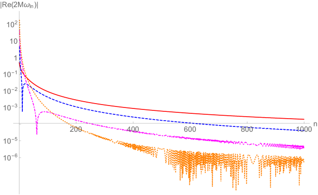
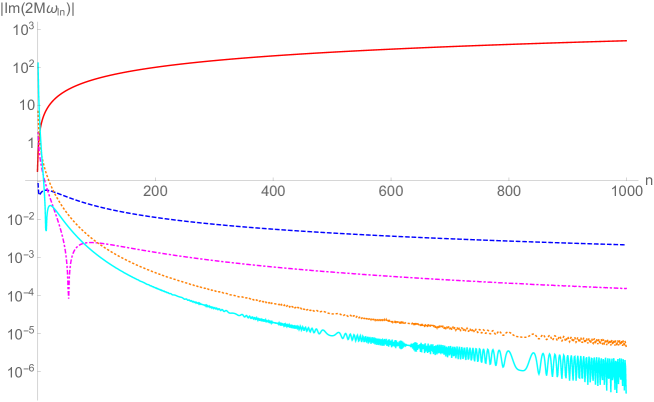
Figure 2: Comparison of the QNM frequencies $\omega_{\ell n}$ given by the asymptotic expression Eq.(44) and the numerical values provided by Berti QNM in terms of the overtone number $n$. The top plot is for $Re(\omega_{\ell n})$ and the bottom plot for $Im(\omega_{\ell n})$. The curves correspond to: Berti’s data (continuous red), Berti’s data minus the leading first (dashed blue), first two (dot-dashed magenta), first three (dotted orange) and, in the case of the imaginary part, first four (continuous cyan) orders in Eq.(44).

We finally obtain the QNM frequencies $\omega_{\ell n}$ in the following manner. We write $\sigma_{\ell n}\equiv i\omega_{\ell n}$ and expand it as $\sigma_{\ell n}=\sum_{j=-2}^{j_{m}}c_{j}/n^{j/2}$, for some upper index $j_{m}$ and some coefficients $c_{j}$ to be determined. We then replace $\sigma$ by this expansion for $\sigma_{\ell n}$ in Eq.(42) and expand the resulting QNM condition for large $n$. By imposing the condition order-by-order in $n$ we can express the coefficients $c_{j}$ in terms of the $\alpha_{k}$. The result is, with the choice $j_{m}=8$,

$$\omega_{\ell n}=-\frac{in}{2}-\frac{2i\alpha_{1}^{2}}{\pi n}-\frac{4e^{-i\pi/4}\alpha_{1}^{3}}{\pi n^{3/2}}+\frac{12\alpha_{1}^{4}}{\pi n^{2}}-\frac{8e^{i\pi/4}\alpha_{1}^{2}\left(4\alpha_{1}^{3}+\alpha_{2}\alpha_{1}-\alpha_{3}\right)}{\pi n^{5/2}}+$$ (43)

$$\frac{8i\left(37\pi\alpha_{1}^{6}+12\pi\alpha_{2}\alpha_{1}^{4}-3\alpha_{1}^{4}-12\pi\alpha_{3}\alpha_{1}^{3}-3\pi\alpha_{2}^{2}\alpha_{1}^{2}+6\pi\alpha_{4}\alpha_{1}^{2}-6\pi\alpha_{5}\alpha_{1}+3\pi\alpha_{3}^{2}\right)}{3\pi^{2}n^{3}}+$$

$$\frac{8e^{-i\pi/4}\left(38\pi\alpha_{1}^{7}+16\pi\alpha_{2}\alpha_{1}^{5}-5\alpha_{1}^{5}-16\pi\alpha_{3}\alpha_{1}^{4}-4\pi\alpha_{2}^{2}\alpha_{1}^{3}+6\pi\alpha_{4}\alpha_{1}^{3}+2\pi\alpha_{2}\alpha_{3}\alpha_{1}^{2}-6\pi\alpha_{5}\alpha_{1}^{2}+2\pi\alpha_{3}^{2}\alpha_{1}\right)}{\pi^{2}n^{7/2}}-$$

$$\frac{16\left(61\pi\alpha_{1}^{8}+28\pi\alpha_{2}\alpha_{1}^{6}-12\alpha_{1}^{6}-28\pi\alpha_{3}\alpha_{1}^{5}-6\pi\alpha_{2}^{2}\alpha_{1}^{4}+12\pi\alpha_{4}\alpha_{1}^{4}-12\pi\alpha_{5}\alpha_{1}^{3}+6\pi\alpha_{3}^{2}\alpha_{1}^{2}\right)}{\pi^{2}n^{4}}+O\left(\frac{1}{n^{9/2}}\right).$$

We only give this expression to $O(n^{-4})$ but it is straight-forward to find the QNM frequencies to arbitrary order in $n$ in terms of the $\alpha_{k}$ by systematically solving Eq.(42). We note that the QNM condition does not fully determine the coefficients of the orders $O(n)$ and $O(1)$; it only yields the condition $n\,c_{-2}+c_{0}=N/2$ on them, for $n=0,1,2,\dots$, for $N\in\mathbb{Z}$ and $c_{-2}\neq 0$. The remaining freedom corresponds to the fact that the overtone number $n$ is merely a label. We choose $c_{-2}=1/2$ and $c_{0}=0$ in agreement with the labelling scheme in Nollert (1993) which is chosen by comparison against numerical values for the QNM frequencies.

It is remarkable that the terms in the expansion show the behaviour $e^{ik\pi/4}(\mathbb{R})/n^{k/2}$ to all orders. Explicitly, using the values in Eq.(28), we have

$$\omega_{\ell n}=-\frac{in}{2}-\frac{i\lambda^{2}}{2n}+\frac{e^{-i\pi/4}\pi^{1/2}\lambda^{3}}{2n^{3/2}}+\frac{3\pi\lambda^{4}}{4n^{2}}+$$ (44)

$$\frac{e^{i\pi/4}\sqrt{\pi}\lambda^{3}\left(18\lambda^{2}(\pi+2\ln 2)-1\right)}{24n^{5/2}}+O\!\left({n^{-3}}\right).$$

We note that the term of $O\left(n^{-5/2}\right)$ corrects the corresponding term in Eq.17 Casals and Ottewill (2012b).

VI Final remarks

We have obtained a formal expansion valid to arbitrary order for large overtone number $n$ of the spin-$1$ QNM frequencies in Schwarzschild space-time. The obtention of such arbitrary-order expansion is facilitated by the fact that the regularization described in Sec.IV is only required up to second order. As observed in Casals and Ottewill (2012a), regularization seems to be required at first order in the spin-$2$ case and no regularization is required at any order in the spin-$0$ case. This indicates that a similar arbitrary-order expansion might be possible for spin-$0$ and -$2$, although their zeroth order solution is in terms of Bessel functions (see Eq.17 Casals and Ottewill (2012a)) instead of simple exponentials as in the spin-$1$ case. Astrophysically, it would be of interest to extend these results to a rotating Kerr black hole. To the best of our knowledge, the large-$n$ asymptotics for spin-$1$ QNM frequencies have not yet been determined in Kerr at any order. However, the leading-order asymptotics in Kerr have been determined for spin-$0$. In particular, it has been observed (e.g., Keshet and Hod (2007)) that the real part of these spin-$0$ frequencies in the axisymmetric case (i.e., azimuthal number $m=0$) seem to go to zero for large $n$, similarly to the spin-$1$ frequencies in Schwarzschild. It would therefore be worth investigating whether it is possible to obtain an arbitrary-order expansion for QNM frequencies in Kerr space-time for, at least, the spin-$0$ axisymmetric case, similar to the expansions we have derived in this paper for spin-$1$ in Schwarzschild.

References

• Abbott et al. (2016) B. P. Abbott, R. Abbott, T. D. Abbott, M. R. Abernathy, F. Acernese, K. Ackley, C. Adams, T. Adams, P. Addesso, R. X. Adhikari, et al. (LIGO Scientific Collaboration and Virgo Collaboration), Phys. Rev. Lett. 116, 061102 (2016), URL http://link.aps.org/doi/10.1103/PhysRevLett.116.061102.
• Schnittman (2011) J. D. Schnittman, Class. Quant. Grav. 28, 094021 (2011), eprint 1010.3250.
• Leaver (1985) E. W. Leaver, Proc. Roy. Soc. Lond. A 402, 285 (1985).
• Chandrasekhar and Detweiler (1975) S. Chandrasekhar and S. Detweiler, Proceedings of the Royal Society of London A: Mathematical, Physical and Engineering Sciences 344, 441 (1975), ISSN 0080-4630, URL http://rspa.royalsocietypublishing.org/content/344/1639/441.full.pdf.
• (5) http://www.phy.olemiss.edu/~berti/ringdown/, https://centra.tecnico.ulisboa.pt/network/grit/files/ringdown/.
• Babb et al. (2011) J. Babb, R. Daghigh, and G. Kunstatter, Phys. Rev. D84, 084031 (2011), eprint 1106.4357.
• Keshet and Neitzke (2008) U. Keshet and A. Neitzke, Phys. Rev. D78, 044006 (2008), eprint 0709.1532.
• Motl and Neitzke (2003) L. Motl and A. Neitzke, Ad. Theor. Math. Phys. 7, 307 (2003).
• Neitzke (2003) A. Neitzke (2003), eprint hep-th/0304080.
• Maassen van den Brink (2004) A. Maassen van den Brink, J. Math. Phys. 45, 327 (2004), eprint gr-qc/0303095.
• Musiri and Siopsis (2003) S. Musiri and G. Siopsis, Class. Quant. Grav. 20, L285 (2003), eprint hep-th/0308168.
• Motl (2002) L. Motl, Adv. Theor. Math. Phys. 6, 1135 (2002), eprint gr-qc/0212096.
• Musiri and Siopsis (2007) S. Musiri and G. Siopsis, Phys. Lett. B650, 279 (2007).
• Casals and Ottewill (2012a) M. Casals and A. Ottewill, Phys.Rev. D86, 024021 (2012a), eprint 1112.2695.
• Keshet and Hod (2007) U. Keshet and S. Hod, Physical Review D 76, 061501 (2007).
• Kao and Tomino (2008) H.-c. Kao and D. Tomino, Physical Review D 77, 127503 (2008).
• Casals and Ottewill (2012b) M. Casals and A. Ottewill, Phys. Rev. Lett. 109, 111101 (2012b), URL http://link.aps.org/doi/10.1103/PhysRevLett.109.111101.
• Wheeler (1955) J. A. Wheeler, Phys. Rev. 97, 511 (1955).
• Ruffini et al. (1972) R. Ruffini, J. Tiomno, and C. Vishveshwara, Lettere Al Nuovo Cimento (1971–1985) 3, 211 (1972).
• Leaver (1986) E. W. Leaver, J. Math. Phys. 27, 1238 (1986).
• Casals and Ottewill (2013) M. Casals and A. C. Ottewill, Phys.Rev. D87, 064010 (2013), eprint 1210.0519.
• Casals and Ottewill (2015) M. Casals and A. Ottewill, Phys. Rev. D 92, 124055 (2015), URL http://link.aps.org/doi/10.1103/PhysRevD.92.124055.
• Maassen van den Brink (2000) A. Maassen van den Brink, Phys. Rev. D62, 064009 (2000), eprint gr-qc/0001032.
• Bender and Orszag (1999) C. M. Bender and S. A. Orszag, Advanced Mathematical Methods for Scientists and Engineers (Springer, 1999).
• Erdelyi et al. (1953) A. Erdelyi, W. Magnus, F. Oberhettinger, and F. Tricomi, Higher Transcendental Functions (McGraw-Hill, New York, 1953).
• (26) DLMF, NIST Digital Library of Mathematical Functions, http://dlmf.nist.gov/, Release 1.0.5 of 2012-10-01, online companion to Olver et al. (2010), URL http://dlmf.nist.gov/.
• Nollert (1993) H.-P. Nollert, Physical Review D 47, 5253 (1993).
• Olver et al. (2010) F. W. J. Olver, D. W. Lozier, R. F. Boisvert, and C. W. Clark, eds., NIST Handbook of Mathematical Functions (Cambridge University Press, New York, NY, 2010), print companion to DLMF .