The impact of surface area, volume, curvature and Lennard-Jones potential to solvation modeling

Abstract

This paper explores the impact of surface area, volume, curvature and Lennard-Jones potential on solvation free energy predictions. Rigidity surfaces are utilized to generate robust analytical expressions for maximum, minimum, mean and Gaussian curvatures of solvent-solute interfaces, and define a generalized Poisson-Boltzmann (GPB) equation with a smooth dielectric profile. Extensive correlation analysis is performed to examine the linear dependence of surface area, surface enclosed volume, maximum curvature, minimum curvature, mean curvature and Gaussian curvature for solvation modeling. It is found that surface area and surfaces enclosed volumes are highly correlated to each others, and poorly correlated to various curvatures for six test sets of molecules. Different curvatures are weakly correlated to each other for six test sets of molecules, but are strongly correlated to each other within each test set of molecules. Based on correlation analysis, we construct twenty six nontrivial nonpolar solvation models. Our numerical results reveal that the Lennard-Jones (LJ) potential plays a vital role in nonpolar solvation modeling, especially for molecules involving strong van der Waals interactions. It is found that curvatures are at least as important as surface area or surface enclosed volume in nonpolar solvation modeling. In conjugation with the GPB model, various curvature based nonpolar solvation models are shown to offer some of the best solvation free energy predictions for a wide range of test sets. For example, root mean square errors from a model constituting surface area, volume, mean curvature and LJ potential are less than 0.42 kcal/mol for all test sets.

Key Words: solvation, implicit solvent model, curvature

1 Introduction

All essential biological processes, such as signaling, transcription, cellular differentiation, etc., take place in an aqueous environment. Therefore, a prerequisite of understanding such biological processes is to study the solvation process, which involves a wide range of solvent-solute interactions, including hydrogen bonding, ion-dipole, induced dipole, and dipole-dipole, hydrophobic/hydrophobic, dispersive attractions, or van der Waals forces. The most commonly available experimental measurement of the solvation process is the solvation free energy, i.e., the energy released from the solvation process. As a result, the prediction of solvation free energy has been a main theme of solvation modeling and analysis. Numerous computational models have been proposed for solvation free energy prediction, including molecular mechanics, quantum mechanics, statistical mechanics, integral equation, explicit solvent models, and implicit solvent models ^{1, 2, 3}. Each approach has its own advantages, merits and limitations. Among these models, explicit ⁴ and quantum methods ^{5, 6} are ultimately for investigating the solvation of relatively small molecules; however, a great number of degrees of freedom for large systems may lead to unmanageable computational cost. Implicit solvent models, on the contrary, can lower the number of degrees of freedom by approximating the solvent by a continuum representation and describing the solute in atomistic detail ^{7, 8, 9}.

In implicit solvent models, the total solvation free energy is divided into nonpolar and polar contributions ^{10, 11}. There is a wide range of implicit solvent models available to describe the polar solvation process; nonetheless, Poisson-Boltzmann (PB) ^{12, 7, 13, 9, 14} and generalized Born (GB) models ^{15, 16, 17, 18, 19, 20, 21} are commonly used. GB methods are very fast, but are only heuristic models for the polar solvation analysis. PB methods can be derived from fundamental theories ^{22, 23}; therefore, can offer somewhat of simple but satisfactorily accurate and robust solvation energy estimations when handling large biomolecules.

To approximate the nonpolar solute-solvent interactions in implicit solvent models, a common way is to assume the nonpolar solvation free energy being correlated with the solvent-accessible surface area (SASA) ^{24, 25}, based on the scaled-particle theory (SPT) for nonpolar solutes in aqueous solutions ^{26, 27}. However, recent studies indicate that solvation free energy may depend on both SASA and solvent-accessible volume (SAV), especially in large length scale regimes ^{28, 29}. It was pointed out that, unfortunately, SASA based solvation models do not capture the ubiquitous van der Waals (vdW) interactions near the solvent-solute interface ³⁰. Indeed, the use of SASA, SAV and solvent-solute dispersive interactions to approximate nonpolar energy significantly improves the accuracy of solvation free energy prediction ^{31, 32, 33, 34}.

One of the most important tasks in handling the implicit solvent models is to define the solute-solvent interface. Many solvation quantities such as surface area, cavitation volume, curvature of the surface and electrostatic energies significantly depend on the interface definition. The vdW surface, solvent accessible surface ³⁵, and solvent excluded surface (SES) ³⁶ have shown their effectiveness in biomolecular modeling. However, these surface definitions admit geometric singularities ^{37, 38} which result in excessive computational instability and algorithmic effort ^{39, 40, 41}. As a result, throughout the past decade, many advanced surface definitions have been developed. One of them is the Gaussian surface description ^{42, 43, 44}. Another approach is by means of differential geometry. The first curvature induced biomolecular surface was introduced in 2005 using geometric partial differential equations (PDEs) ⁴⁵. The first variational molecular surface based on minimal surface theory was proposed in 2006 ^{46, 47}. These surface definitions lead to curvature controlled smooth solvent-solute interfaces that enable one to generate a smooth dielectric profile over solvent and solute domains. This development leads to differential geometry based solvation models ^{1, 2} and multiscale models ^{48, 49, 50}. These models have been confirmed to deliver excellent solvation free energy predictions ^{33, 34}. Recently, a family of rigidity surfaces has been proposed in the flexibility-rigidity index (FRI) method, which significantly outperforms the Gaussian network model (GNM) and anisotropic network model (ANM) in protein B-factor prediction ^{51, 52, 53, 54}. Flexibility is an intrinsic property of proteins and is known to be important for protein drug binding ⁵⁵, allosteric signaling ⁵⁶ and self-assembly ⁵⁷. It must play an important role in the solvation process because of entropy effects. Therefore, FRI based rigidity surfaces, which can be regarded as generalizations of classic Gaussian surfaces ^{42, 43, 44}, may have an advantage in solvation analysis as well.

In molecular biophysics, curvature measures the variability or non-flatness of a biomolecular surface and is believed to play an important role in many biological processes, such as membrane curvature sensing, and protein-membrane and protein DNA interactions. These interactions may be described by the Canham-Helfrich curvature energy functional ⁵⁸. Due to its potential contribution to the cavitation cost, curvature of the solute-solvent surface is believed to affect the solvation free energy ⁵⁹. By using SPT, the surface tension is assumed to have a Gaussian curvature dependence ⁵⁹. The curvature in such cases is locally estimated and is a function of the solvent radius. Nevertheless, the quantitative contribution of various curvatures to solvation free energy prediction has not been investigated.

The objective of the present work is to explore the impact of surface area, volume, curvature, and Lennard-Jones potential on the solvation free energy prediction. We are particularly interested in the role of Hadwiger integrals, namely area, volume, Gaussian curvature and mean curvature, to the molecular solvation analysis. Therefore, we consider Gaussian curvature and mean curvature, as well as minimum and maximum curvatures in the present work. For the sake of accurate and analytical curvature estimation, we employ rigidity surfaces that not admit geometric singularities. Unlike the geometric flow surface in our previous work ^{1, 34}, the construction of rigidity surfaces does not require a surface evolution; accordingly, does not need parameter constraints to stabilize the optimization process. In the current models, instead of local curvature considered in other work ^{60, 61, 59}, total curvatures that are the summations of absolute local curvatures are employed to measure the total variability of solvent-solute interfaces. We show that curvature based nonpolar solvation models offer some of the best solvation predictions for a large amount of molecules.

The rest of this paper is organized as follows. Section 2 presents the theory and formulation of new solvation models. We first briefly introduce the rigidity surface for the surface definition. A generalized PB equation using a smooth dielectric function is formulated. We provide an advanced algorithm for the evaluation of surface area and surface enclosed volume. Analytical presentation for calculating various curvatures, namely Gaussian curvature, mean curvature, minimum and maximum principal curvatures are presented. Finally, we introduces a parameter learning algorithm to solvation energy prediction. Section 3 is devoted to numerical studies. First, we discuss the dataset used in this work. Over a hundred molecules of both polar and nonpolar types are employed in our numerical tests. We then discuss the models and their abbreviations to be used in this study. The numerical setups for nonpolar and polar solvation free energy calculations are described in detail. We explore the correlations between area, volume, and different types of curvatures. Based on the root mean square error (RMSE) computed between experimental and predicted results, we reveal the impact of each interested nonpolar quantities on solvation free energy prediction. The final part of Section 3 is devoted to the investigation of the most accurate and reliable solvation model. This paper ends with a conclusion.

2 Models and algorithms

2.1 Solvation models

The solvation free energy, $\Delta G$, is calculated as a sum of polar, $\Delta G^{\text{p}}$, and nonpolar, $G^{\text{np}}$, components

$$\Delta G=\Delta G^{\text{p}}+G^{\text{np}}.$$ (1)

Here, $\Delta G^{\text{p}}$ is modeled by the Poisson-Boltzmann theory. For the nonpolar contribution, we consider the following nonpolar solvation free functional

$$\Delta G^{\text{np}}=\gamma A+pV+\sum_{j}\lambda_{j}C_{j}+\rho_{0}\int_{\Omega_{s}}U^{\text{vdW}}\mathrm{d}\mathbf{r},$$ (2)

where $A$ and $V$ are, respectively, the surface area and surface enclosed volume of the solute molecule of interest. Additionally, $\gamma$ is the surface tension and $p$ is the hydrodynamic pressure difference. We denote $C_{j}$ and $\lambda_{j}$ respectively curvatures and associated bending coefficients of the molecular surface. Thus, the index $j$ runs from maximum curvature, minimum curvature, mean curvature to Gaussian curvature. Here $\rho_{0}$ is the solvent bulk density, and $U^{\text{vdW}}$ is the van der Waals (vdW) interaction approximated by the Lennard-Jones potential. The final integral is computed solely over solvent domain $\Omega_{s}$. One can turn off certain terms in Eq. (2) to arrive at simplified models.

2.2 Rigidity surface

Flexibility-rigidity index (FRI) has been shown to significantly outperform other methods, such the Gaussian network model (GNM) and anisotropic network model (ANM), in protein flexibility analysis or B-factor prediction over hundreds of molecules ^{51, 52, 53, 54}. Given a molecule with $N$ atoms, we denote $\mathbf{r}_{j}$ the position of $j$th atom, $\|\mathbf{r}-\mathbf{r}_{j}\|$ the Euclidean distance between a point $\mathbf{r}$ and atom $\mathbf{r}_{j}$. In our FRI method, commonly used correlation kernels or statistical density estimators ^{51, 52, 62} include generalized exponential functions

$$\mathbf{\Phi}\left(\|\mathbf{r}-\mathbf{r}_{j}\|;\eta_{j}\right)=e^{{-\left(\|\mathbf{r}-\mathbf{r}_{j}\|/\eta_{j}\right)}^{\kappa}},\quad\kappa>0,$$ (3)

and generalized Lorentz functions

$$\mathbf{\Phi}\left(\|\mathbf{r}-\mathbf{r}_{j}\|;\eta_{j}\right)=\frac{1}{1+\left(\frac{\|\mathbf{r}-\mathbf{r}_{j}\|}{\eta_{j}}\right)^{\nu}},\quad\nu>0,$$ (4)

where $\eta_{j}$ is a scale parameter. An atomic rigidity function $\mu(\mathbf{r})$ for an arbitrary point $\mathbf{r}$ on the computational domain can be defined as

$$\mu(\mathbf{r})=\sum_{j=1}^{N}w_{j}(\mathbf{r})\mathbf{\Phi}\left(\|\mathbf{r}-\mathbf{r}_{j}\|;\eta_{j}\right),$$ (5)

where $w_{j}(\mathbf{r})$ is a weight function. The atomic rigidity function $\mu(\mathbf{r})$ measures the atomic density at position $\mathbf{r}$. This intepretation can be easily verified since if we choose $w_{j}(\mathbf{r})$ such that

$$\int\mu(\mathbf{r})d{\bf r}=1.$$

Then the atomic rigidity function $\mu(\mathbf{r})$ becomes a probability density distribution such that $\mu(\mathbf{r})d{\bf r}$ is the probability of finding all the $N$ atoms in an infinitesimal volume element $d{\bf r}$ at a given point ${\bf r}\in\mathbb{R}^{3}$. For $\mathbf{\Phi}\left(\|\mathbf{r}-\mathbf{r}_{j}\|;\eta_{j}\right)=e^{{-\left(\|\mathbf{r}-\mathbf{r}_{j}\|/\eta_{j}\right)}^{2}}$, one can analytically choose $w_{j}(\mathbf{r})=\frac{1}{N}\left(\frac{1}{\pi\eta_{j}^{2}}\right)^{\frac{3}{2}}$ to normalize atomic rigidity function $\mu(\mathbf{r})$.

For simplicity, in this work we just employ the Gaussian kernel, i.e., generalized exponential kernel with $\kappa=2$, $\eta_{j}=r^{\text{vdW}}_{j}$ (i.e., the vdW radius of atom $j$), and $w_{j}=1$ for all $j=1,2,\cdots,N$. Other FRI kernels are found to deliver very similar results. Our rigidity surfaces can be regarded as a generalization of Gaussian surfaces ^{63, 18}.

2.3 Smooth rigidity function-based dielectric function

We denote $\Omega$ the total domain, and $\Omega$ is divided into two regions, i.e., aqueous solvent domain $\Omega_{s}$ and solute molecular domain $\Omega_{m}$. Our ultimate goal is to construct a smooth dielectric function in a similar way to that of differential geometry based solvation models as follows ^{48, 1, 2}

$$\epsilon(\mu)=(1-\mu)\epsilon_{s}+\mu\epsilon_{m},$$ (6)

where $\epsilon_{s}$ and $\epsilon_{m}$ are the dielectric constants of the solvent and solute, respectively. However the total atomic density described in (5) exceeds 1 in many cases. As a result, we normalize the atomic rigidity function as

$$\bar{\mu}(\mathbf{r})=\frac{1}{\max\limits_{\mathbf{r}\in\Omega}\mu(\mathbf{r})}\mu(\mathbf{r}).$$ (7)

Nonetheless, the dielectric function (6) is still not applicable since the characteristic function $1-\bar{\mu}$ may not capture the commonly defined solvent domain. This is due to the fact that the value of $\bar{\mu}(\mathbf{r})$ could be less than 1 inside the biomolecule. As a result, we define the molecular domain as $\{\mathbf{r}\in\Omega|\mu(\mathbf{r})\geq\beta\}$, where $\beta$ is a cut-off value defined in the protocol to attain the best fitting against other PB solvers, such as MIBPB ⁶⁴. By doing so, the dielectric function (6) will be modified as the following

$$\epsilon(\bar{\mu}(\mathbf{r}))=\left\{\begin{array}[]{ll}\epsilon_{m},&\text{if $\bar{\mu}(\mathbf{r})\geq\beta$,}\\ \displaystyle\left(1-\frac{\bar{\mu}}{\beta}\right)\epsilon_{s}+\frac{\bar{\mu}}{\beta}\epsilon_{m},&\text{if $\bar{\mu}(\mathbf{r})<\beta$.}\end{array}\right.$$ (10)

2.4 Generalized Poisson-Boltzmann (GPB) equation

With smooth dielectric profile being defined in (10), we arrive at the GPB equation in an ion-free solvent

$$-\nabla\cdot\left(\epsilon(\bar{\mu})\nabla\phi({\bf r})\right)=\bar{\mu}\rho_{m}({\bf r}),$$ (11)

where $\phi$ is the electrostatic potential, $\rho_{m}({\bf r})=\sum_{i}^{N_{m}}Q_{i}\delta({\bf r-r}_{i})$ represents the fixed charge density of the solute. Here $Q(\mathbf{r}_{i})$ is the partial charge at $\mathbf{r_{i}}$ in the solute molecule, and $N_{m}$ is the total number of partial charges.

Let $\Omega$ be the computational domain of the GPB equation. Without considering the salt molecule in the solvent, we employ the Dirichlet boundary condition via a Debye-Hückel expression for the GPB equation

$$\phi(\mathbf{r})=\sum_{i=1}^{N_{m}}\frac{Q_{i}}{\epsilon_{s}\|\mathbf{r}-\mathbf{r}_{i}\|},\quad\forall\mathbf{r}\in\partial\Omega.$$ (12)

The electrostatic solvation free energy, $\Delta G^{\text{p}}$, is calculated by

$$\Delta G^{\text{p}}=\frac{1}{2}\sum_{i=1}^{N_{m}}Q(\mathbf{r}_{i})\left(\phi(\mathbf{r}_{i})-\phi_{0}(\mathbf{r}_{i})\right),$$ (13)

where $\phi$ and $\phi_{0}$ are, respectively, the electrostatic potential in the presence of the solvent and vacuum. In other words, $\phi$ is a solution of the GPB equation (11), and homogeneous solution $\phi_{0}$ of the GPB equation is obtained by setting dielectric function $\epsilon(\bar{\mu})=\epsilon_{m}$ in the whole computational domain $\Omega$.

2.5 Surface area and surface-enclosed volume

The surface integral for a density function $f$ over $\Gamma$ in the domain $\Omega$ with a uniform mesh can be evaluated by ^{65, 66, 67}

$$\int_{\Gamma}f(x,y,z)dS\approx\sum_{(i,j,k)\in I}\left(f(x_{0},y_{j},z_{k})\frac{|n_{x}|}{h}+f(x_{i},y_{0},z_{k})\frac{|n_{y}|}{h}+f(x_{i},y_{j},z_{0})\frac{|n_{z}|}{h}\right)h^{3},$$ (14)

where $(x_{0},y_{j},z_{k})$ is the intersecting point between the interface $\Gamma$ and the $x$ mesh line going through $(i,j,k)$, and $n_{x}$ is the $x$ component of the unit normal vector at $(x_{0},y_{j},z_{k})$. Similar definitions are used for the $y$ and $z$ directions. We only carry out the calculation (14) in a small set of irregular grid points, denoted as $I$. Here, the irregular grid points are defined to be the points associated with neighbor point(s) from the other side of the interface $\Gamma$ in the second order finite difference scheme ³⁹. In this case, $I$ will contain the irregular points near interface $\Gamma$. Finally, $h$ is the uniform grid spacing. The volume integral can be simply approximated by

$$\int_{\Omega_{m}}fd\mathbf{r}\approx\sum_{(i,j,k)\in J}f(x_{i},y_{j},z_{k})h^{3},$$ (15)

where $\Omega_{m}$ is the domain enclosed by $\Gamma$, and $J$ is the set of all grid points inside $\Omega_{m}$. By considering the density function $f=1$, Eqs. (14) and (15) can be respectively used for the surface area and volume calculations.

2.6 Curvature calculation

The evaluation of the curvatures for isosurface embedded volumetric data, $S(x,y,z)$, has been reported in the literature ^{47, 68, 69}. In general, there are two approaches for the curvature evaluation. The first method is to invoke the first and second fundamental forms in differential geometry, the another one is to make use of the Hessian matrix method ⁷⁰. Since both of these algorithms yield the same results as shown in our earlier work ⁶⁹, only the first approach is employed in the present work. To this end, we immediately provide the formulation for Gaussian curvature ($K$) and mean curvature ($H$) by means of the first and second fundamental forms ^{68, 69}

$$K= \frac{2S_{x}S_{y}S_{xz}S_{yz}+2S_{x}S_{z}S_{xy}S_{yz}+2S_{y}S_{z}S_{xy}S_{xz}}{g^{2}}$$

$$-\frac{2S_{x}S_{z}S_{xz}S_{yy}+2S_{y}S_{z}S_{xx}S_{yz}+2S_{x}S_{y}S_{xy}S_{zz}}{g^{2}}$$

$$+\frac{S_{z}^{2}S_{xx}S_{yy}+S_{x}^{2}S_{yy}S_{zz}+S_{y}^{2}S_{xx}S_{zz}}{g^{2}}$$

$$-\frac{S_{x}^{2}S_{yz}^{2}+S_{y}^{2}S_{xz}^{2}+S_{z}^{2}S_{xy}^{2}}{g^{2}},$$ (16)

and

$$H=\frac{2S_{x}S_{y}S_{xy}+2S_{x}S_{z}S_{xz}+2S_{y}S_{z}S_{yz}-(S_{y}^{2}+S_{z}^{2})S_{xx}-(S_{x}^{2}+S_{z}^{2})S_{yy}-(S_{x}^{2}+S_{y}^{2})S_{zz}}{2g^{\frac{3}{2}}},$$ (17)

where $g=S_{x}^{2}+S_{y}^{2}+S_{z}^{2}$. With determined Gaussian and mean curvatures, the minimum, $\kappa_{1}$, and maximum, $\kappa_{2}$, can be evaluated by

$$\kappa_{1}=\min\{H-\sqrt{H^{2}-K},H+\sqrt{H^{2}-K}\},\quad\kappa_{2}=\max\{H-\sqrt{H^{2}-K},H+\sqrt{H^{2}-K}\}.$$ (18)

We apply the formulations (16), (17) and (18) for curvature calculations of rigidity surfaces. Again, we only consider generalized exponential kernel with $\kappa=2$ and $w_{j}=1$ for all $j=1,2,\cdot,N$ in this paper. As a result, the atomic rigidity function $\mu(\mathbf{r})$, defined in (3) and (5), become

$$\mu(\mathbf{r})=\sum_{j=1}^{N}e^{-\left(\frac{\|r-r_{j}\|}{\eta_{j}}\right)^{2}}=\sum_{j=1}^{N}e^{-\frac{(x-x_{j})^{2}+(y-y_{j})^{2}+(z-z_{j})^{2}}{\eta_{j}^{2}}}.$$ (19)

Note that derivatives of $\mu$ can be analytically attained. Therefore, by replacing $S$ with $\mu$ in various curvature formulas, we obtain analytical expressions for different curvatures of FRI based rigidity surfaces. As a result, the calculation of various curvatures is very simple and robust for rigidity surfaces.

2.7 Optimization algorithm

In this section, we present an algorithm, inspired by the algorithm 2 in our earlier work ³⁴, to optimize the parameters appearing in the nonpolar component. In this work, we utilize the 12-6 Lennard-Jones potential to model the van der Waals interaction $U_{i}^{\text{vdW}}$ regarding an atom of type $i$

$$U_{i}^{\text{vdW}}(\mathbf{r})=\epsilon_{i}\left[\left(\frac{\sigma_{i}+\sigma_{s}}{\|\mathbf{r}-\mathbf{r}_{i}\|}\right)^{12}-2\left(\frac{\sigma_{i}+\sigma_{s}}{\|\mathbf{r}-\mathbf{r}_{i}\|}\right)^{6}\right],$$ (20)

where $\epsilon_{i}$ is the well-depth parameter, $\sigma_{i}$ and $\sigma_{s}$ are, respectively, the radii of the atom of type $i$ and solvent. Here $\mathbf{r}$ is the location of an arbitrary point in the solvent domain, and $\mathbf{r}_{i}$ is the location of the atom of type $i$. Since the integral of the Lennard-Jones potential term involves in the solvent bulk density $\rho_{0}$, the fitting parameter for the van der Waals interaction of the atom of type $i$ will be $\tilde{\epsilon}_{i}\doteq\rho_{0}\epsilon_{i}$. Assume that we have a training group containing $n$ molecules, the process of calculating solvation free energy will give us the following quantities for the $j$th $(j=1,2,\cdots,n)$ molecule

$$\left\{\Delta G^{\text{p}}_{j},A_{j},V_{j},C_{1j},C_{2j},C_{3j},C_{4j},\left(\sum_{i=1}^{N_{m}}\delta^{1}_{i}\int_{\Omega_{s}}U_{1}^{\text{vdW}}(\mathbf{r})\mathrm{d}\mathbf{r}\right)_{j},\cdots,\left(\sum_{i=1}^{N_{m}}\delta^{N_{t}}_{i}\int_{\Omega_{s}}U_{N_{t}}^{\text{vdW}}(\mathbf{r})\mathrm{d}\mathbf{r}\right)_{j}\right\},$$ (21)

where $N_{m}$ and $N_{t}$ are the number of atoms and the number of atom types in each individual molecule, respectively and $C_{ij}$ denotes the $i$th curvature for the $j$th molecule. Here $\delta^{k}_{i}$ is defined as follows

$$\delta^{k}_{i}=\left\{\begin{array}[]{ll}1,&\text{if atom $i$ belongs to type $k$,}\\ 0,&\text{otherwise,}\end{array}\right.$$ (24)

where $k=1,2,\cdots,N_{t}$ and $i=1,2,\cdots,N_{m}$. We denote the parameter set for the current training group as $\mathbf{P}=\left\{\gamma,p,\lambda_{1},\cdots,\lambda_{4},\tilde{\epsilon}_{1},\tilde{\epsilon}_{2},\cdots,\tilde{\epsilon}_{N_{t}}\right\}$. The solvation free energy for molecule $j$ will be then predicted by

$$\Delta G_{j}= \Delta G^{\text{p}}_{j}+\gamma A_{j}+pV_{j}+\sum_{i}\lambda_{i}C_{ij}+\tilde{\epsilon}_{1}\left(\sum_{i=1}^{N_{m}}\sigma^{1}_{i}\int_{\Omega_{s}}U_{1}^{\text{vdW}}(\mathbf{r})\mathrm{d}\mathbf{r}\right)_{j}$$

$$+\cdots+\tilde{\epsilon}_{N_{t}}\left(\sum_{i=1}^{N_{m}}\sigma^{N_{t}}_{i}\int_{\Omega_{s}}U_{N_{t}}^{\text{vdW}}(\mathbf{r})\mathrm{d}\mathbf{r}\right)_{j}.$$ (25)

It is noted that the fitting parameter of corresponding vanishing term will set to $0$ in the solvation free energy calculation (25). We denote a vector of predicted solvation energies for the given molecular group as $\Delta\mathbf{G}(\mathbf{P})=(\Delta G_{1},\Delta G_{2},\cdots,\Delta G_{n})$ which depends on the parameter set $\mathbf{P}$. In addition, we denote a vector of the corresponding experimental solvation free energy as $\Delta\mathbf{G}^{\text{Exp}}=(\Delta G^{\text{Exp}}_{1},\Delta G^{\text{Exp}}_{2},\cdots,\Delta G^{\text{Exp}}_{n})$. We then optimize the parameter set $\mathbf{P}$ by solving the following minimization problem

$$\min_{\mathbf{P}}\left(\|\Delta\mathbf{G}(\mathbf{P})-\Delta\mathbf{G}^{\text{Exp}}\|_{2}\right),$$ (26)

where $\|*\|_{2}$ denotes the $L_{2}$ norm of the quantity $*$. Optimization problem (26) is a standard one which can be solved by many available tools. In this work, we employ CVX software ⁷¹ to deal with it.

Unlike our previous work ³⁴, we only need to generate the fixed molecular surface and solve the GPB equation (11) one time. We will then utilize the optimization process (26) with obtained quantities to achieve the optimized parameter set $\mathbf{P}$.

3 Results and discussions

3.1 Data sets

To study the impact of area, volume, curvature and Lennard-Jones potential on the solvation free energy prediction, we employ a large number of solute molecules with accurate experimental solvation values. These molecules are of both polar and nonpolar types and are divided into six groups: the SAMPL0 test set ⁷² with 17 molecules, alkane set with 35 molecules, alkene set with 19 molecules, ether set with 15 molecules, alcohol set with 23 molecules, and phenol set with 18 molecules sets ⁷³. The charges of the SAMPL0 set are taken from the OpenEye-AM1-BCC v1 parameters ⁷⁴, while their atomic coordinates and radii are based on the ZAP-9 parametrization ⁷². The structural conformations for the other groups are adopted from FreeSolv⁷³ with their parameter and coordinate information being downloaded from Mobley’s homepage http://mobleylab.org/resources.html.

3.2 Model abbreviation

Table 1: Model terminologies

Symbols	Meaning
$\mathbf{A}$	$G^{\text{np}}$ contains a area term
$\mathbf{V}$	$G^{\text{np}}$ contains a volume term
$\mathbf{L}$	$G^{\text{np}}$ contains a Lennard-Jones potential term
$\mathbf{k_{1}}$	$G^{\text{np}}$ contains a minimum curvature term
$\mathbf{k_{2}}$	$G^{\text{np}}$ contains a maximum curvature term
$\mathbf{H}$	$G^{\text{np}}$ contains a mean curvature term
$\mathbf{K}$	$G^{\text{np}}$ contains a Gaussian curvature term

It is noted that if we only consider area, volume and van der Waals interaction in nonpolar component computations, we would arrive at the formulation already discussed in the literature ^{32, 1}. However, the nonpolar component in this work includes additional curvature terms. To investigate the impact of area, volume, Lennard-Jones potential and curvature on the solvation free energy prediction, we benchmark different models consisting of various terms in nonpolar free energy functionals. To this end, we use the symbols listed in Table 1 to label a model if it includes the corresponding terms in the nonpolar solvation free functional. For example, model $\mathbf{A}$ only considers the surface area term, whereas model $\mathbf{AVL}$ incorporates area (A), volume (V) and Lennard-Jones potential (L) terms in nonpolar energy calculations.

3.3 Polar and nonpolar calculations

In this work, we employ rigidity surface ^{51, 52}, discussed in Section 2.2, as the surface representation of a solvent-solute interface. For simplicity, we implement the Gaussian kernel for all tests, while other FRI kernels deliver similar results.

Polar part

By following the paradigm for constructing a smooth dielectric function in differential geometry based solvation models ^{48, 1}, we propose a smooth rigidity-based dielectric function as in Eq. (10). The generalized Poisson-Boltzmann (GPB) equation described in Eq. (11) is used. For the current framework, we consider the solvent environment without salt and there is only one solvent component, water. The polar solvation energy is then calculated as the difference of the GPB energies in water and in a vacuum, and the detail of this representation is offered in Section 2.4. Similar results are obtained if we create a sharp interface and then employ a standard PB solver to compute the polar solvation energy.

In all calculations, the rigidity surface is constructed based on the cut-off value being $\beta=0.09$, and the dielectric constants for solute and solvent regions are set to 1 and 80, respectively. In addition, the grid spacing is set to $0.2$ Å. The computational domain is the bounding box of the molecular surface with an extra buffer length of $3$ Å. The changes in RMS errors are less than 0.02 kcal/mol when the buffer length is extended to 6 Å. Since the dielectric profile in the GPB equation is smooth throughout the computational domain, one can easily make use of the standard second order finite difference scheme to numerically solve the GPB equation. Then, a standard Krylov subspace method based solver ^{1, 2} is employed to handle the resulting algebraic equation system.

Nonpolar part

To estimate the surface area and surface enclosed volume for a rigidity surface, we utilize a stand-alone algorithm based on the marching cubes method, and the detail of this procedure is referred to Section 2.5. Thanks to the use of the rigidity surface, the curvature of a solvent-solute interface can be analytically determined instead of using numerical approximations as in our earlier differential geometry model ⁶⁹. To prevent the curvature from canceling each other at different grid points, we construct total curvatures defined as

$$C_{j}=\sum_{\mathbf{r}_{i}\in I}|c_{j}(\mathbf{r}_{i})|h^{2},$$ (27)

where $\mathbf{r}_{i}$ is the position of the $i$th grid point, $I$ is a set of irregular grid points in the region of the solvent-solute boundary ^{39, 40, 41} and $h$ is the mesh size of the uniform computational domain. Here $c_{j}(\mathbf{r}_{i})$ is the $j$th type of curvature at position $\mathbf{r}_{i}$, and index $j$ runs through minimum, maximum, mean and Gaussian curvatures. Since the full standard 12-6 Lennard-Jones potential improves accuracy of the solvation free energy prediction ^{3, 34}, it is utilized to model the vdW interaction $U^{\text{vdW}}$ in the current work.

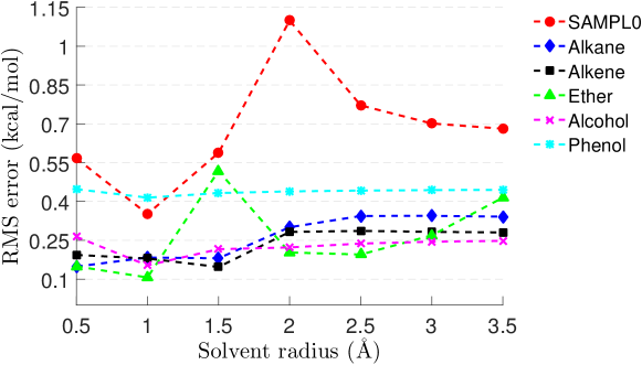
Figure 1: The relations between the solvent radii and the RMS errors for model $\mathbf{AVHL}$. Red circle: SAMPL0 set; blue diamond: alkane set; black square: alkene set; green triangle: ether set ; pink cross: alcohol set; cyan asterisk: phenol set.

Similar to our previous work ³⁴, an optimization process as discussed in Section 2.7 is applied to determine the optimal parameters for the nonpolar free energy calculations. Unfortunately, the involvement of the solvent radius in the Lennard-Jones potential term features a high nonlinearity. Consequently, it cannot be incorporated into the parameter optimization. Instead, we resort to a brute force approach to determine the most favorable solvent radius for six molecular sets including SAMPL0, alkane, alkene, ether, alcohol, and phenol groups. The value of $\sigma_{s}$ that mostly produces the smallest RMS error between predicted and experimental solvation free energies will be employed in all numerical calculations. By considering model $\mathbf{AVHL}$, we depict the relations between RMS errors and the solvent radii varying from $0.5$ Å to $3.5$ Å with the increment of $0.5$ Å in Fig. 1. This figure reveals that the use of $\sigma_{s}=1$ Å will give us the smallest RMS errors in all test sets except alkane and alkene sets. Therefore, we utilize solvent radius $1$ Å for the current work.

3.4 Correlations between area, volume and curvatures

Understanding the correlation or non-correlation between different modeling components is important for analyzing solvation models. A strong correlation between any pair of components indicates their strong linear dependence and redundancy in optimization based solvation modeling. While a weak correlation implies their complementary roles in an optimization based solvation modeling.

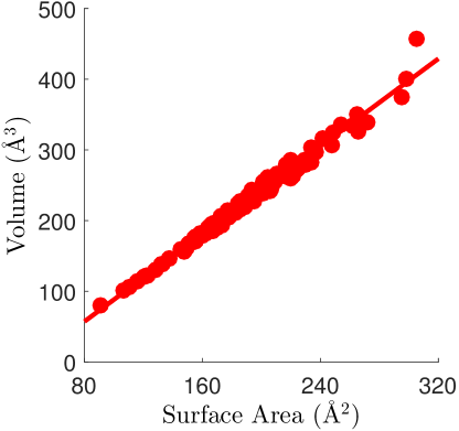
Figure 2: Area versus volume over 127 molecules in all six groups. $R^{2}=0.99$, and fitting line: $y=1.55x-66.51$.

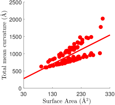
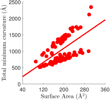
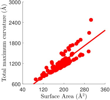
Figure 3: Area versus curvatures over 127 molecules in all six groups. $R^{2}$ values of the best fitting lines are 0.47, 0.22, 0.32 and 0.73, respectively for mean, Gaussian, minimum and maximum curvatures.

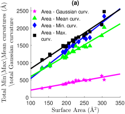
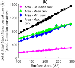
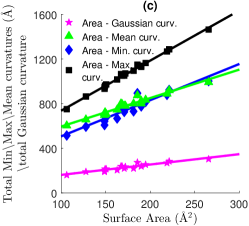
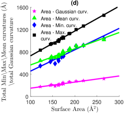
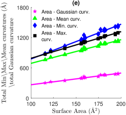
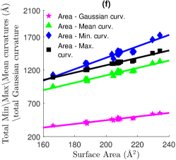
Figure 4: Area versus minimum, maximum, mean, and Gaussian curvatures. Blue diamond : area versus minimum curvature, black square: area versus maximum curvature, green triangle: area versus mean curvature, pink star: area versus Gaussian curvature. Six groups are labeled as: (a) SAMPL0 set, (b) alkane set, (c) alkene set, (d) ether set, (e) alcohol set, and (f) phenol set.

Correlation between areas and volumes

Figure 2 shows the correlation between surface areas and surface enclosed volumes for 127 molecules studied in this work. Apparently, their surface areas and surface enclosed volumes are highly correlated to each other. The best fitting line and $R^{2}$ found in this numerical experiment are, respectively, $y=1.55x-66.51$ and $0.99$. A similar correlation was reported in the literature ⁷⁵. Therefore, it is computationally inefficient to simultaneously include both area and volume components in a solvation model. However, physically, it is perfectly fine to have both area and volume in a solvation model as surface area represents the energy induced by the surface tension, whereas surface enclosed volume describes the work required to create a cavity in the solvent for a solute molecule. Mathematically, the correlation between surface areas and volumes of a group of solute molecules can be due to their similarity in their sphericity measurements ⁷⁶. Therefore, the surface areas and volumes of lipid bilayer sheets will not be correlated with those of micelles or liposomes.

Table 2: $R^{2}$ values and best fitting lines between area and curvature measurements.

Group	area vs min. curv.			area vs max. curv.			area vs mean curv.			area vs Gaussian curv.
	fitting line	$R^{2}$		fitting line	$R^{2}$		fitting line	$R^{2}$		fitting line	$R^{2}$
SAMPL0	$y=8.07x-262.51$	0.96		$y=6.86x+141.72$	0.95		$y=6.08x-5.05$	0.95		$y=1.86x+22.05$	0.90
Alkane	$y=2.75x+210.87$	0.95		$y=4.21x+299.83$	0.99		$y=2.34x+340.21$	0.98		$y=0.76x+80.84$	0.93
Alkene	$y=3.24x+183.15$	0.90		$y=4.49x+288.34$	0.99		$y=2.55x+340.27$	0.95		$y=0.93x+68.51$	0.87
Ether	$y=3.83x+70.92$	0.91		$y=4.45x+283.94$	0.99		$y=2.91x+273.88$	0.94		$y=1.09x+38.78$	0.91
Alcohol	$y=6.89x+87.63$	0.99		$y=5.29x+261.34$	1.00		$y=4.69x+221.01$	0.99		$y=2.32x+34.15$	0.99
Phenol	$y=8.58x-330.11$	0.94		$y=5.56x+161.15$	0.98		$y=5.56x+9.16$	0.95		$y=2.77x-108.17$	0.93

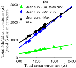
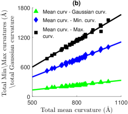
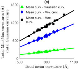
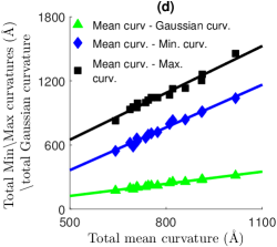
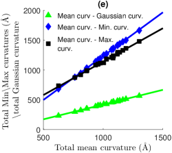
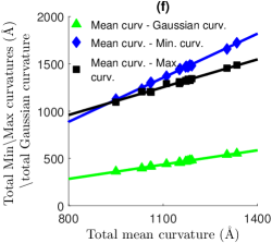
Figure 5: Mean curvature versus minimum, maximum, and Gaussian curvatures. Green triangle: mean curvature versus Gaussian curvature, blue diamond: mean curvature versus minimum curvature, black square: mean curvature versus maximum curvature. Six groups are labeled as: (a) SAMPL0set, (b) alkane set, (c) alkene set, (d) ether set, (e) alcohol set, and (f) phenol set.

Table 3: $R^{2}$ values and best fitting lines between mean curvature and another types of curvatures.

Group	mean curv. vs min. curv.			mean curv. vs max. curv.			mean curv. vs Gaussian curv.
	fitting line	$R^{2}$		fitting line	$R^{2}$		fitting line	$R^{2}$
SAMPL0	$y=1.42x-34.72$	0.99		$y=1.16x+19.71$	0.98		$y=0.54x-12.48$	0.97
Alkane	$y=1.19x-32.63$	0.99		$y=1.79x-49.63$	0.99		$y=0.34x-4.92$	0.96
Alkene	$y=1.27x-40.51$	0.98		$y=1.70x-42.13$	0.98		$y=0.38x-8.32$	0.96
Ether	$y=1.33x-49.84$	0.99		$y=1.52x-19.49$	0.97		$y=0.40x-12.01$	0.98
Alcohol	$y=1.52x-19.20$	1.00		$y=1.08x+5.87$	1.00		$y=0.89x-13.79$	1.00
Phenol	$y=1.57x-26.77$	1.00		$y=1.03x+17.22$	0.98		$y=0.87x-18.57$	0.99

Correlation between areas and curvatures

We next investigate the correlations between surface areas and four different types of curvatures for 127 molecules. Our results are depicted in Fig. 3. Obviously, the correlation between surface areas and maximum curvatures is the highest among curvature counterparts. The $R^{2}$ value for the best fitting line is 0.73. However, mean curvatures, Gaussian curvatures and minimum curvatures do not relate to surface areas very well. Their $R^{2}$ values for the best fitting lines are 0.47, 0.22 and 0.32, respectively, which are unsatisfactory.

These results are expected because maximum curvatures are mostly rendered from the convex surfaces of the molecular rigidity surface manifold, whereas minimum curvatures correspond to the concave surfaces of the molecular rigidity surface manifold. Topologically, in spirit of Morse-Smale theory, a family of extreme values of minimum curvatures defined at various isosurfaces gives rise to a natural decomposition of molecular rigidity density and leads to “rigidity complex”. The mean curvature is the average of minimum and maximum curvatures. The Gaussian curvature, as the product of two principle curvatures, correlates the least to the surface area for 127 molecules studied. Therefore, compared to volumes, Gaussian and minimum curvatures are complementary to surface areas and thus, are more useful for solvation modeling in general.

However, a careful examination of Fig. 3 reveals certain linear features. To understand the origin of the data alignment in Fig. 3, we analyze the correlations between surface areas and curvatures in six test sets. Figure 4 depicts these correlations. Obviously, there are good correlations in each test set. The best fitting lines and $R^{2}$ values of the corresponding date are reported in Table 2. These data further indicate that surface area and curvature quantities in each test set are well correlated; specifically, $R^{2}$ values of them are always larger than $0.89$. By averaging over six groups, the maximum curvature has the highest correlation with surface area, following by mean curvature, minimum curvature and Gaussian curvature. Surprisingly, for mean, Gaussian and minimum curvatures, such well correlations only occur in individual test sets.

Moreover, the slopes of fitting lines in Table 2 indicates that the curvatures and areas in alkane, alkene and ether sets are well correlated. A possible reason for this correlation is that structures of the molecules in these three groups are quite similar to each other.

Correlation between different curvatures

Additionally, we are interested in finding the correlations between different curvatures. Such a finding enables us to determine how many curvature terms in an efficient solvation model. Figure 5 depicts the correlation data between mean curvature and other types of curvatures for each group. As expected, different types of curvature are correlated to each other extremely well for each group. Table 3 provides the best fitting lines and $R^{2}$ values for such correlations, and we can see that $R^{2}$ for any case is always higher than $0.95$. Based on this correlation analysis, it is clear that different curvatures will have the same modeling effect in solvation analysis and thus at most one type of curvature term is needed in an efficient solvation model. The correlations among different curvatures for all 127 molecules are illustrated in Fig. S1 in Supporting Information.

3.5 The influence of surface area, volume, curvatures and Lennard-Jones potential on the accuracy of solvation free energy prediction

Table 4: The solvation free energy prediction for the SAMPL0 set with different models. Energy is in the unit of kcal/mol.

		M01	M02	M03	M04	M05	M06	M07	M08	M09	M10	M11	M12	M13	M14	M15	M16	M17
	$\Delta G^{\text{Exp}}$72	-8.84	-2.38	-1.93	1.07	-11.01	-9.76	-4.23	-4.97	-3.28	-5.05	-6.00	-2.93	-6.34	-3.54	-1.43	-4.08	-9.81
	$\Delta G^{\text{p}}$	-5.27	-2.10	-2.17	-1.45	-4.43	-3.82	-1.52	-3.78	-0.99	-1.98	-3.54	-1.37	-3.45	-0.97	-1.14	-3.43	-4.93
$\mathbf{H}$	$\Delta G^{\mathbf{H}}$	-2.79	-1.83	-1.78	-3.17	-2.33	-2.29	-2.01	-2.32	-2.09	-1.43	-2.31	-1.51	-2.07	-2.20	-1.85	-1.85	-1.31
	$\Delta G$	-8.06	-3.93	-3.95	-4.62	-6.76	-6.10	-3.54	-6.10	-3.08	-3.41	-5.85	-2.89	-5.52	-3.18	-2.99	-5.27	-6.24
	Error	-0.78	1.55	2.02	5.69	-4.25	-3.66	-0.69	1.13	-0.20	-1.64	-0.15	-0.04	-0.82	-0.36	1.56	1.19	-3.57
	RMSE	2.34
$\mathbf{A}$	$\Delta G^{\mathbf{A}}$	-2.94	-1.94	-1.92	-3.01	-2.61	-2.50	-2.03	-2.22	-2.14	-1.52	-2.45	-1.51	-2.17	-2.31	-1.88	-1.96	-1.30
	$\Delta G$	-8.21	-4.04	-4.09	-4.45	-7.04	-6.32	-3.55	-6.00	-3.13	-3.50	-5.99	-2.88	-5.62	-3.28	-3.02	-5.39	-6.23
	Error	-0.63	1.66	2.16	5.52	-3.97	-3.44	-0.68	1.03	-0.15	-1.55	-0.01	-0.05	-0.72	-0.26	1.59	1.31	-3.58
	RMSE	2.27
$\mathbf{L}$	$\Delta G^{\mathbf{L}}$	-3.37	-0.28	-1.79	2.52	-4.29	-4.21	-2.36	-2.49	-2.99	-1.96	-2.89	-1.98	-2.57	-3.13	-0.29	-1.76	-6.03
	$\Delta G$	-8.64	-2.38	-3.96	1.07	-8.72	-8.02	-3.88	-6.27	-3.98	-3.94	-6.43	-3.36	-6.02	-4.10	-1.43	-5.19	-10.96
	Error	-0.20	0.00	2.03	0.00	-2.29	-1.74	-0.35	1.30	0.70	-1.11	0.43	0.43	-0.32	0.56	0.00	1.11	1.15
	RMSE	1.07
$\mathbf{A}$ $\mathbf{H}$	$\Delta G^{\mathbf{A}}$	-40.93	-27.04	-26.78	-41.87	-36.39	-34.89	-28.24	-30.98	-29.79	-21.16	-34.10	-21.03	-30.23	-32.14	-26.13	-27.36	-18.10
	$\Delta G^{\mathbf{H}}$	37.41	24.46	23.83	42.47	31.18	30.61	26.95	31.13	28.01	19.12	30.96	20.27	27.66	29.52	24.79	24.74	17.55
	$\Delta G$	-8.79	-4.68	-5.11	-0.85	-9.64	-8.10	-2.82	-3.64	-2.77	-4.02	-6.68	-2.13	-6.02	-3.58	-2.47	-6.04	-5.48
	Error	-0.05	2.30	3.18	1.92	-1.37	-1.66	-1.41	-1.33	-0.51	-1.03	0.68	-0.80	-0.32	0.04	1.04	1.96	-4.33
	RMSE	1.78
$\mathbf{H}$ $\mathbf{L}$	$\Delta G^{\mathbf{H}}$	27.06	17.69	17.23	30.71	22.55	22.14	19.49	22.51	20.26	13.83	22.39	14.66	20.01	21.35	17.93	17.89	12.69
	$\Delta G^{\mathbf{L}}$	-31.17	-17.97	-17.47	-28.20	-28.74	-27.41	-22.11	-22.81	-23.02	-16.59	-25.41	-15.62	-23.01	-24.09	-18.22	-18.77	-17.87
	$\Delta G$	-9.38	-2.38	-2.40	1.07	-10.61	-9.09	-4.15	-4.07	-3.75	-4.74	-6.55	-2.34	-6.45	-3.71	-1.43	-4.31	-10.11
	Error	0.54	0.00	0.47	0.00	-0.40	-0.67	-0.08	-0.90	0.47	-0.31	0.55	-0.59	0.11	0.17	0.00	0.23	0.30
	RMSE	0.43
$\mathbf{A}$ $\mathbf{H}$ $\mathbf{L}$	$\Delta G^{\mathbf{A}}$	25.16	16.62	16.46	25.74	22.37	21.45	17.36	19.05	18.31	13.01	20.96	12.93	18.58	19.75	16.06	16.82	11.13
	$\Delta G^{\mathbf{H}}$	15.70	10.26	10.00	17.82	13.08	12.84	11.31	13.06	11.75	8.02	12.99	8.50	11.61	12.39	10.40	10.38	7.36
	$\Delta G^{\mathbf{L}}$	-44.94	-27.17	-26.35	-41.04	-41.61	-39.87	-31.35	-32.88	-33.15	-23.93	-36.59	-22.18	-33.03	-34.67	-26.75	-28.12	-23.60
	$\Delta G$	-9.35	-2.38	-2.06	1.07	-10.58	-9.40	-4.21	-4.55	-4.08	-4.88	-6.17	-2.12	-6.29	-3.50	-1.43	-4.35	-10.04
	Error	0.51	0.00	0.13	0.00	-0.43	-0.36	-0.02	-0.42	0.80	-0.17	0.17	-0.81	-0.05	-0.04	0.00	0.27	0.23
	RMSE	0.36
$\mathbf{A}$ $\mathbf{V}$ $\mathbf{H}$ $\mathbf{L}$	$\Delta G^{\mathbf{A}}$	21.86	14.44	14.30	22.36	19.44	18.63	15.08	16.55	15.91	11.30	18.22	11.23	16.15	17.16	13.95	14.61	9.67
	$\Delta G^{\mathbf{V}}$	4.46	2.69	2.67	5.07	3.90	3.73	2.69	3.12	2.95	1.95	3.61	1.87	3.16	3.13	2.54	2.74	1.54
	$\Delta G^{\mathbf{H}}$	17.68	11.56	11.26	20.07	14.73	14.46	12.73	14.71	13.24	9.04	14.63	9.58	13.07	13.95	11.71	11.69	8.29
	$\Delta G^{\mathbf{L}}$	-47.99	-28.97	-28.08	-44.98	-44.22	-42.33	-33.20	-35.10	-35.15	-25.47	-39.00	-23.55	-35.24	-36.76	-28.50	-30.11	-24.63
	$\Delta G$	-9.26	-2.38	-2.02	1.07	-10.58	-9.32	-4.21	-4.49	-4.04	-5.16	-6.08	-2.24	-6.31	-3.49	-1.43	-4.50	-10.06
	Error	0.42	0.00	0.09	0.00	-0.43	-0.44	-0.02	-0.48	0.76	0.11	0.08	-0.69	-0.03	-0.05	0.00	0.42	0.25
	RMSE	0.35

M01: Glycerol triacetate; M02: Benzyl bromide; M03: Benzyl chloride; M04: m-bis (trifluoromethyl) benzene; M05: N,N-dimethyl-p-methoxybenz; M06: N,N-4-trimethylbenzamide; M07: bis-2-chloroethyl ether; M08: 1,1-diacetoxyethane; M09: 1,1-diethoxyethane; M10: 1,4-dioxane; M11: Diethyl propanedioate; M12: Dimethoxymethane; M13: Ethylene glycol diacetate; M14: 1,2-diethoxyethane; M15: Diethyl sulfide; M16: Phenyl formate; and M17: Imidazole.

To examine the impact of area, volume, curvature and Lennard-Jones potential in the solvation prediction, we firstly explore seven different models including $\mathbf{H}$, $\mathbf{A}$, $\mathbf{L}$, $\mathbf{AH}$, $\mathbf{HL}$, $\mathbf{AHL}$, and $\mathbf{AVHL}$ to predict the solvation free energy for SAMPL0 test set. For the sake of simplicity, we use short notations to represent 17 molecules in SAMPL0 test set, and their full names are given in the caption of Table 4. Judging by RMS errors evaluated between the experimental and predicted solvation free energies, Table 4 reveals that Lennard-Jones potential plays an important role in the accuracy of the solvation free energy prediction. If we only consider this term in the nonpolar calculation, i.e., model $\mathbf{L}$, the RMS error for this case is as low as $1.07$ kcal/mol, which is a very reasonable result in comparison to those reported in the literature, such as $0.60$ kcal/mol in ³⁴, and $1.71\pm 0.05$ kcal/mol in ⁷². On the other hand, if the Lennard-Jones potential is absent in nonpolar calculations, the solvation free energy prediction performs poorly for SAMPL0. To be specific, the RMS errors for models $\mathbf{H}$, $\mathbf{A}$, and $\mathbf{AH}$ listed in Table 4 are all over $1.75$ kcal/mol. As the previous analysis in Section 3.4, mean curvature and area are well correlated; therefore, the RMS errors for models $\mathbf{H}$ and $\mathbf{A}$ are very similar and are, respectively, $2.34$ and $2.27$. Even the combination of them in model $\mathbf{AH}$ does not improve the solvation prediction very much, and its RMS error is found to be $1.78$. Due to correlations, models involving only different types of curvatures and volume will have the similar results (data not shown). On the other hand, the mixture of Lennard-Jones potential and other quantities can significantly improve the solvation prediction accuracy. To be specific, Table 4 shows that the RMS errors for models $\mathbf{HL}$, $\mathbf{AHL}$ are $0.43$ and $0.36$, respectively, which are much smaller than other predictions of SAMPL0 test set in the literature. Because of the high correlation among volume, curvatures and surface area, the utilization of model $\mathbf{AVHL}$ does not improve prediction, and its RMS error, 0.35, is slightly better than of $\mathbf{AHL}$.

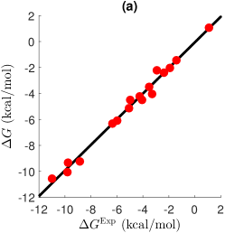
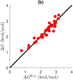
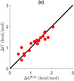
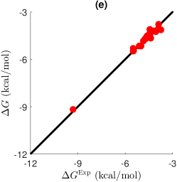
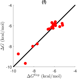
Figure 6: Comparison of $\mathbf{AVHL}$’s predicted and experiment solvation free energies for six groups. (a) SAMPL0, (b) alkene, (c) alkene, (d) ether, (e) alcohol, (f) phenol. In all charts, red circles for the predicted data, solid lines for the experiment data.

3.6 The best all around model for predicting the solvation free energy

Table 5: The RMS errors (in the unit of kcal/mol) for 26 models. The highlighted numbers indicate the best RMS error in a particular category.

Model$\backslash$ Group	SAMPL0	alkane	alkene	ether	alcohol	phenol
$\mathbf{A}$	2.27	0.40	0.35	0.84	0.57	0.59
$\mathbf{V}$	2.34	0.44	0.39	0.85	0.62	0.61
$\mathbf{L}$	1.07	0.29	0.34	0.23	0.28	0.55
$\mathbf{k}_{1}$	2.35	0.41	0.33	0.83	0.54	0.63
$\mathbf{k}_{2}$	2.32	0.40	0.33	0.81	0.52	0.59
$\mathbf{G}$	2.23	0.43	0.32	0.83	0.54	0.64
$\mathbf{H}$	2.34	0.41	0.33	0.81	0.51	0.61
$\mathbf{AL}$	0.45	0.23	0.20	0.23	0.28	0.54
$\mathbf{VL}$	1.06	0.28	0.33	0.19	0.18	0.44
$\mathbf{k}_{1}\mathbf{L}$	0.66	0.22	0.19	0.23	0.28	0.48
$\mathbf{k}_{2}\mathbf{L}$	0.65	0.23	0.23	0.22	0.28	0.54
$\mathbf{GL}$	0.52	0.23	0.18	0.23	0.28	0.47
$\mathbf{HL}$	0.43	0.23	0.24	0.22	0.28	0.53
$\mathbf{AVL}$	0.45	0.19	0.19	0.17	0.17	0.42
$\mathbf{Ak}_{1}\mathbf{L}$	0.36	0.22	0.19	0.22	0.28	0.46
$\mathbf{Ak}_{2}\mathbf{L}$	0.45	0.23	0.19	0.12	0.19	0.53
$\mathbf{AGL}$	0.31	0.23	0.19	0.23	0.27	0.43
$\mathbf{AHL}$	0.36	0.22	0.18	0.14	0.18	0.53
$\mathbf{Vk}_{1}\mathbf{L}$	0.53	0.21	0.19	0.19	0.17	0.41
$\mathbf{Vk}_{2}\mathbf{L}$	0.50	0.19	0.20	0.18	0.17	0.42
$\mathbf{VGL}$	0.46	0.20	0.17	0.18	0.17	0.41
$\mathbf{VHL}$	0.40	0.20	0.22	0.19	0.18	0.41
$\mathbf{AVk}_{1}\mathbf{L}$	0.31	0.19	0.18	0.14	0.17	0.41
$\mathbf{AVk}_{2}\mathbf{L}$	0.45	0.18	0.19	0.12	0.16	0.42
$\mathbf{AVGL}$	0.28	0.19	0.17	0.14	0.17	0.41
$\mathbf{AVHL}$	0.35	0.18	0.18	0.11	0.15	0.41

Finally, we determine which model will have the best solvation free energy prediction in each group, and then which one will provide an good prediction on average. Table 5 lists all the RMS errors of 26 models over 6 groups including SAMPL0, alkane, alkene, ether, alcohol and phenol sets. These results again confirm the important role of Lennard-Jones potential in the accuracy of solvation energy prediction as other studies have noted ^{77, 78, 32, 75}. The RMS errors of model $\mathbf{L}$ for SAMPL0, alkane, alkene, ether, alcohol, and phenol sets are, respectively, $1.07$, $0.29$, $0.34$, $0.23$, $0.28$ and $0.55$. It is obvious that these predictions are still not the best performance in comparison to other work such as that in Ref. ³⁴. This is easy to apprehend because model $\mathbf{L}$ only consists of Lennard-Jones potential while that in our previous work ³⁴ includes surface area, volume and Lennard-Jones potential itself. While models lacking of Lennard-Jones potential usually perform poorly in solvation free energy prediction. Specially, for SAMPL0 the RMS errors of those models are larger than $2.0$. However, for the rest of the test sets, the RMS errors of models without Lennard-Jones potential are always under $0.85$. Especially, in alkene test set, model $\mathbf{G}$ delivers a better RMS error, 0.32, than that of model $\mathbf{L}$, 0.34. This is probably because hydrophobic compounds in alkane and alkene groups contain only carbon and hydrogen and are very uniform. Whereas other test sets contain oxygen or nitrogen that has strong vdW interactions ⁷⁵ and thus prefer the Lennard-Jones potential.

As expected, more quantities appearing in the nonpolar component will produce a better solvation prediction in general. Table 5 indicates that two-term models always outperform related single-term models. Similar patterns can be found for three-term models and four-term models. The best results at each level of modeling are highlighted in Table 5. On average, model $\mathbf{AVHL}$ produces the best RMS errors. Its RMS errors for six groups in the discussed order are 0.35, 0.18, 0.18, 0.11, 0.15, and 0.41, respectively. To demonstrate the accuracy of model $\mathbf{AVHL}$, Fig. 6 depicts its predicted and experimental solvation free energies for SAMPL0, alkane, alkene, ether, alcohol and phenol sets. Since the results of SAMPL0 has been reported in Table 4, in the supporting information we only list the data for alkane, alkene, ether, alcohol and phenol tests in Tables S1, S2, S3 and S4, respectively.

By a comparison with our earlier work ^{1, 34}, the current models yield better solvation predictions for all test sets. The earlier work ^{1, 34} employs model $\mathbf{AVL}$ and invokes sophisticated mathematical algorithms, such as differential geometry and constrained optimization. The present approach utilizes FRI based rigidity surfaces which are very simple, stable and robust. Additionally, as an intrinsic property of a protein ^{55, 57, 57}, flexibility plays an important role in the solvation process. The use FRI based rigidity surfaces enables us to build the flexibility feature in our solvation analysis. Consequently, many of the present two-term models, such as $\mathbf{AL}$, $\mathbf{GL}$ and $\mathbf{HL}$, are able to deliver better predictions on all test sets. The predictions of the present $\mathbf{AVL}$ model are much better than those of our earlier $\mathbf{AVL}$ model ³⁴.

Table 5 reveals that models involving various curvatures are able to deliver some of the best results at each level of modeling. For example, at the single-term level of modeling, the Gaussian curvature model, $\mathbf{G}$, gives rise to better prediction for the alkene set. At the two-term level of modeling, models $\mathbf{HL}$, $\mathbf{k}_{1}\mathbf{L}$ and $\mathbf{GL}$ provide the best predictions for SAMPL0, alkane and alkene sets, respectively. At three-term and four-term levels of modelings, most best predictions are generated by curvature based models. Since curvatures are calculated analytically in the rigidity surface representation ^{51, 52, 53}, the use of curvatures is very robust and simple in the present work, see Section 2.6. Therefore, the present work establishes curvature as a robust, efficient and powerful approach for solvation analysis and prediction.

3.7 Five-fold validation

Table 6: Training Errors (TRN. Err.) and Validation Errors (VAL. Err.) for five-fold cross validation. Errors are in the unit of kcal/mol.

	Group 1			Group 2			Group 3			Group 4			Group 5
	T. Err.	VAL. Err.		TRN. Err.	VAL. Err.		TRN. Err.	VAL. Err.		TRN. Err.	VAL. Err.		TRN. Err.	VAL. Err.
Alkane	0.19	0.19		0.17	0.24		0.18	0.23		0.18	0.23		0.19	0.15
Alkene	0.15	0.40		0.14	0.34		0.18	0.30		0.17	0.23		0.19	0.10
Ether	0.10	0.21		0.11	0.13		0.10	0.22		0.07	0.26		0.12	0.07
Alcohol	0.15	0.21		0.17	0.07		0.11	0.31		0.14	0.46		0.14	0.27
Phenol	0.39	0.57		0.39	0.67		0.32	0.86		0.44	0.32		0.33	0.97

To further estimate how accurately the models with optimized parameters perform in practice, we carry out 5-fold cross validation. In this evaluation, each group of molecules is partitioned into 5 sub-groups as uniformly as possible. Of 5 sub-groups, we leave out one sub-group and employ model AVHL for the rest four sub-groups of of molecules. The optimized parameters are then utilized for the left out sub-group. Table 6 lists training errors and validation errors. It is seen that these two errors are of the same level, indicating the present method performs well.

4 Conclusion

Solvation analysis is a fundamental issue in computational biophysics, chemistry and material science and has attracted much attention in the past two decades. Implicit solvent models that split the solvation free energy into polar and nonpolar contributions have been a main workhorse in solvation free energy prediction. While the Poisson-Boltzmann theory is a well established model for polar solvation energy prediction, there is no general consensus about what constitutes a good nonpolar component. This paper explores the impact of area, volume, curvature and Lennard-Jones potential to the accuracy of the solvation free energy prediction in conjugation with a Poisson-Boltzmann based polar solvation model. To this end, 26 models involving the presence of different quantities in the nonpolar component are systematically studies in the current work. Some of these models that consist of Gaussian curvature, mean curvature, minimum curvature or maximum curvature are first known to our knowledge.

In order to analytically evaluate molecular curvatures, we utilize rigidity surfaces ^{51, 52, 53} as the molecular surface representation. Since the use of the rigidity surface does not require a surface evolution as in previous approaches ^{1, 33, 34}, the algorithm for achieving parameter optimization in the nonpolar component is much simpler than that in our earlier work ³⁴. To benchmark our models, we employ the SAMPL0 test set with 17 molecules, alkane set with 35 molecules, alkene set with 19 molecules, ether set with 15 molecules, alcohol set with 23 molecules, and phenol set with 18 molecules.

We first carry out intensive correlation analysis. It is found that surface areas and surface enclosed volumes are highly correlated for the above mentioned molecules, whereas various curvatures are poorly correlated to surface areas. Therefore, curvatures are complementary to surface areas and surface enclosed volumes in solvation modeling. Nevertheless, for a given set of similar molecules, maximum, minimum, mean and Gaussian curvatures and Gaussian curvatures are highly correlated to each other and to surface areas.

Based on the correlation analysis, a total 26 nontrivial models are constructed and examined against 6 test sets of molecules. Numerous numerical experiments indicate that the Lennard-Jones potential is essential to the accuracy of solvation free energy prediction, especially for molecules involving strong van der Waals interactions or attractive dispersive effects. However, it is found that various curvatures are at least as useful as surface area and surface enclosed volume in nonpolar solvation modeling. Many curvature based models deliver some of the best solvation free energy predictions.

Supporting Information Available

Addition results for interested models and additional correlation analysis for various curvatures (filename: URL will be inserted by publisher).

This work was supported in part by NSF Grant IIS- 1302285 and MSU Center for Mathematical Molecular Biosciences Initiative.

References

- Chen et al. 2010 Chen, Z.; Baker, N. A.; Wei, G. W. Differential geometry based solvation models I: Eulerian formulation. J. Comput. Phys. 2010, 229, 8231–8258
- Chen et al. 2011 Chen, Z.; Baker, N. A.; Wei, G. W. Differential geometry based solvation models II: Lagrangian formulation. J. Math. Biol. 2011, 63, 1139– 1200
- Chen and Wei 2011 Chen, Z.; Wei, G. W. Differential geometry based solvation models III: Quantum formulation. J. Chem. Phys. 2011, 135, 194108
- Ponder and Case 2003 Ponder, J. W.; Case, D. A. Force fields for protein simulations. Advances in Protein Chemistry 2003, 66, 27–85
- Husowitz and Talanquer 2007 Husowitz, B.; Talanquer, V. Solvent density inhomogeneities and solvation free energies in supercritical diatomic fluids: A density functional approach. The Journal of Chemical Physics 2007, 126, 054508
- Marenich et al. 2008 Marenich, A. V.; Cramer, C. J.; Truhlar, D. G. Perspective on Foundations of Solvation Modeling: The Electrostatic Contribution to the Free Energy of Solvation. J.Chem.Theory Comput 2008, 4, 877–877
- Davis and McCammon 1990 Davis, M. E.; McCammon, J. A. Electrostatics in biomolecular structure and dynamics. Chemical Reviews 1990, 94, 509–21
- Roux and Simonson 1999 Roux, B.; Simonson, T. Implicit solvent models. Biophysical Chemistry 1999, 78, 1–20
- Sharp and Honig 1990 Sharp, K. A.; Honig, B. Electrostatic Interactions in Macromolecules - Theory and Applications. Annual Review of Biophysics and Biophysical Chemistry 1990, 19, 301–332
- Koehl 2006 Koehl, P. Electrostatics calculations: latest methodological advances. Current Opinion in Structural Biology 2006, 16, 142–51
- David et al. 2000 David, L.; Luo, R.; Gilson, M. K. Comparison of generalized Born and Poisson models: Energetics and dynamics of HIV protease. Journal of Computational Chemistry 2000, 21, 295–309
- Baker 2005 Baker, N. A. Improving implicit solvent simulations: a Poisson-centric view. Current Opinion in Structural Biology 2005, 15, 137–43
- Fogolari et al. 2002 Fogolari, F.; Brigo, A.; Molinari, H. The Poisson-Boltzmann equation for biomolecular electrostatics: a tool for structural biology. Journal of Molecular Recognition 2002, 15, 377–92
- Zhou et al. 2008 Zhou, Y. C.; Feig, M.; Wei, G. W. Highly accurate biomolecular electrostatics in continuum dielectric environments. Journal of Computational Chemistry 2008, 29, 87–97
- Bashford and Case 2000 Bashford, D.; Case, D. A. Generalized Born models of macromolecular solvation effects. Annual Review of Physical Chemistry 2000, 51, 129–152
- Dominy and Brooks 1999 Dominy, B. N.; Brooks, C. L., III Development of a generalized Born model parameterization for proteins and nucleic acids. Journal of Physical Chemistry B 1999, 103, 3765–3773
- Gallicchio et al. 2002 Gallicchio, E.; Zhang, L. Y.; Levy, R. M. The SGB/NP hydration free energy model based on the surface generalized Born solvent reaction field and novel nonpolar hydration free energy estimators. Journal of Computational Chemistry 2002, 23, 517–29
- Grant et al. 2007 Grant, J. A.; Pickup, B. T.; Sykes, M. T.; Kitchen, C. A.; Nicholls, A. The Gaussian Generalized Born model: application to small molecules. Physical Chemistry Chemical Physics 2007, 9, 4913–22
- Onufriev et al. 2002 Onufriev, A.; Case, D. A.; Bashford, D. Effective Born radii in the generalized Born approximation: the importance of being perfect. Journal of Computational Chemistry 2002, 23, 1297–304
- Tjong and Zhou 2007 Tjong, H.; Zhou, H. X. GBr6NL: A generalized Born method for accurately reproducing solvation energy of the nonlinear Poisson-Boltzmann equation. Journal of Chemical Physics 2007, 126, 195102
- Tsui and Case 2001 Tsui, V.; Case, D. A. Calculations of the Absolute Free Energies of Binding between RNA and Metal Ions Using Molecular Dynamics Simulations and Continuum Electrostatics. Journal of Physical Chemistry B 2001, 105, 11314–11325
- Beglov and Roux 1996 Beglov, D.; Roux, B. Solvation of complex molecules in a polar liquid: an integral equation theory. Journal of Chemical Physics 1996, 104, 8678–8689
- Netz and Orland 2000 Netz, R. R.; Orland, H. Beyond Poisson-Boltzmann: Fluctuation effects and correlation functions. European Physical Journal E 2000, 1, 203–14
- Swanson et al. 2004 Swanson, J. M. J.; Henchman, R. H.; McCammon, J. A. Revisiting Free Energy Calculations: A Theoretical Connection to MM/PBSA and Direct Calculation of the Association Free Energy. Biophysical Journal 2004, 86, 67–74
- Massova and Kollman 2000 Massova, I.; Kollman, P. A. Combined molecular mechanical and continuum solvent approach (MM-PBSA/GBSA) to predict ligand binding. Perspectives in drug discovery and design 2000, 18, 113–135
- Stillinger 1973 Stillinger, F. H. Structure in Aqueous Solutions of Nonpolar Solutes from the Standpoint of Scaled-Particle Theory. J. Solution Chem. 1973, 2, 141 – 158
- Pierotti 1976 Pierotti, R. A. A scaled particle theory of aqueous and nonaqeous solutions. Chemical Reviews 1976, 76, 717–726
- Lum et al. 1999 Lum, K.; Chandler, D.; Weeks, J. D. Hydrophobicity at small and large length scales. Journal of Physical Chemistry B 1999, 103, 4570–7
- Huang and Chandler 2000 Huang, D. M.; Chandler, D. Temperature and length scale dependence of hydrophobic effects and their possible implications for protein folding. Proceedings of the National Academy of Sciences 2000, 97, 8324–8327
- Gallicchio and Levy 2004 Gallicchio, E.; Levy, R. M. AGBNP: An analytic implicit solvent model suitable for molecular dynamics simulations and high-resolution modeling. Journal of Computational Chemistry 2004, 25, 479–499
- Choudhury and Pettitt 2005 Choudhury, N.; Pettitt, B. M. On the mechanism of hydrophobic association of nanoscopic solutes. Journal of the American Chemical Society 2005, 127, 3556–3567
- Wagoner and Baker 2006 Wagoner, J. A.; Baker, N. A. Assessing implicit models for nonpolar mean solvation forces: the importance of dispersion and volume terms. Proceedings of the National Academy of Sciences of the United States of America 2006, 103, 8331–6
- Chen et al. 2012 Chen, Z.; Zhao, S.; Chun, J.; Thomas, D. G.; Baker, N. A.; Bates, P. B.; Wei, G. W. Variational approach for nonpolar solvation analysis. Journal of Chemical Physics 2012, 137
- Wang and Wei 2015 Wang, B.; Wei, G. W. Parameter optimization in differential geometry based solvation models. Journal Chemical Physics 2015, 143, 134119
- Lee and Richards 1971 Lee, B.; Richards, F. M. The interpretation of protein structures: estimation of static accessibility. J Mol Biol 1971, 55, 379–400
- Richards 1977 Richards, F. M. Areas, Volumes, Packing, and Protein Structure. Annual Review of Biophysics and Bioengineering 1977, 6, 151–176
- Connolly 1983 Connolly, M. L. Analytical molecular surface calculation. Journal of Applied Crystallography 1983, 16, 548–558
- Sanner et al. 1996 Sanner, M. F.; Olson, A. J.; Spehner, J. C. Reduced surface: An efficient way to compute molecular surfaces. Biopolymers 1996, 38, 305–320
- Yu et al. 2007 Yu, S. N.; Geng, W. H.; Wei, G. W. Treatment of geometric singularities in implicit solvent models. Journal of Chemical Physics 2007, 126, 244108
- Yu and Wei 2007 Yu, S. N.; Wei, G. W. Three-dimensional matched interface and boundary (MIB) method for treating geometric singularities. J. Comput. Phys. 2007, 227, 602–632
- Zhou et al. 2006 Zhou, Y. C.; Zhao, S.; Feig, M.; Wei, G. W. High order matched interface and boundary method for elliptic equations with discontinuous coefficients and singular sources. J. Comput. Phys. 2006, 213, 1–30
- Grant and Pickup 1995 Grant, J.; Pickup, B. A Gaussian description of molecular shape. Journal of Physical Chemistry 1995, 99, 3503–3510
- Chen and Lu 2011 Chen, M.; Lu, B. TMSmesh: A Robust Method for Molecular Surface Mesh Generation Using a Trace Technique. J Chem. Theory and Comput. 2011, 7, 203–212
- Li et al. 2014 Li, L.; Li, C.; Alexov, E. On the Modeling of Polar Component of Solvation Energy using Smooth Gaussian-Based Dielectric Function. Journal of Theoretical and Computational Chemistry 2014, 13, 10.1142/S0219633614400021
- Wei et al. 2005 Wei, G. W.; Sun, Y. H.; Zhou, Y. C.; Feig, M. Molecular multiresolution surfaces. arXiv:math-ph/0511001v1 2005, 1 – 11
- Bates et al. 2006 Bates, P. W.; Wei, G. W.; Zhao, S. The minimal molecular surface. arXiv:q-bio/0610038v1 2006, [q-bio.BM]
- Bates et al. 2008 Bates, P. W.; Wei, G. W.; Zhao, S. Minimal molecular surfaces and their applications. Journal of Computational Chemistry 2008, 29, 380–91
- Wei 2010 Wei, G. W. Differential geometry based multiscale models. Bulletin of Mathematical Biology 2010, 72, 1562 – 1622
- Wei et al. 2012 Wei, G.-W.; Zheng, Q.; Chen, Z.; Xia, K. Variational multiscale models for charge transport. SIAM Review 2012, 54, 699 – 754
- Wei 2013 Wei, G.-W. Multiscale, multiphysics and multidomain models I: Basic theory. Journal of Theoretical and Computational Chemistry 2013, 12, 1341006
- Xia et al. 2013 Xia, K. L.; Opron, K.; Wei, G. W. Multiscale multiphysics and multidomain models — Flexibility and Rigidity. Journal of Chemical Physics 2013, 139, 194109
- Opron et al. 2014 Opron, K.; Xia, K. L.; Wei, G. W. Fast and anisotropic flexibility-rigidity index for protein flexibility and fluctuation analysis. Journal of Chemical Physics 2014, 140, 234105
- Opron et al. 2015 Opron, K.; Xia, K. L.; Wei, G. W. Communication: Capturing protein multiscale thermal fluctuations. Journal of Chemical Physics 2015, 142
- Xia et al. 2015 Xia, K. L.; Opron, K.; Wei, G. W. Multiscale Gaussian network model (mGNM) and multiscale anisotropic network model (mANM). Journal of Chemical Physics 2015,
- Alvarez-Garcia and Barril 2014 Alvarez-Garcia, D.; Barril, X. Relationship between Protein Flexibility and Binding: Lessons for Structure-Based Drug Design. Journal of Chemical Theory and Computation 2014, 10, 2608–2614
- Bu and Callaway 2011 Bu, Z.; Callaway, D. J. Proteins MOVE! Protein dynamics and long-range allostery in cell signaling. Advances in Protein Chemistry and Structural Biology 2011, 83, 163–221
- Marsh and Teichmann 2014 Marsh, J. A.; Teichmann, S. A. Protein Flexibility Facilitates Quaternary Structure Assembly and Evolution. PLoS Biol 2014, 12, e1001870
- Helfrich 1973 Helfrich, W. Elastic Properties of Lipid Bilayers: Theory and Possible Experiments. Zeitschrift für Naturforschung Teil C 1973, 28, 693 – 703
- Dzubiella et al. 2006 Dzubiella, J.; Swanson, J. M. J.; McCammon, J. A. Coupling Hydrophobicity, Dispersion, and Electrostatics in Continuum Solvent Models. Physical Review Letters 2006, 96, 087802
- Sharp et al. 1991 Sharp, K. A.; Nicholls, A.; Friedman, R.; Honig, B. Extracting hydrophobic free energies from experimental data: relationship to protein folding and theoretical models. Biochemistry 1991, 30, 9686–9697
- Jackson and Sternberg 1994 Jackson, R. M.; Sternberg, M. J. Application of scaled particle theory to model the hydrophobic effect: Implications for molecular association and protein stability. Protein engineering 1994, 7, 371–383
- Wei 2000 Wei, G. W. Wavelets generated by using discrete singular convolution kernels. Journal of Physics A: Mathematical and General 2000, 33, 8577 – 8596
- Grant et al. 2001 Grant, J. A.; Pickup, B. T.; Nicholls, A. A smooth permittivity function for Poisson-Boltzmann solvation methods. Journal of Computational Chemistry 2001, 22, 608–640
- Chen et al. 2011 Chen, D.; Chen, Z.; Chen, C.; Geng, W. H.; Wei, G. W. MIBPB: A software package for electrostatic analysis. J. Comput. Chem. 2011, 32, 657 – 670
- Geng and Wei 2011 Geng, W.; Wei, G. W. Multiscale molecular dynamics using the matched interface and boundary method. J Comput. Phys. 2011, 230, 435–457
- Zheng et al. 2012 Zheng, Q.; Yang, S. Y.; Wei, G. W. Molecular surface generation using PDE transform. International Journal for Numerical Methods in Biomedical Engineering 2012, 28, 291–316
- Tian and Zhao 2014 Tian, W. F.; Zhao, S. A fast ADI algorithm for geometric flow equations in biomolecular surface generations. International Journal for Numerical Methods in Biomedical Engineering 2014, 30, 490–516
- Soldea et al. 2006 Soldea, O.; Elber, G.; Rivlin, E. Global segmentation and curvature analysis of volumetric data sets using trivariate B-spline functions. IEEE Trans. on PAMI 2006, 28, 265 – 278
- Xia et al. 2014 Xia, K. L.; Feng, X.; Tong, Y. Y.; Wei, G. W. Multiscale geometric modeling of macromolecules I: Cartesian representation. Journal of Computational Physics 2014, 275, 912–936
- Kindlmann et al. 2003 Kindlmann, G.; Whitaker, R.; Tasdizen, T.; Möller, T. Curvature-based transfer functions for direct volume rendering: methods and applications. Proc. IEEE Visualization 2003,
- Grant and Boyd 2014 Grant, M.; Boyd, S. CVX: Matlab Software for Disciplined Convex Programming, version 2.1. \urlhttp://cvxr.com/cvx, 2014
- Nicholls et al. 2008 Nicholls, A.; Mobley, D. L.; Guthrie, J. P.; Chodera, J. D.; Bayly, C. I.; Cooper, M. D.; Pande, V. S. Predicting Small-Molecule Solvation Free Energies: An Informal Blind Test for Computational Chemistry. J. Med. Chem. 2008, 51, 769–799
- Mobley and Guthrie 2014 Mobley, D. L.; Guthrie, J. P. FreeSolv: a database of experimental and calculated hydration free energies, with input files. Journal of Computer-Aided Molecular Design 2014, 28, 711–720
- Jakalian et al. 2000 Jakalian, A.; Bush, B. L.; Jack, D. B.; Bayly, C. I. Fast, efficient generation of high-quality atomic charges. AM1-BCC model: I. Method. Journal of Computational Chemistry 2000, 21, 132–146
- Mobley et al. 2009 Mobley, D. L.; Bayly, C. I.; Cooper, M. D.; Shirts, M. R.; Dill, K. A. Small Molecule Hydration Free Energies in Explicit Solvent: An Extensive Test of Fixed-Charge Atomistic Simulations. Journal of Chemical Theory and Computation 2009, 5, 350–358
- Xia et al. 2015 Xia, K. L.; Feng, X.; Tong, Y. Y.; Wei, G. W. Persistent Homology for the quantitative prediction of fullerene stability. Journal of Computational Chemsitry 2015, 36, 408–422
- Ashbaugh et al. 1999 Ashbaugh, H. S.; Kaler, E. W.; Paulaitis, M. E. A “universal” surface area correlation for molecular hydrophobic phenomena. Journal of the American Chemical Society 1999, 121, 9243–9244
- Gallicchio et al. 2000 Gallicchio, E.; Kubo, M. M.; Levy, R. M. Enthalpy-Entropy and Cavity Decomposition of Alkane Hydration Free Energies: Numerical Results and Implications for Theories of Hydrophobic Solvation. Journal of Physical Chemistry B 2000, 104, 6271–6285