The adaptive Crouzeix-Raviart element method for convection-diffusion eigenvalue problems

Abstract :  The convection-diffusion eigenvalue problems are hot topics, and computational mathematics community and physics community are concerned about them in recent years. In this paper, we consider the a posteriori error analysis and the adaptive algorithm of the Crouzeix-Raviart nonconforming element method for the convection-diffusion eigenvalue problems. We give the corresponding a posteriori error estimators, and prove their reliability and efficiency. Finally, the numerical results validate the theoretical analysis and show that the algorithm presented in this paper is efficient.
Keywords :  convection-diffusion eigenvalue problems, the Crouzeix-Raviart element, a posteriori error analysis, adaptive algorithm
AMS subject classifications. 65N25, 65N30

1 Introduction

The convection-diffusion eigenvalue problems have a strong background in physics, such as the distribution of contaminated material in nuclear waste pollution. Thus, using finite element methods to solve convection-diffusion eigenvalue problems has attracted much attention of scholars. [1, 2, 3] discussed a posteriori error estimates and the adaptive algorithms, [4] an adaptive homotopy approach, [5, 6] extrapolation methods, [7] function value recovery algorithms, [8] spectral element methods, [9, 10] multilevel correction method, and so on. This paper aims at deriving the a posteriori error estimators and the adaptive algorithm of the Crouzeix-Raviart element(C-R element) methods for the convection-diffusion eigenvalue problems.
The adaptive finite element method is a mainstream in scientific computing (see [11, 12, 13, 14]). In past years, the research of the a posteriori error and the adaptive algorithm of convection-diffusion eigenvalue problems used to adopt the conforming finite element methods(see[3, 8, 12]). [15] and [16] discussed a posteriori error estimate of the nonconforming methods for Laplace equation and Laplace eigenvalue problem, respectively. Based on the study of [15, 16], this paper first discusses the nonconforming finite element adaptive method for convection-diffusion eigenvalue problems. We give the a posteriori error estimators and prove their reliability and efficiency, and give the adaptive algorithm. Finally we use some numerical examples to verify our theoretical results.
In this paper, $C$ is a positive constant independent of $h$, which may not be the same constant in different places. For simplicity, we use symbol $a\lesssim b$ to replace $a\leq Cb$. The notation $a\approx b$ abbreviates $a\lesssim b\lesssim a$.

2 Preliminaries

Consider the following convection-diffusion eigenvalue problem:

$$-\Delta u+\mathbf{b}\cdot\nabla u=\lambda u~{}~{}~{}in~{}\Omega,~{}~{}~{}~{}~{}u=0~{}~{}~{}on~{}\partial\Omega,$$ (2.1)

where $\Omega\subset\mathbb{R}^{2}$ is a polygon bounded domain with boundary $\partial\Omega$.
Let

$$a(u,v)=\int_{\Omega}\nabla u\cdot\nabla\overline{v}+\mathbf{b}\cdot\nabla u\overline{v}~{}dx,~{}~{}~{}~{}~{}b(u,v)=\int_{\Omega}u\overline{v}dx.$$ (2.2)

The variational problem associated with (2.1) is given by: Find $(\lambda,u)\in\mathbb{C}\times H_{0}^{1}(\Omega)$, $\parallel u\parallel_{L^{2}(\Omega)}=1,$ such that

$$a(u,v)=\lambda b(u,v),~{}~{}~{}\forall v\in H_{0}^{1}(\Omega).$$ (2.3)

Let $\mathcal{T}_{h}=\{K\}$ be a regular triangular mesh of $\Omega$.
Let $V_{h}$ denote the Crouzeix-Raviart nonconforming finite element space over $\mathcal{T}_{h}$. Then, the C-R element approximation of (2.3) is given as follows: Find $(\lambda_{h},u_{h})\in\mathbb{C}\times V_{h}$, $\parallel u_{h}\parallel_{L^{2}(\Omega)}=1$, such that

$$a_{h}(u_{h},v)=\lambda_{h}b(u_{h},v),~{}~{}~{}\forall v\in V_{h}.$$ (2.4)

where

$$a_{h}(u_{h},v)=\sum\limits_{K}\int_{K}\nabla_{h}u_{h}\nabla\overline{v}+\mathbf{b}\cdot\nabla_{h}u_{h}\overline{v}dx.$$ (2.5)

Since the discrete space $V_{h}$ is nonconforming, we regard $\nabla_{h}$ as the gradient operator which is defined elementwise.
The dual problem of (2.1) is as below:

$$-\Delta u^{*}-\nabla\cdot(\overline{\mathbf{b}}u^{*})=\lambda^{*}u^{*}~{}~{}~{}in~{}\Omega,~{}~{}~{}~{}~{}u^{*}=0~{}~{}~{}on~{}\partial\Omega.$$ (2.6)

The corresponding variational form of (2.6) is as follows: Find $(\lambda^{*},u^{*})\in\mathbb{C}\times H_{0}^{1}(\Omega)$, $\parallel u^{*}\parallel_{L^{2}(\Omega)}=1$, such that

$$a(v,u^{*})=\overline{\lambda^{*}}b(v,u^{*}),~{}~{}~{}\forall v\in H_{0}^{1}(\Omega),$$ (2.7)

where

$$a(v,u^{*})=\int_{\Omega}\nabla v\cdot{\nabla\overline{u^{*}}}+\nabla v\cdot{\mathbf{b}\overline{u^{*}}}dx,~{}~{}~{}b(v,u^{*})=\int_{\Omega}v\overline{u^{*}}dx.$$ (2.8)

Then the C-R element approximation of (2.7) is as below: Find $(\lambda_{h}^{*},u_{h}^{*})\in\mathbb{C}\times V_{h}$, $\parallel u_{h}^{*}\parallel_{L^{2}(\Omega)}=1$, such that

$$a_{h}(v,u_{h}^{*},)=\overline{\lambda_{h}^{*}}b(v,u_{h}^{*}),~{}~{}~{}\forall v\in V_{h},$$ (2.9)

where

$$a_{h}(v,u_{h}^{*})=\sum\limits_{T}\int_{T}\nabla v\nabla\overline{u_{h}^{*}}+\nabla v\cdot\mathbf{b}\overline{u_{h}^{*}}dx,~{}~{}~{}b(v,u_{h}^{*})=\int_{\Omega}v\overline{u_{h}^{*}}dx.$$ (2.10)

[17] discusses the non-conforming finite element approximation, and proves the error estimates of the discrete eigenvalues obtained by the Adini element, Morley-Zienkiewicz element et. al. Due to the reference [17], we can deduce the following Lemma.

Lemma 2.1.

For the C-R nonconforming finite element methods of problem (2.1) and (2.6), the a priori error estimates are given:

$$\parallel\nabla_{h}(u-u_{h})\parallel_{L^{2}(\Omega)}\lesssim h^{r},$$ (2.11)

$$\parallel u-u_{h}\parallel_{L^{2}(\Omega)}\lesssim h^{r}\parallel\nabla_{h}(u-u_{h})\parallel_{L^{2}(\Omega)},$$ (2.12)

$$\parallel\nabla_{h}(u^{*}-u_{h}^{*})\parallel_{L^{2}(\Omega)}\lesssim h^{\frac{r}{\alpha}},$$ (2.13)

$$\parallel u^{*}-u_{h}^{*}\parallel_{L^{2}(\Omega)}\lesssim(h^{r}\parallel\nabla_{h}(u^{*}-u_{h}^{*})\parallel_{L^{2}(\Omega)})^{\frac{1}{\alpha}},$$ (2.14)

$$\mid\lambda-\lambda_{h}\mid\lesssim\parallel\nabla_{h}(u-u_{h})\parallel_{L^{2}(\Omega)}\cdot\parallel\nabla_{h}(u^{*}-u_{h}^{*})\parallel_{L^{2}(\Omega)}.$$ (2.15)

Owing to the above conclusions, we can get the following estimate: there exist some positive constants $0<\beta<1$ and $h_{0}>0$ (when $h<h_{0}$) with

$$\mid\lambda-\lambda_{h}\mid\parallel u\parallel_{L^{2}(\Omega)}+\mid\lambda_{h}\mid\parallel u-u_{h}\parallel_{L^{2}(\Omega)}+\parallel u-u_{h}\parallel_{L^{2}(\Omega)}$$

$$~{}~{}~{}\leq\beta\parallel\nabla_{h}(u-u_{h})\parallel_{L^{2}(\Omega)}.$$ (2.16)

3 A posteriori error analysis

Now we introduce some symbols for reading convenience. Suppose $K$ is one given element of $\mathcal{T}_{h}$, and $h_{K}$ represents the diameter of $K$. We use $\varepsilon$ to denote the set of all edges in $\mathcal{T}_{h}$, $\varepsilon(\Omega)$ the set of interior edges and $\varepsilon(K)$ the set of edges of the element $K$, respectively. For any given edge $E\in\mathcal{\varepsilon}(\Omega)$ with length $h_{E}=|E|$, we assign the fixed unit normal $\nu_{E}:=(\nu_{1},\nu_{2})$ and tangential vector $\tau_{E}:=(-\nu_{2},\nu_{1})$. Once $\nu_{E}$ and $\tau_{E}$ have been fixed on $E$, in relation to $\nu_{E}$ one defines the elements $K_{-}\in\mathcal{T}_{h}$ and $K_{+}\in\mathcal{T}_{h}$, with $E=K_{+}\bigcap K_{-}$ and $\omega_{E}=K_{+}\bigcup K_{-}$. Given $E\in\varepsilon(\Omega)$, we denote by $[v]:=(v|_{K_{+}})|_{E}-(v|_{K_{-}})|_{E}$ the jump of some $R^{d}$-valued function $v$ defined in $\Omega$ across $E$ with $d=1,2$. And throughout this paper, $[\cdot]$ denotes the jump of the piecewise smooth function across the internal edge $E$, and the trace for the boundary edge $E$.
Define the a posteriori error estimators on the element $K$ as below:

$$\eta_{h,K}:=(h_{K}^{2}\parallel\lambda_{h}u_{h}+\Delta_{h}u_{h}-\mathbf{b}\cdot\nabla_{h}u_{h}\parallel_{L^{2}(K)}^{2})^{\frac{1}{2}},$$

$$\eta_{h,K}^{*}:=(h_{K}^{2}\parallel\lambda_{h}^{*}u_{h}^{*}+\Delta_{h}u_{h}^{*}+\nabla_{h}\cdot\mathbf{b}u_{h}^{*}\parallel_{L^{2}(K)}^{2})^{\frac{1}{2}},$$

$$\eta_{h,K,\nu_{E}}:=(\frac{1}{2}\sum_{E\in\partial K}h_{E}\parallel[\nabla_{h}u_{h}]\cdot\nu_{E}\parallel_{L^{2}(E)}^{2})^{\frac{1}{2}},$$

$$\eta_{h,K,\nu_{E}}^{*}:=(\frac{1}{2}\sum_{E\in\partial K}h_{E}\parallel[\nabla_{h}u_{h}^{*}+\mathbf{b}u_{h}^{*}]\cdot\nu_{E}\parallel_{L^{2}(E)}^{2})^{\frac{1}{2}},$$

$$\eta_{h,K,\tau_{E}}:=(\frac{1}{2}\sum_{E\in\partial K}h_{E}\parallel[\nabla_{h}u_{h}]\cdot\tau_{E}\parallel_{L^{2}(E)}^{2})^{\frac{1}{2}},$$

$$\eta_{h,K,\tau_{E}}^{*}:=(\frac{1}{2}\sum_{E\in\partial K}h_{E}\parallel[\nabla_{h}u_{h}^{*}+\mathbf{b}u_{h}^{*}]\cdot\tau_{E}\parallel_{L^{2}(E)}^{2})^{\frac{1}{2}},$$

and the residual sum on $K$ are given by

$$\eta_{h}(K)^{2}:=\eta_{h,K}^{2}+\sum_{E\in\varepsilon(K),E\not\subset\partial\Omega}\eta_{h,K,\nu_{E}}^{2}+\sum_{E\in\varepsilon(K)}\eta_{h,K,\tau_{E}}^{2},$$ (3.1)

$$\eta_{h}^{*}(K)^{2}:=(\eta_{h,K}^{*})^{2}+\sum_{E\in\varepsilon(K),E\not\subset\partial\Omega}(\eta_{h,K,\nu_{E}}^{*})^{2}+\sum_{E\in\varepsilon(K)}(\eta_{h,K,\tau_{E}}^{*})^{2}.$$ (3.2)

For any $\mathcal{M}_{h}\subset\mathcal{T}_{h}$, define the estimators over $\mathcal{M}_{h}$ by

$$\eta_{h}(\mathcal{M}_{h})^{2}:=\sum_{K\in\mathcal{M}_{h}}\eta_{h}(K)^{2},~{}~{}~{}\eta_{h}^{*}(\mathcal{M}_{h})^{2}:=\sum_{K\in\mathcal{M}_{h}}\eta_{h}^{*}(K)^{2}.$$ (3.3)

The left parts of this section aim at proving the reliability and the efficiency of the estimators $\eta_{h}(\mathcal{T}_{h})$ and $\eta_{h}^{*}(\mathcal{T}_{h})$. The reliability of the estimators are based on the following lemma (see[14, 16]).

Lemma 3.1.

Under the assumption (2) there holds

$$|a_{h}(u-u_{h},u-u_{h})|\lesssim\min_{v\in H_{0}^{1}(\Omega)}\parallel\nabla_{h}(u_{h}-v)\parallel_{L^{2}(\Omega)}^{2}$$

$$~{}~{}~{}~{}~{}~{}+\sup_{w\in H_{0}^{1}(\Omega)}\frac{|b(\lambda_{h}u_{h},w)-a_{h}(u_{h},w)|}{\parallel w\parallel_{L^{2}(\Omega)}}\parallel\nabla(u-v)\parallel_{L^{2}(\Omega)},$$ (3.4)

where $(\lambda,u)\in\mathbb{C}\times H_{0}^{1}(\Omega)$ and $(\lambda_{h},u_{h})\in\mathbb{C}\times V_{h}$ are the solutions to problems(2.3)and(2.4), respectively. For the dual problem, it is similar:

$$|a_{h}(u^{*}-u_{h}^{*},u^{*}-u_{h}^{*})|\lesssim\min_{v\in H_{0}^{1}(\Omega)}\parallel\nabla_{h}(u_{h}^{*}-v)\parallel_{L^{2}(\Omega)}^{2}$$

$$~{}~{}~{}~{}~{}~{}+\sup_{w\in H_{0}^{1}(\Omega)}\frac{|b(\lambda_{h}^{*}u_{h}^{*},w)-a_{h}(u_{h}^{*},w)|}{\parallel w\parallel_{L^{2}(\Omega)}}\parallel\nabla(u^{*}-v)\parallel_{L^{2}(\Omega)}.$$ (3.5)

Proof. For any $v\in H_{0}^{1}(\Omega)$,

$$|a_{h}(u-u_{h},u-u_{h})|=|a_{h}(u-u_{h},u-v+v-u_{h})|$$

$$~{}~{}~{}=|a(u,u-v)-a_{h}(u_{h},u-v)+a_{h}(u-u_{h},v-u_{h})|$$

$$~{}~{}~{}=|b(\lambda u-\lambda_{h}u+\lambda_{h}u-\lambda_{h}u_{h},u-u_{h}+u_{h}-v)+b(\lambda_{h}u_{h},u-v)$$

$$~{}~{}+a_{h}(u-u_{h},v-u_{h})-a_{h}(u_{h},u-v)|$$

$$~{}~{}~{}\leq|b((\lambda-\lambda_{h})u,u-u_{h})+b(\lambda_{h}(u-u_{h}),u-u_{h})|$$

$$~{}~{}~{}~{}~{}~{}+|b((\lambda-\lambda_{h})u,v-u_{h})+b(\lambda_{h}(u-u_{h}),v-u_{h})|$$

$$~{}~{}~{}+|a_{h}(u-u_{h},v-u_{h})|$$

$$~{}~{}~{}+|b(\lambda_{h}u_{h},u-v)-a_{h}(u_{h},u-v)|.$$ (3.6)

Due to (2), we can get

$$|b((\lambda-\lambda_{h})u,u-u_{h})+b(\lambda_{h}(u-u_{h}),u-u_{h})|$$

$$~{}~{}~{}\lesssim(\mid\lambda-\lambda_{h}\mid\parallel u\parallel_{L^{2}(\Omega)}+\mid\lambda_{h}\mid\parallel u-u_{h}\parallel_{L^{2}(\Omega)})\parallel u-u_{h}\parallel_{L^{2}(\Omega)}$$

$$~{}~{}~{}\leq\beta^{2}\parallel\nabla_{h}(u-u_{h})\parallel_{L^{2}(\Omega)}^{2}.$$ (3.7)

$$|b((\lambda-\lambda_{h})u,v-u_{h})+b(\lambda_{h}(u-u_{h}),v-u_{h})|$$

$$~{}~{}~{}\lesssim(\mid\lambda-\lambda_{h}\mid\parallel u\parallel_{L^{2}(\Omega)}+\mid\lambda_{h}\mid\parallel u-u_{h}\parallel_{L^{2}(\Omega)})\parallel v-u_{h}\parallel_{L^{2}(\Omega)}$$

$$~{}~{}~{}\leq\beta\parallel\nabla_{h}(u-u_{h})\parallel_{L^{2}(\Omega)}\parallel v-u_{h}\parallel_{L^{2}(\Omega)}.$$ (3.8)

Using the Young and Poincar$\acute{e}$ inequalities, we obtain

$$~{}\beta\parallel\nabla_{h}(u-u_{h})\parallel_{L^{2}(\Omega)}\parallel v-u_{h}\parallel_{L^{2}(\Omega)}$$

$$~{}\leq\frac{1}{2}(\varepsilon^{2}\beta^{2}\parallel\nabla_{h}(u-u_{h})\parallel_{L^{2}(\Omega)}^{2}+\frac{1}{\varepsilon^{2}}\parallel v-u_{h}\parallel^{2}_{L^{2}(\Omega)})$$

$$~{}\leq\frac{1}{2}(\varepsilon^{2}\beta^{2}\parallel\nabla_{h}(u-u_{h})\parallel_{L^{2}(\Omega)}^{2}+\frac{C1}{\varepsilon^{2}}\parallel\nabla_{h}(v-u_{h})\parallel^{2}_{L^{2}(\Omega)}).$$ (3.9)

The inequality (3) gives

$$~{}~{}~{}|a_{h}(u-u_{h},v-u_{h})|$$

$$=|\sum\limits_{K}\int_{K}\nabla_{h}(u-u_{h})\cdot\nabla_{h}\overline{(v-u_{h})}+\mathbf{b}\cdot\nabla_{h}(u-u_{h})\overline{(v-u_{h})}dx|$$

$$\lesssim\sum\limits_{K}\{\parallel\nabla_{h}(u-u_{h})\parallel_{L^{2}(K)}\parallel\nabla_{h}(v-u_{h})\parallel_{L^{2}(K)}$$

$$~{}~{}~{}+\mid\mathbf{b}\mid\parallel\nabla_{h}(u-u_{h})\parallel_{L^{2}(K)}\parallel(v-u_{h})\parallel_{L^{2}(K)}\}$$

$$\lesssim\parallel\nabla_{h}(u-u_{h})\parallel_{L^{2}(\Omega)}\parallel\nabla_{h}(v-u_{h})\parallel_{L^{2}(\Omega)}$$

$$\leq(\frac{1}{2}(\varepsilon^{2}\parallel\nabla_{h}(u-u_{h})\parallel_{L^{2}(\Omega)}^{2}+\frac{1}{\varepsilon^{2}}\parallel v-u_{h}\parallel^{2}_{L^{2}(\Omega)})$$

$$\leq(\frac{1}{2}(\varepsilon^{2}\parallel\nabla_{h}(u-u_{h})\parallel_{L^{2}(\Omega)}^{2}+\frac{C2}{\varepsilon^{2}}\parallel\nabla_{h}(v-u_{h})\parallel^{2}_{L^{2}(\Omega)}).$$ (3.10)

Combining (3), (3), (3) with (3), we obtain from (3)

$$|a_{h}(u-u_{h},u-u_{h})|\leq(\frac{1}{2}\varepsilon^{2}\beta^{2}+\beta^{2}+\frac{C1}{2}\varepsilon^{2})\parallel\nabla_{h}(u-u_{h})\parallel_{L^{2}(\Omega)}^{2}$$

$$~{}~{}~{}~{}~{}~{}+(\frac{1}{2\varepsilon^{2}}+\frac{C2}{2\varepsilon^{2}})\parallel\nabla_{h}(u_{h}-v)\parallel_{L^{2}(\Omega)}^{2}+|b(\lambda_{h}u_{h},u-v)-a_{h}(u_{h},u-v)|,$$

then, we have

$$~{}~{}~{}|a_{h}(u-u_{h},u-u_{h})|$$

$$\lesssim\parallel\nabla_{h}(u_{h}-v)\parallel_{L^{2}(\Omega)}^{2}+|b(\lambda_{h}u_{h},u-v)-a_{h}(u_{h},u-v)|$$

$$\lesssim\parallel\nabla_{h}(u_{h}-v)\parallel_{L^{2}(\Omega)}^{2}$$

$$~{}~{}~{}+\frac{|b(\lambda_{h}u_{h},u-v)-a_{h}(u_{h},u-v)|}{\parallel\nabla(u-v)\parallel_{L^{2}(\Omega)}}\parallel\nabla(u-v)\parallel_{L^{2}(\Omega)}$$

$$\lesssim\min_{v\in H_{0}^{1}(\Omega)}\parallel\nabla_{h}(u_{h}-v)\parallel_{L^{2}(\Omega)}^{2}$$

$$~{}~{}~{}+\sup_{w\in H_{0}^{1}(\Omega)}\frac{|b(\lambda_{h}u_{h},w)-a_{h}(u_{h},w)|}{\parallel w\parallel_{L^{2}(\Omega)}}\parallel\nabla(u-v)\parallel_{L^{2}(\Omega)}.$$ (3.11)

Then the proof of (3.1) is finished, and the proof of (3.1) is similar.  $\Box$

Based on the work of [16, 18], we have the following Lemma:

Lemma 3.2.

The following estimate is valid:

$$\min_{v\in H_{0}^{1}(\Omega)}{\parallel\nabla_{h}(u_{h}-v)\parallel}^{2}_{L^{2}(\Omega)}\lesssim\sum_{E\in\varepsilon}h_{E}\parallel[\nabla_{h}u_{h}]\cdot\tau_{E}\parallel_{L^{2}(E)}^{2}.$$ (3.12)

Let $S_{0}^{1}(\mathcal{T}_{h})$ denote the elementwise linear conforming finite element space over $\mathcal{T}_{h}$. For the analysis in the rear, we need the $\mathrm{Cl\acute{e}ment-type}$ interpolation operator $\mathcal{L}:H_{0}^{1}(\Omega)\mapsto S_{0}^{1}(\mathcal{T}_{h})$ with the properties(see[20, 21, 22])

$$\parallel\nabla\mathcal{L}\varphi\parallel_{L^{2}(K)}+\parallel h_{K}^{-1}(\varphi-\mathcal{L}\varphi)\parallel_{L^{2}(K)}\lesssim\parallel\nabla\varphi\parallel_{L^{2}(\omega_{K})},$$ (3.13)

and

$$\parallel h_{E}^{\frac{-1}{2}}(\varphi-\mathcal{L}\varphi)\parallel_{L^{2}(E)}\lesssim\parallel\nabla\varphi\parallel_{L^{2}(\omega_{K})},$$ (3.14)

where $E\in\mathcal{\varepsilon}(K)$ and $\varphi\in H_{0}^{1}(\Omega)$. In this paper, $\omega_{K}$ denotes the element patch defined as

$$\omega_{K}:=\{{T\in\mathcal{T}_{h}:\overline{T}\bigcap\overline{K}\neq\emptyset}\}.$$ (3.15)

Refering to [16], we can prove the following Lemma.

Lemma 3.3.

The following estimates are valid:

$$\sup_{w\in H_{0}^{1}(\Omega)}\frac{|b(\lambda_{h}u_{h},w)-a_{h}(u_{h},w)|}{\parallel\nabla w\parallel_{L^{2}(\Omega)}}\lesssim(\sum\limits_{K\in\mathcal{T}_{h}}\eta_{h,K}^{2}+\sum_{E\in\varepsilon(\Omega)}\eta_{h,K,\nu_{E}}^{2})^{\frac{1}{2}},$$ (3.16)

$$\sup_{w\in H_{0}^{1}(\Omega)}\frac{|b(w,\lambda_{h}^{*}u_{h}^{*})-a_{h}(w,u_{h}^{*})|}{\parallel\nabla w\parallel_{L^{2}(\Omega)}}\lesssim(\sum\limits_{K\in\mathcal{T}_{h}}(\eta_{h,K}^{*})^{2}+\sum_{E\in\varepsilon(\Omega)}(\eta_{h,K,\nu_{E}}^{*})^{2})^{\frac{1}{2}}.$$ (3.17)

Proof. Using the estimates (3.13) and (3.14) and integrating by parts, we can deduce that

$$\mid b(\lambda_{h}u_{h},w)-a_{h}(u_{h},w)\mid=|(\lambda_{h}u_{h},w-\mathcal{L}w)_{L^{2}(\Omega)}-a_{h}(u_{h},w-\mathcal{L}w)_{L^{2}(\Omega)}|$$

$$~{}~{}~{}=|\sum_{K}\int_{K}\lambda_{h}u_{h}\overline{(w-\mathcal{L}w)}dx-\sum_{K}\int_{K}-\Delta_{h}u_{h}\overline{(w-\mathcal{L}w)}$$

$$~{}~{}~{}~{}~{}~{}+\mathbf{b}\cdot\nabla_{h}u_{h}\overline{(w-\mathcal{L}w)}dx-\int_{\partial k}\frac{\partial u_{h}}{\partial\nu}\overline{(w-\mathcal{L}w)}ds|$$

$$~{}~{}~{}=|\sum_{K}\int_{K}(\lambda_{h}u_{h}+\Delta_{h}u_{h}-\mathbf{b}\cdot\nabla_{h}u_{h})\overline{(w-\mathcal{L}w)}dx-\sum_{K}\int_{\partial k}\frac{\partial u_{h}}{\partial\nu}\overline{(w-\mathcal{L}w)}ds|$$

$$\lesssim\sum_{K}\parallel\lambda_{h}u_{h}+\Delta_{h}u_{h}-\mathbf{b}\cdot\nabla_{h}u_{h}\parallel_{L^{2}(K)}\cdot h_{K}\parallel\nabla w\parallel_{L^{2}(\omega_{K})}$$

$$~{}~{}~{}~{}~{}~{}~{}~{}~{}+\sum_{E\in\varepsilon(\Omega)}\parallel\nabla_{h}u_{h}\cdot\nu_{E}\parallel_{L^{2}(E)}\cdot h_{E}^{\frac{1}{2}}\parallel\nabla w\parallel_{L^{2}(\omega_{K})}$$

$$\lesssim(\sum_{K}h_{K}^{2}\parallel\lambda_{h}u_{h}+\Delta_{h}u_{h}-\mathbf{b}\cdot\nabla_{h}u_{h}\parallel_{L^{2}(K)}^{2})^{\frac{1}{2}}(\sum_{K}\parallel\nabla w\parallel_{L^{2}(\omega_{K})}^{2})^{\frac{1}{2}}$$

$$~{}~{}~{}~{}~{}~{}~{}~{}~{}+(\sum_{E\in\varepsilon(\Omega)}h_{E}\parallel\nabla_{h}u_{h}\cdot\nu_{E}\parallel_{L^{2}(E)}^{2})^{\frac{1}{2}}(\sum_{E\in\varepsilon(\Omega)}\parallel\nabla w\parallel_{L^{2}(\omega_{K})}^{2})^{\frac{1}{2}}$$

$$\lesssim(\sum_{K}h_{K}^{2}\parallel\lambda_{h}u_{h}+\Delta_{h}u_{h}-\mathbf{b}\cdot\nabla_{h}u_{h}\parallel_{L^{2}(K)}^{2}$$

$$~{}~{}~{}~{}~{}~{}~{}~{}~{}+\sum_{E\in\varepsilon(\Omega)}h_{E}\parallel[\nabla_{h}u_{h}]\cdot\nu_{E}\parallel_{L^{2}(E)}^{2})^{\frac{1}{2}}\parallel\nabla w\parallel_{L^{2}(\Omega)}$$

$$\lesssim(\sum\limits_{K\in\mathcal{T}_{h}}\eta_{h,K}^{2}+\sum_{E\in\varepsilon(\Omega)}\eta_{h,K,\nu_{E}}^{2})^{\frac{1}{2}}\parallel\nabla w\parallel_{L^{2}(\Omega)}.$$ (3.18)

This ends the proof. The proof of (3.17) is similar.  $\Box$

Combining Lemma 3.2 with Lemma 3.3, we can get the reliability of the a posteriori error estimators.

Theorem 3.1.

Let $(\lambda,u)\in\mathbb{C}\times H_{0}^{1}(\Omega)$ and $(\lambda_{h},u_{h})\in\mathbb{C}\times V_{h}$ be the solutions to problems (2.3) and (2.4), and let $(\lambda^{*},u^{*})\in\mathbb{C}\times H_{0}^{1}(\Omega)$ and $(\lambda_{h}^{*},u_{h}^{*})\in\mathbb{C}\times V_{h}$ be the solutions to problems(2.7) and(2.9), respectively. Under the assumption (2) there holds

$$\|u-u_{h}\|_{h}^{2}\lesssim\eta_{h}(\mathcal{T}_{h})^{2},$$ (3.19)

$$\|u^{*}-u_{h}^{*}\|_{h}^{2}\lesssim\eta_{h}^{*}(\mathcal{T}_{h})^{2},$$ (3.21)

$$|\lambda-\lambda_{h}|\lesssim\eta_{h}(\mathcal{T}_{h})^{2}+\eta_{h}^{*}(\mathcal{T}_{h})^{2}.$$

Proof. Combining Lemmas 3.1-3.3 we get (3.19) and (3.21). Substituting (3.19) and (3.21) into (2.15) yields (3.21).  $\Box$

Next, we shall prove the efficiency of the a posteriori error estimators.

Theorem 3.2.

Assume the conditions of Theorem 3.1 hold, then

$$\eta_{h}(\mathcal{T}_{h})^{2}\lesssim\|u-u_{h}\|_{h}^{2},$$ (3.22)

$$\eta_{h}^{*}(\mathcal{T}_{h})^{2}\lesssim\|u^{*}-u_{h}^{*}\|_{h}^{2}.$$ (3.23)

Proof. 1. Proof of $\sum\limits_{K\in\mathcal{T}_{h}}\eta_{h,K}^{2}\lesssim\parallel\nabla(u-u_{h})\parallel_{L^{2}(\Omega)}^{2}$
  Given $K\in\mathcal{T}_{h}$, let $b_{K}=27\lambda_{1}\lambda_{2}\lambda_{3}$ with $\lambda_{i}$, $i=1,2,3$. Define

$$v_{K}=b_{K}(\lambda_{h}u_{h}+\Delta_{h}u_{h}-\mathbf{b}\cdot\nabla_{h}u_{h})$$ (3.24)

Then, we have

$$\parallel\lambda_{h}u_{h}+\Delta_{h}u_{h}-\mathbf{b}\cdot\nabla_{h}u_{h}\parallel_{L^{2}(K)}^{2}\approx(\lambda_{h}u_{h}+\Delta_{h}u_{h}-\mathbf{b}\cdot\nabla_{h}u_{h},v_{K})_{L^{2}(K)}$$

$$~{}~{}~{}=(\lambda_{h}u_{h}-\lambda u+\lambda u+\Delta_{h}u_{h}-\mathbf{b}\cdot\nabla_{h}u_{h},v_{K})_{L^{2}(K)}$$

$$~{}~{}~{}=(\lambda_{h}u_{h}-\lambda u,v_{K})_{L^{2}(K)}+(-\Delta u+\mathbf{b}\cdot\nabla u+\Delta_{h}u_{h}-\mathbf{b}\cdot\nabla_{h}u_{h},v_{K})_{L^{2}(K)}$$

$$~{}~{}~{}=(\lambda_{h}u_{h}-\lambda u,v_{K})_{L^{2}(K)}+(-\Delta u+\Delta_{h}u_{h},v_{K})_{L^{2}(K)}$$

$$~{}~{}~{}~{}~{}~{}+(\mathbf{b}\cdot\nabla u-\mathbf{b}\cdot\nabla_{h}u_{h},v_{K})_{L^{2}(K)}$$

$$~{}~{}~{}=(\lambda_{h}u_{h}-\lambda u,v_{K})_{L^{2}(K)}+(\nabla_{h}(u-u_{h}),\nabla v_{K})_{L^{2}(K)}$$

$$~{}~{}~{}~{}~{}~{}+(\mathbf{b}\cdot\nabla u-\mathbf{b}\cdot\nabla_{h}u_{h},v_{K})_{L^{2}(K)}.$$ (3.25)

Using the Young inequalities in (3) to obtain

$$|(\lambda_{h}u_{h}-\lambda u,v_{K})_{L^{2}(K)}|\leq\parallel\lambda_{h}u_{h}-\lambda u\parallel_{L^{2}(K)}\parallel v_{K}\parallel_{L^{2}(K)}$$

$$~{}~{}~{}\lesssim\parallel\lambda_{h}u_{h}-\lambda u\parallel_{L^{2}(K)}\parallel\lambda_{h}u_{h}+\Delta u_{h}-\mathbf{b}\cdot\nabla_{h}u_{u}\parallel_{L^{2}(K)}$$

$$\leq\frac{1}{2}(\frac{1}{\varepsilon^{2}}\parallel\lambda_{h}u_{h}-\lambda u\parallel_{L^{2}(K)}^{2}+\varepsilon^{2}\parallel\lambda_{h}u_{h}+\Delta_{h}u_{h}-\mathbf{b}\cdot\nabla_{h}u_{u}\parallel_{L^{2}(K)}^{2}).$$

Thanks to the assumption (3.13) and using the Young inequalities we can have

$$|(\nabla_{h}(u-u_{h}),\nabla v_{K})_{L^{2}(K)}|\leq\parallel\nabla_{h}(u-u_{h})\parallel_{L^{2}(K)}\parallel\nabla v_{K}\parallel_{L^{2}(K)}$$

$$~{}~{}~{}\lesssim h_{K}^{-1}\parallel\nabla_{h}(u-u_{h})\parallel_{L^{2}(K)}\parallel v_{K}\parallel_{L^{2}(K)}$$

$$~{}~{}~{}\leq\frac{1}{2}(\frac{1}{\varepsilon^{2}}\cdot h_{K}^{-2}\parallel\nabla_{h}(u-u_{h})\parallel_{L^{2}(K)}^{2}+\varepsilon^{2}\parallel\lambda_{h}u_{h}+\Delta_{h}u_{h}-\mathbf{b}\cdot\nabla_{h}u_{u}\parallel_{L^{2}(K)}^{2}).$$

and

$$|(\mathbf{b}\cdot\nabla u-\mathbf{b}\cdot\nabla_{h}u_{h},v_{K})_{L^{2}(K)}|\leq\parallel\mathbf{b}\cdot\nabla u-\mathbf{b}\cdot\nabla_{h}u_{h}\parallel_{L^{2}(K)}\parallel v_{K}\parallel_{L^{2}(K)}$$

$$~{}~{}~{}\leq\frac{1}{2}(\frac{1}{\varepsilon^{2}}\parallel\mathbf{b}\cdot\nabla u-\mathbf{b}\cdot\nabla_{h}u_{h}\parallel_{L^{2}(K)}^{2}+\varepsilon^{2}\parallel\lambda_{h}u_{h}+\Delta_{h}u_{h}-\mathbf{b}\cdot\nabla_{h}u_{u}\parallel_{L^{2}(K)}^{2}).$$

then combining (3)-(3) can yield:

$$\eta_{h,K}^{2}=h_{K}^{2}\parallel\lambda_{h}u_{h}+\Delta_{h}u_{h}-\mathbf{b}\cdot\nabla_{h}u_{h}\parallel_{L^{2}(K)}^{2}$$

$$~{}~{}~{}\lesssim\parallel\nabla_{h}(u-u_{h})\parallel_{L^{2}(K)}^{2}+h_{K}^{2}\parallel\lambda_{h}u_{h}-\lambda u\parallel_{L^{2}(K)}^{2}$$

$$~{}~{}~{}~{}~{}~{}+h_{K}^{2}\parallel\mathbf{b}\cdot\nabla u-\mathbf{b}\cdot\nabla_{h}u_{h}\parallel_{L^{2}(K)}^{2}.$$

Then,we have

$$\sum_{K\in\mathcal{T}_{h}}\eta_{h,K}^{2}\lesssim\parallel\nabla_{h}(u-u_{h})\parallel_{L^{2}(\Omega)}^{2}+\sum_{K\in\mathcal{T}_{h}}h_{K}^{2}\parallel\lambda_{h}u_{h}-\lambda u\parallel_{L^{2}(K)}^{2}$$

$$~{}~{}~{}~{}~{}~{}+\sum_{K\in\mathcal{T}_{h}}h_{K}^{2}\parallel\mathbf{b}\cdot\nabla u-\mathbf{b}\cdot\nabla_{h}u_{h}\parallel_{L^{2}(K)}^{2}$$

$$~{}~{}~{}\lesssim\parallel\nabla_{h}(u-u_{h})\parallel_{L^{2}(\Omega)}^{2}.$$ (3.30)

2. Proof of $\sum\limits_{E\in\varepsilon(\Omega)}\eta_{h,K,\nu_{E}}^{2}\lesssim\parallel\nabla_{h}(u-u_{h})\parallel_{L^{2}(\Omega)}^{2}$
Given any edge $E\in\varepsilon(\Omega)$, let $b_{E}\in H_{0}^{1}(\omega_{E})$ denote the piecewise polynomial function vanishing at the midside point of $E$ [19]. Define

$$v_{E}=b_{E}[\nabla_{h}u_{h}]\cdot\nu_{E}.$$ (3.31)

Then we have

$$\parallel[\nabla_{h}u_{h}]\cdot\nu_{E}\parallel_{L^{2}(E)}^{2}\approx([\nabla_{h}u_{h}]\cdot\nu_{E},v_{E})_{L^{2}(E)}$$

$$~{}~{}~{}=\int_{\omega_{E}}\Delta_{h}u_{h}\cdot\overline{v_{E}}dx+\int_{\omega_{E}}\nabla_{h}u_{h}\cdot\nabla\overline{v_{E}}dx.$$ (3.32)

Due to

$$\int_{\omega_{E}}\lambda u\overline{v}dx=\int_{\omega_{E}}\nabla u\cdot\nabla\overline{v}dx+\int_{\omega_{E}}\mathbf{b}\cdot\nabla u\overline{v}dx.$$

and (3.13), (3) can be estimated as

$$\int_{\omega_{E}}\nabla_{h}(u_{h}-u)\cdot\nabla\overline{v_{E}}dx-\int_{\omega_{E}}\mathbf{b}\cdot\nabla u\overline{v_{E}}dx+\int_{\omega_{E}}(\lambda u+\Delta_{h}u_{h})\overline{v_{E}}dx$$

$$=\int_{\omega_{E}}\nabla_{h}(u_{h}-u)\cdot\nabla\overline{v_{E}}dx-\int_{\omega_{E}}\mathbf{b}\cdot\nabla_{h}(u-u_{h})\overline{v_{E}}dx$$

$$~{}~{}~{}+\int_{\omega_{E}}(-\mathbf{b}\cdot\nabla_{h}u_{h}+\Delta_{h}u_{h}+\lambda_{h}u_{h})\overline{v_{E}}dx+\int_{\omega_{E}}(\lambda u-\lambda_{h}u_{h})\overline{v_{E}}dx$$

$$\lesssim\parallel\nabla_{h}(u_{h}-u)\parallel_{L^{2}(\omega_{E})}\parallel\nabla v_{E}\parallel_{L^{2}(\omega_{E})}+\parallel\nabla_{h}(u_{h}-u)\parallel_{L^{2}(\omega_{E})}\parallel v_{E}\parallel_{L^{2}(\omega_{E})}$$

$$~{}~{}~{}+\parallel-\mathbf{b}\cdot\nabla_{h}u_{h}+\Delta_{h}u_{h}+\lambda_{h}u_{h}\parallel_{L^{2}(\omega_{E})}\parallel v_{E}\parallel_{L^{2}(\omega_{E})}$$

$$\lesssim h_{E}^{-1}\parallel\nabla_{h}(u_{h}-u)\parallel_{L^{2}(\omega_{E})}\parallel v_{E}\parallel_{L^{2}(\omega_{E})}$$

$$\lesssim h_{E}^{-1}\parallel\nabla_{h}(u_{h}-u)\parallel_{L^{2}(\omega_{E})}^{2}.$$ (3.33)

Then, we obtain

$$\sum\limits_{E\in\varepsilon(\Omega)}\eta_{h,K,\nu_{E}}^{2}=\sum_{E\in\varepsilon(\Omega)}h_{E}\parallel[\nabla_{h}u_{h}]\cdot\nu_{E}\parallel_{L^{2}(E)}^{2}$$

$$~{}~{}~{}~{}~{}~{}~{}~{}~{}~{}~{}~{}~{}~{}~{}~{}~{}~{}\lesssim\parallel\nabla_{h}(u_{h}-u)\parallel_{L^{2}(\Omega)}^{2}.$$ (3.34)

3. Proof of $\sum\limits_{E\in\varepsilon}\eta_{h,K,\tau_{E}}^{2}\lesssim\parallel\nabla_{h}(u-u_{h})\parallel_{L^{2}(\Omega)}^{2}$
With the edge bubble function $b_{E}$ as in (3.31), we define

$$v_{E}=b_{E}[\nabla_{h}u_{h}]\cdot\tau_{E}.$$ (3.35)

Then, we have

$$\parallel[\nabla_{h}u_{h}]\cdot\tau_{E}\parallel_{L^{2}(E)}^{2}\approx([\nabla_{h}u_{h}]\cdot\tau_{E},v_{E})_{L^{2}(E)}$$

$$~{}~{}~{}~{}~{}~{}~{}~{}~{}~{}~{}~{}~{}~{}~{}~{}~{}~{}~{}~{}~{}~{}~{}~{}~{}=\int_{E}[\nabla_{h}u_{h}]\cdot\tau_{E}\cdot\overline{v_{E}}ds.$$ (3.36)

Noting that $\nu_{E}=(n_{x},n_{y})$ and $\tau_{E}=(-n_{y},n_{x})$, (3) can be estimated as

$$\int_{E}[-(u_{h})_{x}n_{y}+(u_{h})_{y}n_{x}]\cdot\overline{v_{E}}ds$$

$$=\int_{\omega_{E}}-(u_{h})_{xy}\overline{v_{E}}-(u_{h})_{x}(\overline{v_{E}})_{y}+(u_{h})_{yx}\overline{v_{E}}+(u_{h})_{y}(\overline{v_{E}})_{x}dx$$

$$=\int_{\omega_{E}}\nabla_{h}(u_{h})\cdot curl\overline{v_{E}}dx$$

$$=\int_{\omega_{E}}\nabla_{h}(u_{h}-u)\cdot curl\overline{v_{E}}dx.$$ (3.37)

where $curl~{}\overline{v_{E}}=(-(\overline{v_{E}})_{y},(\overline{v_{E}})_{x})$ and $\int_{\omega_{E}}\nabla u\cdot curl~{}\overline{v_{E}}dx=0$.
An application of the inverse estimate leads to

$$\sum\limits_{E\in\varepsilon}\eta_{h,K,\tau_{E}}^{2}=\sum_{E\in\varepsilon}h_{E}\parallel[\nabla_{h}u_{h}]\cdot\tau_{E}\parallel_{L^{2}(E)}^{2}$$

$$~{}~{}~{}~{}~{}~{}~{}~{}~{}~{}~{}~{}~{}~{}~{}\lesssim\parallel\nabla_{h}(u_{h}-u)\parallel_{L^{2}(\Omega)}^{2}.$$ (3.38)

Thanks to the following conclusion

$$\parallel\nabla_{h}(u_{h}-u)\parallel_{L^{2}(\Omega)}^{2}\lesssim a_{h}(u^{*}-u_{h}^{*},u^{*}-u_{h}^{*}),$$ (3.39)

combining (3), (3) with (3), we obtain (3.22). The proof of (3.23) is similar.  $\Box$

Combining Lemmas $3.1,~{}3.2,~{}3.3$ and Theorem $3.2$, we derive the following theorem:

Theorem 3.3.

Let $(\lambda,u)\in\mathbb{C}\times H_{0}^{1}(\Omega)$ and $(\lambda_{h},u_{h})\in\mathbb{C}\times V_{h}$ be the solution to problems (2.3) and (2.4), respectively. Then

$$a_{h}(u-u_{h},u-u_{h})\approx\eta_{h}^{2}.$$ (3.40)

Let $(\lambda^{*},u^{*})$ and $(\lambda_{h}^{*},u_{h}^{*})$ be the eigenpairs of the adjoint problems (2.7) and (2.9), respectively. Then

$$a_{h}(u^{*}-u_{h}^{*},u^{*}-u_{h}^{*})\approx(\eta_{h}^{*})^{2}.$$ (3.41)

4 The adaptive algorithm and numerical results

Using the a posteriori error estimates and consulting the existing standard algorithm (see, e.g., [1, 2, 3]), we obtain the following adaptive algorithm of the C-R element for the convection-diffusion eigenvalue problem (2.1):
Algorithm 1.
Choose parameter $0<\theta<1$.
Step 1. Pick any initial mesh $\mathcal{T}_{h_{0}}$ with mesh size $h_{0}$.
Step 2. Solve (2.4) and (2.9) on $\mathcal{T}_{h_{0}}$ for discrete solution $(\lambda_{h_{0}},u_{h_{0}},u_{h_{0}}^{*})$.
Step 3. Let $l=0$.
Step 4. Compute the local indicators ${\eta}_{h_{l}}(K)^{2}+{\eta}_{h_{l}}^{*}(K)^{2}$.
Step 5. Construct $\widehat{\mathcal{T}}_{h_{l}}\subset\mathcal{T}_{h_{l}}$ by Marking Strategy E and parameter $\theta$.
Step 6. Refine $\mathcal{T}_{h_{l}}$ to get a new mesh $\mathcal{T}_{h_{l+1}}$ by Procedure ${\bf Refine}$.
Step 7. Solve (2.4) and (2.9) on $\mathcal{T}_{h_{l+1}}$ for discrete solution $(\lambda_{h_{l+1}},u_{h_{l+1}},u_{h_{l+1}}^{*})$.
Step 8. Let $l=l+1$ and go to Step 4.

Marking Strategy E
Given parameter $0<\theta<1$:
Step 1.  Construct a minimal subset $\widehat{\mathcal{T}}_{h_{l}}$ of $\mathcal{T}_{h_{l}}$ by selecting some elements in $\mathcal{T}_{h_{l}}$ such that

$$\sum\limits_{K\in\widehat{\mathcal{T}}_{h_{l}}}({\eta}_{h_{l}}(K)^{2}+{\eta}_{h_{l}}^{*}(K)^{2})\geq\theta({\eta}_{h_{l}}(\mathcal{T}_{h_{l}})^{2}+{\eta}_{h_{l}}^{*}(\mathcal{T}_{h_{l}})^{2}).$$

Step 2.  Mark all the elements in $\widehat{\mathcal{T}}_{h_{l}}$.

Next, we will present some numerical experiments by using the triangular C-R element . We use MATLAB 2012 together with the package of IFEM [23] to solve the (2.4) and (2.9) as below. For simplicity of the presentation, we use the following notations:
$\lambda_{k,h}$: the $k$-th finite element eigenvalue.
$\lambda_{k}$: the $k$-th exact eigenvalue.
$\Phi(\lambda_{k,h}):$ the a posteriori error indicator for $\lambda_{k,h}$.
$N_{k,l}(b_{1}):$ number of degrees of freedom for $\lambda_{k,h}$ after the $i$-th iteration when $\mathbf{\mathbf{b}}=(b_{1},0)^{T}$.

Example 1.  Let $\Omega=(0,1)^{2}$ and $\mathbf{b}=(b_{1},b_{2})^{T}$. Consider the convection-diffusion eigenvalue problem (2.1) whose eigenvalues are

$$\frac{b_{1}^{2}+b_{2}^{2}}{4}+\pi^{2}(j^{2}+i^{2}),$$

where $j,i\in N_{+}$. We know that $\lambda_{1}=\frac{b_{1}^{2}+b_{2}^{2}}{4}+2\pi^{2}$, $\lambda_{2}=\lambda_{3}=\frac{b_{1}^{2}+b_{2}^{2}}{4}+5\pi^{2}$. We restrict our attention to the case of $\mathbf{b}=(1,0)^{T},\mathbf{b}=(3,0)^{T}$, and $\mathbf{b}=(10,0)^{T}$. Some adaptive refined meshes are shown in Figures 1 and 2 and the numerical results are shown in table 1. From the results we can see that the a posteriori error indicators presented in this paper are efficient and reliable, which is consistent with our theoretical analysis. But we have to note that the numerical eigenvalues do not perform that well when $\mathbf{b}=(10,0)^{T}$. This is probably the consequence of the performance of linear algebra routine on a convection dominated problem.

Example 2.  Consider the convection-diffusion eigenvalue problem (2.1) on $\Omega=(0,2)^{2}\setminus[1,2]^{2}$. Since the exact eigenvalues of (2.1) are unknown, we choose the approximate eigenvalues with high accuracy to replace them. For $\mathbf{b}=(1,0)^{T},\mathbf{b}=(3,0)^{T}$, and $\mathbf{b}=(10,0)^{T}$, respectively, some adaptive refined meshes are shown in Figures 4 and 5 and the numerical results are shown in table 2. From the results we can see that for the convection parameters $\mathbf{b}=(1,0)^{T},\mathbf{b}=(3,0)^{T}$, and $\mathbf{b}=(10,0)^{T}$, the a posteriori error indicators can reflect the general trend of the error of discrete eigenvalues but similar to Example 1 the numerical eigenvalues do not perform that well when $\mathbf{b}=(10,0)^{T}$.

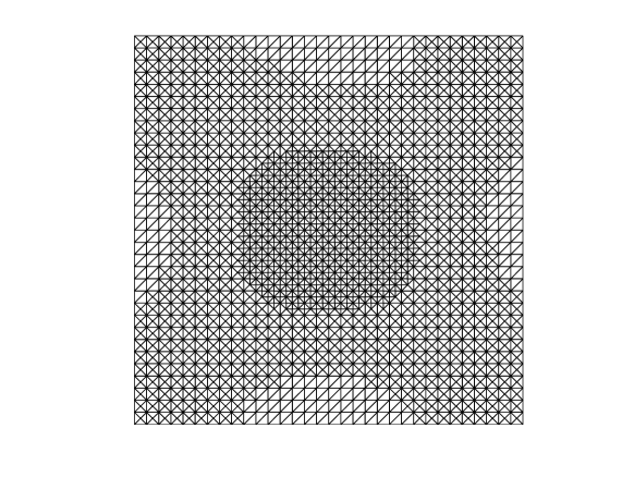
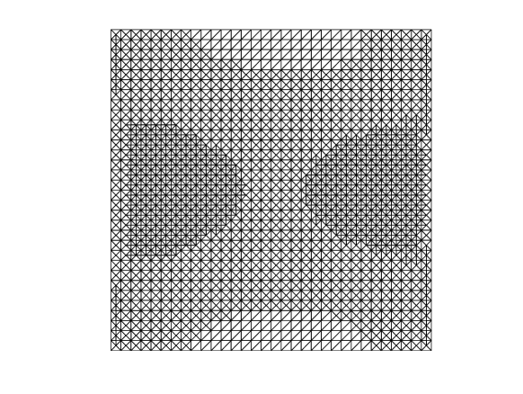
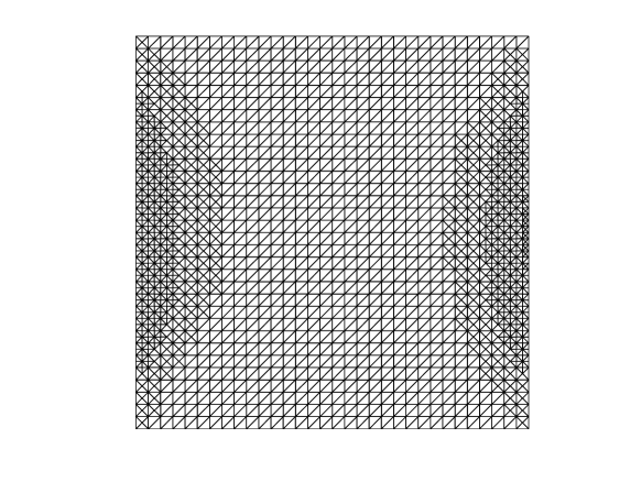
Figure 1: the adaptively refined meshes of 1st eigenvalue after 6th iteration when $\mathbf{b}=(1,0)^{T},\mathbf{b}=(3,0)^{T}$, and $\mathbf{b}=(10,0)^{T}$, respectively.

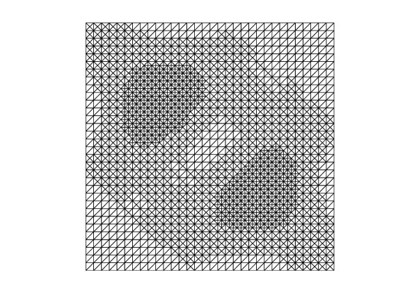
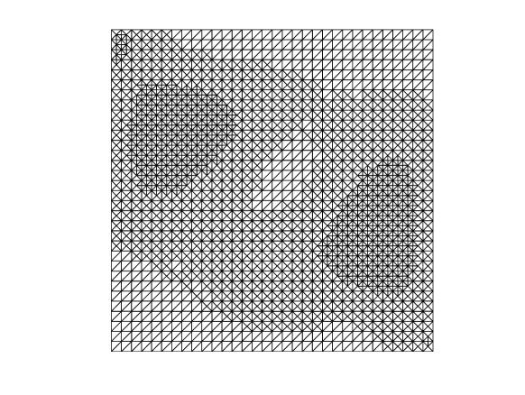
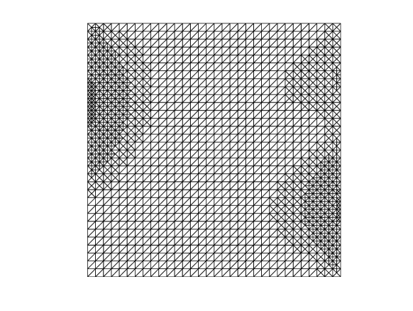
Figure 2: the adaptively refined meshes of 2nd eigenvalue after 6th iteration when $\mathbf{b}=(1,0)^{T},\mathbf{b}=(3,0)^{T}$, and $\mathbf{b}=(10,0)^{T}$, respectively.

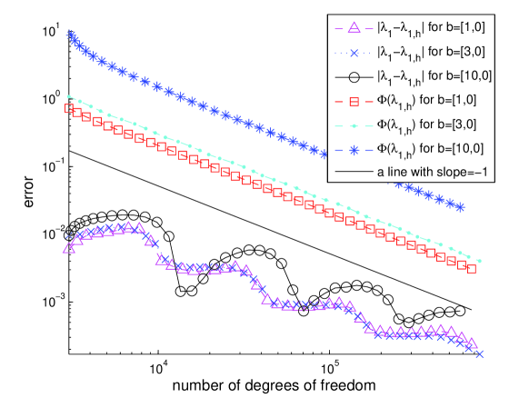
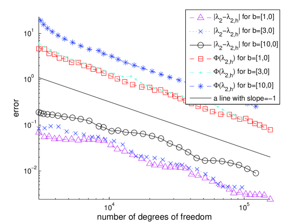
Figure 3: $\Omega=(0,1)^{2}$, the first eigenvalue and the second eigenvalue

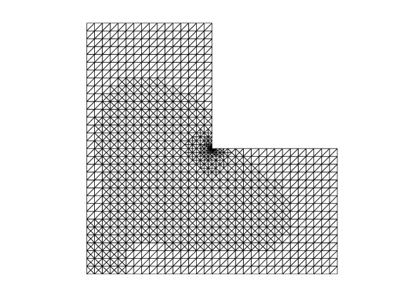
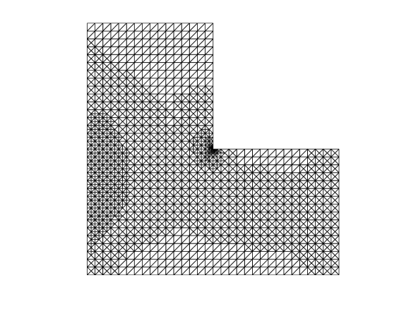
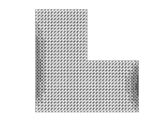
Figure 4: the adaptively refined meshes of 1st eigenvalue after 6th iteration when $\mathbf{b}=(1,0)^{T},\mathbf{b}=(3,0)^{T}$, and $\mathbf{b}=(10,0)^{T}$, respectively.

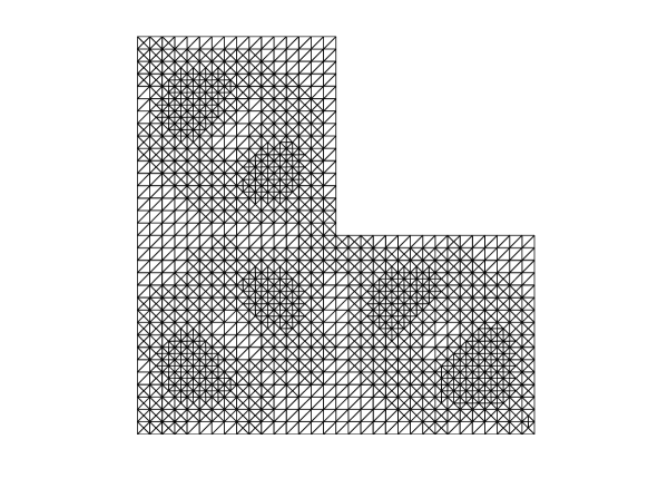
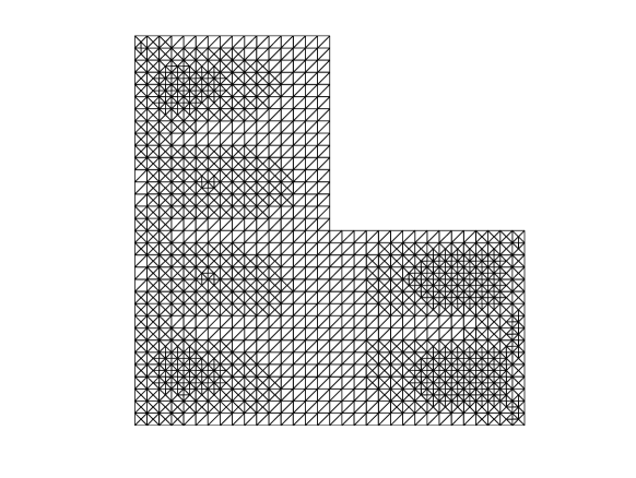
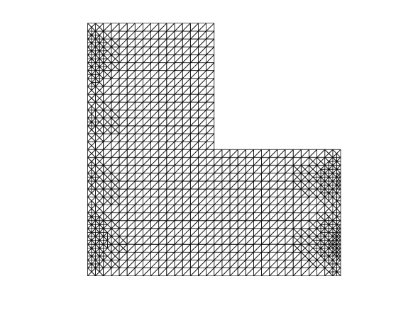
Figure 5: the adaptively refined meshes of 8th eigenvalue after 6th iteration when $\mathbf{b}=(1,0)^{T},\mathbf{b}=(3,0)^{T}$, and $\mathbf{b}=(10,0)^{T}$, respectively.

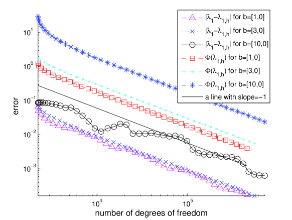
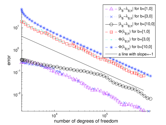
Figure 6: $\Omega=(0,2)^{2}\setminus[1,2]^{2}$, the first eigenvalue and the 8th eigenvalue

Table 1: The 1st and 2nd eigenvalues on $\Omega=(0,1)^{2}$ with $H=\frac{\sqrt{2}}{16}$.

$k$	$l$	$N_{k,l}(1)$	$\lambda_{k}(1)$	$N_{k,l}(3)$	$\lambda_{k}(3)$	$N_{k,l}(10)$	$\lambda_{k}(10)$
1	6	5846	19.977907	6113	21.976516	4171	44.755867
1	18	32624	19.986582	35943	21.987155	20781	44.743331
1	30	173175	19.988992	191642	21.989001	122039	44.740570
1	38	513308	19.989039	577955	21.989081	374065	44.739512
1	39	590647	19.989101	648352	21.989119	428658	44.739520
1	40	675033	19.989153	751651	21.989156	493913	44.739547
2	6	4757	49.54975734	5630	51.53186078	4174	74.18697239
2	18	17413	49.57934179	24916	51.58036988	24714	74.28997551
2	30	58202	49.59209659	96381	51.59363069	144114	74.33904514
2	38	130004	49.59500385	244514	51.59666467	436679	74.3446992
2	39	140739	49.59507564	266852	51.59682511	503989	74.34528594
2	40	155888	49.59561150	292042	51.59684387	578175	74.34579087

Table 2: The 1st and 8th eigenvalues on $\Omega=(0,2)^{2}\setminus[1,2]^{2}$ with $H=\frac{\sqrt{2}}{16}$.

$k$	$l$	$N_{k,l}(1)$	$\lambda_{k}(1)$	$N_{k,l}(3)$	$\lambda_{k}(3)$	$N_{k,l}(10)$	$\lambda_{k}(10)$
1	6	3278	9.868593	3876	11.863678	2686	34.725519
1	18	19789	9.885896	23820	11.885939	13141	34.655247
1	30	111849	9.889023	135412	11.889074	84307	34.648104
1	38	345699	9.889490	412412	11.889511	266844	34.641987
1	39	394793	9.889514	474643	11.889540	307313	34.641930
1	40	452105	9.889551	545221	11.889562	354041	34.641676
8	6	4103	49.336511	3671	51.372524	2902	74.010829
8	12	8791	49.476412	7272	51.428181	6220	74.123357
8	18	20394	49.536447	14189	51.510658	15446	74.193993
8	23	34979	49.564431	481420	51.595113	33382	74.229178
8	24	37940	49.567477	738241	51.596140	38817	74.231469
8	25	41981	49.573008	1433565	51.596812	45354	74.242124