A New Challenge to Solar Dynamo Models from Helioseismic Observations:
The Latitudinal Dependence of the Progression of the Solar Cycle

Abstract

The solar cycle onset at mid-latitudes, the slow down of the sunspot drift toward the equator, the tail-like attachment and the overlap of successive cycles at the time of activity minimum are delicate issues in $\alpha\Omega$ dynamo wave and flux transport dynamo models. Very different parameter values produce similar results, making it difficult to understand the origin of these solar cycle properties. We use GONG helioseismic data to investigate the progression of the solar cycle as observed in intermediate-degree global $p$-mode frequency shifts at different latitudes and subsurface layers, from the beginning of solar cycle 23 up to the maximum of the current solar cycle. We also analyze those for high-degree modes in each hemisphere obtained through the ring-diagram technique of local helioseismology. The analysis highlighted differences in the progression of the cycle below 15° compared to higher latitudes. While the cycle starts at mid-latitudes and then migrates equatorward/poleward, the sunspot eruptions of the old cycle are still ongoing below 15° latitude. This prolonged activity causes a delay in the cycle onset and an overlap of successive cycles, whose extension differs in the two hemispheres. Then the activity level rises faster reaching a maximum characterized by a single peak structure compared to the double peak at higher latitudes. Afterwards the descending phase shows up with a slower decay rate. The latitudinal properties of the solar cycle progression highlighted in this study provide useful constraints to discern among the multitude of solar dynamo models.

1 Introduction

The cyclic behavior of solar magnetic activity is ascribed to the dynamo process powered by the inductive action of the turbulent fluid in the Sun’s interior. A clear consensus has been reached on the $\Omega$ mechanism, which generates toroidal field by shearing a pre-existing poloidal field by differential rotation. Conversely it is still a matter of debate which $\alpha$ - effect regenerates poloidal fields from toroidal ones. There are two main competitive mechanisms: 1) the $\alpha$ turbulent effect, which regenerates poloidal field from toroidal flux tube by helical motion (Parker, 1955); 2) the Babcock - Leighton mechanism, which is based on the observed decay of tilted, bipolar active regions, which acts as poloidal field sources at the surface (Babcock, 1961; Leighton, 1964). While the $\alpha$ - turbulent $\Omega$ dynamo offered a plausible explanation for the sunspot drift toward equatorial latitudes by a dynamo wave, the Babcock - Leighton mechanism failed to reproduce the butterfly diagram. Therefore for several decades the $\alpha$-turbulent $\Omega$ dynamo has been favored over the Babcock - Leighton mechanism. As various observations have found a poleward surface meridional flow (Duvall, 1979; Komm et al., 1993; Hathaway, 1996), the inclusion of a poleward circulation along with an equatorward subsurface return flow, initiated the development of so called Flux Transport Dynamo (FTD) model. This new class of dynamo models revived the Babcock - Leighton mechanism, as its inclusion in FTD models has been successful in reproducing many global solar cycle features (Wang et al., 1991; Dikpati & Charbonneau, 1999; Nandy & Choudhuri, 2001). The resulting simulations showed that the butterfly diagram is produced by the equatorward subsurface return flow advecting the toroidal field toward the equator. They have also been developed $\alpha$-turbulent $\Omega$ FTD models operating in the tachocline (Dikpati & Gilman, 2001) and FTD simultaneously driven by an $\alpha$- turbulent effect located or in the tachocline or in the whole convection zone and a Babcock - Leighton type surface poloidal sources (Belucz & Dikpati, 2013; Passos et al., 2014). The key question is whether the Babcock - Leighton mechanism is an active component of the dynamo cycle, or a mere consequence of active region decay. How well the FTD and/or dynamo wave models reproduce the features observed in the butterfly diagram, might help solving the puzzle.

Fig. 1 shows the main features of the butterfly diagram: 1) the onset of cycle at mid-latitudes; 2) the sunspot drift toward the equator and its slow down represented by a change in the slope of the butterfly wing (Maunder, 1904; Li et al., 2001); 3) the tail-like attachment over the minimum phase more prominent when the activity is stronger, which might lead to the overlap of successive cycles; 4) the length of the overlap varies within 1 - 2 years. It characterizes only the minimum phase and it is confined at latitudes $\leq$ 15°  (Cliver, 2014). This feature is also seen in torsional oscillations shown in the bottom panels of Fig. 1 (Howe et al., 2009; Wilson et al., 1988). The sunspot drift rate toward the equator slows as the sunspot band approaches the equator, and halts at about 8$\arcdeg$ latitude (Hathaway et al., 2003). The end of the migration does not correspond to the end of the activity as it produces the tail-like attachment. When the new cycle at mid-latitudes starts before the end of the old cycle at low latitudes, it causes the overlap of successive cycles. FTD models driven only by Babcock - Leighton mechanism (Chatterjee et al., 2004) or along with the $\alpha$ -turbulent effect operating in the bulk of the convection zone, currently, have the best agreement with observations (Passos et al., 2014), as the length of the simulated overlap is short and it occurs only during the minimum at low latitudes. Conversely, thin shell dynamo wave models (Moss & Brooke, 2000; Bushby, 2006; Schüssler & Schmitt, 2004) or flux transport thin shell dynamo (Dikpati & Gilman, 2001), tend to produce dynamo waves with too short wavelength leading to excessive overlap between adjacent cycles as it involves a wider range of latitudes. Furthermore they also fail to reproduce the tail - like attachment over the minimum phase. Moreover the direction of the activity migration could also provide information on the nature of the $\alpha$ mechanism. Both formalisms make strong assumptions to initiate the sunspot cycle at mid-latitudes. The Babcock - Leighton FTD models assume that the deep equatorward meridional flow penetrates slightly below the convection zone to a greater depth than usually believed (Nandy & Choudhuri, 2002), to prevent the onset and occurrence of a sunspot cycle above 45$\arcdeg$ as well as any other kind of cyclic activity. The same result is achieved in $\alpha\Omega$ dynamo wave by inhibiting the $\alpha$ - turbulent effect at higher latitudes (Schüssler & Schmitt, 2004). Based on these assumptions in any type of FTD models the magnetic activity starts at higher latitudes and then propagates only equatorward, while in thin shell $\alpha\Omega$ dynamo wave the magnetic activity can propagate equatorward as well as poleward (Bushby, 2006). These two branches are also clearly seen in the torsional oscillation pattern (e.g. Howe et al., 2009). It results from the solar - like differential profile, which is characterized by a sign change in $\frac{\delta\Omega}{\delta r}$ at high - and low latitude tachocline (Ruediger & Brandenburg, 1995). This sign change, however has not yet been confirmed by helioseismic observations.

In this work we aim at characterizing the different phases of solar cycle at all latitudes and in the two hemispheres, as these properties can be used to constrain solar dynamo models. We use acoustic $p$-mode frequencies as a diagnostic tool to infer the progression of the 11 yr magnetic cycle. They are very well known to correlate strongly with solar magnetic activity (Elsworth et al., 1990; Libbrecht & Woodard, 1990; Howe et al., 1999; Jain et al., 2000; Simoniello et al., 2010) and unlike to many other solar activity proxies they probe magnetic changes induced by weak as well as strong toroidal fields at all latitudes. In order to simultaneously track solar magnetic activity in both hemispheres separately, we further use localized high-degree frequencies from the ring-diagram technique. The paper is organized as follows: in Sect. 2 we describe the data analysis for both intermediate and high-degree mode. The results are presented in Sect. 3 followed by the comparison with sunspot numbers in Sect. 4, and the findings are discussed in Sect. 5.

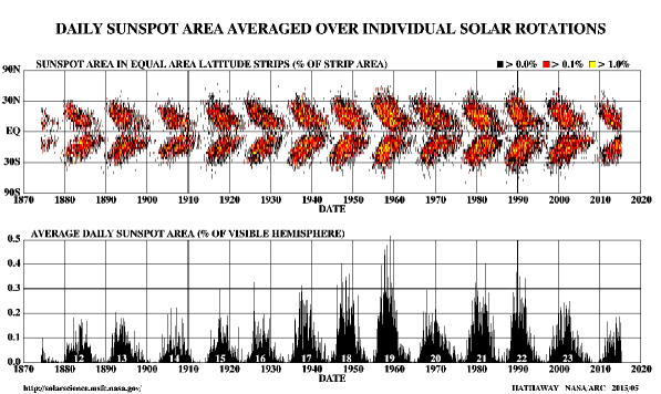
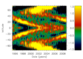
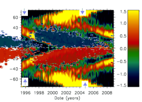
Figure 1: Top two panels show the butterfly diagram and the Sunspot area daily averaged (taken from www.msfc.nasa.gov). Bottom left panel show the torsional oscillations from Howe et al. (2009) and bottom right the same with the over plotted butterfly diagram provided by Solar Influences Data Center (SIDC) using sunspot numbers and rescaled to match the left panel. The plot extends outside the axes as the SIDC sunspot data have been over plotted since the descending phase of solar cycle 22, when GONG observations did not yet started (taken from https://landscheidt.wordpress.com/2009/02/25/latest-solar-differential-rotation-information/).The arrows identify the begin of the equatorward branch at around 40° .

2 Data Analysis

2.1 The GONG data

In this work we look for temporal variations in $p$-mode frequencies caused by changes in magnetic activity levels as function of latitude and subsurface layers. The mode frequencies analyzed here are obtained from the Global Oscillation Network Group (GONG) in two different degree ranges. The low-and intermediate-degree global mode frequencies are obtained for the individual ($n,\ell,m$) multiplets, $\nu_{n\ell m}$, where $n$ is the radial order and $m$ is the azimuthal order, running from $-\ell$ to $+\ell$. The mode frequencies for each multiplet were estimated from the $m-\nu$ power spectra constructed by the time series of 108 days. The data analyzed here consist of overlapping data sets, with a spacing of 36 days between consecutive time series, covering the period from June 1995 to July 2013 in the $\ell$ range of 20 $\leq\ell\leq$ 147 and frequency range 1500$\mu$Hz $\leq\nu\leq$ 3900$\mu$Hz.

The high-degree mode frequencies are obtained from the localized regions (15°$\times$ 15°) on the solar surface using the GONG ring-diagram pipeline (Corbard et al., 2003). The analysis covers a period from 2001 July to 2014 June in the degree range of 180 $\leq\ell\leq$ 1000. In the ring-diagram method, the localized regions on the solar surface are tracked with an average rotation rate at the solar surface for 1664 minutes. Each tracked area is apodized with a circular function and then a three-dimensional FFT is applied on both spatial and temporal direction to obtain a three-dimensional power spectrum. Finally, the corresponding power spectrum is fitted using a Lorentzian profile model to obtain acoustic mode parameters. The high-degree modes provide information about the outermost layer of the Sun’s interior.

2.2 Determination of the frequency shifts

We aim at characterizing the progression of solar cycle at different latitudes. The sunspot cycle starts at mid-latitudes ($\approx 30\arcdeg$ latitude), it reaches the maximum at $\approx$ 15° latitude and stops at around 8° latitude. Modes of low to intermediate degree $\ell$ are global, and sense the spherical geometry of the Sun. Therefore these are better described by spherical harmonics of the form $Y_{\ell,m}(\theta,\phi)=P_{\ell,m}(cos\theta)e^{im\phi}$, where P is the Legendre Polynomial, $\ell$ the spherical degree and $m$ the azimuthal order. The spherical harmonic degree $\ell$ is the number of nodes along a circle at an angle $\theta=arccos\frac{m}{\sqrt{(}\ell(\ell+1)}$ at the equator. The azimuthal order $m$ is the number of nodal lines crossing the equator. We, therefore, used the above ratio to select acoustic modes depending on their upper latitude range to which they are more sensitive. It may be noted that acoustic modes with same spherical degree $\ell$, but different azimuthal order $m$ increase their sensitivity to lower latitudes with increasing $m$. In fact the sectoral modes ($|{m}|$ = $\ell$) are more sensitive to the regions near the equator while the zonal modes ($m$ = 0) have higher sensitivity at higher latitudes (Hill et al., 1991). We carry on this selection in five latitude ranges between 0° $\leq\theta\leq$ 75° spaced by 15° . This allow us to split the cycle progression in latitude ranges. Since the acoustic waves travel throughout the interior and they reflect back from different layers depending on their frequencies, we further investigate the progression of the solar cycle based on their upper turning point ($u_{p}$). With increasing frequency $u_{p}$ approaches the surface (Basu et al., 2012). We divide frequency data sets in to three groups: (i) low-frequency range 1500 $\mu$Hz $\leq\nu\leq$ 2300 $\mu$Hz correspondes to 0.9944 R_⊙ $\leq u_{p}\leq$ 0.9987 R_⊙, (ii) medium-frequency range 2300 $\mu$Hz $\leq\nu\leq$ 3100 $\mu$Hz for 0.9987 R_⊙ $\leq u_{p}\leq$ 0.9998 R_⊙, and (iii) high-frequency range 3100 $\mu$Hz $\leq\nu\leq$ 3900 $\mu$Hz for 0.9998 R_⊙ $\leq u_{p}\leq$ 0.9999 R_⊙. As helioseismic observations have shown that the size of the frequency variation with the solar cycle increases as $u_{p}$ approaches the surface (Chaplin et al., 2001; Simoniello et al., 2013), we then calculated the frequency shifts in the low, medium and high frequency band, to investigate the solar cycle properties in different subsurface layers. Mode frequency shifts $\delta\nu_{n,\ell}(t)$ were defined as the differences between the frequencies observed at different times ($\nu_{n,\ell}(t)$) and the reference values of the corresponding modes ($\nu(ref)$):

$$\delta\nu_{n,\ell}(t)=\nu_{n,\ell}(t)-\nu_{n,\ell}(ref)$$ (1)

The $\nu_{n,\ell}(ref)$ was determined as the average frequency over the minimum between cycle 22 and 23. We took into account the period of observations from June 1995 up to May 1996. While we have included the end of activity cycle 22, we have been very careful not to include in $\nu_{n,\ell}(ref)$ the beginning of solar activity at higher latitudes, as it would have led significant differences in the size of $\nu_{n,\ell}(ref)$ at different latitudes making difficult any comparison and interpretation of the solar cycle properties. We then determine the weighted frequency difference in the low, medium and high frequency band for each selected latitude. The weights ($\frac{1}{\sigma^{2}}$), are the errors of the fitting procedure.

The high-degree mode frequency shifts were obtained by analyzing the frequencies obtained from from ring-diagram technique. These frequencies in localized regions are affected by the foreshortening as well as the gaps in observation, thus have been corrected by modeling these effects as a two-dimensional function of the distance from the disk center and a linear dependence of the duty cycle (Howe et al., 2004; Tripathy et al., 2013). The corrected frequencies are then used to compute frequency shifts which is computationally similar to those of global modes except for the choice of the reference frequency. For high-degree modes, the frequency difference of each mode is computed with respect to the average frequency of the same mode over the 189-dense pack tiles (covering $\pm$ 60°on the disk) corresponding to a magnetically quiet day (2008 May 11). In a similar manner frequency shifts for each hemisphere and at different latitude ranges were computed with an appropriate reference frequency as described in Tripathy et al. (2015) e.g. for northern hemisphere, the reference frequency was computed only over the northern hemisphere.

3 Results

3.1 Progression of solar cycle at different latitudes

Since numerous examples have clearly shown the strong correlation between frequency shifts and the magnetic activity indices over different time scales, we interpret frequency shifts as a measure of solar activity in rest of the paper.

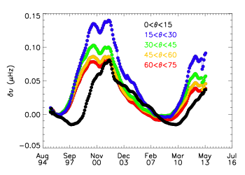
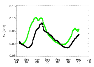
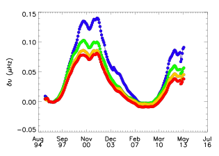
Figure 2: Top panel shows the variation of $p$-mode frequency shifts with time at five different latitudinal bands. Bottom row: left panel highlights the differences in the evolution of magnetic activity as measured by the frequency shifts during the descending phase between 0°$\leq\theta\leq$ 15° (black) and 30°$\leq\theta\leq$ 45° (green) while right panel shows the similarities in four latitude bands.

Top panel of Figure 2 shows the variation of frequency shifts over solar cycle 23 and the ascending phase of solar cycle 24 at five latitude bands in the frequency range of 1500 $\mu$Hz $\leq\nu\leq$ 3900 $\mu$Hz. All curves have been smoothed with a boxcar of 1 year and the estimated uncertainties are of the order 10${}^{-3}\mu$Hz. It is clearly seen that the progression of activity cycle is different at different latitudes. In particular, the variation of the magnetic activity below 15° differs from the one at higher latitudes; it rises faster, the maximum is characterized by a single peak structure and an excess of activity changes the evolutionary path of the descending phase around 2003 December. This difference is better highlighted in the bottom left panel of Figure 2, which compares the activity at 0° $\leq\theta\leq$ 15° with 30° $\leq\theta\leq$ 45°. At 0° $\leq\theta\leq$ 15°, the declining phase lasted longer compared to higher latitudes delaying the time of the minimum and the onset of solar cycle 24 for about a year, which led to an overlap of cycle 23 with cycle 24. Similar longer delay in the onset of solar cycle 23 caused an overlap between cycle 22 and 23. Furthermore over both minimum phases, the activity level reached its deepest value at latitudes between 0°$\leq\theta\leq$ 15°. The bottom right panel highlights the similarity in the progression of solar activity at all latitudes above 15°. Here, the activity level at both minimum phases at all latitude bands is of comparable size. It rises with slightly different growth rates and reaches the maximum characterized by the typical double peak structure, which has been interpreted as a manifestation of the Quasi-Biennial Periodicity (QBP; Fletcher et al., 2010; Jain et al., 2011; Simoniello et al., 2012, 2013). Soon after the second maximum, the descending phase continued with comparable decay times, although around 2003 December the progression at latitudes between 15°$\leq\theta\leq$ 30° slightly changed.

To summarize similarities and differences in the properties of the progression of solar cycle at different latitudes and in the low, medium and high frequency range, Table 1 lists (i) the epochs of minimum and maximum of solar cycle in each latitudinal band; these have been defined as the timing corresponding to the lowest/highest value in the frequency shift at different latitudes, (ii) the rising and decay time, (iii) the full cycle length. The solar cycle progression shows common features in the three bands: starts within the latitude range 30° $\leq\theta\leq$ 45° and followed by other latitudes. Between 0° $\leq\theta\leq$ 15° latitude the onset of the new cycle is always delayed, but this time lag disappears at the time of the maximum, as it occurs at the same epoch at all latitudes in each frequency range (Max(2) in Table 1). This result further confirms that the rise in activity below 15° latitude is faster compared to all other latitudes (Rise time (2) in Table 1). The descending phase, instead, lasted longer below 15° latitude compared to higher ones, leading to a slow down of the progression of magnetic activity, which ended in the overlap of successive cycles (Decay time in Table 1). This peculiar behavior ended up in a stronger asymmetry between the rise and decay time at latitudes below 15° compared to higher ones. Even though the descending phase lasted longer at latitudes $\leq$ 15° , the fastest rising phase made cycle lengths of comparable size at all latitudes in all frequency bands (Length in Table 1).

Table 1: The solar cycle onset, peak amplitude, rise and decay time, and the full cycle length in the low, medium and high frequency range.

Low Frequency Range
Lat	Cycle 23			Cycle 24	Rise (1)	Rise (2)	Decay	Length
Degree	Min	Max (1)	Max (2)	Min	Months	Months	Max-Min	Months
0$\leq\theta\leq$15	02/1998		03/2002	03/2010		49	96	145
15$\leq\theta\leq$30	03/1996	06/2000	03/2002	11/2007	51	72	68	140
30$\leq\theta\leq$45	01/1996	05/2000	03/2002	07/2007	52	74	64	138
45$\leq\theta\leq$60	08/1996	04/2000	03/2002	07/2007	44	67	64	131
60$\leq\theta\leq$75	09/1996	04/2000	03/2002	08/2007	43	66	65	132
Medium Frequency Range
0$\leq\theta\leq$15	11/1997		04/2002	01/2010		53	93	146
15$\leq\theta\leq$30	09/1996	07/2000	04/2002	04/2009	46	67	84	151
30$\leq\theta\leq$45	06/1996	06/2000	03/2002	05/2008	48	69	74	143
45$\leq\theta\leq$60	07/1996	06/2000	03/2002	11/2008	47	68	80	148
60$\leq\theta\leq$75	08/1996	05/2000	03/2002	12/2008	45	67	81	148
High Frequency Range
0$\leq\theta\leq$15	12/1997		04/2002	01/2010		52	93	145
15$\leq\theta\leq$30	09/1996	06/2000	03/2002	03/2009	45	66	84	150
30$\leq\theta\leq$45	09/1996	06/2000	03/2002	10/2008	45	66	79	145
45$\leq\theta\leq$60	10/1996	06/2000	03/2002	11/2008	44	65	80	145
60$\leq\theta\leq$75	11/1996	06/2000	03/2002	12/2008	43	64	81	145

3.2 Sensitivity of the progression of solar cycle to the subsurface layers

To further study whether such behavior persists in the solar subsurface layers, each panel of Fig. 3 shows the progression of solar cycle in a selected frequency band and at all latitudes. As we can see the properties of the two different modes of the solar cycle as described above do not change.

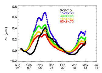
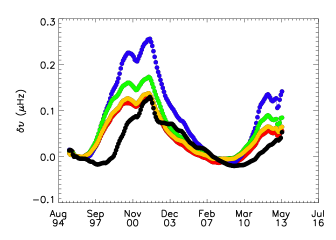
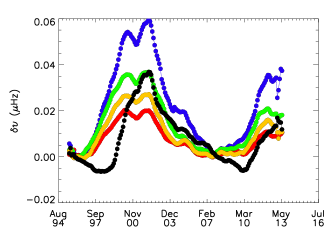
Figure 3: Solar cycle changes in $p$-mode frequency shifts at five different latitudinal bands in three different frequency ranges: (top) 3100 $\mu$Hz $\leq\nu\leq$ 3900 $\mu$Hz, (middle) 2300 $\mu$Hz $\leq\nu\leq$ 3100 $\mu$Hz, and (bottom) 1500 $\mu$Hz $\leq\nu\leq$ 2300 $\mu$Hz. Note that the scales on y-axis in all three plots are different.

To better compare the behavior and strength of activity in the three subsurface layers, each panel of Fig. 4 compares the activity at the same latitude but in the three frequency ranges. As expected the activity is stronger in the nearest subsurface layers compared to deeper ones.

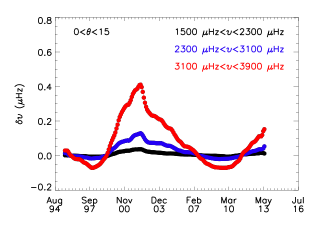
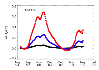
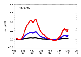
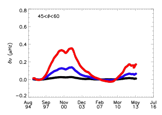
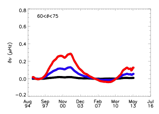
Figure 4: Each panel shows the progression of solar cycle 23 and 24 at specific latitude but in three frequency bands corresponding to different subsurface layers. From top to bottom the progression of solar cycle with increasing latitude.

3.3 Progression of solar cycle in the Northern and Southern hemispheres

The top two panels of Fig. 5 show the progression of solar cycle in the Northern and Southern hemispheres as determined by the analysis of the high degree modes in two different latitudinal bands. While in the Northern hemisphere the activity is almost comparable at the two selected latitudes, the activity in the Southern is higher at the maximum between 15° $\leq\theta\leq$ 30° latitude, to then reach comparable strengths sometime after December 2003. After September 2006 the activity between 0° $\leq\theta\leq$ 15° and 15° $\leq\theta\leq$ 30° latitudes followed different patterns. In fact, while below 15° we observe a prolonged minimum until June 2009 with a consequent delay in the onset of solar cycle either hemisphere (shown by black), above 15° latitude the rising phase already started sometime after September 2006 (shown by red).

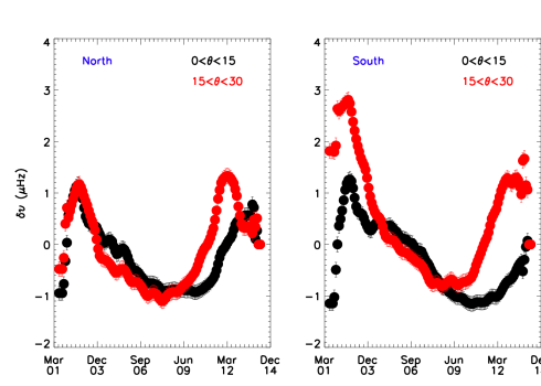
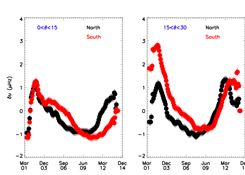
Figure 5: Top two panels: Progression of the solar cycle as seen in high-degree mode frequency shifts in northern (left) and southern (right) hemispheres in two different latitude ranges. Bottom two panels: Comparison of the progression of solar cycle between northern and southern hemispheres in the same latitude range; 0° $\leq\theta\leq$ 15° (left), and 15° $\leq\theta\leq$ 30°  (right)

When we compare the strength of activity at the same latitude but for different hemispheres (bottom two panels of Fig. 5), we find that throughout the descending phase the Southern hemisphere (shown by red) has been more active compared to the Northern one (shown by black). In particular we note an enhancement in the activity, which changes the evolutionary path of the descending phase at latitudes between 0° $\leq\theta\leq$ 15° (bottom left panel). This deviation is stronger in the Southern hemisphere. Interestingly where the excess of magnetic activity is more pronounced, the descending phase is consequently slightly more prolonged, leading to a longer overlap of successive cycles. Table 2 lists the time of the minimum in both Southern and Northern hemisphere and at two latitudes. In the Southern hemisphere the overlap of successive cycles lasted slightly more than in the Northern hemisphere. Comparing the timing of the minimum between both hemispheres, we note that the two hemispheres are in delay with respect to each other by approximately one year.

Table 2: The minimum epochs in the two hemispheres as seen from high-degree modes

Latitude	Cycle 23		Min-Min
Degree	Min South	Min North	Diff
0$\leq\theta\leq$15	10/2010	09/2009	13
15$\leq\theta\leq$30	06/2008	09/2007	9

4 Correlation with Sunspot

4.1 STARA data

In order to compare the variation of oscillation frequencies with known proxies of the solar activity, we use sunspot numbers calculated from the Sunspot Tracking And Recognition Algorithm (STARA; Watson et al. (2011)). In STARA sunspot catalogue, the sunspot count does not include a factor for grouped sunspots and so the number is far lower than other sources. The sunspot numbers are calculated using the MDI images for the period from June 1996 to October 2010. Although, there are some gaps in data due to the SOHO vacation in 1998-99, the advantage of using this catalogue over others is the availability of the location of sunspots on solar disk which is important in this analysis. The sunspot numbers beyond 2010 are also available but have been calculated using the HMI images which have different spatial resolution and no scaling has been performed yet.

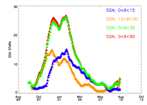
Figure 6: The STARA Sunspot Number at different latitudes as indicated in the figure.

Fig. 6 shows the sunspot numbers as measured by STARA; the gaps are due to unavailability of data. The sunspot numbers are the averages over the same period as the time series of the oscillation frequencies. We further grouped them in three latitude bands. In the analysis of global modes, the selection of a particular latitude range does not confine modes’ sensitivity to the selected range. Instead it senses all latitudes between northern and southern hemispheres up to the highest selected latitude. Thus frequency shifts in 15° $\leq\theta\leq$ 30° range, which covers modes in latitudes $\pm$ 30°  are compared with the sunspot data between $\pm$ 30° latitude. There were no sunspots observed in 15° $\leq\theta\leq$ 30° latitude ranges before 1996 August, while some were visible in 0°  $\leq\theta\leq$ 15° bands since the beginning of the available data, i.e., 1996 June.

Over the minimum phase between cycle 22 and 23, we notice that magnetic cycle started when the activity of the old cycle was still ongoing below 15° latitude. We also note that the maximum is characterized by a double peak structure for latitudes between 0°$\leq\theta\leq$ 30°, while by a single peak structure between 0°  $\leq\theta\leq$ 15°, as already found in our helioseismic analysis of intermediate degree modes. Furthermore soon after December 2003 an excess of sunspots at latitudes of 0° $\leq\theta\leq$ 15°changed the natural evolution of the activity during the descending phase.

4.2 Frequency shifts and STARA Sunspots

We aim at comparing STARA Sunspot number with helioseismic observations to highlight similarities and differences in the progression of the cycle between the two activity proxies. They are sensitive to different magnetic field structures. Sunspot are the result of the strong toroidal fields located at around equatorial latitudes, while acoustic waves sounds the whole Sun at all latitudes. Therefore they are sensitive to strong and weak toroidal fields. To compare the behavior of the two activity proxies, we treated the STARA SSN data as we did for the mode frequency. We determined the SSN reference values (SSN_ref) between December 1996 - March 1997, the common period of quiet activity phase where SSN at all latitudes are around two. Then we calculate the deviation $\delta SSN$ as the differences between the observed sunspot at different epochs (SSN) and the SSN_ref. Finally $\delta SSN$ and $\delta\nu$ have been divided for the sum of the shifts/sunspots throughout the observational time, which gave us $\delta SSN_{rel}$ and $\delta\nu_{rel}$. Fig. 7 compares the behavior of solar magnetic activity from STARA data with frequency shifts determined in the high frequency band at each selected latitude, as the high frequency range sounds the closest layer to the solar surface. It is worth reminding that, as the reference values for $\delta SSN$ and $\delta\nu$ have been calculated over different periods of activity and the length of observations span different time lengths, we cannot directly compare the size of $\delta SSN_{rel}$ and $\delta\nu_{rel}$, however the overall trend can be compared. Nevertheless we find that both activity proxies are characterized by a single peak structure at latitudes below 15°  while above it by a double peak structure. This further confirms that the single peak structure is a signature of the solar magnetic activity at 0° $\leq\theta\leq$ 15° latitude ranges. Although the origin of $p$-mode frequency shifts is still a matter of debate, magnetic fields in Sunspots can widen or shrink the acoustic cavity (Schunker & Cally, 2006; Simoniello et al., 2010), shifting the mode frequency towards lower/higher values. We might argue that during the descending phase, soon after December 2003, an excess of emergence of Sunspots produced the observed enhancement in the size of the shift predominantly in the Southern hemisphere and at latitudes below 15° .

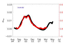
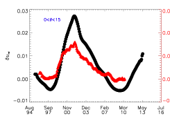
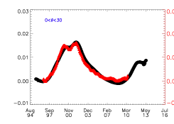
Figure 7: Comparison between $\delta SSN_{rel}$ (red) and $\delta\nu_{rel}$ (black) at three different latitudes. Top panel show the temporal variation of these two quantities averaged over disk, while bottom row shows the variation in two latitudinal bands: 0° $\leq\theta\leq$ 15° (left), and 0° $\leq\theta\leq$ 30° (right).

5 Discussion

Solar cycle changes in p-mode frequencies are unique tools to investigate similarities and differences in the progression of solar cycle at different latitudes and subsurface layers. In addition, high degree modes calculated from local helioseismology techniques open a window on the solar hemispheric activity. In this work, therefore, we use intermediate and high degree acoustic modes to obtain a detailed description of the Sun s global and hemispheric magnetism.

The latitudinal and frequency dependence of solar cycle changes in p-mode frequency shifts from intermediate degree modes is a different representation of what is seen in the butterfly diagram and latitudinal inversions of the helioseismic modes (Howe et al., 2002). However, this approach highlighted new important details, which could be used to constrain the sources of the $\alpha$ mechanism.

The overall results have pointed out latitudinal differences in the solar cycle progression below and above 15° in both hemispheres. The cycle onset below 15° is delayed compared to higher latitudes, causing an overlap of successive cycle at the time of the minimum phase. To this regard the analysis of high degree modes identified and quantified, for the first time, differences in the length of the overlap of successive cycles in the two hemispheres. Furthermore in both hemispheres our findings confine the overlap at latitudes below 15° . Soon after the minimum, the activity level below 15° progresses with the fastest rise time and it reaches the maximum characterized by a single peak. At higher latitudes instead the ascending phase is characterized by a slower rise time and it ends up in a maximum characterized by a double peak structure. Interestingly the single peak below 15° coincides with the second and highest peak at higher latitudes. The dynamo mechanism seems to synchronize the epoch of the maximum at all latitudes. During the descending phase we found latitudinal differences in the decay time, as it is slower below 15° compared to higher latitudes.

How these observed properties can help us in understanding the role of the BL poloidal field sources with respect to the $\alpha$ turbulent one? For example, our findings have provided evidences that the overlap occur at latitudes below 15° . This confinement is better reproduced in FTD models including the Babcock - Leighton mechanism. Therefore we might envisage that to some extension the Babcock-Leighton mechanism might play a role in the solar dynamo (Cameron & Schüssler, 2015), but to draw any conclusion all the solar cycle features need to be reproduced within this formalism. In fact the meridional flow speed sets the cycle period, the rise and decay time within BL flux transport dynamo. Within the $\alpha$ turbulent $\omega$ dynamo the cycle period depends (among others) on the $\alpha$ turbulent effect itself (Parker, 1955). It would be then rather interesting to see how our findings will impose further constraints on the latitudinal dependence of the meridional flow speed and $\alpha$ turbulent effect. How well the resulting simulations will fit with observations, will be a valuable test to discern among the multitude of dynamo models and it will shed some light on the principle driving solar dynamo.

References

- Babcock (1961) Babcock, H. W. 1961, ApJ, 133, 572
- Basu et al. (2012) Basu, S., Broomhall, A. M., Elsworth, Y., & Chaplin, W. J. 2012, ApJ, 758, 43B
- Belucz & Dikpati (2013) Belucz, B., & Dikpati, M. 2013, ApJ, 779, 4
- Bushby (2006) Bushby, P. J. 2006, MNRAS, 371, 772
- Cameron & Schüssler (2015) Cameron, R., & Schüssler, M. 2015, Science, 347, 1333
- Chaplin et al. (2001) Chaplin, W. J., Appourchaux, T. Elsworth, Y. P., & Isaak, G. R. 2001, MNRAS, 324, 910
- Chatterjee et al. (2004) Chatterjee, P., Nandy, D., & Choudhuri, A. R. 2004, A&A, 427, 1019
- Cliver (2014) Cliver, E. W. 2014, Space Sci. Rev., 186, 169
- Corbard et al. (2003) Corbard, T., Toner, C., Hill, F., Hanna, K. D., Haber, D. A., Hindman, B. W., & Bogart, R. S. 2003, in ESA Special Publication, Vol. 517, GONG+ 2002. Local and Global Helioseismology: the Present and Future, ed. H. Sawaya-Lacoste, 255–258
- Dikpati & Charbonneau (1999) Dikpati, M., & Charbonneau, P. 1999, ApJ, 518, 508
- Dikpati & Gilman (2001) Dikpati, M., & Gilman, P. A. 2001, ApJ, 559, 428
- Duvall (1979) Duvall, Jr., T. L. 1979, Sol. Phys., 63, 3
- Elsworth et al. (1990) Elsworth, Y., Howe, R., Isaak, G. R., McLeod, C. P., & New, R. 1990, Nature, 345, 322
- Fletcher et al. (2010) Fletcher, S., Broomhall, A. M., Salabert, D., et al. 2010, ApJ, 718L, 19
- Hathaway (1996) Hathaway, D. H. 1996, ApJ, 460, 1027
- Hathaway et al. (2003) Hathaway, D. H., Nandy, D., Wilson, R. M., & Reichmann, E. J. 2003, ApJ, 589, 665
- Hill et al. (1991) Hill, F., Deubner, F., & Issak, G. 1991, Oscillation Observations, ed. A. Cox, W. Livingston, & M. Matthews, 329
- Howe et al. (2009) Howe, R., Christensen-Dalsgaard, J., Hill, F., et al. 2009, ApJ, 701, 87
- Howe et al. (1999) Howe, R., Komm, R., & Hill, F. 1999, ApJ, 524, 1084
- Howe et al. (2002) —. 2002, ApJ, 580, 1172
- Howe et al. (2004) Howe, R., Komm, R. W., Hill, F., Haber, D. A., & Hindman, B. W. 2004, ApJ, 608, 562
- Jain et al. (2000) Jain, K., Tripathy, S. C., & Bhatnagar, A. 2000, ApJ, 542, 521
- Jain et al. (2011) Jain, K., Tripathy, S. C., & Hill, F. 2011, ApJ, 739, 6
- Komm et al. (1993) Komm, R. W., Howard, R. F., & Harvey, J. W. 1993, Sol. Phys., 147, 207
- Leighton (1964) Leighton, R. B. 1964, ApJ, 140, 1547
- Li et al. (2001) Li, K. J., Yun, H. S., & Gu, X. M. 2001, Astronomical Journal, 122, 2115
- Libbrecht & Woodard (1990) Libbrecht, K. G., & Woodard, M. F. 1990, Nature, 345, 779
- MacGregor & Charbonneau (1997) MacGregor, K. B., & Charbonneau, P. 1997, ApJ, 486, 484
- Maunder (1904) Maunder, E. W. 1904, Popular Astronomy, 12, 616
- Moss & Brooke (2000) Moss, D., & Brooke, J. 2000, MNRAS, 315, 521
- Nandy & Choudhuri (2001) Nandy, D., & Choudhuri, A. R. 2001, ApJ, 551, 576
- Nandy & Choudhuri (2002) —. 2002, Science, 296, 1671
- Parker (1955) Parker, E. N. 1955, ApJ, 121, 491
- Parker (1993) —. 1993, ApJ, 408, 707
- Passos et al. (2014) Passos, D., Nandy, D., Hazra, S., & Lopes, I. 2014, AA, 563, A18
- Ruediger & Brandenburg (1995) Ruediger, G., & Brandenburg, A. 1995, A&A, 296, 557
- Schunker & Cally (2006) Schunker, H., & Cally, P. S. 2006, MNRAS, 372, 551
- Schüssler & Schmitt (2004) Schüssler, M., & Schmitt, D. 2004, AA, 421, 349
- Simoniello et al. (2010) Simoniello, R., Finsterle, W., García, R. A., et al. 2010, AA, 516, 30
- Simoniello et al. (2012) Simoniello, R., Finsterle, W., Salabert, D., et al. 2012, AA, 539, 135
- Simoniello et al. (2013) Simoniello, R., Jain, K., Tripathy, S. C., Turck-Chièze, S., Baldner, C., Finsterle, W., Hill, F., & Roth, M. 2013, ApJ, 765, 100
- Tripathy et al. (2013) Tripathy, S. C., Jain, K., & Hill, F. 2013, Sol. Phys., 282, 1
- Tripathy et al. (2015) —. 2015, ApJ, 812, 20
- Wang et al. (1991) Wang, Y.-M., Sheeley, Jr., N. R., & Nash, A. G. 1991, ApJ, 383, 431
- Watson et al. (2011) Watson, F. T., Fletcher, L., & Marshall, S. 2011, AA, 533, A14
- Wilson et al. (1988) Wilson, P. R., Altrocki, R. C., Harvey, K. L., Martin, S. F., & Snodgrass, H. B. 1988, Nature, 333, 748