Detection of a hot molecular core in the Large Magellanic Cloud with ALMA

Abstract

We report the first detection of a hot molecular core outside our Galaxy based on radio observations with ALMA toward a high-mass young stellar object (YSO) in a nearby low metallicity galaxy, the Large Magellanic Cloud (LMC). Molecular emission lines of CO, C¹⁷O, HCO⁺, H¹³CO⁺, H₂CO, NO, SiO, H₂CS, ³³SO, ³²SO₂, ³⁴SO₂, and ³³SO₂ are detected from a compact region ($\sim$0.1 pc) associated with a high-mass YSO, ST11. The temperature of molecular gas is estimated to be higher than 100 K based on rotation diagram analysis of SO₂ and ³⁴SO₂ lines. The compact source size, warm gas temperature, high density, and rich molecular lines around a high-mass protostar suggest that ST11 is associated with a hot molecular core. We find that the molecular abundances of the LMC hot core are significantly different from those of Galactic hot cores. The abundances of CH₃OH, H₂CO, and HNCO are remarkably lower compared with Galactic hot cores by at least 1–3 orders of magnitude. We suggest that these abundances are characterized by the deficiency of molecules whose formation requires the hydrogenation of CO on grain surfaces. In contrast, NO shows a high abundance in ST11 despite the notably low abundance of nitrogen in the LMC. A multitude of SO₂ and its isotopologue line detections in ST11 imply that SO₂ can be a key molecular tracer of hot core chemistry in metal-poor environments. Furthermore, we find molecular outflows around the hot core, which is the second detection of an extragalactic protostellar outflow. In this paper, we discuss physical and chemical characteristics of a hot molecular core in the low metallicity environment.

1 Introduction

Because cosmic metallicity is increasing in time with the evolution of our universe, interstellar chemistry in low metallicity environments is crucial to understand chemical processes in the past universe. For this purpose, observations of chemically-rich objects in nearby low metallicity galaxies and comparative studies with Galactic counterparts play an important role.

Hot molecular cores are one of the early stages of high-mass star formation and they play a key role in the formation and evolution of complex molecules in space. In terms of physical properties, hot cores are defined as having small source size ($\leq$0.1 pc), high density ($\geq$10⁶ cm^-3), and warm gas/dust temperature ($\geq$100 K) (e.g., Kurtz et al., 2000; van der Tak, 2004). Chemistry of hot cores is characterized by sublimation of ice mantles, which accumulated in the course of star formation. In cold molecular clouds and prestellar cores, gaseous molecules and atoms are frozen onto dust grains and hydrogenated. As the core is heated by star-formation activities, reaction among heavy species become active on grain surfaces to form larger molecules. In addition, sublimated molecules, such as CH₃OH and NH₃, are subject to further gas-phase reactions (e.g., Garrod & Herbst, 2006; Garrod et al., 2008; Herbst & van Dishoeck, 2009). As a result, hot cores show a wealth of molecular spectral lines in infrared and radio wavelengths. Thus detailed studies of chemical properties of hot cores are crucial to understand complex chemical processes triggered by star formation.

The Large Magellanic Cloud (LMC) is an excellent target to study interstellar and circumstellar chemistry in different metallicity environments owing to its proximity (49.97 $\pm$ 1.11 kpc, Pietrzyński et al., 2013) and low metallicity (about one third of the solar neighborhood, Westerlund, 1990). The low dust content in the galaxy results in harsh radiation environment, and thus photoprocessing of interstellar medium should be more effective in the LMC than in our Galaxy (Israel et al., 1986). Furthermore, according to gamma-ray observations, the cosmic-ray density in the LMC is estimated to be lower than the Galactic typical values by a factor of four (Abdo et al., 2010). It is therefore highly anticipated that these environmental differences should affect chemical processes, and hot cores in the LMC should provide us key information to understand chemistry, particularly those of complex molecules, in low metallicity environments. However, so far, observations of hot cores have been limited to Galactic sources due to lack of spatial resolution and sensitivity of radio telescopes.

Most of radio studies on chemical compositions of molecular gas in the LMC have been performed with single-dish telescopes. Early studies by the SEST 15 m telescope conducted multiline observations toward H II regions in the LMC and detected molecular species as large as CH₃OH, C₃H₂ and SO₂ (Johansson et al., 1994; Chin et al., 1997; Heikkilä et al., 1999; Wang et al., 2009). Submillimeter observations of relatively dense molecular gas in star-forming regions in the LMC are also reported (Paron et al., 2014, 2016). Nishimura et al. (2016) recently conducted deep and unbiased spectral line surveys in the 3 mm window toward a number of molecular clouds in the LMC using the Mopra telescope. They reported the low abundances of nitrogen-bearing molecules, the deficiency of CH₃OH, and the high abundance of C₂H in the LMC compared with Galactic molecular clouds.

Characteristic interstellar chemistry in the LMC is also suggested from previous infrared observations of ices around embedded young stellar objects (YSOs) in the LMC. Shimonishi et al. (2008, 2010) reported that the CO₂/H₂O ice ratio of high-mass YSOs in the LMC is systematically higher than those of Galactic high-mass YSOs based on infrared observations with the AKARI satellite. Recently, Shimonishi et al. (2016) reported that the CH₃OH ice around high-mass YSOs in the LMC is less abundant compared with Galactic counterparts based on infrared observations with the Very Large Telescope. The authors suggest that warm ice chemistry (grain surface reactions at a relatively high dust temperature) is responsible for the observed characteristics of ice chemical compositions in the LMC. Furthermore, detailed studies of the 15.2 $\mu$m CO₂ ice band toward LMC high-mass YSOs with Spitzer suggest a higher degree of thermal processing of ices in the LMC than in our Galaxy (Oliveira et al., 2009; Seale et al., 2011). Since gas-grain chemistry is believed to play an important role in hot cores, the characteristic ice chemistry in the LMC would imply diverse hot core chemistry in extragalactic environments according to their metallicities.

High-spatial resolution interferometry observations toward star-forming regions in the LMC have been reported with the Australia Telescope Compact Array (e.g., Wong et al., 2006; Ott et al., 2008; Seale et al., 2012; Anderson et al., 2014) and recently with the Atacama Large Millimeter/submillimeter Array (ALMA) (e.g., Indebetouw et al., 2013; Fukui et al., 2015). These observations resolve star-forming regions in the LMC down to parsec- or sub-parsec-scale and investigate physical properties of dense molecular gas. However, chemical properties of warm and dense molecular gas associated with a single high-mass YSO in the LMC still remain to be investigated.

In this paper, we report the detection of a hot molecular core in the LMC based on submillimeter interferometric observations with ALMA. In $\S$ 2 we describe the details of observations and data reduction conducted in this work. Obtained images and spectra of molecular line emission and continuum are presented in $\S$ 3. Analysis of spectral line data and derivation of physical quantities of molecular gas and dust are described in $\S$ 4. Physical and chemical properties of the observed source are discussed in $\S$ 5. Finally, conclusions of this paper are summarized in $\S$ 6.

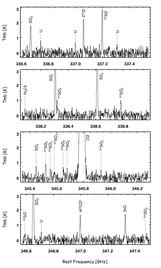
Figure 1: ALMA band 7 spectra of ST11 extracted from the central region with a radius of 0.5$\arcsec$. Detected emission lines are labeled. Tentative detections are indicated by “?” and unidentified lines are by “U”. The adopted source velocity is 250.5 km/s.

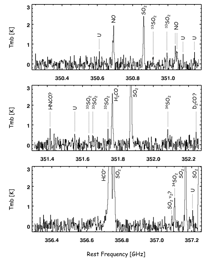
Figure 2: Continued

2 Observations and data reduction

2.1 Target

The target of the present observations is a high-mass YSO, 2MASS J05264658-6848469 or ST11 (hereafter ST11), located in the LMC. The source is spectroscopically identified to be a high-mass YSO in previous infrared studies (Seale et al., 2009; Shimonishi et al., 2010). Detailed YSO properties of ST11 are revisited in this work and discussed in $\S$ 4.5.

2.2 Observations

Observations were carried out with ALMA between November 2013 and February 2014 as a part of the Cycle 1 high priority program 2012.1.01108.S (PI T. Shimonishi). The telescopes were pointed to RA = 05^h26^m46$\fs$63 and Dec = -68^∘48$\arcmin$47$\farcs$10 (J2000), which is a position of ST11 measured by infrared data (Shimonishi et al., 2010). The compact configurations C32-3 and partially C32-2 were used for our observations. The target object was observed in Band 7 with seven spectral bands covering 336.60–337.55, 338.05-339.00, 345.35–346.30, 346.55–347.50, 350.25–351.20, 351.30–352.25, and 356.30–357.25 GHz in the rest-frame frequency. The observed lines and the integration times are presented in Table 1. The primary beam has a full-width at half-maximum (FWHM) of 18–19$\arcsec$ at these frequencies, which corresponds to the field-of-view (FoV) of imaging data. The maximum recoverable angular scale is about 7$\arcsec$. The velocity resolution of the original data is 0.4 km/s for the spectral bands and 26 km/s for the continuum band.

2.3 Data reduction

Raw interferometric data is processed using the Common Astronomy Software Applications (CASA) package. The calibration is done by CASA 4.1.0 and imaging as well as spectral extraction are done by CASA 4.3.0. The flux calibrator is J0519-454 and the phase calibrators are J0601-7036 and J0635-7516. The synthesized beam size in the 338 GHz region is approximately 0.5$\arcsec$ $\times$ 0.5$\arcsec$, which corresponds to 0.12 pc at the assumed distance to the LMC (49.97 kpc, Pietrzyński et al., 2013). The primary beam correction is done by the impbcor task in CASA, but the correction have little effect on the extracted spectra since the target source is located at the center of FoV and very compact.

The spectra as well as continuum flux are extracted from the circular region with a diameter of 0.5$\arcsec$ centered at RA = 05^h26^m46$\fs$60 and Dec = -68^∘48$\arcmin$47$\farcs$03 (J2000). This region corresponds to the peak position of the 359 GHz (840 $\mu$m) continuum emission of ST11 measured in this study, and the diameter corresponds to the beam size. The continuum emission is subtracted from the spectral data using the uvcontsub task in CASA. Several channels are concatenated during the clean process to increase S/N and the channel spacing of the reduced data is 1.5 km/s (1.73 MHz) except for CO(3–2). For the CO(3–2) line, the spectral region is not binned since the line is sufficiently strong, and the channel spacing is 0.4 km/s (0.46 MHz).

3 Results

3.1 Observed spectra

Figures 1–2 show the spectra extracted from the 0.5$\arcsec$ diameter region centered at ST11. In the figures the sky frequency is converted to the rest frequency using the LSR velocity of 250.5 km/s, which is the typical radial velocity of molecular lines detected toward the source. Spectral lines are identified with the aid of the Cologne Database for Molecular Spectroscopy (CDMS, Müller et al., 2001, 2005) and the molecular database of the Jet Propulsion Laboratory (JPL, Pickett et al., 1998). Molecular emission lines due to CO, C¹⁷O, HCO⁺, H¹³CO⁺, H₂CO, NO, SiO, H₂CS, ³³SO, ³²SO₂, ³⁴SO₂, and ³³SO₂ are detected from a compact region associated with ST11. A number of high excitation lines ($E_{u}$ $>$100 K) are detected for SO₂ and its isotopologues. The emission lines of the above molecules in the 345 GHz band are for the first time detected toward the LMC source except for CO and HCO⁺. Emission lines of CH₃OH, HNCO, CS, HC₃N, and complex organic molecules are not detected. Unidentified lines are labeled in the figures, but some of them may be spurious signals.

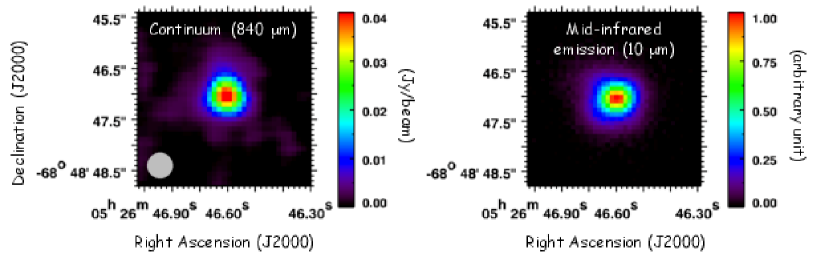
Figure 3: Flux distribution of the ALMA 840 $\mu$m continuum data tracing cold dust (left) and the Gemini/T-ReCS mid-infrared 10 $\mu$m image tracing warm dust (right).

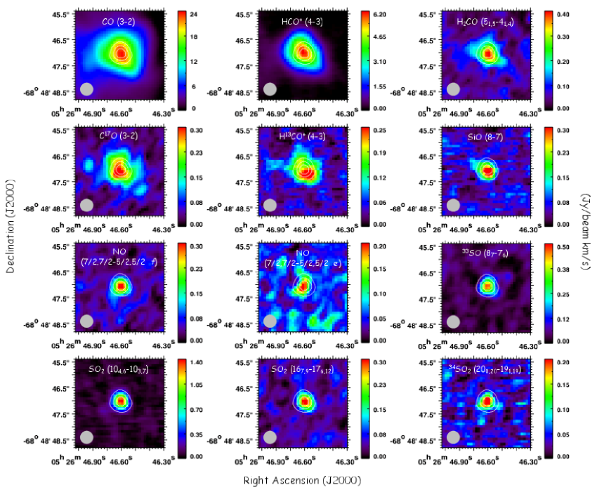
Figure 4: Integrated intensity distributions of CO, C¹⁷O, HCO⁺, H¹³CO⁺, H₂CO, SiO, NO, ³³SO, SO₂, and ³⁴SO₂ lines. Contours represent the distribution of the 840 $\mu$m continuum, and the contour levels are 25 $\%$, 50 $\%$ and 75 $\%$ of the peak flux. The synthesized beam size (0.5$\arcsec$, 0.12 pc at the LMC) is shown by the gray filled circle in each panel.

3.2 Synthesized images

Figures 3–4 show synthesized images of continuum and molecular emission lines observed toward ST11. For SO₂ and ³⁴SO₂, we only show representative lines because distributions of emission are similar in different transitions. The lines of SO₂ ($\nu$₂ = 1), ³³SO₂, and H₂CS are not included in the figure because they are too weak to visualize the brightness distribution. The images are constructed by integrating each spectrum in the velocity range where the emission line is seen, typically between 240 km/s and 260 km/s. For CO, the spectrum is integrated between 230 km/s and 285 km/s because the line is very broad.

A high spatial resolution mid-infrared image of ST11 is also shown in Figure 3. The image is obtained by T-ReCS at the Gemini South telescope (Program ID: S10B-120, PI: T. Shimonishi) and a broad-band filter in the N-band (7.70–12.97 $\mu$m, centered at 10.36 $\mu$m) is used for the observation. The ALMA 840 $\mu$m continuum traces distribution of cold dust, while the mid-infrared image traces warm dust.

The source is compact in general and peak positions of each emission line coincide with the region of dust continuum emission. We estimate a source size (Gaussian FWHM, $\theta$) for continuum and relatively strong emission lines by a two-dimensional Gaussian fit. The estimated $\theta$ in the 840 $\mu$m continuum image is about 0.6$\arcsec$, which is close to the beam size. The mid-infrared emission shows $\theta$ = 0.5$\arcsec$, which is as compact as the 840 $\mu$m continuum. The molecular lines of NO, SiO, ³³SO, SO₂, and ³⁴SO₂ typically have $\theta$ $\sim$0.5$\arcsec$, which is indistinguishable from the beam size. Since the distribution is as compact as the beam size, these emissions are considered to be a point source with the present spatial resolution. The H¹³CO⁺ and H₂CO lines are slightly extended compared with the above lines and have $\theta$ $\sim$0.8$\arcsec$. The lines of CO, C¹⁷O and HCO⁺ are more extended and $\theta$ is 1.1$\arcsec$–1.4$\arcsec$. Because the source size is sufficiently smaller than the maximum recoverable angular scale of $\sim$7$\arcsec$, the emission from ST11 is almost recovered by the present interferometric observations.

4 Analysis

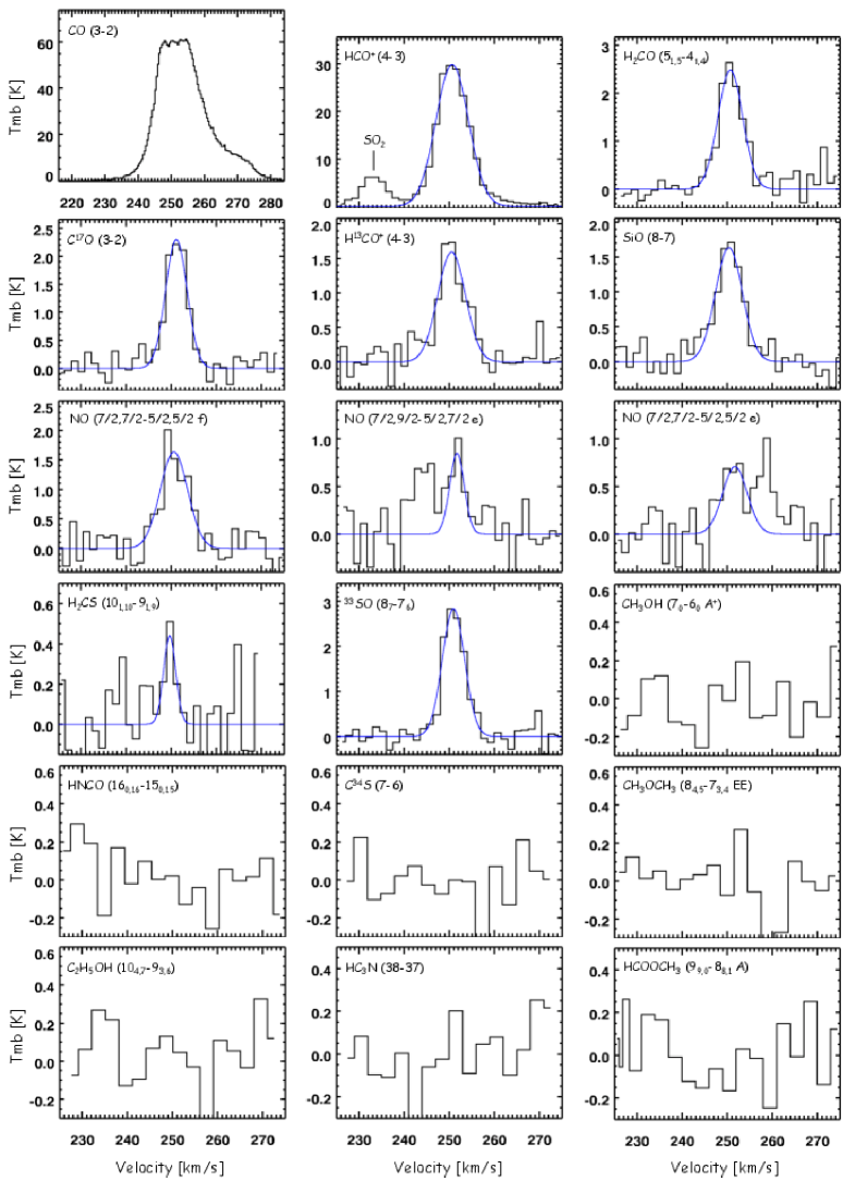
Figure 5: Spectra of CO, C¹⁷O, HCO⁺, H¹³CO⁺, H₂CO, SiO, NO, H₂CS, and ³³SO emission lines extracted from the 0.5$\arcsec$ diameter region centered at ST11. The blue lines represent Gaussian profiles fitted to the observed spectra. The spectral regions of important non-detection lines including CH₃OH, HNCO, C³⁴S, CH₃OCH₃, C₂H₅OH, HC₃N, and HCOOCH₃ are also shown.

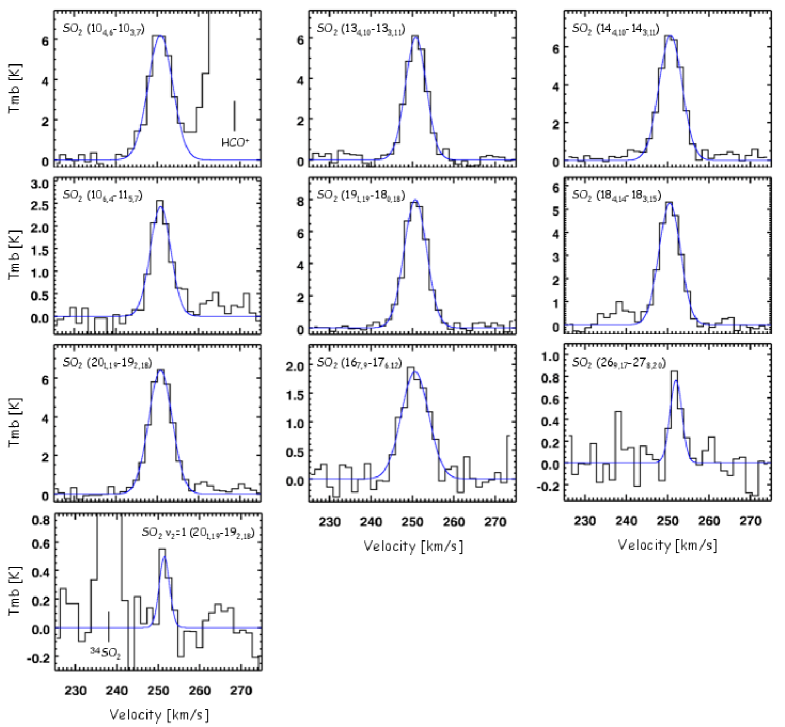
Figure 6: Spectra of SO₂ emission lines extracted from the 0.5$\arcsec$ diameter region centered at ST11. The blue lines represent a Gaussian profile fitted to the observed spectra. The spectra are sorted in ascending order of the upper state energy (The emission line with the lowest upper state energy is shown in the upper left panel and that with the highest energy is in the lower right panel). The bottom panel is for the SO₂ ($\nu$₂ = 1) line.

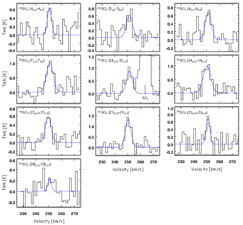
Figure 7: Spectra of ³⁴SO₂ emission lines observed toward ST11 as in Figure 6. The spectra are sorted in ascending order of the upper state energy from the upper left to the lower right.

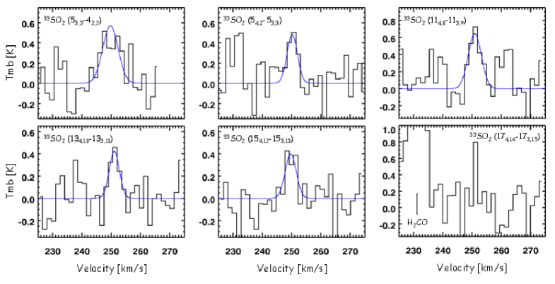
Figure 8: Spectra of ³³SO₂ emission lines observed toward ST11 as in Figure 6. The spectra are sorted in ascending order of the upper state energy from the upper left to the lower right. The 17_4,14–17_3,15 line is a tentative detection.

4.1 Spectral fitting

The line parameters are measured by fitting a single Gaussian profile to the observed lines. For the NO lines at 351.0435 GHz and 351.0515 GHz, we fit a double Gaussian because they are partially blended. In some cases we subtract a local baseline, which is estimated from adjacent line-free regions to correct for weak baseline ripples. For the SO₂(10_4,6–10_3,7) line, we subtracted the HCO⁺(4–3) line upon fitting since they are partly blended. In general, good fits are obtained with Gaussian profiles except for the CO(3–2) line, which deviates from a Gaussian. We estimate a peak main-beam brightness temperature, a FWHM, a LSR velocity, and an integrated intensity for each line on the basis of the fitting. For CO, instead, we estimate the peak brightness temperature and the FWHM by visual inspection, and the integrated intensity is estimated by integrating the spectrum in the velocity range between 230 km/s and 285 km/s. The spectra and the results of the gaussian fitting are shown Figures 5–8. The figures also show the spectral regions of several important non-detection lines. The measured line parameters are summarized in Table 1.

Multiple hyperfine components sometime exist within fitted profile according to the spectroscopic catalogues (CDMS or JPL), but these are not resolved due to the low spectral resolution of the present spectra. When the blended lines have comparable upper state energies, we split the measured flux according to the their $S\mu^{2}$ values and the upper state degeneracy (see $\S$ 4.2 for definition of $S$ and $\mu$). Using this method, we estimate the line parameters of the strongest hyperfine line, which is used in the subsequent analysis of column densities and rotational temperatures.

4.2 Rotation diagram analysis for SO₂, ³⁴SO₂ and ³³SO₂

Since we detect multiple emission lines with different excitation energies for SO₂, ³⁴SO₂ and ³³SO₂, we perform the rotation diagram analysis assuming an optically thin condition and an local thermodynamic equilibrium (LTE). A column density of molecules in the upper energy level, $N_{u}^{thin}$, is derived by the following equation for optically thin lines (e.g., Sutton et al., 1995; Goldsmith & Langer, 1999),

$$\frac{N_{u}^{thin}}{g_{u}}=\frac{3k\int T_{mb}dV}{8\pi^{3}\nu S\mu^{2}},$$ (1)

where $g_{u}$ is the degeneracy of the upper level, $k$ is the Boltzmann constant, $\int T_{mb}dV$ is the integrated intensity as estimated from the observations, $\nu$ is the transition frequency, $S$ is the line strength, and $\mu$ is the dipole moment. Under the LTE condition, the total column density, $N_{total}$, is given by

$$\frac{N_{u}^{thin}}{g_{u}}=\frac{N_{total}}{Q(T_{rot})}e^{-E_{u}/kT_{rot}},$$ (2)

where $Q(T_{rot})$ is the partition function, $T_{rot}$ is the rotational temperature, and $E_{u}$ is the upper state energy. This equation is rearranged as follows.

$$\log\left(\frac{N_{u}^{thin}}{g_{u}}\right)=-\left(\frac{\log e}{T_{rot}}\right)\left(\frac{E_{u}}{k}\right)+\log\left(\frac{N_{total}}{Q(T_{rot})}\right)$$ (3)

When $N_{u}^{thin}/g_{u}$ is plotted against $E_{u}/k$ and data points are fitted by a straight-line, the slope and the intercept correspond to $T_{rot}$ and $N_{total}$, respectively. Thus we can simultaneously determine the rotational temperature and the total column density. All the spectroscopic parameters required in the above analysis are extracted from the CDMS or the JPL database. For the partition function, we interpolate the data given in the databases and estimate the appropriate $Q(T_{rot})$ at the derived rotational temperature.

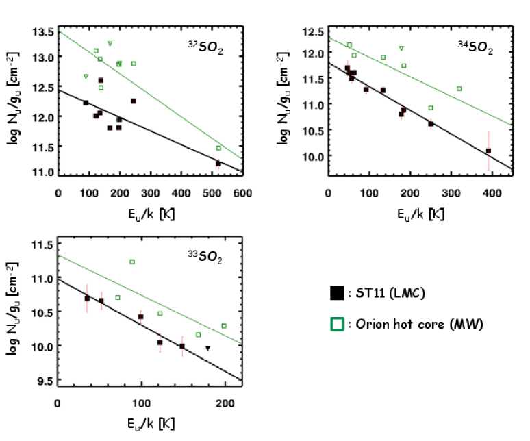
Figure 9: Rotation diagram analysis of ³²SO₂ (upper left), ³⁴SO₂ (upper right), and ³³SO₂ (lower left) for ST11. The filled squares (black) are for ST11 and the open squares (green) are for the Orion hot core. The downward triangles represent upper limits. The straight-lines fitted to the ST11 and the Orion data points are shown by the black and green solid lines, respectively. The derived rotational temperatures are shown in Table 4.3.

The constructed rotation diagrams for SO₂, ³⁴SO₂ and ³³SO₂ are shown in Figure 9 and the derived temperatures and column densities are summarized in Table 2. Uncertainties in the table are of 2 $\sigma$ level and do not include systematic errors due to spectroscopic parameters extracted from the CDMS and JPL databases.

For a comparison purpose, we also perform the rotation diagram analysis for the Orion hot core using the lines with the similar spectroscopic properties with those used in the analysis of ST11. The Orion data is obtained with the 20$\arcsec$ beam size ($\sim$0.04 pc at the Orion region) and adopted from Schilke et al. (1997). The rotational temperatures of the Orion hot core derived here are somewhat lower than temperatures derived in Schilke et al. (1997) using complete spectral line survey data in 325–360 GHz. This is because high excitation lines used in our comparative analysis are fewer than those used in Schilke et al. (1997) to allow for a fair comparison. The above results are shown in Figure 9 and Table 4.3 together with the results of ST11. The table also shows rotational temperatures of SO₂ and ³⁴SO₂ measured for W3 (H₂O) and G34.3+0.15, which are obtained from the literature (Helmich & van Dishoeck, 1997; MacDonald et al., 1996).

4.3 Column densities of other molecules

Column densities of other molecular species than SO₂ and its isotopologues are derived by solving Eq. 2 for $N_{total}$ under assumption of the LTE and optically thin condition. We here assume that the observed molecular species are located in the same region as SO₂ and its isotopologues, and thus have the similar rotational temperatures; $T_{rot}$ is assumed to be 100 K, which is roughly the average rotational temperature of SO₂, ³⁴SO₂ and ³³SO₂.

The similar spatial distributions of emission and the similar radial velocities of SO₂ and other molecules support the validity of this assumption, but more rigorous excitation analysis with further spectral data is absolutely necessary in the future.

NO shows multiple transitions with the same upper state energy in the 350–351 GHz region. We estimate the column density for each transition, and the average value is adopted as the final NO column density. The scatter of column densities estimated from different lines is less than 20 $\%$.

We also estimate upper limits on column densities of important non-detection lines such as CH₃OH, HNCO, C³⁴S and some complex molecules (see $\S\ref{sec_X_mol}$ for details of individual lines). Upper limits on peak brightness temperatures are measured using the observed spectra after appropriate channel binning, and then we assume the FWHM of 6 km/s to estimate the upper limits on integrated intensities. This FWHM is consistent with the typical velocity width of other molecular lines except for CO and HCO⁺.

The derived column densities and upper limits (2 $\sigma$ level) are summarized in Table 2.

Table 1: Line Parameters

Molecule	Transition	$Eu/k$	Frequency	$T_{mb}$	$\Delta$$V$	$\int T_{mb}dV$	$V_{LSR}$	RMS	$I_{\mathrm{time}}$	Note
		(K)	(GHz)	(K)	(km/s)	(K km/s)	(km/s)	(K)	(s)
CO	3–2	33	345.7960	$\sim$65	$\sim$16	$\sim$1150	$\sim$252	0.42	‡	1
C17O	3–2	32	337.0611	2.30 $\pm$ 0.08	5.6	13.77 $\pm$ 0.98	251.1	0.21	†
HCO+	4–3	43	356.7342	29.87 $\pm$ 0.08	8.5	270.86 $\pm$ 1.73	250.6	0.21	‡
H13CO+	4–3	42	346.9983	1.59 $\pm$ 0.06	7.3	12.34 $\pm$ 1.07	250.5	0.20	‡
NO	7/2,9/2–5/2,7/2 $f$	36	350.6895	1.63 $\pm$ 0.06	7.2	12.53 $\pm$ 0.97	250.6	0.19	†	2
	7/2,7/2–5/2,5/2 $f$	36	350.6908
	7/2,5/2–5/2,3/2 $f$	36	350.6948
NO	7/2,9/2–5/2,7/2 $e$	36	351.0435	0.85 $\pm$ 0.08	3.8	3.44 $\pm$ 0.69	251.7	0.19	†
NO	7/2,7/2–5/2,5/2 $e$	36	351.0515	0.71 $\pm$ 0.07	6.5	4.86 $\pm$ 0.97	251.7	0.19	†	3
	7/2,5/2–5/2,3/2 $e$	36	351.0517
H2CO	51,5–41,4	62	351.7686	2.48 $\pm$ 0.07	6.5	17.10 $\pm$ 1.02	250.7	0.20	†
CH3OH	70–60 A+	65	338.4087	$<$0.30	$\cdots$	$<$1.9	$\cdots$	0.15	†
HNCO	160,16–150,15	143	351.6333	$<$0.28	$\cdots$	$<$1.8	$\cdots$	0.14	†
SiO	8–7	75	347.3306	1.64 $\pm$ 0.06	7.1	12.32 $\pm$ 1.05	250.4	0.20	‡
C34S	7–6	65	337.3965	$<$0.30	$\cdots$	$<$1.9	$\cdots$	0.15	†
H2CS	101,10–91,9	102	338.0832	0.44 $\pm$ 0.07	3.2	1.49 $\pm$ 0.50	249.6	0.21	†
CH3OCH3	84,5–73,4 AE	55	356.5753	$<$0.30	$\cdots$	$<$1.9	$\cdots$	0.15	‡	3
	84,5–73,4 EE	55	356.5760
C2H5OH	104,7–93,6	66	357.0674	$<$0.30	$\cdots$	$<$1.9	$\cdots$	0.15	‡
33SO	87–76	81	337.1986	2.84 $\pm$ 0.07	5.8	17.63 $\pm$ 1.00	250.9	0.21	†	4
HC3N	38–37	323	345.6090	$<$0.27	$\cdots$	$<$1.7	$\cdots$	0.13	‡
HCOOCH3	99,0–88,1 A	80	345.7187	$<$0.27	$\cdots$	$<$1.7	$\cdots$	0.13	‡	3
	99,1–88,0 A	80	345.7187
SO2	167,9–176,12	245	336.6696	1.87 $\pm$ 0.07	7.8	15.50 $\pm$ 1.19	250.6	0.21	†
SO2	184,14–183,15	197	338.3060	5.25 $\pm$ 0.07	6.2	34.54 $\pm$ 1.08	250.5	0.21	†
SO2	201,19–192,18	199	338.6118	6.39 $\pm$ 0.07	6.7	45.67 $\pm$ 1.02	250.8	0.21	†
SO2	269,17–278,20	521	345.4490	0.76 $\pm$ 0.07	3.4	2.76 $\pm$ 0.53	252.0	0.19	‡
SO2	191,19–180,18	168	346.6522	7.99 $\pm$ 0.07	6.5	54.93 $\pm$ 1.00	250.7	0.20	‡
SO2	106,4–115,7	139	350.8628	2.43 $\pm$ 0.06	5.8	15.10 $\pm$ 0.85	250.8	0.19	†
SO2	144,10–143,11	136	351.8739	6.62 $\pm$ 0.07	6.6	46.24 $\pm$ 1.01	250.7	0.20	†
SO2	104,6–103,7	90	356.7552	6.19 $\pm$ 0.07	7.0	46.21 $\pm$ 1.18	250.8	0.21	‡	5
SO2	134,10–133,11	123	357.1654	6.03 $\pm$ 0.07	6.0	38.25 $\pm$ 0.95	250.8	0.21	‡
SO2 $\nu$2=1	53,3–42,2	781	357.0872	0.50 $\pm$ 0.07	3.0	1.56 $\pm$ 0.49	251.5	0.21	‡
33SO2	53,3–42,2	35	346.5901	0.57 $\pm$ 0.06	6.2	3.76 $\pm$ 1.62	249.7	0.20	‡	6
33SO2	134,10–133,11	122	350.7881	0.42 $\pm$ 0.05	4.1	1.83 $\pm$ 0.55	251.1	0.19	†	7
33SO2	154,12–153,13	149	350.9146	0.40 $\pm$ 0.06	4.5	1.89 $\pm$ 0.61	249.7	0.19	†	7
33SO2	114,8–113,9	99	350.9951	0.64 $\pm$ 0.05	5.3	3.64 $\pm$ 0.75	250.9	0.19	†	7
33SO2	54,2–53,3	52	351.6351	0.48 $\pm$ 0.06	4.2	2.16 $\pm$ 0.59	250.2	0.20	†	7
33SO2	174,14–173,15	179	351.7449	$<$0.80	$\cdots$	$<$2.4	$\cdots$	0.20	†	7
34SO2	132,12–121,11	92	338.3204	0.87 $\pm$ 0.06	5.6	5.14 $\pm$ 0.83	251.4	0.21	†
34SO2	144,10–143,11	134	338.7857	0.98 $\pm$ 0.06	6.9	7.26 $\pm$ 1.07	250.2	0.21	†
34SO2	74,4–73,5	64	345.5197	1.01 $\pm$ 0.07	6.1	6.59 $\pm$ 0.93	250.9	0.19	‡
34SO2	64,2–63,3	57	345.5531	0.67 $\pm$ 0.06	5.6	4.03 $\pm$ 0.77	251.2	0.19	‡
34SO2	54,2–53,3	52	345.6513	0.61 $\pm$ 0.05	5.6	3.66 $\pm$ 0.84	251.4	0.19	‡
34SO2	44,0–43,1	47	345.6788	0.64 $\pm$ 0.08	3.7	2.49 $\pm$ 0.72	250.6	0.19	‡
34SO2	174,14–173,15	179	345.9293	0.59 $\pm$ 0.05	5.0	3.16 $\pm$ 0.67	249.7	0.19	‡
34SO2	282,26–281,27	391	347.4831	0.23 $\pm$ 0.06	3.3	0.78 $\pm$ 0.54	250.7	0.20	‡
34SO2	214,18–213,19	250	352.0829	0.68 $\pm$ 0.07	3.6	2.62 $\pm$ 0.57	251.0	0.20	†
34SO2	200,20–191,19	185	357.1022	1.32 $\pm$ 0.07	5.2	7.27 $\pm$ 0.80	250.4	0.21	‡

Note. — Uncertainties and upper limits are of 2 $\sigma$ level and do not include systematic errors due to baseline subtraction and adopted spectroscopic constants. ^aTotal on-source integration time, where ${\dagger}$ represents 575 seconds and ${\ddagger}$ 1452 seconds. (1) Saturated. (2) Blended with three hyperfine components. (3) Blend with two hyperfine components. (4) Blend with four hyperfine components. (5) Partly blended with HCO⁺(4–3), which is subtracted when fitting this SO₂ line. (6) Blend with seven hyperfine components. (7) Blend with ten hyperfine components.

Table 2: Estimated column densities

Molecule	$T$rot	$N$(X)
	(K)	(cm-2)
SO2	190	8.4 $\pm$ 0.3 $\times$ 1015
34SO2	95	6.2 $\pm$ 0.9 $\times$ 1014
33SO2	64	2.1 $\pm$ 0.7 $\times$ 1014
H2	–	4.5 $\times$ 1023
CO	100	$\sim$8 $\times$ 1017
C17O	100	1.2 $\pm$ 0.09 $\times$ 1016
HCO+	100	1.4 $\pm$ 0.01 $\times$ 1014
H13CO+	100	6.9 $\pm$ 0.6 $\times$ 1012
H2CO	100	1.0 $\pm$ 0.1 $\times$ 1014
CH3OH	100	$<$3.5 $\times$ 1014
NO	100	9.1 $\pm$ 2.5 $\times$ 1015
HNCO	100	$<$4.3 $\times$ 1013
HC3N	100	$<$1.8 $\times$ 1013
SiO	100	1.5 $\pm$ 0.1 $\times$ 1013
C34S	100	$<$1.0 $\times$ 1013
H2CS	100	2.8 $\pm$ 0.9 $\times$ 1013
33SO	100	2.7 $\pm$ 0.6 $\times$ 1014
CH3OCH3	100	$<$1.3 $\times$ 1015
HCOOCH3	100	$<$7.1 $\times$ 1015
C2H5OH	100	$<$2.2 $\times$ 1015

Note. — Uncertainties and upper limits are of 2 $\sigma$ level and do not include systematic errors due to adopted spectroscopic constants.

^∗Derived based on the rotation diagram analysis (see $\S$ 4.2 for details).

Table 3: Comparison of rotational temperatures

	$T$rot [K]
Molecule	ST11	Orion-KL	W3 (H2O)	G34.3+0.15
SO2	190 $\pm$ 5	124 (121 $\pm$ 4)	184	108, 284
34SO2	95 $\pm$ 7	138 (114 $\pm$ 6)	179	131
33SO2	64 $\pm$ 14	104 (73 $\pm$ 5)	$\cdots$	$\cdots$

Note. — Uncertainties are of 2 $\sigma$ level.

^∗Numbers in parentheses in the Orion data are derived in this work (see $\S$ 4.2 for details). ^∗∗Two temperature components.

References. — ^aThis work; ^bSchilke et al. (1997); ^cHelmich & van Dishoeck (1997); ^dMacDonald et al. (1996)

4.4 Column density of H₂ and total gas mass

A column density of molecular hydrogen, which usually dominate the total mass of embedded sources, is estimated using the dust continuum emission data obtained in our observations. The flux density of dust continuum, $F_{\nu}$, at the optically thin frequency, $\nu$, is expressed as

$$F_{\nu}=\Omega\tau_{\nu}B_{\nu}(T_{d}),$$ (4)

where $\Omega$ is a beam solid angle, $\tau_{\nu}$ is an optical depth, $B_{\nu}(T_{d})$ is the Planck function and $T_{d}$ is a dust temperature (Whittet, 1992). The optical depth is expressed as

$$\tau_{\nu}=\rho_{d}\kappa_{\nu}L,$$ (5)

where $\rho_{d}$ is a mass density of dust, $\kappa_{\nu}$ is a mass absorption coefficient, and $L$ is a path length. We use the mass absorption coefficient of dust grains coated by thin ice mantles as presented in Ossenkopf & Henning (1994). Using the dust-to-gas mass ratio, $Z$, the mass density of dust is expressed as

$$\rho_{d}=Z\mu\rho_{\mathrm{H}}=Z\mu N_{\mathrm{H}}m_{\mathrm{H}}/L,$$ (6)

where $\mu$ is a mean atomic mass per hydrogen, $\rho_{H}$ is a mass density of hydrogen, $N_{H}$ is a column density of hydrogen, and $m_{H}$ is a hydrogen mass. We here assume $\mu$ to be 1.41 according to Cox (2000). We assume that the dust-to-gas mass ratio in the LMC is lower than the typical Galactic value of 0.008 by a factor of three according to Bernard et al. (2008), and we use $Z$ = 0.0027 in this work. By combining Equations 4–6, and assuming that all the hydrogen is in the form of H₂ ($N_{H_{2}}$ = $N_{H}/2$), the column density of molecular hydrogen is derived by the following equation:

$$N_{\mathrm{H_{2}}}=\frac{F_{\nu}/\Omega}{2\kappa_{\nu}B_{\nu}(T_{d})Z\mu m_{\mathrm{H}}}.$$ (7)

We measure the flux density per beam solid angle, $F_{\nu}/\Omega$, using the 840 $\mu$m dust continuum image of ST11 shown in Figure 3. With the aperture size of 0.5$\arcsec$ in diameter, the $F_{\nu}/\Omega$ is measured to be 0.34 Jy/beam. For dust temperature, we assume $T_{d}$ = 40 K, which is a typical dust temperature of high-mass YSOs in the LMC estimated based on far-infrared observations (van Loon et al., 2010). The assumed dust temperature is consistent with the far-infrared SED peak of ST11 (see $\S$ 4.5 for description of the SED). Using Equation 7 and the above parameters, we estimate $N_{H_{2}}$ = 4.5 $\times$ 10²³ cm^-2. This H₂ column density corresponds to the total gas mass of 115 M_☉ in the line of sight. The estimated dust opacity at 840 $\mu$m is $\tau_{840\mu m}$ = 0.011, which corresponds to the visual extinction ($A\mathrm{v}$) of $\sim$150 mag.

We also estimate a lower limit on the gas density around ST11. We assume that gas is spherically distributed around a protostar with a radius which is the same as the beam size. With this assumption, the total gas mass around ST11 derived above corresponds to the H₂ number density of 2 $\times$ 10⁶ cm^-3. We emphasize that this is a lower limit because the H₂ density increases inversely with the assumed source size.

4.5 Luminosity and stellar mass

The SED of ST11 is shown in Figure 10. Details of the collected data are summarized in Table 4.5. Most of the energy is emitted in the mid- to far-infrared wavelength regions and the peak of the SED is between 60 $\mu$m and 70 $\mu$m, which is consistent with the characteristics of high-mass YSOs.

The bolometric luminosity of ST11 is estimated to be 5 $\times$ 10⁵ L_☉, which is derived by integrating the interpolated SED from 1 $\mu$m to 1000 $\mu$m. About 60 $\%$ of the total luminosity is emitted in in the 30–100 $\mu$m wavelength region. The stellar mass of ST11 is estimated using the Online SED Fitter (Robitaille et al., 2007). As the input data of the SED fit, we use 2–840 $\mu$m photometric and spectroscopic data, which are obtained from the IRSF/SIRIUS, Spitzer SAGE, AKARI LSLMC, and Herschel HERITAGE databases (Kato et al., 2007; Meixner et al., 2006; Kemper et al., 2010; Kato et al., 2012; Shimonishi et al., 2010; Meixner et al., 2013). We also use the results of our mid-infrared narrow-band filter photometry (centered at 7.73, 8.74, 9,69, 10.38, 11.66, and 12.33 $\mu$m) and spectroscopy (8–12 $\mu$m) conducted with T-ReCS at the Gemini South telescope. The 840 $\mu$m flux is estimated using the present ALMA data (see $\S$ 4.4). We exclude the SPIRE 350 $\mu$m and 500 $\mu$m band data in the fit because they are possibly contaminated by diffuse emission around the YSO due to their large point spread function (about 27$\arcsec$ and 41$\arcsec$ in FWHM, respectively). The distance to ST11 is assumed to be the same as the distance to the LMC.

The estimated stellar mass of ST11 in the best-fit model is 50 M_☉. The visual extinction derived in the best-fit model is Av $\sim$80 mag, which differs by a factor of two from the value estimated based on the dust continuum data presented in $\S$ 4.4. The difference may arise from the assumption of optical properties of dust and/or the existence of a dust temperature gradient in the line of sight, though this does not affect the main conclusion of this paper. The result of the SED fit is plotted in Figure 10.

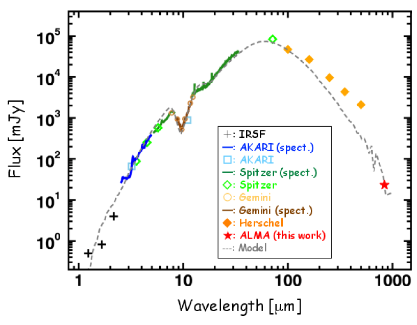
Figure 10: The spectral energy distribution of ST11. The plotted data are based on IRSF/SIRIUS photometry (pluses, black), AKARI/IRC spectroscopy (solid line, blue), AKARI/IRC photometry (open squares, light blue), Spitzer/MIPS spectroscopy (solid line, green), Spitzer/IRAC and MIPS photometry (open diamonds, light green), Gemini/T-ReCS narrow-band photometry (open circles, light brown), Gemini/T-ReCS N-band spectroscopy (solid line, brown), Herschel/PACS and SPIRE photometry (filled diamonds, orange), ALMA 840 $\mu$m continuum (filled star,red), and the best fitted SED model (dashed line, grey). See section $\S$ 4.5 for details.

Table 4: Photometric and spectroscopic data of ST11

Instrument	Wavelength	Flux	FWHM	Ref.
	($\mu$m)	(mJy)	($\arcsec$)
IRSF/SIRIUS J	1.23	0.50 $\pm$ 0.07	1.3	1
IRSF/SIRIUS H	1.66	0.82 $\pm$ 0.06	1.2	1
IRSF/SIRIUS Ks	2.16	3.98 $\pm$ 0.22	1.1	1
AKARI/IRC NG	2.5-5	spectroscopy	7.3	2
AKARI/IRC N3	3.2	66.0 $\pm$ 2.6	4.0	3
Spitzer/IRAC Band 1	3.6	88.1 $\pm$ 6.6	1.7	4
Spitzer/IRAC Band 2	4.5	252.2 $\pm$ 10.3	1.7	4
Spitzer/IRAC Band 3	5.7	577.8 $\pm$ 23.6	1.9	4
Spitzer/IRAC Band 4	7.9	1090.0 $\pm$ 39.7	2.0	4
AKARI/IRC S11	11	885.6 $\pm$ 29.7	4.8	3
Gemini-S/T-ReCS Si1	7.7	1329 $\pm$ 29	0.6	5
Gemini-S/T-ReCS Si2	8.7	940 $\pm$ 53	0.5	5
Gemini-S/T-ReCS Si3	9.7	523 $\pm$ 10	0.6	5
Gemini-S/T-ReCS Si4	10.4	950 $\pm$ 10	0.8	5
Gemini-S/T-ReCS Si5	11.7	2297 $\pm$ 12	0.8	5
Gemini-S/T-ReCS Si6	12.3	3226 $\pm$ 28	0.5	5
Gemini-S/T-ReCS Lo-Res	8–12	spectroscopy	0.7	5
Spitzer/IRS SL, SH, LH	5–36	spectroscopy	4-11	6
Spitzer/MIPS 70	70	83810 $\pm$ 1313	18	4
Herschel/PACS 100	100	47180 $\pm$ 3090	8.6	7
Herschel/PACS 160	160	26800 $\pm$ 1629	13	7
Herschel/SPIRE 250	250	9650 $\pm$ 589	18	7
Herschel/SPIRE 350	350	4359 $\pm$ 226	27	7
Herschel/SPIRE 500	500	2110 $\pm$ 151	41	7
ALMA Band 7	837	23.2 $\pm$ 2.32	0.5	5

Note. — ^aFWHM of the point spread function. ^bExtraction width of the slitless spectroscopic data. ^cSlit width.

References. — (1) Kato et al. (2007); (2) Shimonishi et al. (2010); (3) Kato et al. (2012); (4) Meixner et al. (2006); (5) This work; (6) Kemper et al. (2010); (7) Meixner et al. (2013)

5 Discussions

5.1 Hot molecular core associated with ST11

Hot cores are one of the early stages of high-mass star formation. It is suggested that the hot cores are in a transitional evolutionary stage between a deeply embedded protostellar object and a zero-age main-sequence star with a compact H II region (e.g., Zinnecker & Yorke, 2007). Physical properties of hot cores are characterized by a small source size ($\leq$0.1 pc), a high density ($\geq$10⁶ cm^-3), and warm gas/dust temperature ($\geq$100 K) (e.g., Kurtz et al., 2000; van der Tak, 2004). In this section, we discuss the presence of a hot core around ST11 on the basis of its physical and spectral properties.

5.1.1 Source size

A source size of ST11, which is measured by detected emission lines, is consistent with those of Galactic hot cores. The molecular lines of NO, SiO, ³³SO, SO₂, ³⁴SO₂, and ³³SO₂ as well as dust continuum show a compact source size, which is equal to or lower than the beam size of $\sim$0.1 pc. The lines of CO, C¹⁷O, HCO⁺, H¹³CO⁺ and H₂CO show somewhat extended distributions, but the dominant emission come from the compact region associated with a high-mass YSO. The extended components of these emission lines may arise from their relatively low critical densities and/or efficient formation routes in gas-phase reactions. Protostellar outflows, which is discussed in $\S$ 5.3, could also affect the spatial distribution of these molecular gas.

The spatial association of the molecular emission lines to the infrared source is another key to the nature of detected warm and dense molecular gas. Separation between a hot core region and an infrared source is reported to be smaller than $\sim$0.03 pc for typical Galactic sources (De Buizer et al., 2003). With the present spatial resolution, the distribution of molecular lines and dust continuum should coincide if they arise from a hot core region. This is clearly observed in the present data as shown in Figure 4.

5.1.2 Density

The H₂ gas density around ST11 is estimated to be $>$2 $\times$ 10⁶ cm^-3 in $\S$ 4.4. The value is a lower limit and actually clear detections of molecular lines with high critical densities such as those of SO₂ ($n_{cr}$ $\sim$10⁷ cm^-3, Williams & Viti, 2013) imply an even higher gas density around ST11. Galactic hot cores typically show gas densities between 10⁶–10⁸ cm^-3 (estimated from Tab.1 presented in Kurtz et al., 2000). The gas density around ST11 is thus consistent with those of known hot cores.

5.1.3 Gas temperature

Rotational temperatures of molecular gas around ST11 are compared with those of Galactic hot cores in Table 4.3. The temperature of SO₂, $T_{rot}$ = 195 $\pm$ 5 K, is in good agreement with temperatures of three Galactic hot cores in the table, which are between 108 K and 284 K. The temperature of ³⁴SO₂, $T_{rot}$ = 95 $\pm$ 7 K, is somewhat lower than that of SO₂, but this may be attributed to the combined effect of the lack of available higher excitation lines of ³⁴SO₂ and slightly larger optical thickness of SO₂ lines. Note that the temperature of ³³SO₂ is even lower, but this is probably because the detected lines are biased to those with low excitation temperatures ($E_{u}$ $<$ 200 K) due to the limited frequency coverage of the data. The rotation analysis of ³⁴SO₂ and ³³SO₂ for the Orion data using the similar set of lines with those used in the analysis of ST11 results in $T_{rot}$ = 114 $\pm$ 6 K for ³⁴SO₂ and $T_{rot}$ = 73 $\pm$ 5 K for ³³SO₂, which are lower than the values derived by Schilke et al. (1997) using a larger number of lines with a wide range of upper state energies (Tab. 4.3). Therefore we conclude that the actual temperature of SO₂ gas is in the order of $\sim$100 K, which can trigger hot core chemistry via sublimation of ice mantles. Sublimation of ice mantles around ST11 is also suggested from the infrared observations of ices in Shimonishi et al. (2010), which reported that ST11 shows the second weakest ice absorption bands among 12 high-mass YSOs in the LMC.

5.1.4 Central Protostar

As estimated in $\S$ 4.5, the bolometric luminosity (5 $\times$ 10⁵ L_☉) and stellar mass (50 M_☉) of ST11 are consistent with the properties of high-mass YSOs. This indicates that ST11 can form a hot core region with the help of its intense radiation. In addition, the red SED of ST11 (Fig. 10) indicates that it is still in an early evolutionary stage, which is consistent with the properties of hot core sources.

5.1.5 Spectral properties

Velocity widths of emission lines from ST11 are typically 4–7 km/s except for CO and HCO⁺. This is in good agreement with velocity widths of emission lines from Galactic hot core regions (typically 4–10 km/s, e.g., Helmich & van Dishoeck, 1997). Systemic velocities of the lines are in a very narrow range, typically 250–251 km/s, which suggests that the detected molecular species spatially coexist in a small region around a high-mass YSO.

SO₂ is often detected in hot core sources and one of the useful tracers of warm and dense gas around a high-mass YSO (e.g., Beuther et al., 2009). However, sometimes warm SO₂ gas is also prominently detected in deeply embedded and even younger protostellar objects in which hot cores are not yet formed (e.g., W3 IRS5 in Helmich et al., 1994). The reason of such SO₂ enhancement is suggested to be due to shock dominated chemistry triggered by protostellar outflows. These deeply embedded sources often show a deep self-absorption profile in their CO or HCO⁺ emission lines due to the presence of a significant amount of cold gas in the envelope. As shown in Figure 5, emission from ST11 does not show such a deep self-absorption profile. This suggests that emission from ST11 is mostly dominated by warm gas and that ST11 has already reached the hot core phase.

On the other hand, relatively weak strengths of hydrogen recombination lines seen in the near-infrared spectrum of ST11 suggests that a prominent H II region is not yet formed around the source (see Fig.1 in Shimonishi et al., 2010). Such a transitional evolutionary phase is well consistent with the properties of hot cores.

In summary, the compact size of the emitting source, the presence of warm and dense molecular gas around a high-mass protostar, the sublimation of ice mantles, and the detections of rich molecular lines suggest that ST11 is associated with a hot molecular core. This is the first detection of an extragalactic hot molecular core. Note that CH₃OH and complex organic molecules, which are often detected in Galactic hot cores, are not detected in ST11. The reason for the lack of these molecular species is discussed in the next section in the context of characteristic hot core chemistry in low metallicity.

5.2 Molecular abundances

Hot cores play a key role in the chemical complexity of interstellar and circumstellar molecules. In this section, we compare the chemical compositions of ST11 with those of Galactic hot cores and discuss the impact of metallicity on chemical processes in hot cores.

Fractional abundances of molecules around ST11 are shown in Table 5.2. We use the following isotope abundances for ST11; ¹²C/¹³C = 49, ¹⁶O/¹⁷O = 3400, and ³²S/³⁴S = 15, according to Wang et al. (2009) in which isotope ratios for the star-forming region N113 in the LMC are reported. For ³³S, we use ³²S/³³S = 40, which is estimated in this work (see $\S$ 5.2.12). For a comparison purpose, the table also includes the abundances of three Galactic hot cores, Orion, W3 (H₂O), and G34.3+0.15. Their abundances are re-estimated using the following isotope ratios of the local ISM and the Sun: ¹²C/¹³C = 77, ¹⁶O/¹⁷O = 1800, ³²S/³⁴S = 22, and ³²S/³³S = 127, according to Wilson & Rood (1994) and Anders & Grevesse (1989). All the abundances are estimated from the 345 GHz region data, except for NO in Orion, which is estimated using the transitions near 150 GHz.

Since ST11 is observed with the beam size of 0.12 pc, we here compare the abundances which are derived from the data with similar beam sizes. For Orion, we calculate the average abundance of five regions around the hot core (hot core, compact ridge, extended ridge, northwest plateau, and southeast plateau) using the data presented in Sutton et al. (1995). The abundances of NO and HNCO in Orion are only for the central part of the hot core and the data are adopted from Ziurys et al. (1991) and Schilke et al. (1997), respectively. The averaged Orion abundances roughly reproduce the abundances observed for the $\sim$0.08 pc region in diameter. The beam sizes of W3 (H₂O) and G34.3+0.15 correspond to 0.13 pc and 0.21 pc, respectively. We here assume the distances to Orion, W3 (H₂O), and G34.3+0.15 to be 0.41 kpc, 1.95 kpc, and 3.1 kpc (MacDonald et al., 1996; Reid et al., 2009).

Figure 11 compares fractional abundances of ST11 and Galactic hot cores. In general, most of the molecular species in ST11 show lower abundances compared to Galactic hot cores. Several molecules such as H₂CO, CH₃OH, HNCO, and CS show significantly lower abundances, which can not be simply explained by the low abundances of heavy elements in the LMC. On the other hand, NO shows the higher abundance in ST11 than in Galactic sources despite the notably low nitrogen abundance in the LMC. Characteristics of individual molecules are discussed below.

Table 5: Fractional abundances

	$N$(X)/$N$(H2)
Molecule	ST11	Orion	W3 (H2O)	G34.3+0.15	Note
CO	9.1 $\pm$ 0.7 $\times$ 10-5	6.9 $\times$ 10-5	1.9 $\times$ 10-4	$>$4.1 $\times$ 10-5	1
HCO+	7.5 $\pm$ 0.7 $\times$ 10-10	1.2 $\times$ 10-9	3.1 $\times$ 10-9	$>$1.7 $\times$ 10-9	2
H2CO	2.2 $\pm$ 0.2 $\times$ 10-10	2.9 $\times$ 10-8	4.2 $\times$ 10-9	$>$3.2 $\times$ 10-10
CH3OH	$<$8 $\times$ 10-10	1.8 $\times$ 10-7	9.2 $\times$ 10-8	3.4 $\times$ 10-8
NO	2.0 $\pm$ 0.6 $\times$ 10-8	1.1 $\times$ 10-8	$\cdots$	$>$1.1 $\times$ 10-8
HNCO	$<$1 $\times$ 10-10	1.6 $\times$ 10-9	5.0 $\times$ 10-9	$>$4.3 $\times$ 10-10
HC3N	$<$4 $\times$ 10-11	3.1 $\times$ 10-9	1.6 $\times$ 10-10	$>$3.6 $\times$ 10-11
SiO	3.3 $\pm$ 0.2 $\times$ 10-11	4.9 $\times$ 10-9	6.1 $\times$ 10-10	$>$2.3 $\times$ 10-11
CS	$<$3 $\times$ 10-10	8.3 $\times$ 10-9	9.9 $\times$ 10-9	$>$2.7 $\times$ 10-9	3
H2CS	6.2 $\pm$ 2.0 $\times$ 10-11	9.3 $\times$ 10-10	1.6 $\times$ 10-9	2.3 $\times$ 10-9
SO	2.4 $\pm$ 0.8 $\times$ 10-8	2.0 $\times$ 10-7	1.3 $\times$ 10-8	$>$5.0 $\times$ 10-9	4
SO2	2.1 $\pm$ 0.3 $\times$ 10-8	1.2 $\times$ 10-7	5.5 $\times$ 10-8	3.6 $\times$ 10-8	5
CH3OCH3	$<$3$\times$ 10-9	9.1 $\times$ 10-9	2.1 $\times$ 10-8	$\cdots$
HCOOCH3	$<$2 $\times$ 10-8	1.6 $\times$ 10-8	7.0 $\times$ 10-9	3.0 $\times$ 10-8
C2H5OH	$<$5 $\times$ 10-9	8.6 $\times$ 10-10	$\cdots$	6.6 $\times$ 10-9

Note. — Uncertainties and upper limits are of 2 $\sigma$ level and do not include systematic errors due to adopted spectroscopic constants. See $\S$ 5.2 for details of the data. (1) Estimated from C¹⁷O. (2) Estimated from H¹³CO⁺ except for Orion, which is estimated from HC¹⁸O⁺. (3) Estimated from C³⁴S. (4) Estimated from ³⁴SO, except for ST11, which is estimated from ³³SO. (5) Estimated from ³⁴SO₂.

References. — ^aThis work; ^bZiurys et al. (1991); Sutton et al. (1995); Schilke et al. (1997), also see $\S$ 5.2; ^cHelmich & van Dishoeck (1997); ^dMacDonald et al. (1996)

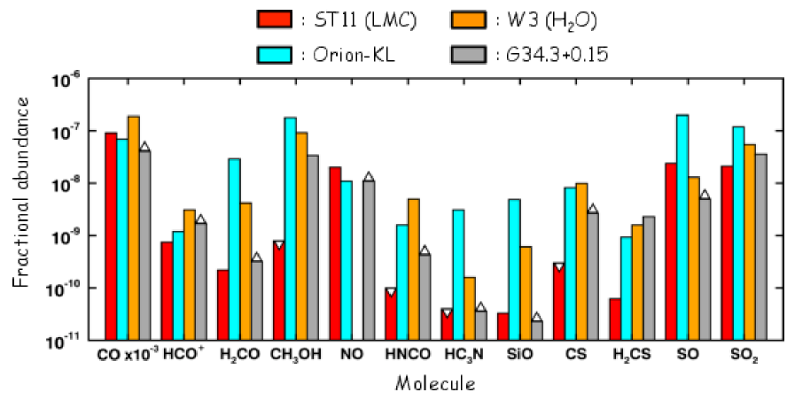
Figure 11: Molecular abundances of CO, HCO⁺, H₂CO, CH₃OH, NO, HNCO, HC₃N, SiO, CS, H₂CS, SO, and SO₂ for ST11 in the LMC (red) and Galactic hot cores, Orion hot core (cyan), W3 H₂O (orange), and G34.3+0.15 (grey). The downward and upward triangles represent the upper and lower limits, respectively. The plotted data are summarized in Table 5.2.

5.2.1 CO

Carbon monoxide is detected by the CO(3–2) and C¹⁷O(3–2) lines in ST11. The line intensity ratio of CO(3–2)/C¹⁷O(3–2) is about 28, and using ¹⁶O/¹⁷O = 3400 in the LMC (Wang et al., 2009) we estimate optical depths of $\sim$120 and $\sim$0.04 for CO(3–2) and C¹⁷O(3–2), respectively. The CO(3–2) line is completely optically thick, while the C¹⁷O(3–2) line is optically thin as in most of Galactic hot cores (e.g., Helmich & van Dishoeck, 1997). The abundance of CO in ST11 estimated from C¹⁷O is 9.1 $\times$ 10^-5, which is very similar to the average CO abundance of 1.0 $\times$ 10^-4 for three Galactic hot cores in Table 5.2. Elemental carbon and oxygen are about three times less abundant in the LMC; [C/H]_LMC = 1.2 $\times$ 10^-4 and [O/H]_LMC = 2.3 $\times$ 10^-4 (Korn et al., 2002), while [C/H]_☉ = 3.3 $\times$ 10^-4 and [O/H]_☉ = 6.8 $\times$ 10^-4 (Grevesse & Sauval, 1998). Given the low abundances of carbon and oxygen in the LMC, the CO around ST11 is slightly overproduced as compared with Galactic hot cores.

5.2.2 HCO⁺

Formyl ion is detected via the HCO⁺(4–3) and H¹³CO⁺(4–3) lines. The line intensity ratio of HCO⁺(4–3)/H¹³CO⁺(4–3) is about 19, and using ¹²C/¹³C = 49 in the LMC (Wang et al., 2009) we estimate optical depths of $\sim$2 and $\sim$0.05 for HCO⁺(4–3) and H¹³CO⁺(4–3), respectively. The HCO⁺(4–3) line is moderately optically thick, while the H¹³CO⁺(4–3) line is optically thin. The abundance of HCO⁺ in ST11 estimated from H¹³CO⁺ is 7.5 $\times$ 10^-10, which is lower by a factor of $\sim$3 compared to the average HCO⁺ abundance of 2.0 $\times$ 10^-9 for three Galactic hot cores in Table 5.2.

We here discuss the connection between the observed HCO⁺ abundance and the cosmic-ray ionization rate in the LMC. One of the possible pathways to form HCO⁺ in molecular clouds is the gas-phase reaction:

$$\mathrm{H_{3}^{+}+CO\to HCO^{+}+H_{2},}$$ (8)

in which H${}_{3}^{+}$ is formed by ionization of H₂ via cosmic rays and subsequent reaction with H₂ (e.g., Caselli et al., 1998).

We here simply assume that HCO⁺ is a major cation and electron is a major anion in dense clouds. Given that production of cations and electrons by the cosmic-ray ionization balances with their recombination, the equilibrium is formulated as

$$\zeta n_{\mathrm{H_{2}}}=k_{rec}n_{\mathrm{HCO^{+}}}n_{e},$$ (9)

where $\zeta$ is a cosmic-ray ionization rate, $k_{rec}$ = 2.4 $\times$ 10^-7 (300/$T$)^0.69 cm³ s^-1 (5.1 $\times$ 10^-7 at $T$ = 100 K) is a dissociative recombination rate of HCO⁺ and electron (Mitchell, 1990), $n$ indicates a number density of each species. With the assumption that cations and electrons have the the same abundance in neutral clouds, this equation is reformatted as

$$X_{HCO^{+}}=X_{e}=\sqrt{\zeta/n_{H_{2}}k_{rec}},$$ (10)

where $X$ indicates a fractional abundance relative to H₂. This equation indicates that the abundance of HCO⁺ is proportional to $\zeta^{0.5}$ under the above simple assumption.

The cosmic-ray density in the LMC is reported to be 20–30$\%$ of the typical Galactic value of $\zeta$ = 3 $\times$ 10^-17 s^-1 based on gamma-ray observations (Abdo et al., 2010). The low cosmic-ray density leads to the low cosmic-ray ionization rate (e.g., Spitzer & Tomasko, 1968). According to Eq. 10, the HCO⁺ abundance in the LMC is expected to be lower than the Galactic value by a factor of $\sim$2 for the same H₂ density and gas temperature. This factor is close to the observed difference of the HCO⁺ abundance between ST11 and Galactic sources. Therefore, we speculate that the low cosmic-ray ionization rate in the LMC is one of the factors that contribute to the slightly low abundance of HCO⁺ in ST11.

Note that the above assumption is very simple; i.e., the cosmic-ray ionization rate may vary within the LMC and the electron abundance may differ from that of HCO⁺ due to the presence of other ions. Furthermore, in the above discussion, we consider only one of the possible mechanisms to form HCO⁺. In a circumstellar environment of hot cores, however, outflows and stellar radiation would affect the ionization condition. Previous studies actually argue that molecular outflows and shocks contribute to the enhancement of HCO⁺ in star-forming cores (e.g., Girart et al., 1999; Rawlings et al., 2004; Arce & Sargent, 2006). Future observations of other molecular ions and shock tracers are highly required for comprehensive understanding of ionization conditions in the LMC.

5.2.3 H₂CO

Formaldehyde (H₂CO) is detected by the 5_1,5–4_1,4 transition at 351.7686 GHz ($E_{u}$ = 62 K). The abundance of H₂CO in ST11 is estimated to be 2.2 $\times$ 10^-10, while Galactic hot cores show the abundances between 10^-9 to 10^-8 as in Table 5.2, except for G34.3+0.15 which only has a lower limit. The H₂CO is less abundant in ST11 than Galactic sources by 1–2 orders of magnitude.

Both gas-phase and grain surface reaction pathways are suggested for the formation of H₂CO in dense ISM. The grain surface pathway for the H₂CO formation requires the hydrogenation of CO (e.g., Hama & Watanabe, 2013, and references therein). However, this pathways is suppressed in the LMC due to higher dust temperatures (see detailed discussion presented in $\S$ 5.2.4). Therefore we speculate that suppressed formation of the H₂CO ice on grain surfaces contributes to the low abundance of H₂CO gas in ST11.

5.2.4 CH₃OH

Any of methanol (CH₃OH) lines is not detected in ST11. We estimate an upper limit on the fractional abundance to be $<$8 $\times$ 10^-10 using the spectrum at the frequency of the CH₃OH(7₀–6₀ A⁺) transition at 338.4087 GHz ($E_{u}$ = 65 K). Abundances of CH₃OH in Galactic hot cores are typically between $\sim$10^-8 to $\sim$10^-7 as in Table 5.2, but sometimes the abundance reaches $\sim$10^-6 (e.g., G5.89-0.39 in Thompson & MacDonald, 1999). In ST11, CH₃OH is depleted by at least 2–3 orders of magnitude as compared with Galactic hot cores.

The low abundance of CH₃OH in the LMC has been suggested in previous studies. Nishimura et al. (2016) reported, based on spectral line surveys toward molecular clouds in the LMC, that thermal emission lines of CH₃OH gas are significantly weak in the LMC compared to our Galaxy. Searches for maser emission in the LMC reported the underabundance of CH₃OH masers in the LMC (e.g., Ellingsen et al., 2010). Furthermore, Shimonishi et al. (2016) reported that the CH₃OH ice is less abundant in the LMC than in our Galaxy based on infrared observations. They reported that all of the observed ten high-mass YSOs in the LMC show CH₃OH ice abundances less than 5–8 $\%$ relative to water ice, while about one-third of Galactic high-mass YSOs show CH₃OH ice abundances between 10 $\%$ and 40 $\%$. The authors suggested that warm ice chemistry is responsible for the low abundance of solid CH₃OH in the LMC; i.e., high dust temperatures in the LMC suppress the hydrogenation of CO on the grain surface, which leads to inefficient production of the CH₃OH ice. A decrease in the efficiency of CO hydrogenation at an elevated temperature is measured by laboratory experiments (e.g., Watanabe et al., 2003). In addition, the reduced formation of CH₃OH in relatively warm molecular clouds is confirmed by numerical simulations of grain surface chemistry dedicated to the LMC environment (Acharyya & Herbst, 2015).

The warm gas temperature around ST11 suggests that ice mantles are mostly sublimated. The low elemental abundances of carbon and oxygen in the LMC should partly contribute to the observed low CH₃OH abundance. However, we need additional explanation to account for the CH₃OH deficiency by several orders of magnitude, and this should be related to grain surface chemistry by which CH₃OH is mainly formed. We suggest that suppressed production of CH₃OH ice due to warm ice chemistry at the molecular cloud stage or the deeply embedded YSO stage is responsible for the deficiency of CH₃OH gas in this LMC hot core.

The above interpretation on the low CH₃OH abundance can also be applied to the low abundance of H₂CO in ST11 since a major grain surface pathway of both species requires the CO hydrogenation. However, the difference is that H₂CO has possible formation routes both in the gas-phase and in the solid-phase, while CH₃OH does not have an efficient formation route in the gas-phase under typical molecular cloud conditions. We speculate that the H₂CO observed in ST11 is mainly produced by gas-phase reactions. A slightly extended distribution of the H₂CO emission (Fig. 4) supports this idea, because the species sublimated from ice mantles often show the compact distribution compared to those produced in the gas phase. Owing to the lack of a possible gas-phase formation route, the degree of depletion around ST11 is actually larger in CH₃OH as compared to H₂CO.

5.2.5 NO

Nitric oxide (NO) is one of the interesting molecules that show a peculiar abundance in ST11. The abundance of NO in ST11 is estimated to be 2.0 $\times$ 10^-8. On the other hand, the average abundance and standard deviation of NO in six Galactic sources in Ziurys et al. (1991) including hot cores, high-mass protostellar objects, and Galactic center objects is 8.2 $\pm$ 2.9 $\times$ 10^-9. In the LMC, nitrogen is even more depleted than other major elements such as carbon and oxygen; the elemental abundance of nitrogen in the LMC is [N/H]_LMC = 1.0 $\times$ 10^-5 (Korn et al., 2002), while [N/H]_☉ = 8.3 $\times$ 10^-5 for the Sun (Grevesse & Sauval, 1998). Despite the lower nitrogen abundance by a factor of 8 in the LMC, the abundance of NO in ST11 is higher than Galactic star-forming regions by a factor of 2–3.

Ammonia (NH₃) gas, which is often the most abundant nitrogen-bearing species in star-forming regions, is reported to be deficient in the LMC by 1.5–2 orders of magnitude as compared with Galactic star-forming regions (Ott et al., 2010). A previous infrared study suggests that the NH₃ ice around an embedded high-mass YSO in the LMC is possibly less abundant as compared with Galactic high-mass YSOs (Shimonishi et al., 2016). Although the NH₃ abundance in ST11 is unknown, the relatively high abundance of NO implies that NO could play an important role in nitrogen chemistry around ST11.

It is suggested that NO is formed by a neutral-neutral reaction in the gas-phase (e.g., Herbst & Klemperer, 1973; Pineau des Forets et al., 1990):

$$\mathrm{N+OH\to NO+H,}$$ (11)

and destroyed by

$$\mathrm{NO+N\to N_{2}+O.}$$ (12)

A numerical simulation of nitrogen chemistry in warm molecular gas suggests that the resultant abundance of NO through the above reactions increases as the temperature of molecular gas increases (Pineau des Forets et al., 1990). However, the enhancement of the NO abundance is suggested to be only a factor of 1.5 as the gas temperature increases from 70 K to 250 K. Thus we speculate that pure gas-phase chemistry make only a limited contribution on the enhanced abundance of NO in ST11.

A compact distribution of the NO emission observed in ST11 may hint at the possible origin in ice sublimation. Laboratory experiments argue that bombardment of energetic ions to interstellar ice analogues containing H₂O, O₂, and N₂ or CO and N₂ produce NO in ice mixtures (Boduch et al., 2012; Sicilia et al., 2012). However, the low cosmic-ray density in the LMC (see $\S$ 5.2.2) implies that the formation of NO by such energetic processing is less efficient around ST11. A reaction pathway though diffusive grain surface chemistry, N + O $\to$ NO, is also suggested in the literature (Tielens & Hagen, 1982), but uncertainty remain regarding the efficiency of the reaction in actual grain surfaces.

The reason of the enhanced abundance of NO in ST11 despite the low elemental abundance of nitrogen in the LMC remains to be investigated. Detailed modeling of hot core chemistry in metal-poor environments is obviously necessary to interpret the enhanced abundance of NO in ST11.

5.2.6 HNCO

Isocyanic acid (HNCO) is not detected in ST11. We estimate an upper limit on the fractional abundance of HNCO to be $<$1 $\times$ 10^-10 based on the non-detection of the 16_0,16–15_0,15 transition at 351.6333 GHz ($E_{u}$ = 143 K). There seems to be an emission-like feature at the position of the HNCO(16_3,14–15_3,13 and 16_3,13–15_3,12, 351.4168 GHz) line with $V_{LSR}$ = 250.8 km/s. However, the high upper state energy of this transition ($E_{u}$ = 518 K) and the non-detection of the 16_0,16–15_0,15 transition suggest that this line is likely a spurious signal. Galactic hot cores and high-mass protostellar objects typically show the HNCO abundances between 10^-9 to 10^-8 (Bisschop et al., 2007), which is consistent with the average abundance of 2.3 $\times$ 10^-9 for three Galactic hot cores in Table 5.2. Thus the HNCO abundance in ST11 is lower than Galactic counterparts by at least 1–2 orders of magnitude.

Both gas-phase and grain surface reaction pathways are suggested for the formation of HNCO in dense ISM (e.g., Tielens & Hagen, 1982; Turner et al., 1999). The grain surface pathway requires the hydrogenation of CO to form HCO and subsequent reaction of HCO + N $\to$ HNCO. However, as discussed in $\S$ 5.2.4, the hydrogenation of CO is suggested to be less efficient in the LMC due to high dust temperatures, which possibly suppress the grain surface formation of HNCO. This may contribute to the low abundance of HNCO in ST11 along with the low elemental abundance of nitrogen in the LMC.

5.2.7 HC₃N

Cyanoacetylene (HC₃N), an unsaturated carbon-chain molecule often detected in star-forming regions, is not detected in ST11. We estimate an upper limit on the fractional abundance of HC₃N to be $<$4 $\times$ 10^-11 based on the non-detection of the 38–37 transition at 345.6090 GHz ($E_{u}$ = 323 K). Abundances of HC₃N in Galactic hot cores vary from $\sim$10^-11 to $\sim$10^-9 as in Table 5.2. The estimated upper limit on the HC₃N abundance in ST11 is thus at the lower end of the Galactic HC₃N abundance.

5.2.8 SiO

Silicon monoxide (SiO) is detected by the J = 8–7 transition at 347.3306 GHz ($E_{u}$ = 75 K). The abundance of SiO for ST11 is 3.3 $\times$ 10^-11, which seems to be low compared to Galactic sources, but the dispersion in the Galactic SiO abundances is significantly large as shown in Figure 11. The average SiO abundance for the three Galactic hot cores in Table 5.2 is 1.8 $\times$ 10^-9, but their abundances range from $\sim$10^-11 to $\sim$10^-9.

The elemental abundance of silicon in the LMC is about three times lower than the solar abundance; [Si/H]_LMC = 1.3 $\times$ 10^-5 (Korn et al., 2002), while [Si/H]_☉ = 3.6 $\times$ 10^-5 (Grevesse & Sauval, 1998). Thus the elemental abundance in the LMC partly contributes to the observed low SiO abundance, but additional processes may be necessary to account for the 1–2 orders of magnitude lower SiO abundance.

SiO is often linked with the presence of energetic protostellar outflows since destruction of silicon-bearing dust (e.g., MgSiO₃) by shock is believed to be the origin of SiO (e.g., Blake et al., 1996; Wright et al., 1996; Tercero et al., 2011, and references therein). Destruction of dust grains and release of silicon can occur around ST11 since it shows a sign of outflows as described in $\S$ 5.3. On the other hand, the low abundance of SiO would imply that shock chemistry is not very dominant in the present chemical compositions around ST11. Further quantitative discussions require detailed modeling of SiO production in low metallicity environments. Various factors including the degree of shock, elemental abundances, and compositions of dust grains may affect the SiO abundance.

5.2.9 CS

The C³⁴S(7–6) transition at 337.3965 GHz ($E_{u}$ = 65 K) is not detected toward ST11. We estimate an upper limit on the abundance of carbon monosulfide (CS) to be $<$3 $\times$ 10^-10, while Galactic hot cores and high-mass protostellar objects typically show the CS abundances between 10^-9 and 10^-8 (Tab. 5.2, see also van der Tak et al., 2003). CS is significantly less abundant by at least 1–2 orders of magnitude in ST11 compared to Galactic sources, and the low elemental abundances of carbon and sulfur in the LMC can not by itself explain the depletion of CS. Given the relatively high abundance of SO₂ in ST11 as discussed in $\S$ 5.2.12, a significant amount of gas-phase sulfur is possibly incorporated in SO₂ due to different circumstellar chemistry around ST11.

5.2.10 H₂CS

We detect the emission line of thioformaldehyde (H₂CS) at 338.0832 GHz (10_1,10–9_1,9, $E_{u}$ = 65 K), but the S/N of the line is relatively poor. The H₂CS abundance is estimated to be 6.2 $\times$ 10^-11 in ST11, while Galactic hot cores show the abundance of $\sim$2 $\times$ 10^-9 on average with a relatively low dispersion (Tab. 5.2). H₂CS seems to be less abundant in the LMC hot core than in Galactic hot cores as well as CS, and only a small fraction of gas-phase sulfur is incorporated into H₂CS in ST11. Since our H₂CS abundance is estimated using a single line with poor S/N, further multi-line observations of H₂CS transitions are necessary for accurate determination of the H₂CS abundance in the LMC.

5.2.11 SO

The abundance of sulfur monoxide (SO) is estimated to be 2.4 $\times$ 10^-8 in ST11, while Galactic hot cores and high-mass protostellar objects typically show the SO abundances between 10^-9 and 10^-8 (Tab. 5.2, see also van der Tak et al., 2003). The Orion hot core shows an exceptionally high SO abundance of 2.0 $\times$ 10^-7. The results suggest that ST11 shows a slightly higher abundance of SO than typical Galactic counterparts despite the low metallicity of the LMC. If we use the solar ³²S/³³S ratio of 127, then the SO abundance in ST11 is 7.6 $\times$ 10^-8, which is even higher than typical Galactic abundances.

We emphasize, however, that our SO abundance entails considerable uncertainty. The abundance is estimated using a single ³³SO line at 337.1986 GHz ($E_{u}$ = 81 K), which contains a number of unresolved hyperfine structures, while Galactic SO abundances are estimated from ³⁴SO lines. Multi-line observations of SO and its isotopologues are necessary for further discussion.

5.2.12 SO₂

Sulfur dioxide (SO₂) is in this study a key molecule for which we detect the largest number of transitions; we detect nine SO₂ lines, one SO₂ ($\nu$₂=1) line, ten ³⁴SO₂ lines, and five ³³SO₂ lines. The fractional abundance of SO₂ is estimated to be 2.1 $\times$ 10^-8 in ST11 based on rotation diagram analysis of ³⁴SO₂ lines. The column density ratio of SO₂ and ³⁴SO₂ is about 14, suggesting that the optically thin assumption is mostly valid for the observed SO₂ lines because the ³²S/³⁴S ratio is reported to be 15 in the LMC. If we assume the solar isotope ratio of ³²S/³⁴S = 22, the SO₂ lines could be moderately optically thick. In either case, we can reasonably assume that ³⁴SO₂ and ³³SO₂ lines are optically thin because these isotopologues are much less abundant than ³²SO₂. The isotope abundance of ³³S in ST11 based on the present results is ³²S/³³S = 40, while the solar value is ³²S/³³S = 127.

Galactic hot cores typically show the SO₂ abundance from $\sim$10^-8 to $\sim$10^-7, while even younger embedded high-mass protostellar objects show the abundance of $\sim$10^-9 (van der Tak et al., 2003). ST11 shows a factor of $\sim$3 lower SO₂ abundance as compared with the average abundance of 7.0 $\times$ 10^-8 for the three Galactic hot cores in Table 5.2. The elemental abundance of sulfur in the LMC is reported to be [S/H]_LMC = 5.0 $\times$ 10^-6, while the solar abundance is [S/H]_☉ = 1.9 $\times$ 10^-5 (Russell & Dopita, 1992). Sulfur is less abundant by a factor of $\sim$4 in the LMC compared with the solar abundance. Thus, the low SO₂ abundance in ST11 is well explained by the elemental abundance of sulfur in the LMC. This would suggest that hot core chemistry of SO₂ is dependent on elemental abundances of the host galaxy. A multitude of SO₂ and its isotopologue line detections in ST11 imply that SO₂ can be a key molecular tracer to test hot core chemistry in metal-poor environments.

It should be noted that sulfur chemistry in hot core regions is highly time-dependent (e.g., Charnley, 1997). Hence, both the age and the interstellar environment should be taken into account to interpret the chemical compositions of sulfur-bearing species around ST11. Numerical simulations of hot core chemistry dedicated to low metallicity environments are thus highly required.

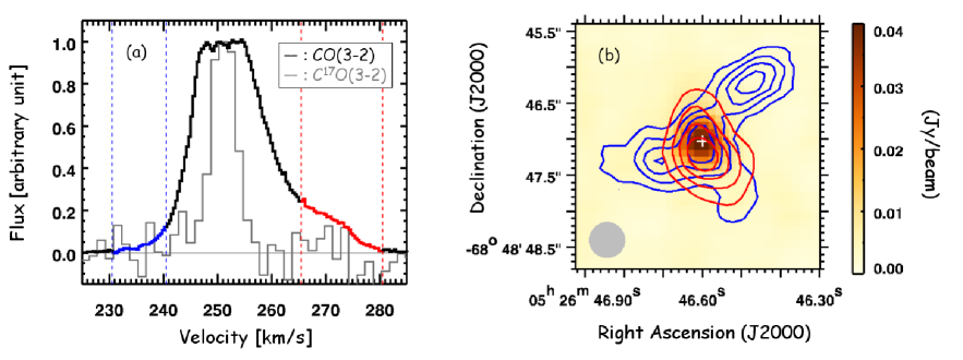
Figure 12: (a) Comparison of spectral line profiles of CO(3–2) (thick solid line, black) and C¹⁷O(3–2) (thin solid line, gray) observed toward ST11. The spectra are arbitrarily scaled and the horizontal axis is the LSR velocity. The CO line shows a broad line width and a prominent red-shifted component, which indicate the presence of outflows in the line of sight. The blue and red vertical dashed lines represent the velocity range of the blue-shifted and red-shifted high-velocity components, which are visualized in the right panel. (b) Spatial distributions of integrated intensities of high-velocity wings. The blue-shifted and red-shifted wing components are shown by the blue and red contours. The contour levels are 20 $\%$, 40 $\%$, 60 $\%$, and 80 $\%$ of the peak intensity. The background is the 840 $\mu$m continuum. The synthesized beam size is shown by the gray filled circle at the lower left.

5.2.13 CH₃OCH₃, HCOOCH₃, C₂H₅OH

Spectral lines from complex organic molecules are not detected in this work. We estimate upper limits on fractional abundances of three molecules whose relatively strong transitions are covered in the present data; [CH₃OCH₃/H₂] $<$3 $\times$ 10^-9, [HCOOCH₃/H₂] $<$2 $\times$ 10^-8, and [C₂H₅OH/H₂] $<$5 $\times$ 10^-9. Average abundances of these molecules for Galactic hot cores in Table 5.2 are [CH₃OCH₃/H₂] = 1.5 $\times$ 10^-8, [HCOOCH₃/H₂] = 1.8 $\times$ 10^-8, and [C₂H₅OH/H₂] $=$ 3.7 $\times$ 10^-9. These estimates suggest that CH₃OCH₃ is less abundant by at least an order of magnitude in ST11 compared with Galactic hot cores, while upper limit abundances of HCOOCH₃ and C₂H₅OH are comparable to the average abundances of Galactic sources. Although the present data do not provide conclusive upper limits on abundances of a majority of complex organic molecules in the LMC, the possibly lower abundance of CH₃OCH₃ in ST11 suggests the formation of large molecules may be less efficient in the LMC.

It is suggested by theoretical studies that CH₃OH in ice mantles plays an important role in the formation of complex organic molecules (e.g., Nomura & Millar, 2004; Garrod, 2008; Herbst & van Dishoeck, 2009). Shimonishi et al. (2016) argue that formation of complex organic molecules from methanol-derived species could be less efficient in the LMC due to the low abundance CH₃OH ice around high-mass YSOs in the LMC. We confirm the significant deficiency of CH₃OH gas around ST11 in this work. We thus speculate that the low abundance of CH₃OH contributes to the low production efficiency of CH₃OCH₃ and possibly other complex organic molecules in the LMC.

Note that unknown rotational temperatures and limited frequency coverages produce considerable uncertainties on the abundance estimate. Furthermore, the formation of large molecules from other parent species such as H₂CO, C₂H, c-C₃H₂, and NO, which are detected in the LMC, should be taken into account for comprehensive understanding of complex chemistry around protostars. Hence, further observations with broader frequency coverage and higher sensitivity are critically needed in conjunction with theoretical and experimental effort to understand complex organic chemistry in metal-poor environments.

5.3 Molecular outflows

In this section, we discuss the second detection of extragalactic protostellar outflows after Fukui et al. (2015), which reported the detection of protostellar outflows in the star-forming region N159 in the LMC with ALMA. Evidence of protostellar outflows is seen in the CO emission line of ST11. Figure 12(a) shows the spectral profile of the CO(3–2) line extracted from the 0.5$\arcsec$ diameter region centered at ST11. The profile of the optically thin C¹⁷O(3–2) line is also shown for a comparison purpose. The CO(3–2) profile shows an apparently broader velocity width compared to other lines detected in ST11. The central velocity of the CO line is nearly consistent with those of other lines ($V_{LSR}$ $\sim$250), but the emission distributes in a wide velocity range from 230 km/s to 280 km/s. In addition, a prominent red-shifted component is seen around $V_{LSR}$ $\sim$270 km/s. We suggest that these high-velocity wing components are due to protostellar outflows from ST11 because the high-velocity CO gas is well spatially associated with a high-mass YSO as described in the next paragraph. The observed outflow velocity of $\sim$10–30 km/s is consistent with molecular outflow velocities observed in Galactic high-mass star-forming regions (e.g., Lada, 1985). A high-velocity component is not obviously seen in other lines besides CO(3–2).

Spatial distributions of high-velocity wings are shown in Figure 12(b). We here define the velocity range of the blue-shifted wing to be 230.5 km/s to 240.5 km/s and the red-shifted wing to be 265.5 km/s to 285.5 km/s. Both high-velocity wings are spatially associated with a central protostar which is traced the the continuum emission. The complex structures seen in the distribution of high-velocity gas imply that the circumstellar environment of ST11 is dynamically active. If we assume the spatial extent of high-velocity gas to be 0.24 pc ($\sim$1$\arcsec$) and the outflow velocity to be 20 km/s according to the distribution and spectrum of the red wing component, we can roughly estimate an upper limit on the dynamical timescale of the outflow, which is about 10⁴ years. This timescale is lower than a typical formation time of high-mass stars ($\sim$10⁵ years, Zinnecker & Yorke, 2007) and thus consistent with high-mass star-formation scenarios.

We also make a rough estimate of several outflow parameters, namely, the outflow mass, the mass entrainment rate, the mechanical force, and the energy. The outflow mass is estimated by adding blue and red wing components within the region where outflow gas emission is detected with the S/N ratio higher than six. To convert integrated intensities of CO(3–2) to the total gas mass, we use a conversion factor of 8.8 M_☉ (K km/s)^-1 pc^-2, which is derived from the present observations toward the ST11 center. The derived outflow mass is $M_{\mathrm{out}}$ = 74 M_☉, where the blue-shifted component contains 13 M_☉ ($M_{\mathrm{blue}}$) and the red-shifted component contains 61 M_☉ ($M_{\mathrm{red}}$). This outflow mass corresponds to the mass entrainment rate of $\dot{M}=M_{\mathrm{out}}/t=$ 7 $\times$ 10^-3 M_☉ yr^-1, where $t$ is the dynamical time scale of outflows discussed above (10⁴ yr). The mechanical force ($F$) and the energy ($E$) of outflows are derived by the following equations: $F=(M_{\mathrm{blue}}V_{\mathrm{blue}}+M_{\mathrm{red}}V_{\mathrm{red}})/t$ and $E=(M_{\mathrm{blue}}V_{\mathrm{blue}}^{2}+M_{\mathrm{red}}V_{\mathrm{red}}^{2})/2$. $V_{\mathrm{blue}}$ and $V_{\mathrm{red}}$ are mean velocities of blue and red wing components, and we use $V_{\mathrm{blue}}$ = 13 km/s and $V_{\mathrm{red}}$ = 20 km/s, respectively. Consequently, the derived outflow force is $F$ = 0.14 M_☉ km/s yr^-1 and the outflow energy is $E$ = 3 $\times$ 10⁴⁷ erg. The above outflow parameters for ST11 are roughly consistent with those observed in Galactic high-mass YSOs that have similar luminosities with ST11 (e.g., Beuther et al., 2002).

The present detection increases the number of extragalactic protostellar outflow samples, which should help understand the dynamical processes of high-mass star-formation in different metallicity environments. Systematic observations of extragalactic outflow sources are necessary for statistical comparison of Galactic and extragalactic protostellar outflows. Further detailed analysis of outflows around ST11 is beyond the scope of this paper and will be presented in a future work.

6 Summary

We report the first detection of an extragalactic hot molecular core based on radio interferometric observations toward ST11, a high-mass YSO in the LMC, with ALMA. The high spatial resolution (0.12 pc) ALMA Band 7 (345 GHz) spectral and continuum band observation data are presented. We discuss the physical and chemical properties of the source and obtained the following conclusions.

1. Molecular emission lines of CO, C¹⁷O, HCO⁺, H¹³CO⁺, H₂CO, NO, SiO, H₂CS, ³³SO, ³²SO₂, ³⁴SO₂, and ³³SO₂ are detected from a compact region ($\sim$0.1 pc) associated with a high-mass YSO. Furthermore, a number of high excitation lines ($E_{u}$ $>$100 K) of SO₂ and its isotopologues are detected. On the other hand, CH₃OH, HNCO, CS, HC₃N, and complex organic molecules are not detected.

2. Physical properties of ST11 are derived using the obtained data. The H₂ gas density around the source is estimated to be at least 2 $\times$ 10⁶ cm^-3 based on the dust continuum data. The temperature of molecular gas is estimated to be higher than 100 K based on rotation diagram analysis of SO₂ and ³⁴SO₂ lines. The SED analysis in the 1–1000 $\mu$m range suggests that ST11 is a high-mass YSO with the luminosity of 5 $\times$ 10⁵ L_☉ and the stellar mass of 50 M_☉.

3. The compact size of the emitting source, warm gas temperature, high density, and rich molecular lines around a high-mass protostar suggest that ST11 is associated with a hot molecular core.

4. We find that the molecular abundances of the hot core in the LMC are significantly different from those of Galactic hot cores. The abundances of CH₃OH, H₂CO, and HNCO are remarkably lower compared with Galactic sources by at least 1–3 orders of magnitude, although the gas temperature is warm enough for the sublimation of ice mantles. The deficiency of CH₃OH gas in a warm and dense region is consistent with the previously reported low abundance of the CH₃OH ice in the LMC. We suggest that the chemical compositions of ST11 are characterized by the deficiency of molecules whose formation requires the hydrogenation of CO on grain surfaces.

5. It is interesting that NO shows a higher abundance in ST11 than in Galactic sources despite the notably low abundance of nitrogen in the LMC. This is in contrast to low abundances of nitrogen-bearing molecules such as NH₃, HCN, HNC in the LMC reported by previous studies. The reason of the enhanced abundance of NO remains to be investigated.

6. Slightly lower abundance of SO₂ in ST11 than in Galactic hot cores is well explained by the low abundance of elemental sulfur in the LMC. CS and H₂CS are less abundant than Galactic hot cores by at least 1–2 orders of magnitude. The abundance of SO is possibly high in the LMC, but the estimate based on a single ³³SO line should be taken with caution. The large number of SO₂ and its isotopologue line detections in the LMC hot core imply that SO₂ can be a key molecular species to test hot core chemistry in metal-poor environments.

7. We find molecular outflows around ST11, which is the second detection of an extragalactic protostellar outflow. An apparently broad velocity width is seen in the spectral profile of the CO(3–2) line, which ranges in the LSR velocity from 230 km/s to 280 km/s. A prominent high-velocity component is also seen in the red-shifted wing. We estimate an upper limit on the dynamical timescale of outflows to be 10⁴ years, which is consistent with the timescale of high-mass star formation. Several outflow parameters are also estimated based on the present results.

References

- Abdo et al. (2010) Abdo, A. A., Ackermann, M., Ajello, M., et al. 2010, A&A, 512, A7
- Acharyya & Herbst (2015) Acharyya, K., & Herbst, E. 2015, ApJ, 812, 142
- Anders & Grevesse (1989) Anders, E., & Grevesse, N. 1989, Geochim. Cosmochim. Acta, 53, 197
- Anderson et al. (2014) Anderson, C. N., Meier, D. S., Ott, J., et al. 2014, ApJ, 793, 37
- Arce & Sargent (2006) Arce, H. G., & Sargent, A. I. 2006, ApJ, 646, 1070
- Bernard et al. (2008) Bernard, J.-P., Reach, W. T., Paradis, D., et al. 2008, AJ, 136, 919
- Beuther et al. (2002) Beuther, H., Schilke, P., Sridharan, T. K., et al. 2002, A&A, 383, 892
- Beuther et al. (2009) Beuther, H., Zhang, Q., Bergin, E. A., & Sridharan, T. K. 2009, AJ, 137, 406
- Bisschop et al. (2007) Bisschop, S. E., Jørgensen, J. K., van Dishoeck, E. F., & de Wachter, E. B. M. 2007, A&A, 465, 913
- Blake et al. (1996) Blake, G. A., Mundy, L. G., Carlstrom, J. E., et al. 1996, ApJ, 472, L49
- Boduch et al. (2012) Boduch, P., Domaracka, A., Fulvio, D., et al. 2012, A&A, 544, A30
- Caselli et al. (1998) Caselli, P., Walmsley, C. M., Terzieva, R., & Herbst, E. 1998, ApJ, 499, 234
- Charnley (1997) Charnley, S. B. 1997, ApJ, 481, 396
- Chin et al. (1997) Chin, Y.-N., Henkel, C., Whiteoak, J. B., et al. 1997, A&A, 317, 548
- Cox (2000) Cox, A. N. 2000, Allen’s astrophysical quantities
- De Buizer et al. (2003) De Buizer, J. M., Radomski, J. T., Telesco, C. M., & Piña, R. K. 2003, ApJ, 598, 1127
- Ellingsen et al. (2010) Ellingsen, S. P., Breen, S. L., Caswell, J. L., Quinn, L. J., & Fuller, G. A. 2010, MNRAS, 404, 779
- Fukui et al. (2015) Fukui, Y., Harada, R., Tokuda, K., et al. 2015, ApJ, 807, L4
- Garrod (2008) Garrod, R. T. 2008, A&A, 491, 239
- Garrod & Herbst (2006) Garrod, R. T., & Herbst, E. 2006, A&A, 457, 927
- Garrod et al. (2008) Garrod, R. T., Weaver, S. L. W., & Herbst, E. 2008, ApJ, 682, 283
- Girart et al. (1999) Girart, J. M., Ho, P. T. P., Rudolph, A. L., et al. 1999, ApJ, 522, 921
- Goldsmith & Langer (1999) Goldsmith, P. F., & Langer, W. D. 1999, ApJ, 517, 209
- Grevesse & Sauval (1998) Grevesse, N., & Sauval, A. J. 1998, Space Sci. Rev., 85, 161
- Hama & Watanabe (2013) Hama, T., & Watanabe, N. 2013, Chemical Reviews, 113, 8783
- Heikkilä et al. (1999) Heikkilä, A., Johansson, L. E. B., & Olofsson, H. 1999, A&A, 344, 817
- Helmich et al. (1994) Helmich, F. P., Jansen, D. J., de Graauw, T., Groesbeck, T. D., & van Dishoeck, E. F. 1994, A&A, 283, 626
- Helmich & van Dishoeck (1997) Helmich, F. P., & van Dishoeck, E. F. 1997, A&AS, 124
- Herbst & Klemperer (1973) Herbst, E., & Klemperer, W. 1973, ApJ, 185, 505
- Herbst & van Dishoeck (2009) Herbst, E., & van Dishoeck, E. F. 2009, ARA&A, 47, 427
- Indebetouw et al. (2013) Indebetouw, R., Brogan, C., Chen, C.-H. R., et al. 2013, ApJ, 774, 73
- Israel et al. (1986) Israel, F. P., de Graauw, T., van de Stadt, H., & de Vries, C. P. 1986, ApJ, 303, 186
- Johansson et al. (1994) Johansson, L. E. B., Olofsson, H., Hjalmarson, A., Gredel, R., & Black, J. H. 1994, A&A, 291, 89
- Kato et al. (2007) Kato, D., Nagashima, C., Nagayama, T., et al. 2007, PASJ, 59, 615
- Kato et al. (2012) Kato, D., Ita, Y., Onaka, T., et al. 2012, AJ, 144, 179
- Kemper et al. (2010) Kemper, F., Woods, P. M., Antoniou, V., et al. 2010, PASP, 122, 683
- Korn et al. (2002) Korn, A. J., Keller, S. C., Kaufer, A., et al. 2002, A&A, 385, 143
- Kurtz et al. (2000) Kurtz, S., Cesaroni, R., Churchwell, E., Hofner, P., & Walmsley, C. M. 2000, Protostars and Planets IV, 299
- Lada (1985) Lada, C. J. 1985, ARA&A, 23, 267
- MacDonald et al. (1996) MacDonald, G. H., Gibb, A. G., Habing, R. J., & Millar, T. J. 1996, A&AS, 119, 333
- Meixner et al. (2006) Meixner, M., Gordon, K. D., Indebetouw, R., et al. 2006, AJ, 132, 2268
- Meixner et al. (2013) Meixner, M., Panuzzo, P., Roman-Duval, J., et al. 2013, AJ, 146, 62
- Mitchell (1990) Mitchell, J. B. A. 1990, Phys. Rep., 186, 215
- Müller et al. (2005) Müller, H. S. P., Schlöder, F., Stutzki, J., & Winnewisser, G. 2005, Journal of Molecular Structure, 742, 215
- Müller et al. (2001) Müller, H. S. P., Thorwirth, S., Roth, D. A., & Winnewisser, G. 2001, A&A, 370, L49
- Nishimura et al. (2016) Nishimura, Y., Shimonishi, T., Watanabe, Y., et al. 2016, ApJ, 818, 161
- Nomura & Millar (2004) Nomura, H., & Millar, T. J. 2004, A&A, 414, 409
- Oliveira et al. (2009) Oliveira, J. M., van Loon, J. T., Chen, C., et al. 2009, ApJ, 707, 1269
- Ossenkopf & Henning (1994) Ossenkopf, V., & Henning, T. 1994, A&A, 291, 943
- Ott et al. (2010) Ott, J., Henkel, C., Staveley-Smith, L., & Weiß, A. 2010, ApJ, 710, 105
- Ott et al. (2008) Ott, J., Wong, T., Pineda, J. L., et al. 2008, PASA, 25, 129
- Paron et al. (2014) Paron, S., Ortega, M. E., Cunningham, M., et al. 2014, A&A, 572, A56
- Paron et al. (2016) Paron, S., Ortega, M. E., Fariña, C., et al. 2016, MNRAS, 455, 518
- Pickett et al. (1998) Pickett, H. M., Poynter, R. L., Cohen, E. A., et al. 1998, J. Quant. Spec. Radiat. Transf., 60, 883
- Pietrzyński et al. (2013) Pietrzyński, G., Graczyk, D., Gieren, W., et al. 2013, Nature, 495, 76
- Pineau des Forets et al. (1990) Pineau des Forets, G., Roueff, E., & Flower, D. R. 1990, MNRAS, 244, 668
- Rawlings et al. (2004) Rawlings, J. M. C., Redman, M. P., Keto, E., & Williams, D. A. 2004, MNRAS, 351, 1054
- Reid et al. (2009) Reid, M. J., Menten, K. M., Zheng, X. W., et al. 2009, ApJ, 700, 137
- Robitaille et al. (2007) Robitaille, T. P., Whitney, B. A., Indebetouw, R., & Wood, K. 2007, ApJS, 169, 328
- Russell & Dopita (1992) Russell, S. C., & Dopita, M. A. 1992, ApJ, 384, 508
- Schilke et al. (1997) Schilke, P., Groesbeck, T. D., Blake, G. A., Phillips, & T. G. 1997, ApJS, 108, 301
- Seale et al. (2011) Seale, J. P., Looney, L. W., Chen, C.-H. R., Chu, Y.-H., & Gruendl, R. A. 2011, ApJ, 727, 36
- Seale et al. (2009) Seale, J. P., Looney, L. W., Chu, Y., et al. 2009, ApJ, 699, 150
- Seale et al. (2012) Seale, J. P., Looney, L. W., Wong, T., et al. 2012, ApJ, 751, 42
- Shimonishi et al. (2016) Shimonishi, T., Dartois, E., Onaka, T., & Boulanger, F. 2016, A&A, 585, A107
- Shimonishi et al. (2008) Shimonishi, T., Onaka, T., Kato, D., et al. 2008, ApJ, 686, L99
- Shimonishi et al. (2010) —. 2010, A&A, 514, A12
- Sicilia et al. (2012) Sicilia, D., Ioppolo, S., Vindigni, T., Baratta, G. A., & Palumbo, M. E. 2012, A&A, 543, A155
- Spitzer & Tomasko (1968) Spitzer, Jr., L., & Tomasko, M. G. 1968, ApJ, 152, 971
- Sutton et al. (1995) Sutton, E. C., Peng, R., Danchi, W. C., et al. 1995, ApJS, 97, 455
- Tercero et al. (2011) Tercero, B., Vincent, L., Cernicharo, J., Viti, S., & Marcelino, N. 2011, A&A, 528, A26
- Thompson & MacDonald (1999) Thompson, M. A., & MacDonald, G. H. 1999, A&AS, 135, 531
- Tielens & Hagen (1982) Tielens, A. G. G. M., & Hagen, W. 1982, A&A, 114, 245
- Turner et al. (1999) Turner, B. E., Terzieva, R., & Herbst, E. 1999, ApJ, 518, 699
- van der Tak (2004) van der Tak, F. F. S. 2004, in IAU Symposium, Vol. 221, Star Formation at High Angular Resolution, ed. M. G. Burton, R. Jayawardhana, & T. L. Bourke, 59
- van der Tak et al. (2003) van der Tak, F. F. S., Boonman, A. M. S., Braakman, R., & van Dishoeck, E. F. 2003, A&A, 412, 133
- van Loon et al. (2010) van Loon, J. T., Oliveira, J. M., Gordon, K. D., et al. 2010, AJ, 139, 68
- Wang et al. (2009) Wang, M., Chin, Y.-N., Henkel, C., Whiteoak, J. B., & Cunningham, M. 2009, ApJ, 690, 580
- Watanabe et al. (2003) Watanabe, N., Shiraki, T., & Kouchi, A. 2003, ApJ, 588, L121
- Westerlund (1990) Westerlund, B. E. 1990, A&A Rev., 2, 29
- Whittet (1992) Whittet, D. C. B. 1992, Dust in the galactic environment
- Williams & Viti (2013) Williams, D. A., & Viti, S. 2013, Observational Molecular Astronomy
- Wilson & Rood (1994) Wilson, T. L., & Rood, R. 1994, ARA&A, 32, 191
- Wong et al. (2006) Wong, T., Whiteoak, J. B., Ott, J., Chin, Y.-n., & Cunningham, M. R. 2006, ApJ, 649, 224
- Wright et al. (1996) Wright, M. C. H., Plambeck, R. L., & Wilner, D. J. 1996, ApJ, 469, 216
- Zinnecker & Yorke (2007) Zinnecker, H., & Yorke, H. W. 2007, ARA&A, 45, 481
- Ziurys et al. (1991) Ziurys, L. M., McGonagle, D., Minh, Y., & Irvine, W. M. 1991, ApJ, 373, 535