On the Accuracy of the Noninteracting Electron Approximation for Vibrationally Coupled Electron Transport

Abstract

The accuracy of the noninteracting electron approximation is examined for a model of vibrationally coupled electron transport in single molecule junction. In the absence of electronic-vibrational coupling, steady state transport in this model is described exactly by Landauer theory. Including coupling, both electronic-vibrational and vibrationally induced electron-electron correlation effects may contribute to the real time quantum dynamics. Using the multilayer multiconfiguration time-dependent Hartree (ML-MCTDH) theory to describe nuclear dynamics exactly while maintaining the noninteracting electron approximation for the electronic dynamics, the correlation effects are analyzed in different physical regimes. It is shown that although the noninteracting electron approximation may be reasonable for describing short time dynamics, it does not give the correct long time limit for certain initial conditions.

I Introduction

There is considerable interest in modeling charge transport in single-molecule junctions.ree97:252 ; joa00:541 ; Nitzan01 ; nit03:1384 ; Cuniberti05 ; Selzer06 ; Venkataraman06 ; Chen07 ; Galperin08b ; Cuevas10 From a practical perspective, this may provide insight for the development of molecular electronic devices. A variety of experimental techniques, such electromigration, mechanically controllable break junctions, and scanning tunneling microscopy have been employed to study molecular junctions.ree97:252 ; par00:57 ; cui01:571 ; par02:722 ; smi02:906 ; rei02:176804 ; xu03:1221 ; qiu04:206102 ; liu04:11371 ; elb05:8815 ; Ogawa07 ; Schulze08 ; Pump08 ; Leon08 ; Osorio10 ; Martin10 In contrast to macroscopic conductors, molecular junctions typically have nonlinear current-voltage characteristics, which often show fine structures that reveal molecular details such as positions of molecular orbitals and vibrational signatures. From a more fundamental point of view, the experiments have also revealed many interesting transport phenomena such as Coulomb blockade,par02:722 Kondo effect,lia02:725 negative differential resistance,che99:1550 ; Gaudioso00 ; Osorio10 switching and hysteresis,blu05:167 ; Riel06 ; Choi06 and quantum interference.Ballmann12 ; Guedon_Molen_12 ; Vazquez_Venkatamaran12 These findings have stimulated the development of physical theories and simulation techniques that can be used to rationalize experimental results and make predictions for improved designs of molecular junctions.

A useful approach for a qualitative modeling of the conductance in molecular junctions is Landauer theory.Landauer57 ; Cuevas10 For noninteracting systems, such as, e.g., tight-binding based models of molecular junctions, it provides an exact description of steady state transport. However, it does not include correlation effects due to electron-electron or electronic-vibrational coupling. To describe electron transport with electronic-vibrational interaction, more elaborate approximate theories have been used, such as the scattering theory,Bonca95 ; Ness01 ; Cizek04 ; Cizek05 ; Toroker07 ; Benesch08 ; Zimbovskaya09 ; Seidemann10 nonequilibrium Green’s function (NEGF) approaches,Flensberg03 ; Mitra04 ; Galperin06 ; Ryndyk06 ; Frederiksen07 ; Tahir08 ; Haertle08 ; Stafford09 ; Haertle09 and master equation methods.May02 ; Mitra04 ; Lehmann04 ; Pedersen05 ; Harbola06 ; Zazunov06 ; Siddiqui07 ; Timm08 ; May08 ; May08b ; Leijnse09 ; Esposito09 ; Haertle11 Furthermore, numerically exact simulation methods have been developed such as path integral,muh08:176403 ; wei08:195316 ; Segal10 real-time quantum Monte Carlo,Werner09 ; Schiro09 and numerical renormalization group approaches,and08:066804 the multilayer multiconfiguration time-dependent Hartree theory in second quantization representation (ML-MCTDH-SQR),wan09:024114 ; wan11:244506 ; wan13:134704 ; wan13:7431 as well as combinations of the latter method with reduced density matrix theory.wil13:045137 In contrast to mesoscopic systems, molecular junctions often exhibit strong electronic-vibrational coupling and, therefore, the vibrations have to be included in the theoretical treatment. This coupling may give rise to substantial current-induced vibrational excitation and thus may cause heating and possible breakage of the molecular junction. The all-importance of vibrational effects in molecular junctions have also been confirmed by a variety of experiments.sti98:1732 ; par00:57 ; smi02:906 ; qiu04:206102 ; Natelson04 ; kus04:639 ; pas05:203 ; Sapmaz06 ; Thijssen06 ; Parks07 ; Boehler07 ; Leon08 ; Huang06 ; Natelson08 ; Ioffe08 ; Huettel09 ; Ballmann10 ; Osorio10 ; Secker11 ; Ballmann13

Despite the importance of including the vibrations in electron transport through molecular junctions, a theoretical description that is both accurate and efficient still remains a challenging task. Numerically exact simulation methods are limited to certain physical regimes and a small size of the molecular system. Approximate theories can handle larger systems but nevertheless involve significant approximations. For example, NEGF methods and master equation approaches are usually based on (self-consistent) perturbation theory and/or employ factorization schemes. Scattering theory approaches to vibrationally coupled electron transport, on the other hand, neglect vibrational nonequilibrium effects and are limited to the treatment of a small number of vibrational degrees of freedom. It is thus desirable to combine the above two strategies in practical applications. One may use numerically exact methods to gauge the accuracy of approximate theories in the relevant physical regimes and may even find (systematic or empirical) corrections, and then apply approximate theories to treat larger systems.

In this paper, we use this strategy to examine the accuracy of a common approximation — the noninteracting electron approximation for treating vibrationally coupled quantum transport. Approaches based on this approximation are sometimes used in combination with electronic structure theories to model nonequilibrium transport through a single molecular junction. For example, one may propagate the density matrix in a single electron basis with electronic-vibrational couplings, where the vibrations may be treated by the classical Ehrenfest approach or included as a self-energy correction.zha13:164121 Time-dependent density functional theory (TDDFT) in combination with a classical treatment of the nuclear motion also belongs to this class of approximations.Verdozzi06 In the absence of vibrational coupling this approach is exact for a tight-binding electronic Hamiltonian. When the vibrational coupling is included, both electronic-vibrational and vibrationally induced correlation effects may participate in the real time quantum dynamics. To assess the errors introduced in this approximation, we use the multilayer multiconfiguration time-dependent Hartree (ML-MCTDH) theory to describe the dynamics of the vibrational degrees of freedom exactly while maintaining a noninteracting electron approximation for the electronic dynamics. The correlation effects are analyzed in different physical regimes by comparing with the the fully correlated simulation employing the ML-MCTDH-SQR theory. It is hoped that this study will provide some insight into the commonly adopted noninteracting electron approximation.

The remainder of the paper is organized as follows. Section II outlines the physical model and the observables of interest, and briefly discusses the simulation methods. Section III presents numerical results for vibrationally coupled electron transport in different parameter regimes as well as comparisons with numerically exact simulations. Section IV concludes.

II Model and Simulation Methods

II.1 Model

In this work we use a simple model for a molecular junction or a quantum dot to study correlation effects for vibrationally coupled electron transport. The electronic part of the Hamiltonian is based on a tight-binding model, where one electronic state of the molecular bridge is coupled to two electronic continua describing the left and the right electrodes. A distribution of harmonic oscillators is used to model the vibrational modes of the molecular bridge. The total Hamiltonian is given by

$$\hat{H}=\hat{H}_{\rm el}+\hat{H}_{\rm nuc}+\hat{H}_{\rm el-nuc},$$ (1a)

where $$\hat{H}_{\rm el} \hat{H}_{\rm nuc} \hat{H}_{\rm el-nuc}$$, , and describe the electronic, vibrational, and coupling terms, respectively

$$\hat{H}_{\rm el} = E_{d}d^{+}d+\sum_{k_{L}}E_{k_{L}}c_{k_{L}}^{+}c_{k_{L}}+\sum_{k_{R}}E_{k_{R}}c_{k_{R}}^{+}c_{k_{R}}$$

$$+\sum_{k_{L}}V_{dk_{L}}(d^{+}c_{k_{L}}+c_{k_{L}}^{+}d)+\sum_{k_{R}}V_{dk_{R}}(d^{+}c_{k_{R}}+c_{k_{R}}^{+}d),$$

$$\hat{H}_{\rm nuc}=\frac{1}{2}\sum_{j}(P_{j}^{2}+\omega_{j}^{2}Q_{j}^{2}),\\$$ (1d)

$$\hat{H}_{\rm el-nuc}=d^{+}d\sum_{j}\gamma_{j}Q_{j}.$$ (1e)

In the expression above $d^{+}/d$, $c_{k_{L}}^{+}/c_{k_{L}}$, $c_{k_{R}}^{+}/c_{k_{R}}$ are the fermionic creation/annihilation operators for the electronic states on the molecular bridge, the left and the right leads, respectively. The corresponding electronic energies $E_{k_{L}}$, $E_{k_{R}}$ and the molecule-lead coupling strengths $V_{dk_{L}}$, $V_{dk_{R}}$, are defined through the energy-dependent level width functions

$$\Gamma_{L}(E)=2\pi\sum_{k_{l}}|V_{dk_{L}}|^{2}\delta(E-E_{k_{L}}),\hskip 28.45274pt\Gamma_{R}(E)=2\pi\sum_{k_{r}}|V_{dk_{R}}|^{2}\delta(E-E_{k_{R}}).$$ (2)

Employing a tight-binding model, the function $\Gamma(E)$ is given as

$$\Gamma(E)=\left\{\begin{array}[]{ll}\frac{\alpha_{e}^{2}}{\beta_{e}^{2}}\sqrt{4\beta_{e}^{2}-E^{2}}&|E|\leq 2|\beta_{e}|\\ 0&|E|>2|\beta_{e}|\end{array}\right.,$$ (3a)

$$\Gamma_{L}(E)=\Gamma(E-\mu_{L}),\hskip 28.45274pt\Gamma_{R}(E)=\Gamma(E-\mu_{R}),$$ (3b)

where $\beta_{e}$ and $\alpha_{e}$ are nearest-neighbor couplings between two lead sites and between the lead and the bridge state, respectively. I.e., the width functions for the left and the right leads are obtained by shifting $\Gamma(E)$ relative to the chemical potentials of the corresponding leads. We consider a case with two identical leads, in which the chemical potentials are given by

$$\mu_{L/R}=E_{f}\pm V/2,$$ (4)

where $V$ is the bias voltage and $E_{f}$ the Fermi energy of the leads.

Moreover, $P_{j}$ and $Q_{j}$ in Eq. (1) denote the momentum and coordinate of the $j$th vibrational mode with frequency $\omega_{j}$. The frequencies $\omega_{j}$ and electronic-vibrational coupling constants $\gamma_{j}$ of the vibrational modes of the molecular junctions are modeled by a spectral density functionleg87:1 ; Weiss93

$$J(\omega)=\frac{\pi}{2}\sum_{j}\frac{\gamma_{j}^{2}}{\omega_{j}}\delta(\omega-\omega_{j}).$$ (5)

In this paper, the spectral density is chosen in Ohmic form with an exponential cutoff

$$J_{\rm O}(\omega)=\frac{\pi\lambda}{\omega_{c}}\omega e^{-\omega/\omega_{c}},$$ (6)

where $\lambda$ is the reorganization energy. Both the electronic and the vibrational continua can be discretized using an appropriate scheme.wan03:1289 In this paper, we employ 200-400 states for each electronic lead, and a bath with 900 modes. In addition, we also consider the case of a single vibrational mode.

The observable of interest in transport through molecular junctions is the current for a given bias voltage, given by (in this paper we use atomic units where $\hbar=e=1$)

$$I_{L}(t)=-\frac{dN_{L}(t)}{dt}=-\frac{1}{{\rm tr}[\hat{\rho}]}{\rm tr}\left\{\hat{\rho}e^{i\hat{H}t}i[\hat{H},\hat{N}_{L}]e^{-i\hat{H}t}\right\},$$ (7a)

$$I_{R}(t)=\frac{dN_{R}(t)}{dt}=\frac{1}{{\rm tr}[\hat{\rho}]}{\rm tr}\left\{\hat{\rho}e^{i\hat{H}t}i[\hat{H},\hat{N}_{R}]e^{-i\hat{H}t}\right\}.$$ (7b)

Here $\hat{N}_{\zeta}=\sum_{k_{\zeta}}c_{k_{\zeta}}^{+}c_{k_{\zeta}}$ is the occupation number operator for the electrons in each lead ($\zeta=L,R$) and $\hat{\rho}$ is the initial density matrix representing a grand-canonical ensemble for each lead and a certain occupation (occupied or unoccupied) for the bridge state

$$\hat{\rho}=\hat{\rho}_{d}^{0}\;{\rm exp}\left[-\beta(\hat{H}_{0}-\mu_{L}\hat{N}_{L}-\mu_{R}\hat{N}_{R})\right],$$ (8a)

$$\hat{H}_{0}=\sum_{k_{l}}E_{k_{l}}c_{k_{l}}^{+}c_{k_{l}}+\sum_{k_{r}}E_{k_{r}}c_{k_{r}}^{+}c_{k_{r}}+\hat{H}_{\rm nuc}^{0}.$$ (8b)

That is, $\hat{\rho}_{d}^{0}$ is the initial reduced density matrix for the bridge state, which is chosen as a pure state representing an occupied or an empty bridge state, and $\hat{H}_{\rm nuc}^{0}$ defines the initial bath equilibrium distribution, e.g., $\hat{H}_{\rm nuc}$ given above in equilibrium with an empty bridge state or a shifted bath in equilibrium with an occupied bridge state. The dependence of the steady-state current on the initial density matrix has been discussed before.fer12:081412 ; wil13:045137 In the context of the current work, it only affects the accuracy of the noninteracting electron approximation. To minimize the transient effects, the average current

$$I(t)=\frac{1}{2}[I_{R}(t)+I_{L}(t)],$$ (9)

will be used in the results presented below.

II.2 Multilayer Multiconfiguration Time-Dependent Hartree Theory

The physical observables are calculated by solving the time-dependent Schrödinger equation employing the multilayer multiconfiguration time-dependent Hartree (ML-MCTDH) theory.wan03:1289 ; wan15:7951 Within the ML-MCTDH method the wave function $|\Psi(t)\rangle$ is expressed in a flexible, hierarchical form

$$|\Psi(t)\rangle=\sum_{j_{1}}\sum_{j_{2}}...\sum_{j_{p}}A_{j_{1}j_{2}...j_{p}}(t)\prod_{\kappa=1}^{p}|\varphi_{j_{\kappa}}^{(\kappa)}(t)\rangle,$$ (10a)

$$|\varphi_{j_{\kappa}}^{(\kappa)}(t)\rangle=\sum_{i_{1}}\sum_{i_{2}}...\sum_{i_{Q(\kappa)}}B_{i_{1}i_{2}...i_{Q(\kappa)}}^{\kappa,j_{\kappa}}(t)\prod_{q=1}^{Q(\kappa)}|v_{i_{q}}^{(\kappa,q)}(t)\rangle,$$ (10b)

$$|v_{i_{q}}^{(\kappa,q)}(t)\rangle=\sum_{\alpha_{1}}\sum_{\alpha_{2}}...\sum_{\alpha_{M(\kappa,q)}}C_{\alpha_{1}\alpha_{2}...\alpha_{M(\kappa,q)}}^{\kappa,q,i_{q}}(t)\prod_{s=1}^{M(\kappa,q)}|\xi_{\alpha_{s}}^{(\kappa,q,s)}(t)\rangle,$$ (10c)

$$...$$

where $A_{j_{1}j_{2}...j_{p}}(t)$, $B_{i_{1}i_{2}...i_{Q(\kappa)}}^{\kappa,j_{\kappa}}(t)$, $C_{\alpha_{1}\alpha_{2}...\alpha_{M(\kappa,q)}}^{\kappa,q,i_{q}}(t)$, …, are expansion coefficients of the first (top) layer, second layer, third layer, and so on; and $|\varphi_{j_{\kappa}}^{(\kappa)}(t)\rangle$, $|v_{i_{q}}^{(\kappa,q)}(t)\rangle$, $|\xi_{\alpha_{s}}^{(\kappa,q,s)}(t)\rangle$, …, are single particle functions (SPFs) of the respective layers. The multilayer expansion is terminated at a particular level by requiring the SPFs of the deepest layer to be time-independent, i.e., they are expanded in static, primitive basis functions or contracted configurations within a few degrees of freedom.wan15:7951 SPFs of the second to last layer are then constructed using the expansion coefficients and the (static) SPFs of the last layer. SPFs of all other layers are then built bottom-up according to Eq. (10).

As in the underlying MCTDH method,Meyer90 ; Meyer09 the ML-MCTDH equations of motionwan03:1289 ; wan15:7951 are obtained by applying the Dirac-Frenkel variational principle. The implementation of the ML-MCTDH method follows a systematic streamlined procedure as described in detail previously.wan03:1289 ; wan15:7951 On one hand, different parts of the Hamiltonian are built “bottom-up”. On the other hand, reduced density matrices needed in each layer are built “top-down”. The matrices of mean-field operators is a combination of the two procedures.

The introduction of the recursive, dynamically optimized layering scheme in the ML-MCTDH wave function provides a great deal of flexibility in the trial wave function, which results in a tremendous gain in the ability to study large many-body quantum systems. This is demonstrated by many applications on simulating quantum dynamics of ultrafast electron transfer reactions in condensed phases.tho06:210 ; wan06:034114 ; kon06:1364 ; wan07:10369 ; kon07:11970 ; tho07:153313 ; cra07:144503 ; wan08:139 ; wan08:115005 ; ego08:214303 ; vel08:325 ; vel09:094109 ; wan10:78 ; zho12:581 ; wan12:22A504 The ML-MCTDH work of Manthe has introduced an even more adaptive formulation based on a layered correlation discrete variable representation (CDVR).man08:164116 ; man09:054109 This important development potentially extends the applicability of ML-MCTDH theory to rather general systems described by a general form of the potential energy surface.

The original ML-MCTDH method was not directly applicable to systems of identical particles. This is because a Hartree product in the first quantized picture is only suitable to describe a configuration for a system of distinguishable particles. To handle systems of identical particles explicitly, additional constraints need to be imposed since the exchange symmetry is not accounted for in the Schrödinger equation or the Dirac-Frenkel variational principle. To retain the multilayer form of the wave function, ML-MCTDH in the second quantized form, the ML-MCTDH-SQR theory,wan09:024114 was proposed, where the variation is carried out entirely in the abstract Fock space represented by the occupation number states. The ML-MCTDH-SQR theory has seen several promising applications.wan11:244506 ; fer12:081412 ; wan13:134704 ; wan13:7431 ; wil13:045137

II.3 Noninteracting Electron Approximation

ML-MCTDH-SQR simulations taking full account of electron-electron and electronic-vibrational correlations can be computationally demanding. Thus, it is of interest to seek less demanding approximate solutions. One approximation is to adopt a noninteracting electron picture, that is, neglecting electron-electron correlation effects. To formulate a noninteracting electron theory of vibrationally coupled electron transport, we consider the single-electron Hamiltonian underlying the many-electron Hamiltonian given in Eq. (1),

$$\hat{h} = E_{d}|d\rangle\langle d|+\sum_{k_{L}}E_{k_{L}}|k_{L}\rangle\langle k_{L}|+\sum_{k_{R}}E_{k_{R}}|k_{R}\rangle\langle k_{R}|$$ (12)

$$+\sum_{k_{L}}V_{dk_{L}}(|d\rangle\langle k_{L}|+|k_{L}\rangle\langle d|)+\sum_{k_{R}}V_{dk_{R}}(|d\rangle\langle k_{R}|+|k_{R}\rangle\langle d|),$$

$$+\frac{1}{2}\sum_{j}(P_{j}^{2}+\omega_{j}^{2}Q_{j}^{2})+|d\rangle\langle d|\sum_{j}\gamma_{j}Q_{j},$$

where $|k_{L/R}\rangle$, $|d\rangle$ denote the electronic single particle states in the left/right leads and at the molecule bridge, respectively. The solution of the time-dependent Schrödinger equation for the single-electron Hamiltonian (12) represents still a many-body problem, due to electronic-vibrational coupling. To solve it, we use also the ML-MCTDH method, similar as in our previous work on electron transfer at dye-semiconductor interfaces.Thoss04b ; Li15

To calculate transport properties using the noninteracting electron approximation, the time-dependent Schrödinger equation is solved for a set of initial states. The approximation to the single electron density matrix is then obtained by summing over these wave functions weighted according to their initial occupations

$$\hat{\rho}_{se}(t) = \sum_{j}p(j)|\psi_{j}(t)\rangle\langle\psi_{j}(t)|,$$ (13)

where $p(j)$ denotes the initial occupation determined by the distribution in Eq. (8). The initial wave function is given by

$$|\psi_{j}(0)\rangle = |k_{j}\rangle|v_{0}\rangle$$ (14)

if lead state $|k_{j}\rangle$ is initially occupied or

$$|\psi_{j}(0)\rangle = |d\rangle|v_{0}\rangle$$ (15)

if the electronic bridge state is initially occupied. Furthermore, $|v_{0}\rangle$ denotes the initial vibrational state, which in all results presented below is the ground vibrational state of the occupied or unoccupied molecular bridge. Based on the single electron density matrix (13), the current within the noninteracting electron approximation is given by

$$I_{L}(t)=-\frac{dN_{L}(t)}{dt}=-\frac{d}{dt}\sum_{k_{L}}{\rm tr}\left\{|k_{L}\rangle\langle k_{L}|\,\hat{\rho}_{se}(t)\right\},$$ (16)

and similar for $I_{R}(t)$.

It is noted that the noninteracting electron approximation introduced above is exact for vanishing electronic-vibrational coupling, i.e. for the noninteracting transport problem. In this work, we examine the accuracy of such an approximation in the presence of electronic-vibrational coupling. It is also noted that the noninteracting electron approximation to vibrationally coupled electron transport is similar to the inelastic scattering theory approach to that problem.Cizek04 ; Ness05 ; Benesch06 ; Benesch08 Both approaches treat the transport of independent electrons coupled to the vibrational degrees of freedom. In contrast to the scattering theory approach, the ML-MCTDH treatment of the noninteracting electron approximation is not limited to a few vibrational modes.

III Results and Discussion

We will assess the accuracy of the noninteracting electron transport approximation by comparing the results from this approach with those obtained from the fully converged, numerically exact ML-MCTDH-SQR theory. In both simulations the vibrational degrees of freedom are treated via the converged ML-MCTDH approach. The difference is that in the ML-MCTDH-SQR calculations the (vibrationally induced) electron-electron correlations are fully accounted for whereas the noninteracting electron approximation lacks such a treatment. To distinguish the two approaches, we call ML-MCTDH-SQR calculations the “full” simulation. In all results presented below, the temperature is $T=0$ and the tight-binding parameters for the function $\Gamma(E)$ are $\alpha_{e}=0.2$ eV, $\beta_{e}=1$ eV, corresponding to a moderate molecule-lead coupling and a bandwidth of 4 eV.

We first consider a model, where the discrete state $E_{d}$ is located 0.5 eV above the Fermi energy of the leads $E_{f}$. Figure 1a shows the time-dependent current for the case with a single vibrational mode. Initially, the bridge state is occupied and the vibrational mode is in equilibrium with the occupied bridge state. Significant oscillations of the current on the time scale of the vibrational mode are observed in the transient current for this initial condition, which will be quenched for long times. Compared with the full ML-MCTDH-SQR simulation, the noninteracting electron approximation reproduces $I(t)$ only for very short time. Since it does not include vibrational nonequilibrium effect induced by electron transport, it incorrectly predicts an increase in the amplitude of initial oscillation whereas the full simulation predicts a damped oscillation. The noninteracting calculations also exhibits spurious fast oscillations of the current.

Figure 1b shows the time-dependent current for the same set of parameters but with a different initial state: an unoccupied bridge state and an unshifted vibrational mode. Within the same time scale as in Figure 1a, the noninteracting electron approximation provides a much better agreement with the full ML-MCTDH-SQR simulation result. Although it exaggerates the decoherence of vibrational oscillations the current, it reproduces the first short time transient oscillation, which is of electronic origin, and predicts a steady-state current that agrees approximately with the average of the full simulation result.

This observation suggests that the accuracy of the noninteracting electron approximation depends on the initial condition. If the initial density matrix is closer to the steady state, then the effect of vibrationally induced electron correlation is smaller, which renders the noninteracting electron approximation more accurate. In the example above, an initially unoccupied bridge state with an unshifted vibrational mode is closer to the steady state distribution. Thus, the noninteracting electron approximation for this initial condition agrees better with the full ML-MCTDH-SQR simulation. One would expect that if the single vibrational mode is replaced by a vibrational bath, the electronic coherence will be quenched more efficiently such that the agreement between the noninteracting electron approximation and the full ML-MCTDH-SQR simulation would improve. This is indeed the case, as shown in Figure 2.

If different initial conditions give the same steady state current within a reasonably short time, one may argue that although the noninteracting electron approximation does not give the correct transient dynamics, it may still predict the correct stationary current. This is to some extent correct, as shown in Figure 3, where the parameters are the same as in Figure 2. Results for two initial conditions are plotted corresponding to an occupied or an unoccupied bridge state. In each case the vibrational bath is in equilibrium with the bridge state. It is seen that the two initial conditions give the same stationary current within the simulation timescale. The stationary current from the noninteracting electron approximation, as shown in Figure 2, agrees with that from the full ML-MCTDH-SQR simulation.

As discussed previously,wil13:045137 , for certain parameter regime, in particular small bias voltage, low bath characteristic frequency of the vibrational bath and strong electronic-vibrational coupling, the bridge state population and the time-dependent current may exhibit long-time bistability behavior. Figure 4 is an example of this phenomenon. It is seen that the noninteracting electron approximation incorrectly predicts that the two different initial conditions lead to the same stationary current within a very short time. Comparing with the full ML-MCTDH-SQR simulation it can be concluded that the bistability behavior is due to vibrationally induced correlation, which cannot be captured by the noninteracting electron approximation. Interestingly, if one picks the “correct” initial condition based on physical intuition (in this case an unoccupied bridge state and an unshifted vibrational bath), then the stationary current from the noninteracting electron approximation does not deviate much from the full ML-MCTDH-SQR value. As shown in Figure 5, the error of the noninteracting electron approximation is only 20% for this set of parameters.

The most severe failure of the noninteracting electron approximation occurs when the vibrationally induced correlation effect becomes dominant. One such example is the regime of phonon blockade, as shown in Figure 6. The electronic parameters are the same as above except that the energy of the discrete state $E_{d}$ coincides with the Fermi energy of the leads $E_{f}$. The usual qualitative interpretation of the observed suppression of the current due to phonon blockade is that the polaron shift brings the bridge state out of the bias window. Figure 6 shows that this is due to vibrationally induced correlation, because the noninteracting electron approximation predicts an incorrect value of the stationary current.

IV Concluding Remarks

In this paper, we have assessed the validity of a the noninteracting electron approximation to describe transient and steady state transport in models of molecular junctions with electronic-vibrational interaction. Within the noninteracting electron approximation, a single electron description is adopted but the interaction with the vibrational degrees of freedom is still described completely using the ML-MCTDH method. The assessment is based on a comparison with numerically exact results for the interacting transport problem obtained with the ML-MCTDH-SQR method.

The results show that the noninteracting electron approximation provides a good representation of the short time dynamics, but may fail to describe the longer time dynamics and the steady state current. This is particularly the case for parameter regimes that involve significant vibrationally induced correlation effects, such as, e.g., in the phonon blockade regime. The validity of the noninteracting electron approximation can be improved by using an initial state that is close to the steady state.

(a)

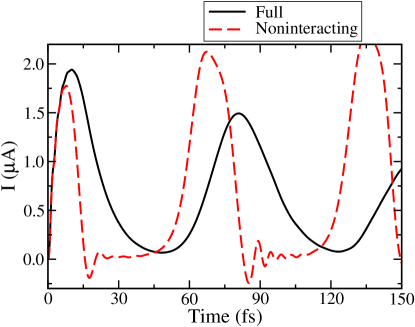
(b)

Figure 1: Comparison of the time-dependent current $I(t)$ between the noninteracting electron approximation and the full ML-MCTDH-SQR simulation where a single vibrational mode is coupled to the bridge state. The frequency is $\omega=500$ cm^-1 and the reorganization energy is $\lambda=2000$ cm^-1. The bias voltage is $V=0.1$V and the initial condition is: (a) an occupied bridge state with the mode’s coordinate shifted to be in equilibrium with it; (b) an empty bridge state with an unshifted mode.

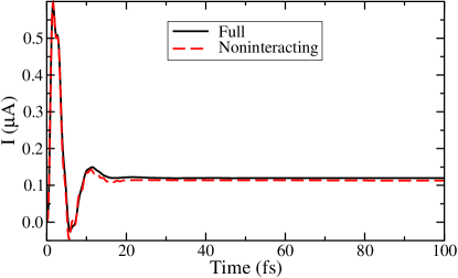
Figure 2: Same as Fig. 1b but for a vibrational bath modeled by an Ohmic spectral density. The characteristic frequency is $\omega_{c}=500$ cm^-1 and the reorganization energy is $\lambda=2000$ cm^-1. The initial condition is specified by an empty bridge state with an unshifted vibrational bath.

(a)

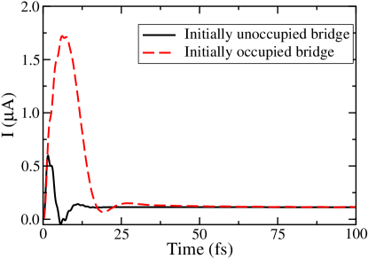
(b)

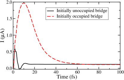
Figure 3: Time-dependent current at different initial conditions: (a) noninteracting electron approximation, (b) full ML-MCTDH-SQR simulation. The characteristic frequency for the vibrational bath is $\omega_{c}=500$ cm^-1 and the reorganization energy is $\lambda=2000$ cm^-1. The bias voltage is $V=0.1$V.

(a)

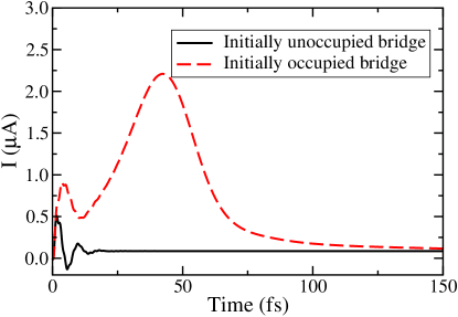
(b)

Figure 4: Time-dependent current at different initial conditions: (a) noninteracting electron approximation, (b) full ML-MCTDH-SQR simulation. The characteristic frequency for the vibrational bath is $\omega_{c}=100$ cm^-1 and the reorganization energy is $\lambda=3000$ cm^-1. The bias voltage is $V=0.1$ V.

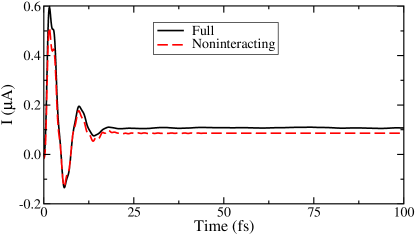
Figure 5: Comparison of the stationary current between the noninteracting electron approximation and the full ML-MCTDH-SQR simulation for the initially unoccupied bridge state and an unshifted vibrational bath. The parameters are the same as in Fig. 4.

(a)

(b)

Figure 6: Time-dependent current at different initial conditions: (a) noninteracting electron approximation, (b) full ML-MCTDH-SQR simulation. The bridge state has the same energy as the Fermi level, $E_{d}-E_{f}=0$. The characteristic frequency for the vibrational bath is $\omega_{c}=500$ cm^-1 and the reorganization energy is $\lambda=2000$ cm^-1. The bias voltage is $V=0.1$ V.

References

- (1) M. Reed, C. Zhou, C. Muller, T. Burgin, and J. Tour, Science 278, 252 (1997).
- (2) C. Joachim, J. Gimzewski, and A. Aviram, Nature (London) 408, 541 (2000).
- (3) A. Nitzan, Annu. Rev. Phys. Chem. 52, 681 (2001).
- (4) A. Nitzan and M. A. Ratner, Science 300, 1384 (2003).
- (5) G. Cuniberti, G. Fagas, and K. Richter, Introducing Molecular Electronics (Springer, Heidelberg, 2005).
- (6) Y. Selzer and D. L. Allara, Annu. Rev. Phys. Chem. 57, 593 (2006).
- (7) L. Venkataraman, J. E. Klare, C. Nuckolls, M. S. Hybertsen, and M. L. Steigerwald, Nature 442, 904 (2006).
- (8) F. Chen, J. Hihath, Z. Huang, X. Li, and N. Tao, Annu. Rev. Phys. Chem. 58, 535 (2007).
- (9) M. Galperin, M. A. Ratner, A. Nitzan, and A. Troisi, Science 319, 1056 (2008).
- (10) J. Cuevas and E. Scheer, Molecular Electronics: An Introduction to Theory and Experiment (World Scientific, Singapore, 2010).
- (11) H. Park, J. Park, A. Lim, E. Anderson, A. Alivisatos, and P. McEuen, Nature (London) 407, 57 (2000).
- (12) X. Cui, A. Primak, X. Zarate, J. Tomfohr, O. Sankey, A. Moore, T. Moore, D. Gust, G. Harris, and S. Lindsay, Science 294, 571 (2001).
- (13) J. Park, A. Pasupathy, J. Goldsmith, C. Chang, Y. Yaish, J. Petta, M. Rinkoski, J. Sethna, H. Abruna, P. McEuen, and D. Ralph, Nature (London) 417, 722 (2002).
- (14) R. Smit, Y. Noat, C. Untiedt, N. Lang, M. van Hemert, and J. van Ruitenbeek, Nature (London) 419, 906 (2002).
- (15) J. Reichert, R. Ochs, D. Beckmann, H. Weber, M. Mayor, and H. von Lohneysen, Phys. Rev. Lett. 88, 176804 (2002).
- (16) B. Xu and N. Tao, Science 301, 1221 (2003).
- (17) X. Qiu, G. Nazin, and W. Ho, Phys. Rev. Lett. 92, 206102 (2004).
- (18) N. Liu, N. Pradhan, and W. Ho, J. Chem. Phys. 120, 11371 (2004).
- (19) M. Elbing, R. Ochs, M. Koentopp, M. Fischer, C. von Hänisch, F. Weigend, F. Evers, H. Weber, and M. Mayor, Proc. Natl. Acad. Sci. USA 102, 8815 (2005).
- (20) N. Ogawa, G. Mikaelian, and W. Ho, Phys. Rev. Lett. 98, 166103 (2007).
- (21) G. Schulze, K. J. Franke, A. Gagliardi, G. Romano, C. S. Lin, A. Da Rosa, T. A. Niehaus, T. Frauenheim, A. Di Carlo, A. Pecchia, and J. Pascual, Phys. Rev. Lett. 100, 136801 (2008).
- (22) F. Pump, R. Temirov, O. Neucheva, S. Soubatch, S. Tautz, M. Rohlfing, and G. Cuniberti, Appl. Phys. A 93, 335 (2008).
- (23) N. P. de Leon, W. Liang, Q. Gu, and H. Park, Nano Lett. 8, 2963 (2008).
- (24) E. A. Osorio, M. Ruben, J. S. Seldenthuis, J. M. Lehn, and H. S. J. van der Zant, Small 6, 174 (2010).
- (25) C. A. Martin, J. M. van Ruitenbeek, and H. S. J. van de Zant, Nanotechnology 21, 265201 (2010).
- (26) W. Liang, M. Shores, M. Bockrath, J. Long, and H. Park, Nature (London) 417, 725 (2002).
- (27) J. Chen, M. Reed, A. Rawlett, and J. Tour, Science 286, 1550 (1999).
- (28) J. Gaudioso, L. J. Lauhon, and W. Ho, Phys. Rev. Lett. 85, 1918 (2000).
- (29) A. Blum, J. Kushmerick, D. Long, C. Patterson, J. Jang, J. Henderson, Y. Yao, J. Tour, R. Shashidhar, and B. Ratna, Nat. Mater. 4, 167 (2005).
- (30) E. Lörtscher, J. W. Ciszek, J. Tour, and H. Riel, Small 2, 973 (2006).
- (31) B.-Y. Choi, S.-J. Kahng, S. Kim, H. Kim, H. Kim, Y. Song, J. Ihm, and Y. Kuk, Phys. Rev. Lett. 96, 156106 (2006).
- (32) S. Ballmann, R. Härtle, P. Coto, M. Elbing, M. Mayor, M. Bryce, M. Thoss, and H. B. Weber, Phys. Rev. Lett. 109, 056801 (2012).
- (33) C. Guedon, H. Valkenier, T. Markussen, K. Thygesen, J. Hummelen, and S. van der Molen, Nat. Nanotechnol. 7, 305 (2012).
- (34) H. Vazquez, R. Skouta, S. Schneebeli, M. Kamenetska, R. Breslow, L. Venkataraman, and M. Hybertsen, Nat. Nanotechnol. 7, 663 (2012).
- (35) R. Landauer, IBM J. Res. Dev. 1, 223 (1951).
- (36) J. Bonca and S. Trugmann, Phys. Rev. Lett. 75, 2566 (1995).
- (37) H. Ness, S. Shevlin, and A. Fisher, Phys. Rev. B 63, 125422 (2001).
- (38) M. Cizek, M. Thoss, and W. Domcke, Phys. Rev. B 70, 125406 (2004).
- (39) M. Cizek, M. Thoss, and W. Domcke, Czech. J. Phys. 55, 189 (2005).
- (40) M. Caspary-Toroker and U. Peskin, J. Chem. Phys. 127, 154706 (2007).
- (41) C. Benesch, M. Cizek, J. Klimes, I. Kondov, M. Thoss, and W. Domcke, J. Phys. Chem. C 112, 9880 (2008).
- (42) N. A. Zimbovskaya and M. M. Kuklja, J. Chem. Phys. 131, 114703 (2009).
- (43) R. Jorn and T. Seidemann, J. Chem. Phys. 131, 244114 (2009).
- (44) K. Flensberg, Phys. Rev. B 68, 205323 (2003).
- (45) A. Mitra, I. Aleiner, and A. J. Millis, Phys. Rev. B 69, 245302 (2004).
- (46) M. Galperin, M. Ratner, and A. Nitzan, Phys. Rev. B 73, 045314 (2006).
- (47) D. A. Ryndyk, M. Hartung, and G. Cuniberti, Phys. Rev. B 73, 045420 (2006).
- (48) T. Frederiksen, M. Paulsson, M. Brandbyge, and A. Jauho, Phys. Rev. B 75, 205413 (2007).
- (49) M. Tahir and A. MacKinnon, Phys. Rev. B 77, 224305 (2008).
- (50) R. Härtle, C. Benesch, and M. Thoss, Phys. Rev. B 77, 205314 (2008).
- (51) J. P. Bergfield and C. A. Stafford, Phys. Rev. B 79, 245125 (2009).
- (52) R. Härtle, C. Benesch, and M. Thoss, Phys. Rev. Lett. 102, 146801 (2009).
- (53) V. May, Phys. Rev. B 66, 245411 (2002).
- (54) J. Lehmann, S. Kohler, V. May, and P. Hänggi, J. Chem. Phys. 121, 2278 (2004).
- (55) J. N. Pedersen and A. Wacker, Phys. Rev. B 72, 195330 (2005).
- (56) U. Harbola, M. Esposito, and S. Mukamel, Phys. Rev. B 74, 235309 (2006).
- (57) A. Zazunov, D. Feinberg, and T. Martin, Phys. Rev. B 73, 115405 (2006).
- (58) L. Siddiqui, A. W. Ghosh, and S. Datta, Phys. Rev. B 76, 085433 (2007).
- (59) C. Timm, Phys. Rev. B 77, 195416 (2008).
- (60) V. May and O. Kühn, Phys. Rev. B 77, 115439 (2008).
- (61) V. May and O. Kühn, Phys. Rev. B 77, 115440 (2008).
- (62) M. Leijnse and M. R. Wegewijs, Phys. Rev. B 78, 235424 (2008).
- (63) M. Esposito and M. Galperin, Phys. Rev. B 79, 205303 (2009).
- (64) R. Härtle and M. Thoss, Phys. Rev. B 83, 115414 (2011).
- (65) L. Mühlbacher and E. Rabani, Phys. Rev. Lett. 100, 176403 (2008).
- (66) S. Weiss, J. Eckel, M. Thorwart, and R. Egger, Phys. Rev. B 77, 195316 (2008).
- (67) D. Segal, A.J.Millis, and D. Reichman, Phys. Rev. B 82, 205323 (2010).
- (68) P. Werner, T. Oka, and A. J. Millis, Phys. Rev. B 79, 035320 (2009).
- (69) M. Schiro and M. Fabrizio, Phys. Rev. B 79, 153302 (2009).
- (70) F. B. Anders, Phys. Rev. Lett. 101, 066804 (2008).
- (71) H. Wang and M. Thoss, J. Chem. Phys. 131, 024114 (2009).
- (72) H. Wang, I. Pshenichnyuk, R. Härtle, and M. Thoss, J. Chem. Phys. 135, 244506 (2011).
- (73) H. Wang and M. Thoss, J. Chem. Phys. 138, 134704 (2013).
- (74) H. Wang and M. Thoss, J. Phys. Chem. A 117, 7431 (2013).
- (75) E. Y. Wilner, H. Wang, G. Cohen, M. Thoss, and E. Rabani, Phys. Rev. B 88, 045137 (2013).
- (76) B. Stipe, M. Rezai, and W. Ho, Science 280, 1732 (1998).
- (77) L. H. Yu, Z. K. Keane, J. W. Ciszek, L. Cheng, M. P. Stewart, J. M. Tour, and D. Natelson, Phys. Rev. Lett. 93, 266802 (2004).
- (78) J. Kushmerick, J. Lazorcik, C. Patterson, R. Shashidhar, D. S. Seferos, and G. C. Bazan, Nano Lett. 4, 639 (2004).
- (79) A. Pasupathy, J. Park, C. Chang, A. Soldatov, S. Lebedkin, R. Bialczak, J. Grose, L. Donev, J. Sethna, D. Ralph, and P. McEuen, Nano Lett. 5, 203 (2005).
- (80) S. Sapmaz, P. Jarillo-Herrero, Y. M. Blanter, C. Dekker, and H. S. van der Zant, Phys. Rev. Lett. 96, 026801 (2006).
- (81) W. H. A. Thijssen, D. Djukic, A. F. Otte, R. H. Bremmer, and J. M. van Ruitenbeek, Phys. Rev. Lett. 97, 226806 (2006).
- (82) J. Parks, A. Champagne, G. Hutchison, S. Flores-Torres, H. Abruna, and D. Ralph, Phys. Rev. Lett. 99, 026601 (2007).
- (83) T. Böhler, A. Edtbauer, and E. Scheer, Phys. Rev. B 76, 125432 (2007).
- (84) Z. Huang, B. Xu, Y. Chen, M. D. Ventra, and N. Tao, Nano Lett. 6, 1240 (2006).
- (85) D. R. Ward, N. J. Halas, J. W. Ciszek, J. M. Tour, Y. Wu, P. Nordlander, and D. Natelson, Nano Lett. 8, 919 (2008).
- (86) Z. Ioffe, T. Shamai, A. Ophir, G. Noy, I. Yutsis, K. Kfir, O. Cheshnovsky, and Y. Selzer, Nature Nanotech. 3, 727 (2008).
- (87) A. K. Hüttel, B. Witkamp, M. Leijnse, M. R. Wegewijs, and H. S. J. van der Zant, Phys. Rev. Lett. 102, 225501 (2009).
- (88) S. Ballmann, W. Hieringer, D. Secker, Q. Zheng, J. A. Gladysz, A. Görling, and H. B. Weber, Chem. Phys. Chem. 11, 2256 (2010).
- (89) D. Secker, S. Wagner, S. Ballmann, R. Härtle, M. Thoss, and H. B. Weber, Phys. Rev. Lett. 106, 136807 (2011).
- (90) S. Ballmann, W. Hieringer, R. Härtle, P. Coto, M. Bryce, A. Görling, M. Thoss, and H. B. Weber, Phys. Status Solidi B 250, 2452 (2013).
- (91) Y. Zhang, C. Y. Yam, and G. Chen, J. Chem. Phys. 138, 164121 (2013).
- (92) C. Verdozzi, G. Stefanucci, and C. Almbladh, Phys. Rev. Lett. 97, 046603 (2006).
- (93) A. J. Leggett, S. Chakravarty, A. T. Dorsey, M. P. A. Fisher, A. Garg, and W. Zwerger, Rev. Mod. Phys. 59(1), 1 (1987).
- (94) U. Weiss, Quantum Dissipative Systems (World Scientific, Singapore, 1993).
- (95) H. Wang and M. Thoss, J. Chem. Phys. 119, 1289 (2003).
- (96) K. F. Albrecht, H. Wang, L. Mühlbacher, M. Thoss, and A. Komnik, Phys. Rev. B 86, 081412 (2012).
- (97) H. Wang, J. Phys. Chem. A 119, 7951 (2015).
- (98) H.-D. Meyer, U. Manthe, and L. Cederbaum, Chem. Phys. Lett. 165, 73 (1990).
- (99) H.-D. Meyer, F. Gatti, and G. Worth, Multidimensional Quantum Dynamics: MCTDH Theory and Applications (Whiley-VCH, Weinheim, 2009).
- (100) M. Thoss and H. Wang, Chem. Phys. 322, 210 (2006).
- (101) H. Wang and M. Thoss, J. Chem. Phys. 124, 034114 (2006).
- (102) I. Kondov, H. Wang, and M. Thoss, J. Phys. Chem. A 110, 1364 (2006).
- (103) H. Wang and M. Thoss, J. Phys. Chem. A 111, 10369 (2007).
- (104) I. Kondov, M. Cizek, C. Benesch, H. Wang, and M. Thoss, J. Phys. Chem. C 111(32), 11970 (2007).
- (105) M. Thoss, I. Kondov, and H. Wang, Phys. Rev. B 76, 153313 (2007).
- (106) I. R. Craig, M. Thoss, and H. Wang, J. Chem. Phys. 127, 144503 (2007).
- (107) H. Wang and M. Thoss, Chem. Phys. 347, 139 (2008).
- (108) H. Wang and M. Thoss, New J. Phys. 10, 115005 (2008).
- (109) D. Egorova, M. F. Gelin, M. Thoss, H. Wang, and W. Domcke, J. Chem. Phys. 129, 214303 (2008).
- (110) K. A. Velizhanin, H. Wang, and M. Thoss, Chem. Phys. Lett. 460, 325 (2008).
- (111) K. A. Velizhanin and H. Wang, J. Chem. Phys. 131, 094109 (2009).
- (112) H. Wang and M. Thoss, Chem. Phys. 370, 78 (2010).
- (113) Y. Zhou, J. Shao, and H. Wang, Mol. Phys. 110, 581 (2012).
- (114) H. Wang and S. Shao, J. Chem. Phys. 137, 22A504 (2012).
- (115) U. Manthe, J. Chem. Phys. 128, 164116 (2008).
- (116) U. Manthe, J. Chem. Phys. 130, 054109 (2009).
- (117) M. Thoss, I. Kondov, and H. Wang, Chem. Phys. 304, 169 (2004).
- (118) J. Li, H. Wang, and M. Thoss, J. Phys.: Condens. Matter 27, 134202 (2015).
- (119) H. Ness and A. Fisher, Proc. Natl. Acad. Sci. USA 102, 8826 (2005).
- (120) C. Benesch, M. Cizek, M. Thoss, and W. Domcke, Chem. Phys. Lett. 430, 355 (2006).
(a)
(b)
(a)
(b)
(a)
(b)
(a)
(b)