Universal Quantum Emulator

Abstract

We propose a quantum algorithm that emulates the action of an unknown unitary transformation on a given input state, using multiple copies of some unknown sample input states of the unitary and their corresponding output states. The algorithm does not assume any prior information about the unitary to be emulated, or the sample input states. To emulate the action of the unknown unitary, the new input state is coupled to the given sample input-output pairs in a coherent fashion. Remarkably, the runtime of the algorithm is logarithmic in $D$, the dimension of the Hilbert space, and increases polynomially with $d$, the dimension of the subspace spanned by the sample input states. Furthermore, the sample complexity of the algorithm, i.e. the total number of copies of the sample input-output pairs needed to run the algorithm, is independent of $D$, and polynomial in $d$. In contrast, the runtime and the sample complexity of incoherent methods, i.e. methods that use tomography, are both linear in $D$. The algorithm is blind, in the sense that at the end it does not learn anything about the given samples, or the emulated unitary. This algorithm can be used as a subroutine in other algorithms, such as quantum phase estimation.

I Introduction

A universal quantum simulator is a machine that can be programmed to mimic the dynamics of other quantum systems S. Lloyd (1996). The time evolution of the simulator obeys the same equations of motion as the evolution of the simulated system. A universal quantum emulator, on the other hand, is a machine that mimics the input-output relation of another system, by looking to the output of that system on some sample input states. Unlike a simulator, an emulator does not need to obey the same dynamical equations as of the emulated system.

In this Letter we introduce a quantum algorithm that emulates the action of an unknown unitary transformation on new given input states. The algorithm couples the new input state to multiple copies of some unknown sample input-output pairs, that is copies of some input states of the unitary as well as copies of the corresponding output states. We do not assume any prior information about the unitary to be emulated, or the given sample input states. The algorithm emulates the action of the unitary on any given state in the subspace spanned by the previously given input states, which could be much smaller than the system Hilbert space. Indeed, we are interested in the cases where $d$, the dimension of this subspace is constant or, at most, polylogarithmic in $D$, the dimension of the system Hilbert space.

Obviously, having multiple copies of sample input-output pairs we can perform measurements on them, and using state tomography find an approximate classical description of these states in a standard basis. This, in turn, yields the classical description of the unknown unitary transformation, which then can be used to simulate its action on the new given states. This approach, however, is highly inefficient and impractical: First of all, state tomography in a large Hilbert space is a hard task and requires lots of copies of the sample states. Second, even if we find an approximate classical description of the unitary transformation, or if we are given its exact description, in general we cannot implement this transformation on a new given state efficiently.

More precisely, the approaches based on tomography run in time $\Omega(D)$ and need $\Omega(D)$ copies of state, where $D$ is the dimension of the system Hilbert space. In contrast, the runtime of the algorithm proposed in this work is $\mathcal{O}(\log D)$ and polynomial in $d$, and its sample complexity, i.e. the total number of copies of the sample input-output pairs that are needed to run the algorithm, is independent of $D$ and polynomial in $d$. Therefore, our algorithm is not only exponentially faster than the approaches based on tomography, its sample complexity is also dramatically lower.

It is interesting to compare this result with the scenario studied in Bisio et al. (2010), where one wants to learn an unknown unitary $U$ by applying it for a finite number of times to some quantum states, so that later, when we do not have access to $U$, we can reproduce its effect on a new input state. It turns out that the strategy that maximizes the average fidelity, where the average is taken over all states in the Hilbert space, is an incoherent measure-and-rotate strategy, i.e. a method that uses tomography Bisio et al. (2010). In contrast to this result, our work shows that under the practical assumption that the action of the unitary should be emulated in a low-dimensional subspace, and not the entire Hilbert space, the coherent methods are much more powerful than the incoherent ones.

This algorithm is blind, in the sense that at the end it does not learn anything about the given samples, or the emulated unitary. Although the algorithm uses a randomized technique, it always generates an output with high fidelity with the desired output state. Therefore, it can be used as a subroutine in larger algorithms, such as quantum phase estimation. Another possible application of this algorithm is to use it to cancel the effect of an unknown unitary channel, without doing process tomography and finding the description of the unitary. Furthermore, the algorithm could be useful in the cases where we can prepare the input and the corresponding outputs of a unitary transformation efficiently, but we do not know how to implement the unitary itself.

II Preliminaries

We first present the algorithm for the special case of pure sample states, and later explain how it can be generalized to the case of mixed states as well.

Let $S_{\text{in}}=\{|\phi^{\text{in}}_{k}\rangle\langle\phi_{k}^{\text{in}}|:k=1,\cdots,K\}$ be a set of sample input states of the unitary $U$ and $S_{\text{out}}=\{|\phi^{\text{out}}_{k}\rangle\langle\phi_{k}^{\text{out}}|=U|\phi^{\text{in}}_{k}\rangle\langle\phi_{k}^{\text{in}}|U^{\dagger}:k=1,\cdots,K\}$ be the corresponding outputs. Let $\mathcal{H}_{\text{in}}$ and $\mathcal{H}_{\text{out}}$ be the subspaces spanned by $\{|\phi^{\text{in}}_{k}\rangle:k=1,\cdots,K\}$ and $\{|\phi^{\text{out}}_{k}\rangle:k=1,\cdots,K\}$ respectively, and $d$ be the dimension of these subspaces. We assume the set of input samples $S_{\text{in}}$ contains sufficient number of different states to uniquely determine the action of $U$ on the subspace $\mathcal{H}_{\text{in}}$ (up to a global phase). It can be easily shown that having the classical description of the input and output states in $S_{\text{in}}$ and $S_{\text{out}}$ we can uniquely determine the action of $U$ on any input state $|\psi\rangle\in\mathcal{H}_{\text{in}}$ (up to a global phase), if and only if the matrix algebra generated by $S_{\text{in}}$, that is the set of polynomials in the elements of $S_{\text{in}}$, is the full matrix algebra on $\mathcal{H}_{\text{in}}$, i.e. contains all operators with supports contained in $\mathcal{H}_{\text{in}}$. Therefore, in the following we naturally assume this assumption is satisfied. Furthermore, we assume $K$ the number of different sample input states in $S_{\text{in}}$ is $\text{poly}(d)$.

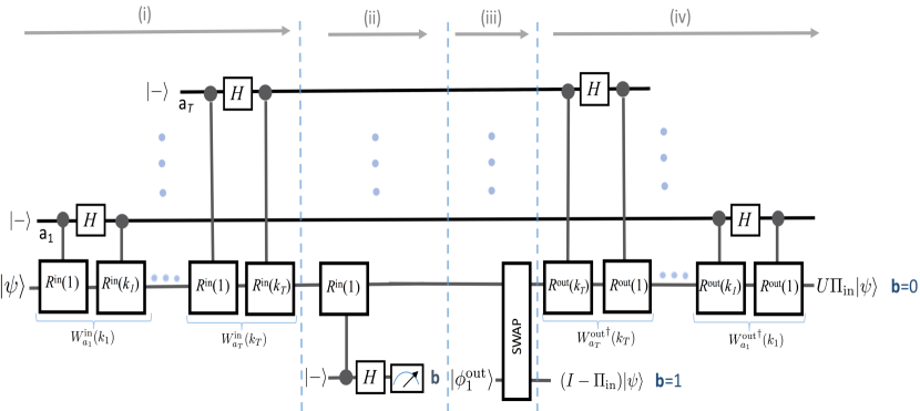
Figure 1: The quantum circuit for emulating unitary transformation $U$ for the special case of pure input-output sample pairs. Here $k_{1},\cdots,k_{T}$ are $T=\text{poly}(d)$ integers chosen uniformly at random from integers $1,\cdots,K$. We use the given copies of sample states in $S_{\text{in}}$ and $S_{\text{out}}$ to simulate the controlled-reflections $R_{a}^{\text{in}}(k)$ and $R_{a}^{\text{out}}(k)$, respectively.

To implement the algorithm, we need multiple copies of each sample state in $S_{\text{in}}$ and $S_{\text{out}}$. Interestingly, at the end of the algorithm most of these states remain almost unaffected. Indeed, the main use of the given copies of sample states is to simulate controlled-reflections about these states.

Let $R^{\text{in}}(k)=e^{i\pi|\phi^{\text{in}}_{k}\rangle\langle\phi^{\text{in}}_{k}|}$ and $R^{\text{out}}(k)=e^{i\pi|\phi^{\text{out}}_{k}\rangle\langle\phi^{\text{out}}_{k}|}$ be the reflections about the input and output states $|\phi^{\text{in}}_{k}\rangle$ and $|\phi^{\text{out}}_{k}\rangle$, respectively. In the proposed algorithm we need to implement the controlled-reflections $R_{a}^{\text{in}}(k)$ and $R_{a}^{\text{out}}(k)$, defined as

$$R_{a}(k) =|0\rangle\langle 0|_{a}\otimes I+|1\rangle\langle 1|_{a}\otimes e^{i\pi|\phi_{k}\rangle\langle\phi_{k}|}\ ,$$ (1)

where $a$ is the label for the control qubit, and $I$ is the identity operator on the main system. Note that we have suppressed the superscripts in and out in both sides.

Using the given copies of the sample states, we can efficiently simulate these controlled-reflections via the density matrix exponentiation technique of Lloyd et al. (2014). Based on this technique, in the Supplementary Material we present a new simple quantum circuit that uses $n$ copies of an unknown state $\sigma$ to simulate the unitary $e^{-it\sigma}$, or its controlled version $|0\rangle\langle 0|\otimes I+|1\rangle\langle 1|\otimes e^{-it\sigma}$, for any real $t$, with error $\epsilon=\mathcal{O}((t^{2}+1)/n)$, and in time $\mathcal{O}(n\log(n)\times\log(D))$, where $D$ is the dimension of the Hilbert space (See Appendix C). This circuit only uses single qubit gates and controlled-Fredkin gates, i.e. the controlled-controlled-SWAP gates Nielsen and Chuang (2000). In the simplest case where the system is a qubit $(D=2)$, this circuit is basically simulating the Heisenberg interaction between the system and each given copy of state $\sigma$.

Therefore, in the following, where we present the algorithm, we assume all the controlled-reflections $\{R_{a}(k):1\leq k\leq K\}$ can be efficiently implemented.

To simplify the presentation, we use the notation $W_{a}(k)\equiv R_{a}(k)H_{a}R_{a}(1)$, where again we have suppressed in and out superscripts in both sides. Here $H_{a}$ denotes the Hadamard gate $H$ acting on qubit $a$, where $H|0\rangle=|+\rangle$ and $H|1\rangle=|-\rangle$, and $|\pm\rangle=(|0\rangle\pm|1\rangle)/\sqrt{2}$. The algorithm also uses a SWAP gate defined by $\text{SWAP}|\nu\rangle|\mu\rangle=|\mu\rangle|\nu\rangle$, for any pair of states $|\mu\rangle$ and $|\nu\rangle$.

III The algorithm (Special case)

In this section we present and analyze the algorithm for the universal quantum emulator, in the special case where all the sample input-output pairs are pure states. Later, we present several generalizations of this algorithm, including to the case where the given samples contain mixed states.

Fig.(1) exhibits the quantum circuit that emulates the action of an unknown unitary transformation $U$ on any given state $|\psi\rangle$ in the input subspace $\mathcal{H}_{\text{in}}$. For a general input state, which is not restricted to this subspace, this circuit first projects the state to this subspace, and if successful, then applies the unitary $U$ to it.

In this algorithm $(k_{1},\cdots,k_{T})$ are $T$ integers chosen uniformly at random from integers $1,\cdots,K$, where $T$ is a constant that determines the precision of emulation, and we choose it to be polynomial in $d$, and independent of $D$. Furthermore, state $|\phi_{1}^{\text{in}}\rangle$ (and $|\phi_{1}^{\text{out}}\rangle$) is one of the sample input states (and its corresponding output) which is chosen randomly at the beginning of the algorithm, and is fixed during the algorithm. In steps (i) and (iv) of the algorithm we implement, respectively, the unitaries $W_{a_{i}}^{\text{in}}(k_{i})$ and ${W_{a_{i}}^{\text{out}}}^{\dagger}(k_{i})$ on the system and qubit $a_{i}$, for $i=1,\cdots,T$. As we explained before, all the conditional reflections $R^{\text{in}}_{a}(k)$ and $R^{\text{out}}_{a}(k)$ can be efficiently simulated using the given copies of states $|\phi_{k}^{\text{in}}\rangle$ and $|\phi_{k}^{\text{out}}\rangle$.

In step (ii) of the algorithm we perform a qubit measurement in the computational basis $\{|0\rangle,|1\rangle\}$. Then, after the measurement with probability $1-\langle\psi|\Pi_{\text{in}}|\psi\rangle$ we get outcome $b=1$, in which case we project the system to a state close to $(I-\Pi_{\text{in}})|\psi\rangle/\sqrt{1-\langle\psi|\Pi_{\text{in}}|\psi\rangle}$, where $\Pi_{\text{in}}$ is the projector to the subspace $\mathcal{H}_{\text{in}}$. On the other hand, with probability $\langle\psi|\Pi_{\text{in}}|\psi\rangle$ we get the outcome $b=0$, in which case the final state of circuit is close to $U\Pi_{\text{in}}|\psi\rangle/\sqrt{\langle\psi|\Pi_{\text{in}}|\psi\rangle}$. In this case the algorithm consumes a copy of state $|\phi_{1}^{\text{out}}\rangle$, and returns a copy of state $|\phi_{1}^{\text{in}}\rangle$.

Note that, although the algorithm uses random integers $(k_{1},\cdots,k_{T})$, for sufficiently large $T$ it always transforms the input state $|\psi\rangle\in\mathcal{H}_{\text{in}}$ to a state with high fidelity with the desired output state $U|\psi\rangle$.

III.1 How it works

To simplify the following discussion, we first assume the initial state $|\psi\rangle$ is in the input subspace $\mathcal{H}_{\text{in}}$, and then we consider the general case.

To understand step (i) of the algorithm, we first focus on the reduced state of the system. From this point of view, during step (i) we are trying to erase the state of system and push it into $|\phi_{1}^{\text{in}}\rangle$, a state which is chosen randomly from the sample input set $S_{\text{in}}$. This erasing is done by repetitive measuring and conditional mixing.

Consider the first round of step (i), where we have randomly chosen integer $k_{1}$ in $1,\cdots,K$, and apply the unitary $W(k_{1})=R_{a_{1}}(k_{1})H_{a_{1}}R_{a_{1}}(1)$ to the system and qubit $a_{1}$ initially prepared in state $|-\rangle$. The effect of this transformation on the reduced state of system can be interpreted in the following way: we perform a measurement in $\{P=|\phi_{1}^{\text{in}}\rangle\langle\phi_{1}^{\text{in}}|,P^{\perp}=I-P\}$ basis, and if the system is found in state $|\phi_{1}^{\text{in}}\rangle$, we leave it unchanged; otherwise, we apply the random reflection $R^{\text{in}}(k_{1})$ to it. Tracing over qubit $a_{1}$, and averaging over the values of $k_{1}$, we find that the overall effect of this transformation on the reduced state of system can be described by the quantum channel $\mathcal{W}(\rho)=P\rho P+\mathcal{D}(P^{\perp}\rho P^{\perp})$, where

$$\mathcal{D}(\rho)=\frac{1}{K}\sum^{K}_{k=1}R^{\text{in}}(k)\ \rho\ R^{\text{in}}(k)\ .$$ (2)

In step (i) we repeat the above procedure for $T$ times with $T$ different ancillary qubits and random integers. Using the facts that (1) ancillary qubits are initially uncorrelated with each other, and (2) different random integers $k_{1},\cdots,k_{T}$ are statistically independent of each other, we find that at the end of step (i) the average reduced state of system is described by state $\mathcal{W}^{T}(|\psi\rangle\langle\psi|)$.

Next, recall the assumption that the input set $S_{\text{in}}$ generates the full matrix algebra in $\mathcal{H}_{\text{in}}$, an assumption which is crucial for being able to uniquely determine the action of $U$ on $\mathcal{H}_{\text{in}}$. Interestingly, this assumption now translates to the fact that channels $\mathcal{D}$ and $\mathcal{W}$ have unique fixed point states with support contained in $\mathcal{H}_{\text{in}}$, namely the totally mixed state in $\mathcal{H}_{\text{in}}$, and $|\phi_{1}^{\text{in}}\rangle\langle\phi_{1}^{\text{in}}|$ respectively. Furthermore, since the reflections $R^{\text{in}}(k)$ are block diagonal with respect to the input subspace $\mathcal{H}_{\text{in}}$, channels $\mathcal{D}$ and $\mathcal{W}$ map any initial state inside $\mathcal{H}_{\text{in}}$ to a state with support contained in this subspace. It follows that for any initial state $|\psi\rangle\in\mathcal{H}_{\text{in}}$, at the end of step (i) with probability almost one the system should be in state $|\phi_{1}^{\text{in}}\rangle$. More precisely, the probability of finding the system in a state orthogonal to $|\phi_{1}^{\text{in}}\rangle$ is exponentially small in $T$.

To summarize, in step (i) we erase the initial state of system and push it into state $|\phi_{1}^{\text{in}}\rangle$. The fact that we have enough resources to uniquely determine the action of unitary $U$ on any state in the input subspace $\mathcal{H}_{\text{in}}$, translates to the fact that any state in this subspace can be erased in a coherent unitary fashion.

But quantum information is conserved during a unitary evolution. This means that all the information about state $|\psi\rangle$ should now be encoded in the ancillary qubits $\textbf{a}=a_{1}\cdots a_{T}$. Furthermore, since we start with a global pure state, and since at the end of step (i) the reduced state of system is close to a pure state, we find that the joint reduced state of ancillary qubits a should also be close to a pure state, denoted by $|\Psi(\textbf{k})\rangle_{\textbf{a}}$. Note that in addition to state $|\psi\rangle$, state $|\Psi(\textbf{k})\rangle_{\textbf{a}}$ also depends on the sample set $S_{\text{in}}$, and the random integers $\textbf{k}\equiv(k_{1},\cdots,k_{T})$. We conclude that at the end of step (i) with high probability the system and ancillary qubits a are in the product state

$$\left[{W_{a_{T}}^{\text{in}}}({k_{T}})\cdots{W_{a_{1}}^{\text{in}}}({k_{1}})\right]|\psi\rangle|-\rangle^{\otimes T}\approx|\phi_{1}^{\text{in}}\rangle|\Psi(\bf{k})\rangle_{\textbf{a}}\ .$$ (3)

Next, in step (ii) we basically perform a measurement on the system in $\{P=|\phi_{1}^{\text{in}}\rangle\langle\phi_{1}^{\text{in}}|,P^{\perp}=I-P\}$ basis. At this point we know that for any initial state $|\psi\rangle\in\mathcal{H}_{\text{in}}$ with probability almost one the system should be in state $|\phi_{1}^{\text{in}}\rangle$, in which case the measurement projects the ancillary qubit to state $|0\rangle$. On the other hand, if we project the qubit to state $|1\rangle$ it means the erasing has not been successful.

Finally, assuming $|\psi\rangle\in\mathcal{H}_{\text{in}}$, we find that applying steps (iii) and (iv) maps the system to state $U|\psi\rangle$. This can be seen by multiplying both sides of Eq.(3) in unitary $U$, and using the facts that $U|\phi_{1}^{\text{in}}\rangle=|\phi_{1}^{\text{out}}\rangle$, and $(U\otimes I_{a})W^{\text{in}}_{a}(k)(U^{\dagger}\otimes I_{a})=W^{\text{out}}_{a}(k)$. This implies

$$\left[{W_{a_{1}}^{\text{out}}}^{\dagger}({k_{1}})\cdots{W_{a_{T}}^{\text{out}}}^{\dagger}({k_{T}})\right]|\phi_{1}^{\text{out}}\rangle|\Psi(\textbf{k})\rangle_{\textbf{a}}\approx U|\psi\rangle|-\rangle^{\otimes T}\ .$$ (4)

Eq.(4) means that, after step (ii) by preparing the system in the output sample state $|\phi_{1}^{\text{out}}\rangle$, which is given to us, and running all the operations in step (i) backward, with unitaries $R_{a}^{\text{in}}(k)$ replaced by $R_{a}^{\text{out}}(k)$, we get state $U|\psi\rangle$ at the end.

Using the fact that all unitaries $W_{a}(k)=R_{a}(k)H_{a}R_{a}(1)$ act trivially on the subspace orthogonal to $\mathcal{H}_{\text{in}}$, it can be easily seen that for a general input $|\psi\rangle$, which is not contained in $\mathcal{H}_{\text{in}}$, the algorithm first performs a projective measurement that projects the input state to the subspace $\mathcal{H}_{\text{in}}$, or the orthogonal subspace. Then, if the system is found to be in $\mathcal{H}_{\text{in}}$, which corresponds to outcome $b=0$ in the measurement in step (ii), it applies the unitary $U$ to the component of state in this subspace.

In the Supplementary Material we prove the following quantitative version of the above argument: Suppose we implement the quantum circuit presented in Fig. 1, using perfect controlled-reflections $R_{a}(k)$. Let $\mathcal{E}_{U}$ be the quantum channel that describes the overall effect of the circuit on the system, in the case where we do not postselect based on the outcome of measurement in step (ii), which means we do not care if erasing has been successful or not. Then, for an arbitrary input state $\rho$, the (Uhlmann) fidelity Uhlmann (1976); Jozsa (1994) of $\mathcal{E}_{U}(\rho)$ and the desired state $U\rho U^{\dagger}$ satisfies

$$\text{F}(\mathcal{E}_{U}(\rho),U\rho U^{\dagger})\geq p_{\text{erase}}(\rho)=\langle\phi^{\text{in}}_{1}|\mathcal{W}^{T}(\rho)|\phi^{\text{in}}_{1}\rangle\ ,$$ (5)

where $p_{\text{erase}}(\rho)$ is the probability that we have successfully erased the state of system (and pushed it into state $|\phi^{\text{in}}_{1}\rangle$), which corresponds to outcome $0$ in the measurement (See Appendix A). On the other hand, if we postselect to the cases where the erasing has been successful, then for pure input state $\rho$, the fidelity between the output of the algorithm and the desired state $U\rho U^{\dagger}$ is lower bounded by $\sqrt{p_{\text{erase}}(\rho)}$.

Interestingly, as we show in the Supplementary Material, Eq.(5) holds in a much more general setting: suppose we run the above algorithm with any other choice of unitaries $W_{a}^{\text{in}}(\lambda)$ and $W^{\text{out}}_{a}(\lambda)=(U\otimes I_{a})W^{\text{in}}_{a}(\lambda)(U^{\dagger}\otimes I_{a})$ that couple the system to a qubit $a$, where $\lambda$ is a random parameter chosen according to a probability distribution $p(\lambda)$. Then, Eq.(5) still holds for the channel $\mathcal{W}(\tau)=\sum_{\lambda}p(\lambda)\textrm{Tr}_{a}\big{(}W_{a}^{\text{in}}(\lambda)[\tau\otimes|-\rangle\langle-|_{a}]{W_{a}^{\text{in}}}^{\dagger}(\lambda)\big{)}$. In the Supplementary Material we use this generalization to extend the algorithm to the case where the samples contain mixed states.

Eq.(5) best captures the working principle behind this algorithm, which can be called emulating via coherent erasing. Note that using this equation we can determine for which input states, the emulation works well: if we have the required resources to coherently erase state $\rho$ and bring the system to a pure state which we know how transforms under unitary $U$, then we can emulate the action of unitary $U$ on $\rho$.

III.2 Coordinates of the input state relative to the samples

As we saw before, at the end of step (i) all the information about the input state $|\psi\rangle$ is encoded in the ancillary qubits. Finding the explicit form of this encoded version of state clarifies an interesting interpretation of this algorithm: step (i) of the algorithm finds the coordinates of the input state $|\psi\rangle$ relative to the frame defined by the input samples $|\phi^{\text{in}}_{k_{1}}\rangle,\cdots,|\phi^{\text{in}}_{k_{T}}\rangle$. Then, step (iv) reconstructs the state with exactly the same coordinates relative to the frame defined by the output samples $|\phi^{\text{out}}_{k_{1}}\rangle,\cdots,|\phi^{\text{out}}_{k_{T}}\rangle$.

Let $|t\rangle_{\textbf{a}}=|1\rangle^{\otimes t}\otimes|0\rangle^{\otimes(T-t)}$ be the state of qubits $a_{1}\cdots a_{T}$, in which $a_{t+1}\cdots a_{T}$ are all in state $|0\rangle$, and the rest of qubits are in state $|1\rangle$. Then, at the end of step (i) the joint state of the system and $\textbf{a}=a_{1}\cdots a_{T}$ is given by

$$|\phi^{\text{in}}_{1}\rangle\sum_{t=0}^{T-1}\langle\phi^{\text{in}}_{1}|\psi(t,\textbf{k})\rangle\ |t\rangle_{\textbf{a}}+|\psi(T,\textbf{k})\rangle|T\rangle_{\textbf{a}}\ ,$$ (6)

where the (unnormalized) vectors $|\psi(t,\textbf{k})\rangle$ are defined via the recursive relation

$$|\psi(t+1,\textbf{k})\rangle=R^{\text{in}}(k_{t+1})P^{\perp}|\psi(t,\textbf{k})\rangle\ ,$$ (7)

and $|\psi(0,\textbf{k})\rangle=|\psi\rangle$. The argument in the previous section implies that for initial state $|\psi\rangle\in\mathcal{H}_{\text{in}}$, the typical norm of $|\psi(t,\textbf{k})\rangle$ is exponentially small in $t$, and hence for sufficiently large $T$ the last term in Eq.(6) is negligible. It follows that this expansion indeed describes a general recursive method for specifying any vector $|\psi\rangle\in\mathcal{H}_{\text{in}}$ in terms of the scalars $\{\langle\phi^{\text{in}}_{1}|\psi(t,\textbf{k})\rangle:t=0,\cdots,T-1\}$. These scalars only depend on the relation between $|\psi\rangle$ and states $|\phi^{\text{in}}_{k_{1}}\rangle,\cdots,|\phi^{\text{in}}_{k_{T}}\rangle$, i.e. applying the same unitary transformation on $|\psi\rangle$ and these states leaves them invariant. We can interpret these scalars as the coordinates of vector $|\psi\rangle$ relative to the frame defined by states $|\phi^{\text{in}}_{k_{1}}\rangle,\cdots,|\phi^{\text{in}}_{k_{T}}\rangle$. Then, in this language, the step (i) of the algorithm is a circuit for finding the coordinates of the given state $|\psi\rangle$ relative to the input frame $|\phi^{\text{in}}_{k_{1}}\rangle,\cdots,|\phi^{\text{in}}_{k_{T}}\rangle$. Note that because of the no-cloning theorem Wootters and Zurek (1982), in order to find the coordinates of a quantum state in a reversible fashion and encode it in the ancillary qubits, we need to erase the state of system.

Therefore, the step (i) of this algorithm provides an efficient reversible method for finding the coordinates of a given state with respect to a general frame, using multiple copies of states corresponding to that frame . This method can be useful for other applications, where instead of implementing operations on the system directly, we first find the coordinates of state of system with respect to other quantum states, implement an operation on the coordinates, and then transform the state back to the physical space.

III.3 Runtime and error analysis

It follows from Eq.(5) that if we run the circuit in Fig.(1) with ideal controlled-reflections, then for any initial state $|\psi\rangle\in\mathcal{H}_{\text{in}}$, the trace distance between the output of the circuit and the desired state $U|\psi\rangle$ is less than or equal to $\epsilon$, provided that we choose

$$T\geq\frac{d\times\log(8d\epsilon^{-2})}{1-|\lambda_{\mathcal{D}}|}\ ,$$ (8)

where $\lambda_{\mathcal{D}}$ is the eigenvalue of channel $\mathcal{D}$ with the second largest magnitude (See Appendix B). Therefore, as one expects from the discussion in the previous section, the runtime is mainly determined by the the mixing time of the random unitary channel $\mathcal{D}$, or equivalently, its spectral gap $1-|\lambda_{\mathcal{D}}|$.

It turns out that in the actual algorithm for the universal quantum emulator, where we need to simulate the controlled-reflections using the given copies of sample states, the dominant source of error is due to the imperfections in these simulations. In the Supplementary Material we show that for initial state $|\psi\rangle\in\mathcal{H}_{\text{in}}$, the transformation $|\psi\rangle\rightarrow U|\psi\rangle$ can be implemented with error $\epsilon>0$ in the trace distance, using

$$N_{\text{tot}}=\tilde{\mathcal{O}}\big{(}\frac{d^{2}\times\epsilon^{-1}}{(1-|\lambda_{\mathcal{D}}|)^{2}}\big{)}\$$ (9)

total copies of sample states, and in time $t_{\text{tot}}=\tilde{\mathcal{O}}(N_{\text{tot}}\times\log D)$, where $\tilde{\mathcal{O}}$ suppresses more slowly-growing terms (See Appendix B.2). Note that the only place where $D$, the dimension of Hilbert space, shows up in the analysis is in the simulation of the controlled-reflections.

III.4 Optimality

In contrast with the approaches based on tomography, whose runtime and sample complexity both scales (at least) linearly with $D$, the runtime $t_{\text{tot}}$ of the above algorithm is only logarithmic in $D$, whilst its sample complexity $N_{\text{tot}}$ is independent of $D$.

In general, the lowest achievable runtime is lower bounded by $\Omega(\log^{\gamma}D)$, where $\gamma$ is a constant of order one depending on the circuit architecture. This is because, in general, the state of each qubit in the desired output state $U|\psi\rangle$ depends non-trivially on the state of all other qubits in state $|\psi\rangle$, as well as the state of all qubits in the sample states. This means that the runtime of the algorithm is bounded by the minimum time required for information about one qubit in the system to propagate to all other qubits. Since the quantum circuit is formed from local unitary gates each acting on few qubits, this time grows with $\log D$, the number of qubits. For instance, in the case where qubits are all on a line and interact only with their nearest neighbors, this time is of the order $\log D$.

Furthermore, it can be easily seen that the lowest achievable runtime scales, at least, linearly with $d$, the dimension of the input subspace. Indeed, just to check if the given state is inside the input subspace spanned by the sample states, one needs to interact with at least $d$ different sample states, which requires time of order $d$. We conclude that the runtime of the proposed algorithm cannot be improved drastically.

IV Generalizations

As we explained at the end of Sec.(III.1), the proposed algorithm for the universal quantum emulator works based on a simple and general principle, namely emulating via coherent erasing. Hence, it turns out that the algorithm can be generalized in several different ways. Some of the possible generalizations are presented in the Supplementary Material (See Appendix D). In particular,

1) We show that the algorithm can be generalized to the case where the sample input-output sets contain mixed states. More precisely, as long as the sample input set, and hence the sample output set, contains (at least) one state close to a pure state, we can still coherently erase the sate of system and push it into this pure state. Then, we can emulate the action of the unknown unitary, using the same approach we used in the original algorithm. The main difference with the original version of algorithm is that, instead of the controlled-reflections, in the case of mixed states we need to implement controlled-translations with respect to the sample states, i.e. the unitaries $|0\rangle\langle 0|\otimes I+|1\rangle\langle 1|\otimes e^{-it\sigma_{k}}$, for a random value of $t$ and a sample state $\sigma_{k}$.
2) We present a more efficient algorithm which works under certain extra assumptions about the sample input states. Namely, this algorithm assumes the input samples are states in an (unknown) orthonormal basis for the input subspace, plus one or more states in the conjugate basis. The working principle behind this algorithm is again emulating via coherent erasing. In this algorithm the state of system is erased via a coherent measurement in the orthonormal basis followed by another coherent measurement in the conjugate basis.
3) We show the algorithm can be generalized to emulate the controlled version of unitary $U$, i.e. to implement the unitary $|0\rangle\langle 0|\otimes I+|1\rangle\langle 1|\otimes U$. This generalization is crucial for some applications such as quantum phase estimation.
4) We show that if the sample input states can only approximately be transformed to the sample output states via a unitary transformation, with an error bounded by $\delta$, then the proposed algorithm emulates this unitary with error $\text{poly}(d)\times\delta$.

IV.1 Emulating Projective Measurements

We can use the algorithm presented in this paper to emulate projective measurements, using copies of sample states where each sample comes with a (classical) label that specifies the outcome of the measurement for this state.

Suppose in the algorithm presented in Fig.(1) we use the same set of states as both the input and the output samples. In this case, the algorithm basically performs the two-outcome projective measurement that projects the given state to the subspace spanned by the sample states, or its complement. Then, any arbitrary projective measurement can be implemented as a sequence of these two-outcome projective measurements.

This approach, however, only works if the set of sample states in each subspace generates the full matrix algebra in that subspace. But, in general, to specify a projective measurement we only need to specify the subspaces that correspond to different outcomes, and therefore this extra assumption is unjustified in this context. In the Supplementary Material we present a different efficient algorithm for emulating projective measurements, which does not require this extra assumption. This algorithm also uses random controlled-reflections about the given sample states.

V Discussion

We presented an efficient algorithm for emulating unitary transformations and projective measurements. The algorithm uses a novel randomized technique, and works based on a simple principle, which can be called emulating via coherent erasing.

The important problem of efficient emulation of general quantum channels is left open. It is interesting to see if there are some physically relevant assumptions under which one can efficiently emulate quantum channels. This could have applications, e.g. in the context of quantum error correction.

Another open question is that whether there exists an efficient method for emulating unitary transformations in the general case where all the given sample states are mixed. In the approach taken in this work it seems crucial that (at least) one of the sample states should be close to a pure state. Of course, one can use the given copies of a mixed state to purify the state, e.g. using the method used in Cirac et al. (1999). But these methods seem to have large sample complexity.

VI Acknowledgments

This work was supported by grants AFOSR No 6929347 and ARO MURI No 6924605 .

Appendix A Fidelity of emulation for the generalized algorithm

In this section we present a generalized version of the algorithm discussed in the paper. We also prove Eq.(5) for this generalized algorithm.

A.1 Preliminaries

Let $W_{a}^{\text{in}}(\lambda)$ be an arbitrary unitary acting on the system and qubit $a$, where the parameter $\lambda$ is an element of a set $\Lambda$. Let

$$W_{a}^{\text{out}}(\lambda)=(U\otimes I_{a})W_{a}^{\text{in}}(\lambda)(U\otimes I_{a})\ .$$ (10)

Consider states $|\phi^{\text{in}}\rangle$, and $|\phi^{\text{out}}\rangle=U|\phi^{\text{in}}\rangle$. Let $R(\phi^{\text{in}})\equiv e^{i\pi|\phi^{\text{in}}\rangle\langle\phi^{\text{in}}|}$ be reflection about state $|\phi^{\text{in}}\rangle$, and

$$R_{c}(\phi^{\text{in}})=|0\rangle\langle 0|_{c}\otimes I+|1\rangle\langle 1|_{c}\otimes e^{i\pi|\phi^{\text{in}}\rangle\langle\phi^{\text{in}}|}$$ (11)

be the controlled-reflection about state $|\phi^{\text{in}}\rangle$, acting on the system and qubit $c$.

A.2 The generalized algorithm

Here we list the steps of the algorithm. The quantum circuit for this algorithm is presented in Fig.(2).

(i) Let $\lambda_{1},\cdots,\lambda_{T}$ be $T$ random elements of set $\Lambda$, chosen independently according to the distribution $p(\lambda)$. Consider $T$ ancillary qubits labeled by $a_{1},\cdots,a_{T}$, all initialized in the state $|-\rangle$. Apply the unitary $W_{a_{1}}^{\text{in}}(\lambda_{1})$ on the system and the ancillary qubit $a_{1}$, unitary $W_{a_{2}}^{\text{in}}(\lambda_{2})$ on the system and $a_{2}$, and so on, until the last unitary $W_{a_{T}}^{\text{in}}(\lambda_{T})$, which is applied to the system and $a_{T}$.

(ii) Apply the controlled-reflection $R_{c}(\phi^{\text{in}})$ on the system and qubit $c$, initially prepared in state $|-\rangle$. Then, apply a Hadamard gate to the qubit $c$ and measure it in the computational basis.

(iii) Swap a copy of state $|\phi^{\text{out}}\rangle$ with the state of system, i.e. prepare the system in state $|\phi^{\text{out}}\rangle$.

(iv) Recall $\lambda_{1},\cdots,\lambda_{T}$ chosen in step (i) and apply the sequence of unitaries ${W_{a_{T}}^{\text{out}}}^{\dagger}({\lambda_{T}}),\cdots,{W_{a_{1}}^{\text{out}}}^{\dagger}({\lambda_{1}})$ on the system and the $T$ ancillary qubits $a_{T}\cdots a_{1}$, in the following order: First apply ${W_{a_{T}}^{\text{out}}}^{\dagger}({\lambda_{T}})$ to the system and qubit $a_{T}$, then apply ${W_{a_{T-1}}^{\text{out}}}^{\dagger}({\lambda_{T-1}})$ to the system and $a_{T-1}$, and so on, until the last unitary ${W_{a_{1}}^{\text{out}}}^{\dagger}({\lambda_{1}})$ which is applied on the system and qubit $a_{1}$.

A.3 Fidelity of emulation (Proof of Eq.(5))

Recall the definition of (Uhlmann) Fidelity, between two density operator $\sigma_{1}$ and $\sigma_{2}$,

$$F(\sigma_{1},\sigma_{2})=\|\sqrt{\sigma_{1}}\sqrt{\sigma_{2}}\|_{1}=\textrm{Tr}\left(\sqrt{\sqrt{\sigma_{1}}\sigma_{2}\sqrt{\sigma_{1}}}\right)\ ,$$ (12)

where $\|\cdot\|_{1}$ is $l_{1}$ norm, defined as the sum of the singular values of the operator Uhlmann (1976); Jozsa (1994). In the following we prove

Theorem 1

Let $\mathcal{E}_{U}$ be the quantum channel that describes the overall effect of of the algorithm presented in Fig.(2) on the state of system, in the case where we do not postselect based on the outcome of measurement in step (ii) (In other words, we do not care if erasing has been successful or not). Then for any input state $\rho$ the Uhlmann fidelity of $\mathcal{E}_{U}(\rho)$ and the desired state $U\rho U^{\dagger}$ satisfies

$$\text{F}(\mathcal{E}_{U}(\rho),U\rho U^{\dagger})\geq p_{\text{erase}}(\rho)=\langle\phi^{\text{in}}|\mathcal{W}^{T}(\rho)|\phi^{\text{in}}\rangle\ ,$$ (13)

where $p_{\text{erase}}(\rho)$ is the probability that we have successfully erased the state of system (Corresponding to outcome $0$ in the measurement in step(ii)), and

$$\mathcal{W}(\tau)=\sum_{\lambda\in\Lambda}p(\lambda)\ \textrm{Tr}_{a}(W^{\text{in}}(\lambda)[\tau\otimes|-\rangle\langle-|_{a}]{W^{\text{in}}}^{\dagger}(\lambda))\ .$$ (14)

On the other hand, if we postselect to the cases where the erasing has been successful, then for pure input state $\rho$ the fidelity of the output state $\tilde{\rho}_{\text{post}}$ with the desired state $U\rho U^{\dagger}$ is lower bounded by

$$\text{F}(\tilde{\rho}_{\text{post}},U\rho U^{\dagger})\geq\sqrt{p_{\text{erase}}(\rho)}=\sqrt{\langle\phi^{\text{in}}|\mathcal{W}^{T}(\rho)|\phi^{\text{in}}\rangle}\ .$$ (15)

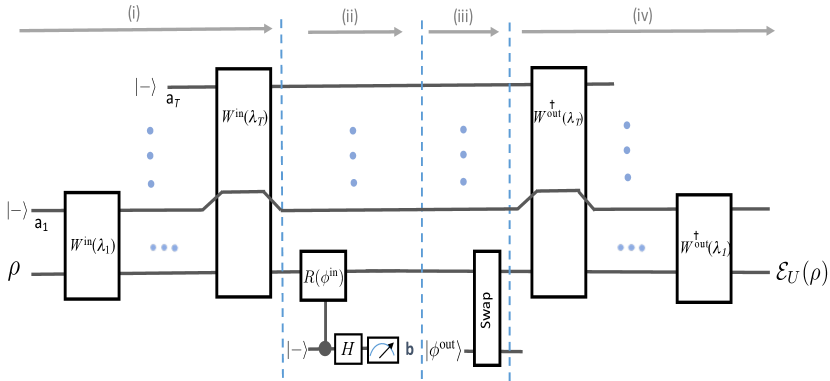
Figure 2: The generalized quantum circuit for emulating unitary $U$. .

Proof. We prove the theorem for the case of initial pure state $\rho=|\psi\rangle\langle\psi|$. The result for general mixed states follows from the joint concavity of Uhlmann fidelity.

Let $|\Theta(\boldsymbol{\lambda})\rangle$ be the joint state of the system and the ancillary qubits $a_{1}\cdots a_{T}$ at the end of step (i), for a particular choice of random parameters $\boldsymbol{\lambda}=(\lambda_{1},\cdots,\lambda_{T})$. This state is given by

$$|\Theta(\boldsymbol{\lambda})\rangle=\Big{[}W_{a_{T}}^{\text{in}}(\lambda_{T})\cdots W_{a_{1}}^{\text{in}}(\lambda_{1})\Big{]}|\psi\rangle\otimes|-\rangle^{\otimes T}\ .$$ (16)

Then, if we ignore the outcome of the measurement in step (ii), at the end of step (iii) the joint state of system and ancillary qubits $a_{1}\cdots a_{T}$, for this particular choice of random parameters $\boldsymbol{\lambda}$ is given by

$$|\phi^{\text{out}}\rangle\langle\phi^{\text{out}}|\otimes\textrm{Tr}_{S}(|\Theta(\boldsymbol{\lambda})\rangle\langle\Theta(\boldsymbol{\lambda})|)\ ,$$ (17)

where the partial trace is over the main system Hilbert space. Therefore, at the end of the algorithm the average joint state of the system and qubits $a_{1}\cdots a_{T}$ is given by

$$\sigma_{\text{fin}}=\sum_{\lambda_{1},\cdots,\lambda_{T}\in\Lambda}p(\lambda_{1})\cdots p(\lambda_{T})\ \left[{W_{a_{1}}^{\text{out}}}^{\dagger}(\lambda_{1})\cdots{W_{a_{T}}^{\text{out}}}^{\dagger}(\lambda_{T})\right]\Big{[}|\phi^{\text{out}}\rangle\langle\phi^{\text{out}}|\otimes\textrm{Tr}_{S}(|\Theta(\boldsymbol{\lambda})\rangle\langle\Theta(\boldsymbol{\lambda})|)\Big{]}\left[{W_{a_{T}}^{\text{out}}}(\lambda_{T})\cdots{W_{a_{1}}^{\text{out}}}(\lambda_{1})\right]\ ,$$ (18)

where we have averaged over iid random parameters $(\lambda_{1},\cdots,\lambda_{T})$, where each $\lambda_{i}\in\Lambda$ happens with probability $p(\lambda_{i})$.

Next, we look at $F_{\text{glob}}^{2}=\langle-|^{\otimes T}\langle\psi|U^{\dagger}\sigma_{\text{fin}}U|\psi\rangle|-\rangle^{\otimes T}$, that is the squared of the fidelity of the global output state $\sigma_{\text{fin}}$ with state $U|\psi\rangle|-\rangle^{\otimes T}$. Using Eq.(18) together with the facts that $U|\phi^{\text{in}}\rangle=|\phi^{\text{out}}\rangle$, and $(U\otimes I_{a})W^{\text{in}}_{a}(\lambda)(U^{\dagger}\otimes I_{a})=W^{\text{out}}_{a}(\lambda)\ ,$ and definition of $|\Theta(\boldsymbol{\lambda})\rangle$ in Eq.(16), we find that

$$F_{\text{glob}}^{2} =\sum_{\lambda_{1},\cdots,\lambda_{T}}\ p(\lambda_{1})\cdots p(\lambda_{T})\ \langle\Theta(\boldsymbol{\lambda})|\Big{[}|\phi^{\text{in}}\rangle\langle\phi^{\text{in}}|\otimes\textrm{Tr}_{S}(|\Theta(\boldsymbol{\lambda})\rangle\langle\Theta(\boldsymbol{\lambda})|)\Big{]}|\Theta(\boldsymbol{\lambda})\rangle\ .$$ (19)

Next, we note that

$$|\phi^{\text{in}}\rangle\langle\phi^{\text{in}}|\otimes\textrm{Tr}_{S}(|\Theta(\boldsymbol{\lambda})\rangle\langle\Theta(\boldsymbol{\lambda})|) =|\phi^{\text{in}}\rangle\langle\phi^{\text{in}}|\otimes\textrm{Tr}_{S}(P|\Theta(\boldsymbol{\lambda})\rangle\langle\Theta(\boldsymbol{\lambda})|P)+|\phi^{\text{in}}\rangle\langle\phi^{\text{in}}|\otimes\textrm{Tr}_{S}(P^{\perp}|\Theta(\boldsymbol{\lambda})\rangle\langle\Theta(\boldsymbol{\lambda})|P^{\perp})$$ (20a)

$$=\big{[}|\phi^{\text{in}}\rangle\langle\phi^{\text{in}}|\otimes I_{\textbf{a}}\big{]}|\Theta(\boldsymbol{\lambda})\rangle\langle\Theta(\boldsymbol{\lambda})|\big{[}|\phi^{\text{in}}\rangle\langle\phi^{\text{in}}|\otimes I_{\textbf{a}}\big{]}+|\phi^{\text{in}}\rangle\langle\phi^{\text{in}}|\otimes\textrm{Tr}_{S}(P^{\perp}|\Theta(\boldsymbol{\lambda})\rangle\langle\Theta(\boldsymbol{\lambda})|P^{\perp})\ ,$$ (20b)

where $P=|\phi^{\text{in}}\rangle\langle\phi^{\text{in}}|$, $P^{\perp}=I_{S}-P$, and $I_{S}$ and $I_{\textbf{a}}$ are, respectively, the identity operators on the system and the ancillary qubits $a_{1}\cdots a_{T}$. Using the fact that $\textrm{Tr}_{S}(P^{\perp}|\Theta(\boldsymbol{\lambda})\rangle\langle\Theta(\boldsymbol{\lambda})|P^{\perp})$ is a positive operator, we find

$$F_{\text{glob}}^{2} =\sum_{\lambda_{1},\cdots,\lambda_{T}}p(\lambda_{1})\cdots p(\lambda_{T})\ \langle\Theta(\boldsymbol{\lambda})|\Big{[}|\phi^{\text{in}}\rangle\langle\phi^{\text{in}}|\otimes\textrm{Tr}_{S}(|\Theta(\boldsymbol{\lambda})\rangle\langle\Theta(\boldsymbol{\lambda})|)\Big{]}|\Theta(\boldsymbol{\lambda})\rangle$$ (21a)

$$\geq\sum_{\lambda_{1},\cdots,\lambda_{T}}p(\lambda_{1})\cdots p(\lambda_{T})\ \langle\Theta(\boldsymbol{\lambda})|\big{[}|\phi^{\text{in}}\rangle\langle\phi^{\text{in}}|\otimes I_{\textbf{a}}\big{]}|\Theta(\boldsymbol{\lambda})\rangle\langle\Theta(\boldsymbol{\lambda})|\big{[}|\phi^{\text{in}}\rangle\langle\phi^{\text{in}}|\otimes I_{\textbf{a}}\big{]}|\Theta(\boldsymbol{\lambda})\rangle\$$ (21b)

$$=\sum_{\lambda_{1},\cdots,\lambda_{T}}p(\lambda_{1})\cdots p(\lambda_{T})\ \Big{(}\langle\Theta(\boldsymbol{\lambda})|\big{[}|\phi^{\text{in}}\rangle\langle\phi^{\text{in}}|\otimes I_{\textbf{a}}\big{]}|\Theta(\boldsymbol{\lambda})\rangle\Big{)}^{2}\ \ ,$$ (21c)

where $I_{\textbf{a}}$ is the identity operator on the qubits $a_{1}\cdots a_{T}$. Then, using the fact that for any distribution, the variance of a random variable is non-negative, we find that

$$F_{\text{glob}}^{2} \geq\sum_{\lambda_{1},\cdots,\lambda_{T}}p(\lambda_{1})\cdots p(\lambda_{T})\ \Big{(}\langle\Theta(\boldsymbol{\lambda})|\big{[}|\phi^{\text{in}}\rangle\langle\phi^{\text{in}}|\otimes I_{\textbf{a}}\big{]}|\Theta(\boldsymbol{\lambda})\rangle\Big{)}^{2}\$$ (22a)

$$\geq\Big{(}\sum_{\lambda_{1},\cdots,\lambda_{T}}p(\lambda_{1})\cdots p(\lambda_{T})\ \langle\Theta(\boldsymbol{\lambda})|\big{[}|\phi^{\text{in}}\rangle\langle\phi^{\text{in}}|\otimes I_{\textbf{a}}\big{]}|\Theta(\boldsymbol{\lambda})\rangle\Big{)}^{2}$$ (22b)

$$=\textrm{Tr}^{2}\left(|\phi^{\text{in}}\rangle\langle\phi^{\text{in}}|\sum_{\lambda_{1},\cdots,\lambda_{T}}p(\lambda_{1})\cdots p(\lambda_{T})\ \textrm{Tr}_{\textbf{a}}(|\Theta(\boldsymbol{\lambda})\rangle\langle\Theta(\boldsymbol{\lambda})|)\right)$$ (22c)

$$=p^{2}_{\text{erase}}(|\psi\rangle\langle\psi|)\ ,$$ (22d)

where $p_{\text{erase}}(|\psi\rangle\langle\psi|)$ is the probability that at the end of step (i) the reduced state of system is in state $|\phi^{\text{in}}\rangle$.

Finally, we note that the final state of system is obtained from state $\sigma_{\text{fin}}$, by tracing over the ancillary qubits, i.e. $\mathcal{E}_{U}(|\psi\rangle\langle\psi|)=\textrm{Tr}_{\text{\bf{a}}}(\sigma_{\text{glob}})$ . Then, using the monotonicity of Uhlmann fidelity under partial trace we find

$$\text{F}(\mathcal{E}_{U}(|\psi\rangle\langle\psi|),U|\psi\rangle\langle\psi|U^{\dagger})\geq F_{\text{glob}}\geq p_{\text{erase}}(|\psi\rangle\langle\psi|)\ .$$ (23)

Using the joint concavity of Uhlmann fidelity this proves the bound for arbitrary initial state $\rho$.

Next, using the definition $|\Theta(\boldsymbol{\lambda})\rangle=\Big{[}W_{a_{T}}^{\text{in}}(\lambda_{T})\cdots W_{a_{1}}^{\text{in}}(\lambda_{1})\Big{]}|\psi\rangle\otimes|-\rangle^{\otimes T}$, it can be easily shown that

$$\sum_{\lambda_{1},\cdots,\lambda_{T}}p(\lambda_{1})\cdots p(\lambda_{T})\textrm{Tr}_{\textbf{a}}(|\Theta(\boldsymbol{\lambda})\rangle\langle\Theta(\boldsymbol{\lambda})|)=\mathcal{W}^{T}(|\psi\rangle\langle\psi|),$$ (24a)

where

$$\mathcal{W}(\tau)=\sum_{\lambda\in\Lambda}p(\lambda)\ \textrm{Tr}_{a}\Big{(}W_{a}^{\text{in}}(\lambda)\Big{[}\tau\otimes|-\rangle\langle-|_{a}\Big{]}{W_{a}^{\text{in}}(\lambda)}^{\dagger}\Big{)}\ ,$$ (25)

and the partial trace is over qubit $a$. Therefore, we conclude that for any initial state $\rho$ it holds that $\text{F}(\mathcal{E}_{U}(\rho),U\rho U^{\dagger})\geq p_{\text{erase}}(\rho)=\langle\phi^{\text{in}}|\mathcal{W}^{T}(\rho)|\phi^{\text{in}}\rangle.$

In the above argument, we assumed we ignore the outcome of measurement in step (ii), which means that we do not care if the erasing has been successful or not. Now suppose we postselect to the cases where the erasing has been successful. In this case after the measurement the joint state of the system and ancillary qubits $a_{1}\cdots a_{T}$ is given by

$$\frac{1}{p_{\text{erase}}(|\psi\rangle\langle\psi|)}\times\sum_{\lambda_{1},\cdots,\lambda_{T}}p(\lambda_{1})\cdots p(\lambda_{T})\big{[}|\phi^{\text{in}}\rangle\langle\phi^{\text{in}}|\otimes I_{\textbf{a}}\big{]}|\Theta(\boldsymbol{\lambda})\rangle\langle\Theta(\boldsymbol{\lambda})|\big{[}|\phi^{\text{in}}\rangle\langle\phi^{\text{in}}|\otimes I_{\textbf{a}}\big{]},$$ (26)

where the factor $1/p_{\text{erase}}(|\psi\rangle\langle\psi|)$ is due to the postselection. Then, using an argument similar to the one we used before, we can show that the the squared of the fidelity of the final joint state of the system and qubits $a_{1}\cdots a_{T}$ at the end of the algorithm, with state $U|\psi\rangle\otimes|-\rangle^{\otimes T}$ is given by

$${F^{\text{post}}_{\text{glob}}}^{2} =\frac{1}{p_{\text{erase}}(|\psi\rangle\langle\psi|)}\times\sum_{\lambda_{1},\cdots,\lambda_{T}}p(\lambda_{1})\cdots p(\lambda_{T})\ \langle\Theta(\boldsymbol{\lambda})|\big{[}|\phi^{\text{in}}\rangle\langle\phi^{\text{in}}|\otimes I_{\textbf{a}}\big{]}|\Theta(\boldsymbol{\lambda})\rangle\langle\Theta(\boldsymbol{\lambda})|\big{[}|\phi^{\text{in}}\rangle\langle\phi^{\text{in}}|\otimes I_{\textbf{a}}\big{]}|\Theta(\boldsymbol{\lambda})\rangle\$$ (27a)

$$=\frac{1}{p_{\text{erase}}(|\psi\rangle\langle\psi|)}\times\sum_{\lambda_{1},\cdots,\lambda_{T}}p(\lambda_{1})\cdots p(\lambda_{T})\ \Big{(}\langle\Theta(\boldsymbol{\lambda})|\big{[}|\phi^{\text{in}}\rangle\langle\phi^{\text{in}}|\otimes I_{\textbf{a}}\big{]}|\Theta(\boldsymbol{\lambda})\rangle\Big{)}^{2}\ ,$$ (27b)

Then, using Eq.(22), we find

$${F^{\text{post}}_{\text{glob}}}^{2} \geq\frac{p^{2}_{\text{erase}}(|\psi\rangle\langle\psi|)}{p_{\text{erase}}(|\psi\rangle\langle\psi|)}=p_{\text{erase}}(|\psi\rangle\langle\psi|).$$ (28)

This means that if we postselect to the cases where erasing has been successful, then

$$F(U|\psi\rangle\langle\psi|U^{\dagger},\tilde{\rho}_{\text{post}})\geq F^{\text{post}}_{\text{glob}}\geq\sqrt{p_{\text{erase}}(|\psi\rangle\langle\psi|)}.$$ (29)

 

Appendix B Runtime and error analysis

In this section we first study the runtime and the error in the output of the algorithm, assuming we run the quantum circuit in Fig. 1 with ideal controlled-reflections $R_{a}(k)$. Then, we consider the runtime and error in the actual algorithm, where we use the given copies of sample states to simulate the controlled-reflections.

B.1 Algorithm with perfect controlled-reflections

Let $\mathcal{E}_{U}$ be the quantum channel that describes the overall effect of the circuit in Fig.(1) on the system, in the case where we ignore the outcome of measurement in step (ii), and where we use ideal controlled-reflections in the circuit. Let $\|\cdot\|_{1}$ be the $l_{1}$-norm, defined as the sum of the singular values of the operator. Then,

Theorem 2

Suppose in the quantum circuit presented in Fig.(1) we choose

$$T\geq\frac{d\times\log(8\epsilon^{-2}_{\text{id}}d)}{1-|\lambda_{\mathcal{D}}|}\ ,$$ (30)

where $\lambda_{\mathcal{D}}$ is the eigenvalue of channel $\mathcal{D}(\cdot)=K^{-1}\sum_{k=1}^{K}e^{i\pi|\phi_{k}^{\text{in}}\rangle\langle\phi_{k}^{\text{in}}|}(\cdot)e^{i\pi|\phi_{k}^{\text{in}}\rangle\langle\phi_{k}^{\text{in}}|}$ which has the second largest magnitude. Then, for any input $\rho$ whose support is restricted to the input subspace $\mathcal{H}_{\text{in}}$, the output of the circuit satisfies $\|U\rho U^{\dagger}-\mathcal{E}_{U}(\rho)\|_{1}\leq\epsilon_{\text{id}}$.

Proof. We start with Eq.(5) proven in Appendix A,

$$F(\mathcal{E}_{U}(\rho),U\rho U^{\dagger})\geq\langle\phi_{1}^{\text{in}}|\mathcal{W}^{T}(\rho)|\phi_{1}^{\text{in}}\rangle\ .$$ (31)

Let $P^{\perp}_{\text{in}}=\Pi_{\text{in}}-P=\Pi_{\text{in}}-|\phi^{\text{in}}_{1}\rangle\langle\phi_{1}^{\text{in}}|$ be the projector to the $(d-1)$-dimensional subspace of $\mathcal{H}_{\text{in}}$ orthogonal to $|\phi^{\text{in}}_{1}\rangle$, and $\mathcal{P}^{\perp}_{\text{in}}(\cdot)=P^{\perp}_{\text{in}}(\cdot)P^{\perp}_{\text{in}}$. Using the definition $\mathcal{W}(\sigma)=P\sigma P+\mathcal{D}(P^{\perp}\sigma P^{\perp})$, it can be easily seen that for any state $\sigma$ whose support is restricted to $\mathcal{H}_{\text{in}}$, it holds that

$$\mathcal{P}^{\perp}_{\text{in}}\circ\mathcal{W}(\sigma)=\mathcal{P}^{\perp}_{\text{in}}\circ\mathcal{W}\circ\mathcal{P}^{\perp}_{\text{in}}(\sigma)=\mathcal{P}^{\perp}_{\text{in}}\circ\mathcal{D}\circ\mathcal{P}^{\perp}_{\text{in}}(\sigma)\ .$$ (32)

Furthermore, using the fact that under channels $\mathcal{W}$ and $\mathcal{D}$ any state $\rho$ whose support is restricted to $\mathcal{H}_{\text{in}}$ is mapped to a state with support restricted to this subspace, we find that

$$\mathcal{P}^{\perp}_{\text{in}}\circ\mathcal{W}^{T}(\rho)=\left[\mathcal{P}^{\perp}_{\text{in}}\circ\mathcal{D}\circ\mathcal{P}^{\perp}_{\text{in}}\right]^{T}(\rho)\ .$$ (33)

This implies

$$F(\mathcal{E}_{U}(\rho),U\rho U^{\dagger}) \geq\langle\phi_{1}^{\text{in}}|\mathcal{W}^{T}(\rho)|\phi_{1}^{\text{in}}\rangle$$ (34)

$$=1-\textrm{Tr}\left(P^{\perp}\mathcal{W}^{T}(\rho)\right)$$ (35)

$$=1-\textrm{Tr}\left(P^{\perp}_{\text{in}}\mathcal{W}^{T}(\rho)\right)$$ (36)

$$=1-\textrm{Tr}\left(\mathcal{P}_{\text{in}}^{\perp}\circ\mathcal{W}^{T}(\rho)\right)$$ (37)

$$=1-\textrm{Tr}\left(\left[\mathcal{P}_{\text{in}}^{\perp}\circ\mathcal{D}\circ\mathcal{P}_{\text{in}}^{\perp}\right]^{T}(\rho)\right)\ ,$$ (38)

where to get the third line we have used the fact that the support of $\mathcal{W}^{T}(\rho)$ is contained in $\mathcal{H}_{\text{in}}$, and to get the last line we have used Eq.(32).

It turns out that quantum operations $\mathcal{D}$ and $\mathcal{P}_{\text{in}}^{\perp}\circ\mathcal{D}\circ\mathcal{P}_{\text{in}}^{\perp}$ have several nice properties which simplify the following analysis. In particular, they both have Hermitian matrix representations: Let $\{F_{\mu}:\mu=1\cdots d^{2}\}$ be an orthonormal basis for the operator space acting on $\mathcal{H}_{\text{in}}$, such that $\textrm{Tr}(F^{\dagger}_{\mu}F_{\nu})=\delta_{\mu,\nu}$. Consider the matrix representation of $\mathcal{D}$ and $\mathcal{P}_{\text{in}}^{\perp}\circ\mathcal{D}\circ\mathcal{P}_{\text{in}}^{\perp}$ on $\mathcal{H}_{\text{in}}$, i.e. the matrices $D_{\mu,\nu}=\textrm{Tr}(F^{\dagger}_{\mu}\mathcal{D}(F_{\nu}))$ and $D_{\mu,\nu}^{\perp}=\textrm{Tr}(F^{\dagger}_{\mu}\ \mathcal{P}_{\text{in}}^{\perp}\circ\mathcal{D}\circ\mathcal{P}_{\text{in}}^{\perp}(F_{\nu}))$, respectively. Then, the fact that any reflection $e^{i\pi|\phi\rangle\langle\phi|}$ is a Hermitian operator, implies that these matrices are both Hermitian (Note that the matrix representation of channel $\mathcal{W}$ is not Hermitian). Let $\lambda_{\perp}$ be the largest eigenvalue of $\mathcal{P}^{\perp}\circ\mathcal{D}\circ\mathcal{P}^{\perp}$. It follows that for any $T$, the map $\left[\mathcal{P}_{\text{in}}^{\perp}\circ\mathcal{D}\circ\mathcal{P}_{\text{in}}^{\perp}\right]^{T}$ has also a Hermitian matrix representation, and its largest eigenvalue is $\lambda^{T}_{\perp}$. This implies

$$\textrm{Tr}\left(\left[\mathcal{P}_{\text{in}}^{\perp}\circ\mathcal{D}\circ\mathcal{P}_{\text{in}}^{\perp}\right]^{T}(\rho)\right) =\textrm{Tr}\left(P^{\perp}_{\text{in}}\left[\mathcal{P}_{\text{in}}^{\perp}\circ\mathcal{D}\circ\mathcal{P}_{\text{in}}^{\perp}\right]^{T}(\rho)\right)$$ (39a)

$$\leq\textrm{Tr}\left(P^{\perp}_{\text{in}}\left[\mathcal{P}_{\text{in}}^{\perp}\circ\mathcal{D}\circ\mathcal{P}_{\text{in}}^{\perp}\right]^{T}(P^{\perp}_{\text{in}})\right)$$ (39b)

$$\leq|\lambda_{\perp}|^{T}\times\textrm{Tr}(P^{\perp}_{\text{in}})$$ (39c)

$$=|\lambda_{\perp}|^{T}\times(d-1)\ ,$$ (39d)

where to get the first line we use the fact that for any $X$, $P_{\text{in}}\mathcal{P}_{\text{in}}(X)=\mathcal{P}_{\text{in}}(X)$, and to get the third line we use the fact that $\lambda_{\perp}^{T}$ is the largest eigenvalue of $\mathcal{P}_{\text{in}}^{\perp}\circ\mathcal{D}\circ\mathcal{P}_{\text{in}}^{\perp}$, which implies for any $X$, $\textrm{Tr}\left(X^{\dagger}\left[\mathcal{P}_{\text{in}}^{\perp}\circ\mathcal{D}\circ\mathcal{P}_{\text{in}}^{\perp}\right]^{T}(X)\right)\leq\textrm{Tr}(X^{\dagger}X)|\lambda_{\perp}|^{T}$.

Putting this into Eq.(34) we find that

$$F(\mathcal{E}_{U}(\rho),U\rho U^{\dagger}) \geq 1-\textrm{Tr}\left(\left[\mathcal{P}^{\perp}\circ\mathcal{D}\circ\mathcal{P}^{\perp}\right]^{T}(\rho)\right)\geq 1-d\times|\lambda_{\perp}|^{T}\ .$$ (40)

Next, we use this bound together with the Fuchs-van de Graaf inequality, to bound the trace distance of $\mathcal{E}_{U}(\rho)$ and $U\rho U^{\dagger}$. We find

$$\big{\|}\mathcal{E}_{U}(\rho)-U\rho U^{\dagger}\big{\|}_{1} \leq 2\sqrt{1-F^{2}(\mathcal{E}_{U}(\rho),U\rho U^{\dagger})}\leq 2\sqrt{2}\sqrt{1-F(\mathcal{E}_{U}(\rho),U\rho U^{\dagger})}$$ (41)

$$\leq 2\sqrt{2d\times|\lambda_{\perp}|^{T}}\ .$$ (42)

This means that to achieve error $\epsilon_{\text{id}}$ in trace distance, it is sufficient to have

$$T\geq\frac{\log(8\epsilon^{-2}_{\text{id}}d)}{\log|\lambda|^{-1}_{\perp}}\ .$$ (43)

In the following we prove

$$|\lambda_{\perp}|\leq 1-\frac{1-|\lambda_{\mathcal{D}}|}{d}\ .$$ (44)

This together with the fact that $\log(1+x)\leq x$ for $x>-1$, implies

$$\frac{d}{1-|\lambda_{\mathcal{D}}|}\geq\frac{1}{\log|\lambda|^{-1}_{\perp}}\ .$$ (45)

Therefore, using Eq.(43), we conclude that if we choose $T$ such that

$$T\geq\frac{d\times\log(8\epsilon^{-2}_{\text{id}}d)}{1-|\lambda_{\mathcal{D}}|}\ ,$$ (46)

then $\big{\|}\mathcal{E}_{U}(\rho)-U\rho U^{\dagger}\big{\|}_{1}\leq\epsilon_{\text{id}}$.

Bound on the maximum eigenvalue of $\mathcal{P}_{\text{in}}^{\perp}\circ\mathcal{D}\circ\mathcal{P}_{\text{in}}^{\perp}$

To complete the proof, in the following we prove Eq.(44), which is a bound on $\lambda_{\perp}$, the largest eigenvalue of $\mathcal{P}_{\text{in}}^{\perp}\circ\mathcal{D}\circ\mathcal{P}_{\text{in}}^{\perp}$. Recall that $\mathcal{P}_{\text{in}}^{\perp}\circ\mathcal{D}\circ\mathcal{P}_{\text{in}}^{\perp}$ and $\mathcal{D}$ both have Hermitian matrix representations. This means that $\mathcal{D}$ has a spectral decomposition as $\mathcal{D}(X)=\sum_{\mu}\lambda_{\mu}M^{\dagger}_{\mu}\textrm{Tr}(M_{\mu}X)$, where each $\lambda_{\mu}$ and $M^{\dagger}_{\mu}$ are, respectively, the eigenvalue of $\mathcal{D}$ and its corresponding eigenvector, and $\textrm{Tr}(M^{\dagger}_{\mu}M_{\nu})=\delta_{\mu,\nu}$. Then, (the absolute value of) the maximum eigenvalue of $\mathcal{P}_{\text{in}}^{\perp}\circ\mathcal{D}\circ\mathcal{P}_{\text{in}}^{\perp}$ is given by

$$|\lambda_{\perp}|=\underset{X}{\textrm{max}}\frac{\left|\textrm{Tr}(X^{\dagger}\mathcal{P}_{\text{in}}^{\perp}\circ\mathcal{D}\circ\mathcal{P}_{\text{in}}^{\perp}(X)\right|}{\textrm{Tr}(X^{\dagger}X)}=\underset{X}{\textrm{max}}\left|\sum_{\mu}\lambda_{\mu}\frac{\left|\textrm{Tr}(M_{\mu}P_{\text{in}}^{\perp}XP_{\text{in}}^{\perp})\right|^{2}}{\textrm{Tr}(X^{\dagger}X)}\right|\ .$$ (47)

Note that the Hermiticity of $\mathcal{D}$ implies that its eigenvectors form an orthonormal basis, and so

$$\sum_{\mu}\left|\textrm{Tr}(M_{\mu}P_{\text{in}}^{\perp}XP_{\text{in}}^{\perp})\right|^{2}=\textrm{Tr}^{2}(P_{\text{in}}^{\perp}X^{\dagger}P_{\text{in}}^{\perp}XP_{\text{in}}^{\perp})\ .$$ (48)

Then, using the fact that the operator $\Pi_{\text{in}}/\sqrt{d}$ is the only (normalized) eigenvector of $\mathcal{D}$ with eigenvalue 1, we find

$$|\lambda_{\perp}|=\underset{X}{\textrm{max}}\left|\sum_{\mu}\lambda_{\mu}\frac{\left|\textrm{Tr}(M_{\mu}P_{\text{in}}^{\perp}XP_{\text{in}}^{\perp})\right|^{2}}{\textrm{Tr}(X^{\dagger}X)}\right|\leq\underset{X}{\textrm{max}}\left[\frac{|\textrm{Tr}(P_{\text{in}}^{\perp}XP_{\text{in}}^{\perp})|^{2}}{d\times\textrm{Tr}(X^{\dagger}X)}+|\lambda_{\mathcal{D}}|\frac{\textrm{Tr}(P_{\text{in}}^{\perp}X^{\dagger}P_{\text{in}}^{\perp}XP_{\text{in}}^{\perp})-|\textrm{Tr}(P_{\text{in}}^{\perp}XP_{\text{in}}^{\perp})|^{2}\times d^{-1}}{\textrm{Tr}(X^{\dagger}X)}\right]\ ,$$ (49)

where $\lambda_{\mathcal{D}}$ is the second largest eigenvalue of $\mathcal{D}$ (in magnitude). This implies

$$|\lambda_{\perp}|\leq\underset{X}{\textrm{max}}\left[\frac{|\textrm{Tr}(XP_{\text{in}}^{\perp})|^{2}}{d\times\textrm{Tr}(X^{\dagger}X)}\times(1-|\lambda_{\mathcal{D}}|)+|\lambda_{\mathcal{D}}|\right].$$ (50)

Then, using the Cauchy-Shwarz inequality we find

$$|\lambda_{\perp}|\leq\underset{X}{\textrm{max}}\left[\frac{\textrm{Tr}(XX^{\dagger})\textrm{Tr}(P_{\text{in}}^{\perp})}{d\times\textrm{Tr}(X^{\dagger}X)}\times(1-|\lambda_{\mathcal{D}}|)+|\lambda_{\mathcal{D}}|\right]=1-\frac{1-|\lambda_{\mathcal{D}}|}{d}\ ,$$ (51)

where we have used the fact that $\textrm{Tr}(P_{\text{in}}^{\perp})=d-1$ . This completes the proof of Eq.(44) and theorem 2.   

B.2 Total error in the actual algorithm with simulated controlled-reflections

As we showed in the previous section, in the idealized case where we are given perfect controlled-reflections by choosing

$$T\geq T(d,\epsilon_{\text{id}})\equiv\frac{d\log(8\epsilon^{-2}_{\text{id}}d)}{1-|\lambda_{\mathcal{D}}|}\ ,$$ (52)

we can implement the transformation $|\psi\rangle\rightarrow U|\psi\rangle$ on any initial state $|\psi\rangle\in\mathcal{H}_{\text{in}}$ with error less than or equal to $\epsilon_{\text{id}}$ in trace distance. But, in the main algorithm we need to simulate the controlled-reflections using the given copies of the sample states.

In the Appendix C we show that using $n$ copies of state $|\phi\rangle$ we can implement the unitary $e^{i\pi|\phi\rangle\langle\phi|}$, or its controlled version, $|0\rangle\langle 0|\otimes I+|1\rangle\langle 1|\otimes e^{i\pi|\phi\rangle\langle\phi|}$, with error $\mathcal{O}(1/n)$ in trace distance, and in time $\mathcal{O}(\log D\times n\log n)=\tilde{\mathcal{O}}(\log D\times n)$, where $\tilde{\mathcal{O}}$ suppresses more slowly-growing terms. In other words, to achieve the error of order $\epsilon_{\text{ref}}$ in simulating each controlled-reflection we need time of order $\tilde{\mathcal{O}}(\epsilon^{-1}_{\text{ref}}\times\log D)$, and $\tilde{\mathcal{O}}(\epsilon^{-1}_{\text{ref}})$ copies of the corresponding state.

Given that the circuit requires $4T+1$ controlled-reflection, it follows that we can implement the transformation $|\psi\rangle\rightarrow U|\psi\rangle$ , with the total error less than or equal to

$$\epsilon_{\text{tot}}=[4T(d,\epsilon_{\text{id}})+1]\times\epsilon_{\text{ref}}+\epsilon_{\text{id}}\ ,$$ (53)

in the total time

$$t_{\text{tot}}=[4T(d,\epsilon_{\text{id}})+1]\times\tilde{\mathcal{O}}(\epsilon^{-1}_{\text{ref}}\times\log D),$$ (54)

and using the total number of input-output sample pairs

$$N_{\text{tot}}=[4T(d,\epsilon_{\text{id}})+1]\times\epsilon^{-1}_{\text{ref}}\ .$$ (55)

Choosing $\epsilon_{\text{id}}$ and $\epsilon_{\text{ref}}$ such that $T(d,\epsilon_{\text{id}})\times\epsilon_{\text{ref}}=\epsilon_{\text{id}}=\epsilon$, we find that the transformation $|\psi\rangle\rightarrow U|\psi\rangle$ can be implemented with the total error less than or equal to $\epsilon$, in the total time

$$t_{\text{tot}}=\tilde{\mathcal{O}}\left(\frac{d^{2}\epsilon^{-1}\log D}{(1-|\lambda_{\mathcal{D}}|)^{2}}\right),$$ (56)

and using the total number of input-output sample pairs

$$N_{\text{tot}}=\tilde{\mathcal{O}}\left(\frac{d^{2}\epsilon^{-1}}{(1-|\lambda_{\mathcal{D}}|)^{2}}\right).$$ (57)

Appendix C An efficient quantum circuit for exponentiating a density operator

In this section, we introduce an explicit simple quantum circuit that uses multiple copies of state $\sigma$, to simulate the unitary $e^{-it\sigma}$, or its controlled version $|0\rangle\langle 0|\otimes I+|1\rangle\langle 1|\otimes e^{-it\sigma}$, for any real $t$. The circuit works based on the density matrix exponentiation technique of Lloyd et al. (2014).

Let $S$ be the SWAP operator acting on the system and an ancillary system with equal Hilbert space dimensions, such that $S|\mu\rangle|\nu\rangle=|\nu\rangle|\mu\rangle$, for any pair of states $|\mu\rangle$, and $|\nu\rangle$. Note that $S$ is a Hermitian unitary operator. Then, as it is observed in Ref.(Lloyd et al. (2014)),

$$\textrm{Tr}_{\text{RF}}\left(e^{-i\Delta tS}[\rho\otimes\sigma]e^{i\Delta tS}\right)=\rho+i\Delta t[\rho,\sigma]+\mathcal{O}(\Delta t^{2})=e^{-i\sigma\Delta t}\rho e^{i\sigma\Delta t}+\mathcal{O}(\Delta t^{2})\ ,$$ (58)

where the partial trace is over the system with state $\sigma$ (which can be interpreted as a quantum reference frame Marvian and Mann (2008); Bartlett et al. (2007)). Then, choosing sufficiently small $\Delta t$, and repeating the above procedure for $t/\Delta t$ times with $t/\Delta t$ copies of state $\sigma$, we can simulate the unitary $e^{-i\sigma t}$ with arbitrary accuracy.

In the following section we present a new simple and efficient algorithm for simulating the unitary $e^{-i\theta S}$ for arbitrary $\theta$, with error $\epsilon$ and in time $\mathcal{O}(\log{(D)\times\log(1/\epsilon)})$. Therefore, if we use this algorithm together with the above method, using one copy of state $\sigma$ we can simulate the unitary $e^{-i\sigma\Delta t}$ with the total error of order $\Delta t^{2}+\epsilon$, and in time $\mathcal{O}(\log{(D)\times\log(1/\epsilon)})$. Then, having $n$ copies of state $\sigma$, to simulate the unitary $e^{-i\sigma t}$ we can choose $\Delta t=t/n$ and use each copy to simulate $e^{-i\sigma\Delta t}$. In this case the total error is

$$\epsilon_{\text{tot}}=\mathcal{O}\big{(}n\times(\epsilon+\Delta t^{2})\big{)}=\mathcal{O}\big{(}n\epsilon+\frac{t^{2}}{n}\big{)}\ ,$$ (59)

and the total runtime is

$$t_{\text{tot}}=\mathcal{O}(\log(D)\times\log(1/\epsilon)\times n)\ ,$$ (60)

where $\epsilon$ is the error in implementing the unitary $e^{-i\Delta tS}$. Choosing $\epsilon=\frac{1}{n^{2}}$, we find that using $n$ copies of state $\sigma$ we can simulate unitary $e^{-i\sigma t}$, with the total error of order $\epsilon_{\text{tot}}=\mathcal{O}(\frac{t^{2}+1}{n})$ in trace distance, and in time of order $\mathcal{O}\big{(}\log(D)\times n\log(n)\big{)}$ .

Furthermore, using Eq.(58), it can be easily shown that if instead of the unitary $e^{-i\Delta tS}$ we implement its controlled version, i.e. the unitary $|0\rangle\langle 0|\otimes I+|1\rangle\langle 1|\otimes e^{-iS\Delta t}$, then we can simulate the controlled version of $e^{-i\sigma\Delta t}$, i.e. the unitary $|0\rangle\langle 0|\otimes I+|1\rangle\langle 1|\otimes e^{-i\sigma\Delta t}$. To implement the unitary $|0\rangle\langle 0|\otimes I+|1\rangle\langle 1|\otimes e^{-iS\Delta t}$, we note that

$$e^{-iS_{c}\Delta t}=|0\rangle\langle 0|\otimes e^{-i\Delta t}I+|1\rangle\langle 1|\otimes e^{-iS\Delta t},$$ (61)

where $S_{c}=|0\rangle\langle 0|\otimes I+|1\rangle\langle 1|\otimes S\ ,$ is the controlled-SWAP unitary. Using the algorithm presented in the next section, we can efficiently simulate this unitary with error $\epsilon$ in time $\mathcal{O}(\log{(D)\times\log(1/\epsilon)})$. Then, if after applying $e^{-iS_{c}\Delta t}$ we apply $e^{i\sigma_{z}\Delta t/2}$ on the control qubit, we implement the desired unitary $|0\rangle\langle 0|\otimes I+|1\rangle\langle 1|\otimes e^{-iS\Delta t}$, up to a global phase.

Therefore, having $n$ copies of state $\sigma$ to simulate the unitary $|0\rangle\langle 0|\otimes I+|1\rangle\langle 1|\otimes e^{-i\sigma t}$, we first apply the unitary $e^{-iS_{c}t/n}$ to the system, the control qubit and each one of these $n$ copies, and then apply the the unitary $e^{i\sigma_{z}t/2}$ on the control qubit. It follows that we can implement the unitary $|0\rangle\langle 0|\otimes I+|1\rangle\langle 1|\otimes e^{-i\sigma t}$,with the total error less than or equal to $\mathcal{O}(\frac{t^{2}+1}{n})$ in time $\mathcal{O}\big{(}\log(D)\times n\log(n)\big{)}$ .

We conclude that

Theorem 3

Using $n$ copies of an unknown state $\sigma$ we can simulate the unitary $e^{-i\sigma t}$, or its controlled version $|0\rangle\langle 0|\otimes I+|1\rangle\langle 1|\otimes e^{-i\sigma\Delta t}$ in time $\mathcal{O}\big{(}\log(D)\times n\log(n)\big{)}$, with error $\mathcal{O}(\frac{t^{2}+1}{n})$ in trace distance.

C.1 An efficient quantum circuit for simulating the time evolution generated by the (controlled-)SWAP Hamiltonian

In this section we present a simple quantum circuit to simulate the time evolution generated by the SWAP Hamiltonian on a pair of systems whose Hilbert spaces have equal dimension. This algorithm simulates any such unitary with error less than or equal to $\epsilon$ (in trace distance) in time $\mathcal{O}(\log(D)\times\log(1/\epsilon))$, where $D$ is the dimension of the Hilbert space of each system. We also explain how the same idea can be used to simulate the controlled-SWAP Hamiltonian as well.

Let $S$ be the SWAP operator acting on a pair of systems $A$ and $B$. The fact that $S^{2}$ is the identity operator implies that any unitary generated by $S$ has the following form

$$e^{iS\theta}=\cos\theta\ I+i\sin\theta\ S\ ,$$ (62)

where $I$ is the identity operator on the joint system. To simulate a general unitary in this form we first implement $S_{c}$, the controlled-SWAP unitary defined by

$$S_{c}=|0\rangle\langle 0|_{c}\otimes I+|1\rangle\langle 1|_{c}\otimes S\ ,$$ (63)

where $c$ is the label for an ancillary qubit. This unitary can be efficiently implemented, using controlled-SWAP gates for qubits, also known as Fredkin gate Nielsen and Chuang (2000). To implement $S_{c}$ in this way, we need to apply $\mathcal{O}(\log(D))$ Fredkin gates, where each Fredkin gate is controlled by the ancillary qubit $c$, and is acting on a qubit in systems $A$, and its corresponding qubit in system $B$.

Then, using the controlled-SWAP operator $S_{c}$, we can easily implement the unitary $e^{iS\theta}$, for any $\theta$: First, we prepare the ancillary qubit in state $\cos\theta|0\rangle+i\sin\theta|1\rangle$ and apply the controlled-SWAP $S_{c}$ to the ancillary qubit and the systems $A$ and $B$ in an arbitrary initial state $|\gamma\rangle$. This yields

$$S_{c}(\cos\theta|0\rangle+i\sin\theta|1\rangle)\otimes|\gamma\rangle=\cos\theta\ |0\rangle|\gamma\rangle+i\sin\theta\ |1\rangle S|\gamma\rangle\ .$$ (64)

Next, we measure the ancillary qubit in $\{(|0\rangle\pm|1\rangle)/\sqrt{2}\}$ basis. Then, with probability 1/2 we project this qubit to state $(|0\rangle+|1\rangle)/\sqrt{2}$. In this case we have implemented the desired transformation on the systems, i.e. we get state

$$\frac{|0\rangle+|1\rangle}{\sqrt{2}}(\cos\theta|\gamma\rangle+i\sin\theta S|\gamma\rangle)=\frac{|0\rangle+|1\rangle}{\sqrt{2}}e^{i\theta S}|\gamma\rangle.$$ (65)

On the other hand, with probability $1/2$ the state of conrtol qubit is projected to $(|0\rangle-|1\rangle)/\sqrt{2}$, in which case we get state

$$\frac{|0\rangle-|1\rangle}{\sqrt{2}}(\cos\theta\ |\gamma\rangle-i\sin\theta\ S|\gamma\rangle)=\frac{|0\rangle-|1\rangle}{\sqrt{2}}\otimes e^{-i\theta S}|\gamma\rangle.$$ (66)

Therefore, in the latter case instead of the desired unitary $e^{i\theta S}$ we have implemented the unitary $e^{-i\theta S}$. But because these unitaries all commute with each other, we can correct this error: we repeat the above process and this time we try to implement the unitary $e^{i2\theta S}$, by preparing the ancilla in state $\cos 2\theta\ |0\rangle+i\sin 2\theta\ |1\rangle$, instead of $\cos\theta\ |0\rangle+i\sin\theta\ |1\rangle$. Then, again with probability 1/2 we will be successful and implement the overall unitary $e^{i2\theta S}e^{-i\theta S}=e^{i\theta S}$, as we desired. On the other hand, with probability 1/2 we are unsuccessful in which case we have implemented the overall unitary $e^{-iS\theta}e^{-iS2\theta}=e^{-iS3\theta}$ . In this case we repeat the above process and try to implement the unitary $e^{iS4\theta}$, by preparing the ancillary qubit in state $\cos 4\theta\ |0\rangle+i\sin 4\theta\ |1\rangle$.

Repeating this process for $r$ times we achieve the desired unitary with probability $1-1/2^{r}$. Since each time we need to apply $S_{c}$, which takes time of order $\log D$, we find that the total time it takes to implement $e^{iS\theta}$ with error $\epsilon$ is $\mathcal{O}(\log{(D)\times\log(1/\epsilon)})$.

Finally, note that we can use a similar method to implement the unitary

$$e^{i\theta S_{c}}=|0\rangle\langle 0|\otimes e^{i\theta}I+|1\rangle\langle 1|\otimes e^{iS\theta}=\cos\theta I+i\sin\theta S_{c}.$$ (67)

To implement this unitary, it suffices to replace the Fredkin gates in the above algorithm, with controlled-Fredkin gates, i.e. controlled-controlled-SWAP gates each of which acts on the a pair of qubits in systems $A$ and $B$, and is controlled by the original control qubit and the anicallry qubit that we need to implement the above procedure.

Appendix D Generalizations

In this section we discuss several generalizations of the results presented in the paper. These generalizations are summarized in Sec.(IV) of the paper.

D.1 Input-output pairs of mixed states

The algorithm presented in the paper assumes the given samples of the input-output pairs are all pure states. However, as we explained at the end of Sec.(III.1) this algorithm can be generalized to the case where the sample states contain mixed states. It can be easily shown that, as long as the sample input states $S_{\text{in}}=\{\rho^{\text{in}}_{k},k=1,\cdots K\}$ contain (at least) one state close to a pure state, we can still coherently erase the sate of system and push it into this pure state. Then, we can emulate the action of the unknown unitary $U$, using the same approach we used in the original algorithm.

Let $\mathcal{H}_{\text{in}}$ be the subspace spanned by the union of the support of density operators in $S_{\text{in}}=\{\rho^{\text{in}}_{k},k=1,\cdots K\}$. Then, having copies of sample input-output states in $S_{\text{in}}$ and $S_{\text{out}}$, we can determine the action of $U$ on any state in $\mathcal{H}_{\text{in}}$, if and only if the set $S_{\text{in}}$ generates the full matrix algebra on $\mathcal{H}_{\text{in}}$. Therefore, in the following we naturally assume this condition is satisfied.

To erase the state of system coherently we use controlled-translations with respect to the given sample states, i.e. the unitaries

$$T_{a}(k,t)=|0\rangle\langle 0|_{a}\otimes I+|1\rangle\langle 1|_{a}\otimes e^{-i\rho_{k}t}\ ,$$ (68)

where we have suppressed in and out superscript in both sides. As we discussed in Appendix C, using the given copies of sample states we can efficiently simulate these unitaries. Recall that the input set $S_{\text{in}}$ (and hence $S_{\text{out}}$) contains at least one pure state. Without loss of generality, let $\rho_{1}^{\text{in}}$ and $\rho_{1}^{\text{out}}=U\rho_{1}^{\text{in}}U^{\dagger}$ be the pure state in the sample set $S_{\text{in}}$ and its corresponding output state in the set $S_{\text{out}}$, respectively. Then instead of unitaries $W_{a}(k)=R_{a}(k)H_{a}R_{a}(1)$ used in the original algorithm, we use unitaries $W_{a}(k,t)=T_{a}(k,t)H_{a}T_{a}(1,\pi)$, where we have suppressed in and out superscripts, and choose $k$ and $t$ uniformly at random from the sets $1,\cdots,K$ and $[0,1]$, respectively. Then, it can be easily shown that state $\rho_{\text{in}}^{1}=|\phi^{\text{in}}_{1}\rangle\langle\phi^{\text{in}}_{1}|$ is the unique fixed point state of channel $\mathcal{W}=1/K\sum_{k=1}^{K}\int_{0}^{1}dt\textrm{Tr}_{a}\big{(}W_{a}^{\text{in}}(k,t)[\tau\otimes|-\rangle\langle-|_{a}]{W_{a}^{\text{in}}}^{\dagger}(k,t)\big{)}$ inside $\mathcal{H}_{\text{in}}$. It follows that we can coherently erase the state of system, and therefore, using the same technique we used in the main algorithm, we can emulate the action of unitary $U$.

D.2 Emulating controlled unitaries

In many quantum algorithms, such as quantum phase estimation, one needs to implement the controlled version of a unitary $U$, i.e. the unitary $U^{c}\equiv|0\rangle\langle 0|\otimes I+|1\rangle\langle 1|\otimes U$. Can we modify the proposed algorithm to implement the controlled version of $U$ as well?

To answer this question, first note that if the only given resources are multiple copies of states in $S_{\text{in}}$ and $S_{\text{out}}$, it is impossible to distinguish between unitaries $U$ and $e^{i\theta}U$, for any phase $e^{i\theta}$. On the other hand, in general the controlled version of $U$ and $e^{i\theta}U$ are distinct unitaries, which are not equivalent up to a global phase. This means that even to specify what is the controlled version of $U$ we need extra resources that define and fix this global phase. For instance, we can use multiple copies of the input state $|\Phi^{\text{in}}\rangle=(\alpha|0\rangle+\beta|1\rangle)\otimes|\phi^{\text{in}}\rangle\ ,$ with $\alpha\neq 0$ and $\beta\neq 0$ and $|\phi^{\text{in}}\rangle\in\mathcal{H}_{\text{in}}$, together with copies of its corresponding output $|\Phi^{\text{out}}\rangle=U^{c}|\Phi^{\text{in}}\rangle$.

Therefore, in the following we assume in addition to the multiple copies of states in $S_{\text{in}}$ and $S_{\text{out}}$, we are also given multiple copies of states $|\Phi^{\text{in}}\rangle$ and $|\Phi^{\text{out}}\rangle$. Again, we naturally assume the set $S_{\text{in}}$ generates the full matrix algebra on $\mathcal{H}_{\text{in}}$. This together with the fact that $|\phi^{\text{in}}\rangle\in\mathcal{H}_{\text{in}}$ implies the set

$$\big{(}\ \{|0\rangle\langle 0|,|1\rangle\langle 1\}\otimes S_{\text{in}}\ \big{)}\cup\{|\Phi^{\text{in}}\rangle\langle\Phi^{\text{in}}|\}$$ (69)

generates the full matrix algebra on $\mathbb{C}^{2}\otimes\mathcal{H}_{\text{in}}$, where $\mathbb{C}^{2}$ denotes the Hilbert space of the controlled qubit. It follows that, given these resources we can now implement the algorithm proposed in the paper to emulate the controlled-unitary $U^{c}$ on $\mathbb{C}^{2}\otimes\mathcal{H}_{\text{in}}$. In other words, if instead of states in the sets $S_{\text{in}}$ and $S_{\text{out}}$ we choose states from the sets $\big{(}\{|0\rangle\langle 0|,|1\rangle\langle 1\}\otimes S_{\text{in}}\big{)}\cup\{|\Phi^{\text{in}}\rangle\langle\Phi^{\text{in}}|\}$ and $\big{(}\{|0\rangle\langle 0|,|1\rangle\langle 1\}\otimes S_{\text{out}}\big{)}\cup\{|\Phi^{\text{out}}\rangle\langle\Phi^{\text{out}}|\}$ respectively, we implement unitary $U^{c}$.

D.3 More efficient algorithm with prior information about samples

The algorithm presented in the paper does not assume any prior information about the sample input states, or the relation between them. On the other hand, as we show in the following, making some assumptions about the sample input states, we can emulate the unknown unitary more efficiently. Note that we do not assume any prior information about any single sample states; the assumption is only about the relation between them. More precisely, the assumption is about the pairwise inner product between the states in the input set.

The main idea behind this version of algorithm is again emulating via coherent erasing. We use the fact that by measuring the system in two conjugate bases, we can completely erase the state of system. Therefore, we assume we are given multiple copies of states in an orthonormal basis for the input subspace, and their corresponding output states. We also assume we are given multiple copies of one (or more) state in the conjugate basis, and their corresponding outputs. Then using these sample states we can simulate coherent measurements in both basis, and coherently erase the state of system.

Let $\{|\theta^{\text{in}}_{k}\rangle:k=0\cdots d-1\}$ be $d$ unknown orthonormal states in the $d$-dimensional input subspace $\mathcal{H}_{\text{in}}$, and

$$|\alpha^{\text{in}}_{j}\rangle=\frac{1}{\sqrt{d}}\sum^{d-1}_{k=0}e^{i2\pi kj/d}\ |\theta^{\text{in}}_{k}\rangle\ \ \ \ \ :\ j=0\cdots d-1\ ,$$ (70)

be the orthonormal basis for $\mathcal{H}_{\text{in}}$, which is conjugate to $\{|\theta^{\text{in}}_{k}\rangle:k=0\cdots d-1\}$. We assume we are given multiple copies of the input states $\{|\theta^{\text{in}}_{k}\rangle:k=0\cdots d-1\}$ and $\{|\alpha^{\text{in}}_{j}\rangle:j=0\cdots d-1\}$, and their corresponding output states $\{|\theta^{\text{out}}_{k}\rangle=U|\theta^{\text{in}}_{k}\rangle:k=0\cdots d-1\}$ and $\{|\alpha^{\text{out}}_{j}\rangle=U|\alpha^{\text{in}}_{j}\rangle:j=0\cdots d-1\}$. Note that, even if we are only given multiple copies of states $\{|\theta^{\text{in}}_{k}\rangle:\ k=0\cdots d-1\}$ and multiple copies of one of the states in $\{|\alpha^{\text{in}}_{k}\rangle:k=0\cdots d-1\}$, we can efficiently generate all states in this set (and similarly, for the set $\{|\alpha^{\text{out}}_{k}\rangle:k=0\cdots d-1\}$).

In the first step of this algorithm we perform a coherent measurement in $\{|\theta^{\text{in}}_{k}\rangle:k=0\cdots d-1\}$ basis. To do this we couple the system to an ancillary system with a $d-$dimensional Hilbert space. The ancillary system is initially prepared in the state $|\Gamma\rangle=\sqrt{d^{-1}}\sum_{t=0}^{d-1}|t\rangle$, where $\{|t\rangle:t=0\cdots d-1\}$ is a standard orthonormal basis. Then, we use the given copies of sample states $\{|\theta^{\text{in}}_{k}\rangle:k=0\cdots d-1\}$ to simulate the unitary

$$V^{\text{in}}_{P}=\sum_{k,t=0}^{d-1}e^{itk2\pi/d}|\theta^{\text{in}}_{k}\rangle\langle\theta^{\text{in}}_{k}|\otimes|t\rangle\langle t|=\sum_{t=0}^{d-1}e^{itP^{\text{in}}2\pi/d}\otimes|t\rangle\langle t|\ ,$$ (71)

where $P^{\text{in}}=\sum_{k=0}^{d-1}k|\theta^{\text{in}}_{k}\rangle\langle\theta^{\text{in}}_{k}|$. To efficiently simulate this unitary we first note that it has a decomposition as

$$V^{\text{in}}_{P}=\prod_{k=0}^{d-1}\sum_{t=0}^{d-1}e^{it|\theta^{\text{in}}_{k}\rangle\langle\theta^{\text{in}}_{k}|2\pi k/d}\otimes|t\rangle\langle t|\ .$$ (72)

Therefore, to simulate $V^{\text{in}}_{P}$ we can simulate the (commuting) unitaries $\sum_{t=0}^{d-1}e^{it|\theta^{\text{in}}_{k}\rangle\langle\theta^{\text{in}}_{k}|2\pi k/d}\otimes|t\rangle\langle t|$, for $k=0,\cdots,d-1$. Each unitary $\sum_{t=0}^{d-1}e^{it|\theta^{\text{in}}_{k}\rangle\langle\theta^{\text{in}}_{k}|2\pi k/d}\otimes|t\rangle\langle t|$ can be efficiently simulated using the given copies of state $|\theta^{\text{in}}_{k}\rangle$. Using the results presented in Appendix C, this simulation can be done in time $\mathcal{O}(\log D)$, where $D$ is the dimension of the Hilbert space. Then, it follows from the decomposition of $V^{\text{in}}_{P}$ given by Eq.(72) that we can simulate $V^{\text{in}}_{P}$ in time $\mathcal{O}(d\log D)$, using the given copies of sample states $\{|\theta^{\text{in}}_{k}\rangle,\ k=0\cdots d-1\}$.

Applying the unitary $V^{\text{in}}_{P}$ to the system in state $|\psi\rangle\in\mathcal{H}_{\text{in}}$ and the ancillary system prepared in state $|\Gamma\rangle$, we get state

$$|\psi\rangle\otimes|\Gamma\rangle=\sum_{k=0}^{d-1}\psi_{k}|\theta^{\text{in}}_{k}\rangle\otimes|\Gamma\rangle\longrightarrow V^{\text{in}}_{P}|\psi\rangle\otimes|\Gamma\rangle=\sum_{k=0}^{d-1}\psi_{k}\ |\theta^{\text{in}}_{k}\rangle\otimes\frac{1}{\sqrt{d}}\sum_{t=0}^{d-1}e^{itk2\pi/d}|t\rangle\ ,$$ (73)

where we have used the decomposition $|\psi\rangle=\sum_{k=0}^{d-1}\psi_{k}|\theta^{\text{in}}_{k}\rangle$.

Then, performing quantum Fourier transform on the ancillary system we transform the joint state to

$$V^{\text{in}}_{P}|\psi\rangle\otimes|\Gamma\rangle=\sum_{k=0}^{d-1}\psi_{k}\ |\theta^{\text{in}}_{k}\rangle\otimes\sum_{t=0}^{d-1}e^{itk2\pi/d}|k\rangle\xrightarrow{\text{QFT}}\sum_{k=0}^{d-1}\psi_{k}\ |\theta^{\text{in}}_{k}\rangle\otimes|k\rangle\ .$$ (74)

Then, to erase the information in the system we implement the unitary

$$V^{\text{in}}_{Q}=\sum_{k,t=0}^{d-1}e^{itk2\pi/d}|\alpha^{\text{in}}_{k}\rangle\langle\alpha^{\text{in}}_{k}|\otimes|t\rangle\langle t|=\sum_{t=0}^{d-1}e^{itQ^{\text{in}}2\pi/d}\otimes|t\rangle\langle t|\ ,$$ (75)

where $Q^{\text{in}}=\sum_{l=0}^{d-1}l|\alpha^{\text{in}}_{l}\rangle\langle\alpha^{\text{in}}_{l}|$. Note that we can efficiently simulate $V^{\text{in}}_{Q}$, using a similar approach we used to simulate $V^{\text{in}}_{P}$.

Applying $V^{\text{in}}_{Q}$ to state in Eq.(74) we find

$$\sum_{k=0}^{d-1}\psi_{k}\ |\theta^{\text{in}}_{k}\rangle\otimes|k\rangle\longrightarrow V^{\text{in}}_{Q}\sum_{k=0}^{d-1}\psi_{k}\ |\theta^{\text{in}}_{k}\rangle\otimes|k\rangle=\sum_{k=0}^{d-1}\psi_{k}\ e^{ikQ^{\text{in}}2\pi/d}|\theta^{\text{in}}_{k}\rangle\otimes|k\rangle=|\theta^{\text{in}}_{0}\rangle\otimes\sum_{k=0}^{d-1}\psi_{k}\ |k\rangle\ ,$$ (76)

where we have used the fact that

$$e^{ikQ^{\text{in}}2\pi/d}|\theta^{\text{in}}_{k}\rangle=\sum_{l=0}^{d-1}e^{i2\pi lk/d}|\alpha^{\text{in}}_{l}\rangle\langle\alpha^{\text{in}}_{l}|\theta^{\text{in}}_{k}\rangle=\frac{1}{\sqrt{d}}\sum_{l=0}^{d-1}e^{i2\pi lk/d}e^{-i2\pi kl/d}|\alpha^{\text{in}}_{l}\rangle=|\theta^{\text{in}}_{0}\rangle.$$ (77)

Therefore, after these three steps for any input state $|\psi\rangle\in\mathcal{H}_{\text{in}}$ we have

$$\left[V^{\text{in}}_{Q}(I\otimes F_{\text{a}})V^{\text{in}}_{P}\right]|\psi\rangle|\Gamma\rangle=|\theta^{\text{in}}_{0}\rangle\otimes\sum_{k=0}^{d-1}\psi_{k}\ |k\rangle\ ,$$ (78)

where $F_{\text{a}}$ denotes the quantum Fourier transform on the ancillary system.

At this point we have completely erased the state of system and transferred all its information to the ancillary system. Now using a method similar to the one used in the main algorithm, we can transform this state to state $U|\psi\rangle|\Gamma\rangle$: We replace $|\theta^{\text{in}}_{0}\rangle$ with $|\theta^{\text{out}}_{0}\rangle$ and apply ${V^{\text{out}}_{P}}^{\dagger}(I\otimes F^{\dagger}_{\text{a}}){V^{\text{out}}_{Q}}^{\dagger}$ to state $|\theta^{\text{out}}_{0}\rangle\otimes\sum_{k=0}^{d-1}\psi_{k}\ |k\rangle$, where

$$V^{\text{out}}_{Q} =\sum_{k,t=0}^{d-1}e^{itk2\pi/d}|\alpha^{\text{out}}_{k}\rangle\langle\alpha^{\text{out}}_{k}|\otimes|t\rangle\langle t|=\sum_{t=0}^{d-1}e^{itQ^{\text{out}}2\pi/d}\otimes|t\rangle\langle t|\ ,$$ (79)

$$V^{\text{out}}_{P} =\sum_{k,t=0}^{d-1}e^{itk2\pi/d}|\theta^{\text{out}}_{k}\rangle\langle\theta^{\text{out}}_{k}|\otimes|t\rangle\langle t|=\sum_{t=0}^{d-1}e^{itP^{\text{out}}2\pi/d}\otimes|t\rangle\langle t|\ .$$ (80)

Note that these unitaries can be efficiently simulated using the same method we used to simulate the unitary $V_{P}^{\text{in}}$.

It follows that we can emulate the action of unitary $U$ on the input subspace in time $\mathcal{O}(d\log(D))$.

D.4 Approximate transformations

In the above discussions we always assumed there exists a unitary $U$ for which $U|\phi_{k}^{\text{in}}\rangle=|\phi_{k}^{\text{out}}\rangle$, for all $k=1,\cdots K$. Now suppose we only know that these transformations are possible approximately. I.e. there exists a constant $\delta>0$ and a unitary $U$ such that $\|U|\phi_{k}^{\text{in}}\rangle-|\phi_{k}^{\text{out}}\rangle\|\leq\delta$, for $k=1,\cdots,K$. Then, it can be easily shown that if we run the proposed algorithm on an input state $|\psi\rangle\in\mathcal{H}_{\text{in}}$, with the given sample input-output pairs, in the output we generate a quantum state whose trace distance from state $U|\psi\rangle$ is bounded by $\mathcal{O}(T\times\delta)=\delta\times\text{poly}(d)$. This follows form the fact that, under the above assumption, we can repeat the argument that is used to derive Eq.(4) from Eq.(3), and use $\|U|\phi_{1}^{\text{in}}\rangle-|\phi_{1}^{\text{out}}\rangle\|\leq\delta$ and $\|(U\otimes I_{a})W^{\text{in}}_{a}(k)(U^{\dagger}\otimes I_{a})-W^{\text{out}}_{a}(k)\|\leq 4\delta$, which follows from $\|U|\phi_{k}^{\text{in}}\rangle-|\phi_{k}^{\text{out}}\rangle\|\leq\delta$, for $k=1,\cdots,K$. This implies Eq.(4) is satisfied with an additional error of order $\mathcal{O}(T\delta)$, which proves the claim. Note that, for a general input-output sets $S_{\text{in}}$ and $S_{\text{out}}$ and a general input state $|\psi\rangle\in\mathcal{H}_{\text{in}}$, the lowest achievable error in this transformation is $\mathcal{O}(d\times\delta)$.

Appendix E Emulating projective measurements

In this section we consider the problem of emulating projective measurements. We assume we are given multiple copies of states that belong to different subspaces of the Hilbert space, with the labels which specify these subspaces. Then, we are interested to simulate the projective measurement that projects any given input state to one of these subspaces. Note that any projective measurement can be realized as a sequence of two-outcome measurements. Therefore, in the following we focus on implementing two-outcome measurements.

Consider the set of sample states $\{|\phi_{k}\rangle:1,\cdots,K\}$. We do not make any assumption about the sample states, or the relation between them. Let $\mathcal{H}_{\Pi}$ be the subspace spanned by these states, and $\Pi$ be the projector to this subspace. Assuming we are given multiple copies of each state in this set we are interested to implement the projective measurement described by the projectors $\{\Pi,I-\Pi\}$.

In the algorithm we use the controlled-reflections

$$R_{a}(k)=|0\rangle\langle 0|_{a}\otimes I+|1\rangle\langle 1|_{a}\otimes e^{i\pi|\phi_{k}\rangle\langle\phi_{k}|}\ .$$ (81)

As we explained in Appendix C, using $n$ copies of state $|\phi_{k}\rangle$ we can implement this unitary in time $\mathcal{O}\big{(}\log(D)\times n\log(n)\big{)}$, with error $\mathcal{O}(\frac{1}{n})$ in trace distance, where $D$ is the dimension of the Hilbert space.

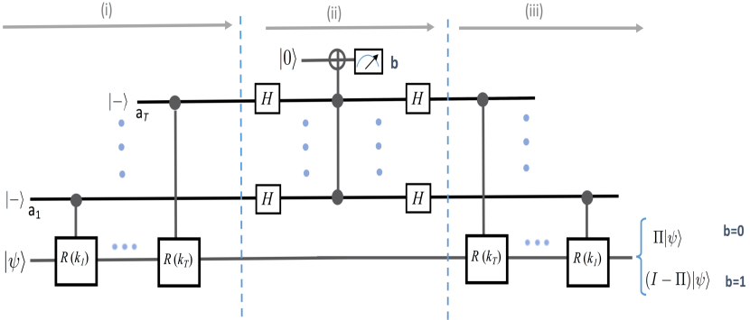
Figure 3: The circuit for emulating the two-outcome projective measurement with projectors $\{\Pi,I-\Pi\}$, where $\Pi$ is the projector to the subspace spanned by the sample states $\{|\phi_{k}\rangle:1,\cdots,K\}$.

E.0.1 The Algorithm

The quantum circuit for this algorithm is presented in Fig.(3). The algorithm has the following three steps:

(i) Consider $T$ qubits $a_{1}\cdots a_{T}$, which are all initially prepared in state $|-\rangle=(|0\rangle-|1\rangle)/\sqrt{2}$. Let $k_{1},\cdots,k_{T}$ be $T$ independent random integers, each chosen uniformly at random form $1,\cdots,K$. Apply the controlled-reflection $R_{a_{1}}(k_{1})$ to the system and qubit $a_{1}$, $R_{a_{2}}(k_{2})$ to the system and qubit $a_{2}$, until the last controlled-reflection $R_{a_{T}}(k_{T})$, which is applied to the system and qubit $a_{T}$.

(ii) Perform the two-outcome projective measurement $\{|-\rangle\langle-|^{\otimes T},I-|-\rangle\langle-|^{\otimes T}\}$ on qubits $a_{1}\cdots a_{T}$. (This can be implemented efficiently, e.g., by first applying the Hadamard gates on qubits $a_{1}\cdots a_{T}$, then applying a $T$-bit Toffoli gate controlled by $a_{1}\cdots a_{T}$, that is acting on an ancillary qubit initialized in state $|0\rangle$, and finally applying the Hadamard gates on qubits $a_{1}\cdots a_{T}$ again. Then, measuring this ancillary qubit in the computational basis, realizes the desired measurement.)

(iii) Recall the random integers $k_{1},\cdots,k_{T}$ chosen in step (i). Apply the controlled-reflection $R_{a_{T}}(k_{T})$ to the system and qubit $a_{T}$, then apply the controlled-reflection $R_{a_{T-1}}(k_{T-1})$ to the system and qubit $a_{T-1}$, until the last controlled-reflection $R_{a_{1}}(k_{1})$ which is applies to the system and qubit $a_{1}$.

Then, at the end of the algorithm, the initial state $|\psi\rangle$ is projected to state $\Pi|\psi\rangle/\sqrt{\langle\psi|\Pi|\psi\rangle}$ with probability $\langle\psi|\Pi|\psi\rangle$ (corresponding to outcome $b=0$ in the measurement in step (ii)), and is projected to state $(I-\Pi)|\psi\rangle/\sqrt{1-\langle\psi|\Pi|\psi\rangle}$ with probability $1-\langle\psi|\Pi|\psi\rangle$ (corresponding to outcome $b=1$ in the measurement).

E.0.2 How it works

In the following we assume the circuit is run with perfect controlled-reflections. Then, the additional error due to the imperfections in the simulations of the controlled-reflections can be taken into account, using the same approach we used for the main algorithm.

Let $\mathcal{E}$ be the quantum channel that describes the overall effect of circuit in Fig.(3) in the case where we ignore the output of measurement, i.e. we do not postselect. Let $\mathcal{H}_{\Pi}$ be the subspace spanned by the sample states $\{|\phi_{k}\rangle:k=1,\cdots,K\}$.

Theorem 4

Let $\lambda_{\text{min}}$ be the minimum non-zero eigenvalue of the density operator $K^{-1}\sum_{k=1}^{K}|\phi_{k}\rangle\langle\phi_{k}|$. If the support of $\rho$, the state of system is contained in either the subspace $\mathcal{H}_{\Pi}$ or the orthogonal subspace, then the probability of error in emulating the measurement $\{I-\Pi,\Pi\}$ is less than or equal to $(1-\lambda_{\text{min}})^{T}$. Furthermore, the fidelity of $\mathcal{E}(\rho)$, the output of the circuit, with $\rho$ the desired output state, satisfies $F(\mathcal{E}(\rho),\rho)\geq 1-(1-\lambda_{\text{min}})^{T}$.

Proof. First, consider the case where $\rho$, the initial state of system, does not have any support on $\mathcal{H}_{\Pi}$, i.e. $\Pi\rho\Pi=0$. Then, all the reflections $e^{i\pi|\phi_{k}\rangle\langle\phi_{k}|}$ act as the identity operator on this state. Therefore, after step (i) the state of qubits $a_{1}\cdots a_{T}$ remain unchanged. In this case, in step (ii) with probability one we project these qubits to state $|-\rangle^{\otimes T}$. It follows that in this case the algorithm emulates the action of measurement perfectly.

Next, we consider the case where $\Pi\rho\Pi=\rho$. Using the fact that

$$\langle-|R_{a}(k)|-\rangle_{a}=\frac{I+e^{i\pi|\phi_{k}\rangle\langle\phi_{k}|}}{2}=I-|\phi_{k}\rangle\langle\phi_{k}|\ ,$$ (82)

we find that for a general state $\rho$ (not necessarily restricted to $\mathcal{H}_{\Pi}$) the probability that in step (ii) we find the qubits $a_{1}\cdots a_{T}$ in state $|-\rangle^{\otimes T}$ is given by

$$p(|-\rangle^{\otimes T}) =\frac{1}{K^{T}}\sum_{k_{1},\cdots,K_{T}}^{K}\textrm{Tr}\Big{(}[|-\rangle\langle-|^{\otimes T}\otimes I]\ R_{a_{T}}(k_{T})\cdots R_{a_{1}}(k_{1})\ \left[\rho\otimes|-\rangle\langle-|^{\otimes T}\right]\ R_{a_{1}}(k_{1})\cdots R_{a_{T}}(k_{T})\Big{)}$$ (83a)

$$=\frac{1}{K^{T}}\sum_{k_{1},\cdots,K_{T}}^{K}\textrm{Tr}\Big{(}(I-|\phi_{k_{T}}\rangle\langle\phi_{k_{T}}|)\cdots(I-|\phi_{k_{1}}\rangle\langle\phi_{k_{1}}|)\ \rho\ (I-|\phi_{k_{1}}\rangle\langle\phi_{k_{1}}|)\cdots(I-|\phi_{k_{T}}\rangle\langle\phi_{k_{T}}|)\Big{)}$$ (83b)

$$=\textrm{Tr}\left(\mathcal{M}^{T}(\rho)\right)\ ,$$ (83c)

where $\mathcal{M}(\cdot)=\frac{1}{K}\sum_{k=1}^{K}P_{k}^{\perp}(\cdot)P_{k}^{\perp}\ ,$ and $P_{k}^{\perp}=I-|\phi_{k}\rangle\langle\phi_{k}|$.

Next, note that for any operator $X$ we have

$$\textrm{Tr}(\mathcal{M}(X))=\frac{1}{K}\sum_{k=1}^{K}\textrm{Tr}(XP_{k}^{\perp})=\textrm{Tr}(X)-\textrm{Tr}\Big{(}X\sum_{k=1}^{K}\frac{1}{K}|\phi_{k}\rangle\langle\phi_{k}|\Big{)}=\textrm{Tr}(X)-\textrm{Tr}(X\sigma_{\text{avg}})\ ,$$ (84)

where

$$\sigma_{\text{avg}}\equiv\frac{1}{K}\sum_{K}|\phi_{k}\rangle\langle\phi_{k}|\ .$$ (85)

The subspace $\mathcal{H}_{\Pi}$ is defined as the subspace spanned by $\{|\phi_{k}\rangle:k=1,\cdots,K\}$. Therefore, the density matrix $\sigma_{\text{avg}}$ is automatically full-rank in this subspace. Let $\lambda_{\text{min}}$ be the minimum eigenvalue of $\sigma_{\text{avg}}$ in this subspace, i.e. the minimum nonzero eigenvalue of $\sigma_{\text{avg}}$. Note that for any positive operator $X$ whose support is restricted to $\mathcal{H}_{\Pi}$ we have

$$\textrm{Tr}(X\sigma_{\text{avg}})\geq\lambda_{\text{min}}\textrm{Tr}(X)\ .$$ (86)

Then, using Eq.(84) this means that for any positive operator $X$, whose support is restricted to $\mathcal{H}_{\Pi}$ we have

$$\textrm{Tr}(\mathcal{M}(X))=\textrm{Tr}(X)-\textrm{Tr}(X\sigma_{\text{avg}})\leq\textrm{Tr}(X)(1-\lambda_{\text{min}})\ .$$ (87)

Next, note that if $X$ is a positive operator with support restricted to $\mathcal{H}_{\Pi}$, then $\mathcal{M}(X)$ is also a positive operator with support restricted to $\mathcal{H}_{\Pi}$. It follows that if $X$ is a positive operator with support restricted to $\mathcal{H}_{\Pi}$, then

$$\textrm{Tr}(\mathcal{M}^{T}(X))\leq\textrm{Tr}(X)\times(1-\lambda_{\text{min}})^{T}\ .$$ (88)

This together with Eq.(83) imply that if the support of the initial state $\rho$ is restricted to $\mathcal{H}_{\Pi}$, then the probability that at the end of algorithm we find qubits $a_{1}\cdots a_{T}$ in state $|-\rangle^{\otimes T}$ is given by

$$p(|-\rangle^{\otimes T})=\textrm{Tr}\left(\mathcal{M}^{T}(\rho)\right)\leq(1-\lambda_{\text{min}})^{T}\ .$$ (89)

This completes the proof of the first part of the theorem.

Finally, the second part of the theorem, i.e. the bound on the fidelity, follows from the following lemma, which is proven in the same way we proved Theorem 1.

Lemma 5

Consider the following quantum operation: (i) We apply a unitary $V(\boldsymbol{\lambda})$ to the system, where $\boldsymbol{\lambda}$ is a random parameter chosen according to the probability distribution $p(\boldsymbol{\lambda})$. (ii) We perform a projective measurement on the system with projectors $\{P_{\alpha}:\alpha\in A\}$. (iii) We apply the unitary $V^{\dagger}(\boldsymbol{\lambda})$.

Let $\mathcal{G}$ be the quantum channel that describes the overall effect of this operation on the system, in the case where we ignore the outcome of the projective measurement. Then, for any input state $\rho$, the fidelity of $\rho$ and $\mathcal{G}(\rho)$ satisfies

$$F(\rho,\mathcal{G}(\rho))\geq\underset{\alpha\in A}{\textrm{max}}\ p_{\alpha}(\rho)$$ (90)

where $p_{\alpha}(\rho)$ is the (average) probability of outcome $\alpha$ in the measurement.

Proof. Quantum operation $\mathcal{G}$ is given by

$$\mathcal{G}(\cdot)=\sum_{\boldsymbol{\lambda}}p(\boldsymbol{\lambda})\sum_{\alpha\in A}V^{\dagger}(\boldsymbol{\lambda})P_{\alpha}V(\boldsymbol{\lambda})(\cdot)V^{\dagger}(\boldsymbol{\lambda})P_{\alpha}V(\boldsymbol{\lambda})\ .$$ (91)

Consider a pure input state $|\gamma\rangle$. Then, the squared fidelity of $\mathcal{G}(|\gamma\rangle\langle\gamma|)$ and $|\gamma\rangle\langle\gamma|$ is given by

$$F^{2}(\mathcal{G}(|\gamma\rangle\langle\gamma|),|\gamma\rangle\langle\gamma|) =\langle\gamma|\mathcal{G}(|\gamma\rangle\langle\gamma|)|\gamma\rangle$$ (92)

$$=\sum_{\alpha\in A}\sum_{\boldsymbol{\lambda}}p(\boldsymbol{\lambda})\langle\gamma|V^{\dagger}(\boldsymbol{\lambda})P_{\alpha}V(\boldsymbol{\lambda})|\gamma\rangle^{2}$$ (93)

$$\geq\underset{\alpha\in A}{\textrm{max}}\ \sum_{\boldsymbol{\lambda}}p(\boldsymbol{\lambda})\langle\gamma|V^{\dagger}(\boldsymbol{\lambda})P_{\alpha}V(\boldsymbol{\lambda})|\gamma\rangle^{2}$$ (94)

$$\geq\underset{\alpha\in A}{\textrm{max}}\ \Big{(}\sum_{\boldsymbol{\lambda}}p(\boldsymbol{\lambda})\langle\gamma|V^{\dagger}(\boldsymbol{\lambda})P_{\alpha}V(\boldsymbol{\lambda})|\gamma\rangle\Big{)}^{2}$$ (95)

$$=\underset{\alpha\in A}{\textrm{max}}\ p_{\alpha}^{2}(|\gamma\rangle\langle\gamma|)\ ,$$ (96)

where to get the fourth line we have used the fact that the variance of any random variable is non-negative, and to get the last line we have used the fact that the average density operator of the system before the measurement is $\sum_{\boldsymbol{\lambda}}p(\boldsymbol{\lambda})V(\boldsymbol{\lambda})|\gamma\rangle\langle\gamma|V^{\dagger}(\boldsymbol{\lambda})$, and so the probability of outcome $\alpha$ is $\sum_{\boldsymbol{\lambda}}p(\boldsymbol{\lambda})\langle\gamma|V^{\dagger}(\boldsymbol{\lambda})P_{\alpha}V(\boldsymbol{\lambda})|\gamma\rangle$. This proves the lemma for the special case of pure states. The result for general mixed states follows from the joint concavity of fidelity.   

This lemma together with the fact that for input states contained in $\mathcal{H}_{\Pi}$, or the complement subspace the outcome of the ideal measurement is deterministic, and the circuit generates this outcome with probability of error less than $(1-\lambda_{\text{min}})^{T}$, proves the bound

$$F(\mathcal{E}(\rho),\rho)\geq 1-(1-\lambda_{\text{min}})^{T}\ .$$ (97)

This completes the proof of theorem.

References

• S. Lloyd (1996) S. Lloyd, Science 273, 1073 (1996).
• Bisio etΒ al. (2010) A.Β Bisio, G.Β Chiribella, G.Β M. D’Ariano, S.Β Facchini, and P.Β Perinotti, Physical Review A 81, 032324 (2010).
• Lloyd etΒ al. (2014) S.Β Lloyd, M.Β Mohseni, and P.Β Rebentrost, Nature Physics 10, 631 (2014).
• Nielsen and Chuang (2000) M.Β Nielsen and I.Β Chuang, Quantum Computation and Quantum Information, Cambridge Series on Information and the Natural Sciences (Cambridge University Press, 2000), ISBN 9780521635035.
• Uhlmann (1976) A.Β Uhlmann, Reports on Mathematical Physics 9, 273 (1976).
• Jozsa (1994) R.Β Jozsa, Journal of modern optics 41, 2315 (1994).
• Wootters and Zurek (1982) W.Β K. Wootters and W.Β H. Zurek, Nature 299, 802 (1982).
• Bartlett etΒ al. (2007) S.Β D. Bartlett, T.Β Rudolph, and R.Β W. Spekkens, Reviews of Modern Physics 79, 555 (2007).
• Marvian and Spekkens (2013) I.Β Marvian and R.Β W. Spekkens, New Journal of Physics 15, 033001 (2013).
• Marvian and Spekkens (2014) I.Β Marvian and R.Β W. Spekkens, Phys. Rev. A 90, 062110 (2014), URL http://link.aps.org/doi/10.1103/PhysRevA.90.062110.
• Gour and Spekkens (2008) G.Β Gour and R.Β W. Spekkens, New Journal of Physics 10, 033023 (2008).
• Marvian and Mann (2008) I.Β Marvian and R.Β Mann, Physical Review A 78, 022304 (2008).
• Cirac etΒ al. (1999) J.Β Cirac, A.Β Ekert, and C.Β Macchiavello, Physical review letters 82, 4344 (1999).
Supplementary Material