Minimum Restraint Functions
for unbounded dynamics:
general and control-polynomial systems

Abstract.

We consider an exit-time minimum problem with a running cost   $l\geq 0$ and unbounded controls. The occurrence of points where $l=0$ can be regarded as a transversality loss. Furthermore, since controls range over unbounded sets, the family of admissible trajectories may lack important compactness properties. In the first part of the paper we show that the existence of a ${p_{0}}$-Minimum Restraint Function provides not only global asymptotic controllability (despite non-transversality) but also a state-dependent upper bound for the value function (provided $p_{0}>0$). This extends to unbounded dynamics a former result which heavily relied on the compactness of the control set.

In the second part of the paper we apply the general result to the case when the system is polynomial in the control variable. Some elementary, algebraic, properties of the convex hull of vector-valued polynomials’ ranges allow some simplifications of the main result, in terms of either near-affine-control systems or reduction to weak subsystems for the original dynamics.

1. Introduction

Mainly motivated by the case when the dynamics is polynomial in the control, we deal with optimal control problems of the form

(1.1) $$\dot{x}=f(x,u),\qquad x(0)=z,$$

(1.2) $$(x(t),u(t))\in(\Omega\backslash{\bf C})\times U,\quad\lim_{t\to{T}_{x}^{-}}{\bf d}(x(t),\mathbf{C})=0,$$

(1.3) $$\displaystyle{{\mathcal{I}}(x,u):=\int_{0}^{T_{x}}l(x(t),u(t))\,dt,}\qquad\displaystyle{V(z):=\inf_{(x,u)}{\mathcal{I}}(x,u)},$$

where: i) for given positive integers $n,m$, the state space $\Omega$ is an open subset of ${I\!\!R}^{n}$, the controls $u$ range over a (possibly unbounded) subset of $U\subseteq{I\!\!R}^{m}$, and ${\bf C}\subset\Omega$ is a closed target with compact boundary; ii) the current cost $l(x,u)$ is $\geq 0$ for all $(x,u)\in(\Omega\backslash{\bf C})\times U$; iii) $T_{{x}}\in[0,+\infty]$ is the infimum of times needed for the trajectory $x(\cdot)$ to approach the target $\mathbf{C}$; and iv) $\mathbf{d}(x,{\bf C})$ denotes the usual (Euclidean) distance of the point $x$ from the subeset $\bf C$.

We focus on a particular kind of Lyapunov function, called $p_{0}$-Minimum Restraint Function (${p_{0}}\geq 0$). This notion has been introduced in [14] under the extra-hypothesis that the controls range over a bounded set. The existence of a $p_{0}$-Minimum Restraint Function, besides implying global asymptotic controllability to $\mathbf{C}$, was shown to provide a continuous upper estimate for the value function $V$. Such an estimate is not trivial, in that the problem (here and in [14] as well) lacks what in first order PDE’s is called transversality, which would correspond to the assumption $l(x,u)\neq 0$ for all $(x,u)$ (as in the minimal time problem, where $l=1$). Here, we extend the concept of $p_{0}$-Minimum Restraint Function to unbounded dynamics $f$. Notice that the unboundedness of $f$ (and $l$) cannnot be neglected, for no coercivity hypotheses –roughly speaking, the fact that $u\mapsto l(x,u)$ grows suitably faster than $u\mapsto f(x,u)$ – rule out the need of larger and larger velocities in a minimizing sequence.

Precisely, for a ${p_{0}}\geq 0$ we call ${p_{0}}$-Minimum Restraint Function every continuous function

$$W:\Omega\setminus\overset{\circ}{\mathbf{C}}\to[0,+\infty[$$

whose restriction to $\Omega\setminus\mathbf{C}$ (is locally semiconcave, positive definite and proper , and) verifies

(1.4) $$H_{l,f}(x,{p_{0}},D^{*}W(x))<0\quad\forall x\in\Omega\setminus\mathbf{C},$$

where the Hamiltonian $H_{l,{f}}$ is defined by

(1.5) $$H_{l,f}(x,p_{0},p):=\inf_{u\in U}\Big{\{}\langle p,f(x,u)\rangle+p_{0}\,l(x,u)\Big{\}}.$$

The inequality (1.4) has to be interpreted as $H_{l,{f}}(x,{p_{0}},p)<0$ $\forall p\in D^{*}W(x)$—which includes the case $H_{l,{f}}(x,{p_{0}},p)=-\infty$ . The following hypothesis will be crucial: Hypothesis A: For every compact subset ${\mathcal{K}}\subset\Omega\backslash\mathbf{C}$ the function

(1.6) $$(\bar{l},\bar{{f}})(x,u):=\frac{(l,{{f}})}{1+|(l,{f})(x,u)|}(x,u)$$

is uniformly continuous on ${\mathcal{K}}\times U$.

Observe that Hypothesis A allows for a vast class of cost-dynamic pairs $(l,f)(x,u)$, including ($x$-dependent) polynomials in $u_{1},\cdots,u_{m}$, $|u_{1}|,\cdots,|u_{m}|$, $|u|$, and compositions of polynomials with exponential and Lipschitz continuous functions. Let us bring forward the statement of our main result:

Theorem 1.1.

Assume Hypothesis A and let $W$ be a ${p_{0}}$-Minimum Restraint Function for the problem $(l,f,\mathbf{C})$, for some ${p_{0}}\geq 0$. Then

• system (1.1) is globally asymptotically controllable to $\mathbf{C}$.

Furthermore,

• if ${p_{0}}>0$, then

  (1.7) $${{V}}(z)\leq\frac{W(z)}{{{{p_{0}}}}}\,\qquad\forall z\in\Omega\setminus\mathbf{C}.$$

The proof of the theorem relies on a state-based time rescaling of the problem, which in turn is made possible by Hypothesis A. The controls of the rescaled problem (see Section 2) still range in the (possibly unbounded) set $U$. Yet, some compactness properties of the rescaled dynamics are of crucial importance in the construction of trajectories reaching the target at least asymptotically.

An application to the gyroscope (see Subsection 2.2) concludes Section 2: an explicit ${p_{0}}$-Minimum Restraint Function is provided for a minimum problem where the control is identified with the pair made by the precession and spin velocities, while the state corresponds to pair made by the nutation angle and its time-derivative.

The remaining part of the paper is devoted to problems whose dynamics can be parameterized by a $u$-polynomial:

(1.8) $$\dot{x}=\displaystyle f(x,u):=f_{0}(x)+\sum_{i=1}^{d}\left(\sum_{\alpha\in{\mathbb{N}}^{m},\,\alpha_{1}+\dots+\alpha_{m}=i}u_{1}^{\alpha_{1}}\cdots u_{m}^{\alpha_{m}}f_{\alpha_{1},\dots,\alpha_{m}}(x)\right)\,.$$

Among applications for which the polynomial dependence is relevant let us mention Lagrangian mechanical systems, possibly with friction forces, in which inputs are identified with the derivatives of some Lagrangian coordinates. In this case $d=2$. We point out also that, in connection with the investigation of uniqueness and regularity of solutions for Hamilton-Jacobi equations, dynamics and current costs with unbounded controls and polynomial growth have been already addressed in [13], [15], by embedding the problem in a space-time problem through techniques of graph’s reparameterization – see e.g. [3, 4, 5, 9, 12, 19, 18, 21]. With similar arguments (see also [11]) necessary conditions for the existence of (possibly impulsive) minima of input-polynomial optimal control problems have been studied in [8]. Furthermore, the interplay between convexity and polynomial dependence of both the dynamics and the running cost   has been investigated also in [17], in connection with problems of existence of optimal solutions.

A careful investigation of elementary, algebraic properties of the convex hull $co~{}f(x,{I\!\!R}^{m})$ proves essential for the application of Theorem 1.1 to the polynomial case (1.8). For instance, we consider near-control-affine control systems, a class of control-polynomial systems where the convex hull of the dynamics can be parameterized as a control-affine system with controls in a neighborhood of the origin. For instance, this is clearly false for the system $\dot{x}=f_{0}(x)+uf_{1}(x)+u^{2}f_{2}(x),$ $u\in{I\!\!R},$ – because the origin $(0,0)$ does not belong to the the convex hull’s interior of the curve $(u,u^{2})$. Instead, in view of Theorem 4.3, the convex hull of the image of

$$f_{0}(x)+u_{1}f_{1,0,0,0,0,0,0}(x)+u_{1}u^{5}_{3}f_{1,0,5,0,0,0,0}(x)+u_{2}^{3}u_{6}^{3}f_{0,3,0,0,0,3,0}(x)\\ +u_{1}u_{3}^{5}u_{7}^{9}f_{1,0,5,0,0,0,9}(x),$$

$(u_{1},\dots,u_{7})\in{I\!\!R}^{7}$ does coincide with the range of

$$f_{0}(x)+w_{1}f_{1,0,0,0,0,0,0}(x)+w_{2}f_{1,0,5,0,0,0,0}(x)+w_{3}f_{0,3,0,0,0,3,0}(x)+w_{4}f_{1,0,5,0,0,0,9}(x),$$

$(w_{1},w_{2},w_{3},w_{4})\in{I\!\!R}^{4}.$

When the system is not near-control-affine (and $U={I\!\!R}^{m}$), one can try to exploit weak subsystems: the latter are selections of the set-valued function $x\mapsto co~{}f(x,{I\!\!R}^{m})$. In particular, we consider the maximal degree subsystem and, for any $\lambda$ in the $m$-dimensional simplex, the $\lambda$-diagonal subsystems (see Definition 4.9 and Subsection 4.2, respectively). The idea of utilizing subsystems might look counterproductive with respect to the task of finding a ${p_{0}}$-Minimum Restraint Function: indeed, for such a purpose, having a sufficiently large amount of available directions plays crucial. However, from a practical perspective, a diminished complexity in the dynamics might ease the guess of a ${p_{0}}$-Minimum Restraint Function, which would automatically be a ${p_{0}}$-Minimum Restraint Function for the original polynomial problem. To give the flavour of this viewpoint, let us anticipate a result (see Theorem 4.7 for details) concerning maximal degree subsystems.

Theorem 1.2.

Let the growth assumption specified in Hypothesis A_max below (Section 4.2) be verified. If $W$ is a ${p_{0}}$-Minimum Restraint Function for the maximal degree subsystem

$$f^{max}(x,u):=f_{0}(x)+\sum_{\alpha\in{\mathbb{N}}^{m},\,\alpha_{1}+\dots+\alpha_{m}=d}u_{1}^{\alpha_{1}}\cdots u_{m}^{\alpha_{m}}f_{\alpha_{1}\dots\alpha_{m}}(x),$$

then $W$ is also a ${p_{0}}$-Minimum Restraint Function for the original control polynomial system

$$f(x,u):=f_{0}(x)+\sum_{i=1}^{d}\left(\sum_{\alpha\in{\mathbb{N}}^{m},\,\alpha_{1}+\dots+\alpha_{m}=i}u_{1}^{\alpha_{1}}\cdots u_{m}^{\alpha_{m}}f_{\alpha_{1},\dots,\alpha_{m}}(x)\right)\,.$$

The paper is organized as follows. In the remaining part of the present section we provide some preliminary definitions and notation. In Section 2 we prove Theorem 1.1 and exhibit a ${p_{0}}$-Minimum Restraint Function for the gyroscope (see Subsection 2.2). Section 3 is entirely devoted to the proof of Theorem 3.1 which deals with a suitably rescaled problem. In Section 4 we focus on the case when the system is polynomial in the control variable. An Appendix with a technical proof concludes the paper.

1.1. Preliminary concepts and notation

  Let us gather some notational conventions as well as some basic concepts and results which will be used throughout the paper.

We are given an open set $\Omega\subset{I\!\!R}^{n}$ and a target $\mathbf{C}\subset\Omega$, which we assume to have compact boundary $\partial\mathbf{C}$. For brevity, let us use the notation ${\bf d}(x)$ in place of ${\bf d}(x,\mathbf{C})$.

Definition 1.3.

We say that a path $x:[0,T_{x}[\to\Omega$ is admissible if

• $0<T_{x}\leq+\infty$,

• $x\in AC_{loc}([0,T_{x}[,\Omega)$,

• $x([0,T_{x}[)\subset\Omega\backslash\mathbf{C}$,

• $\displaystyle\lim_{t\to T^{-}_{x}}{\bf d}(x(t))=0$.

We call $T_{x}$ the exit time of $x$ from $\Omega\setminus\mathbf{C}$.

Notice that the limit of $x(\cdot)$ for $t\to T_{x}^{-}$ need not exist, even when $T_{x}<+\infty$. Of course, if the limit exists, then it belongs to the target $\mathbf{C}$.

Definition 1.4.

Let $g:\Omega\times U\to{I\!\!R}^{n}$ be a continuous function. For every $z\in\Omega\setminus\mathbf{C}$, we will say that $(x,u)$ is an admissible trajectory-control pair from $z$ for the control system

(1.9) $$\dot{x}=g(x,u),\quad x(0)=z$$

if

• $x:[0,T_{x}[\to\Omega\setminus\mathbf{C}$ is an admissible path,

• $u(\cdot)\in L^{\infty}_{loc}([0,T_{x}[,U)$,

• $x(\cdot)$ is a Charathéodory solution of (1.9) corresponding to the input $u$.

We shall use ${\mathcal{A}}_{g}({z})$ to denote the family of admissible trajectory-control pairs from $z$ for the control system (1.9).

As customary, we shall use ${\mathcal{K}L}$ to denote the set of all continuous functions

$$\beta:[0,+\infty[\times[0,+\infty[\to[0,+\infty[$$

such that: (1)  $\beta(0,t)=0$ and $\beta(\cdot,t)$ is strictly increasing and unbounded for each $t\geq 0$; (2)  $\beta(r,\cdot)$ is decreasing for each $r\geq 0$; (3)  $\beta(r,t)\to 0$ as $t\to+\infty$ for each $r\geq 0$.

Definition 1.5.

The system (1.9) is globally asymptotically controllable to $\mathbf{C}$ – shortly, (1.9) is GAC to $\mathbf{C}$ – provided there is a function $\beta\in{\mathcal{K}L}$ such that, for each initial state $z\in\Omega\setminus\mathbf{C}$, there exists an admissible trajectory-control pair $(x,u)\in{\mathcal{A}}_{g}({z})$ that verifies

(1.10) $${\bf d}(x(t))\leq\beta({\bf d}(z),t)\qquad\forall t\in[0,+\infty[.\,\,$$

Definition 1.6 (Positive definite and proper functions).

Let ${\bf E}$, $\Theta\subset{I\!\!R}^{n}$ be, respectively, a closed and an open set with ${\bf E}\subset\Theta$ and let $F:\Theta\setminus\overset{\circ}{\bf E}\to{I\!\!R}$ be a continuous function. Then $F$ is positive definite on $\Theta\setminus{\bf E}$ if $F(x)>0$ for all $x\in\Theta\setminus{\bf E}$ and $F(x)=0$ for all $x\in\partial{\bf E}$.
The function $F$ is called proper on $\Theta\setminus{\bf E}$ if the pre-image $F^{-1}(K)$ of any compact set $K\subset[0,+\infty)$ is compact.

Definition 1.7 (Semiconcave functions).

Let $\Theta\subseteq{I\!\!R}^{n}$. A continuous function $F:\Theta\to{I\!\!R}$ is said to be semiconcave on $\Theta$ if

$$F(z_{1})+F(z_{2})-2F\left(\frac{z_{1}+z_{2}}{2}\right)\leq\rho|z_{1}-z_{2}|^{2},$$

for all $z_{1}$, $z_{2}\in\Theta$ such that $[z_{1},z_{2}]\subseteq\Theta$. $F$ is said to be locally semiconcave on $\Theta$ if it semiconcave on every compact subset of $\Theta$.

We remind that locally semiconcave functions are locally Lipschitz continuous.

Definition 1.8 (Limiting gradient).

Let $\Theta\subset{I\!\!R}^{n}$ be an open set and let $F:\Theta\to{I\!\!R}$ be a locally Lipschitz function. For every $x\in\Theta$ we set

$$D^{*}{F}(x):=\Big{\{}w\in{I\!\!R}^{n}\mid\ \ w=\lim_{k}\nabla{F}(x_{k}),\ \ x_{k}\in DIFF(F)\setminus\{x\},\ \ \lim_{k}x_{k}=x\Big{\}}$$

where $\nabla$ denotes the classical gradient operator and $DIFF(F)$ is the set of differentiability points of $F$. $D^{*}{F}(x)$ is called the set of limiting gradients of $F$ at $x$.

Remark 1.9.

The set-valued map $x\mapsto D^{*}F(x)$ is upper semicontinuous on $\Theta$, with non-empty, compact values. Notice that $D^{*}{F}(x)$ is not convex. When $F$ is a locally semiconcave function, $D^{*}{F}$ coincides with the limiting subdifferential $\partial_{L}F$, namely,

$$D^{*}F(x)=\partial_{L}F(x):=\{\lim\,p_{i}:\ p_{i}\in\partial_{P}F(x_{i}),\ \lim\,x_{i}=x\}\quad\forall x\in\Theta,$$

where $\partial_{P}F$ denotes the proximal subdifferential, largely used in the literature on Lyapunov functions.

Basic properties of the semiconcave functions imply the following fact:

Lemma 1.10.

Let $\Theta\subset{I\!\!R}^{n}$ be an open set and let $F:\Theta\to{I\!\!R}$ be a locally semiconcave function. Then for any compact set $\mathcal{K}\subset\Theta$ there exist some positive constants $L$ and $\rho$ such that, for any $x\in\mathcal{K}$ ,

(1.11) $$\begin{array}[]{l}F(\hat{x})-F(x)\leq\langle p,\hat{x}-x\rangle+\rho|\hat{x}-x|^{2},\\ \\ |p|\leq L\quad\forall p\in D^{*}F(x),\end{array}$$

for any point $\hat{x}\in\mathcal{K}$ such that $[x,\hat{x}]\subset\mathcal{K}$.

2. ${p_{0}}$-Minimum restraint functions

2.1. The main result

  Let us begin with a precise formulation of the minimum problem. For every initial condition $z\in\Omega\setminus\mathbf{C}$, we consider the control system

(2.1) $$\dot{x}=f(x,u),\quad x(0)=z,$$

and, for any admissible trajectory-control pair $(x,u)\in{\mathcal{A}}_{f}(z)$ (see Definition 1.4), let us introduce the payoff

(2.2) $${\mathcal{I}}(x,u):=\int_{0}^{T_{x}}l(x(t),u(t))\,dt\qquad(T\in]0,+\infty]).$$

The corresponding value function is given by

(2.3) $$V(z)\>=\inf_{(x,u)\in{\mathcal{A}}_{f}({z})}{\mathcal{I}}(x,u)\quad(\leq+\infty).$$

Recall our principal hypothesis:

Hypothesis A: For every compact subset ${\mathcal{K}}\subset\Omega\backslash\mathbf{C}$ the function

(2.4) $$(\bar{l},\bar{{f}})(x,u):=\frac{(l,{{f}})}{1+|(l,{f})(x,u)|}(x,u)$$

is uniformly continuous on ${\mathcal{K}}\times U$.

Remark 2.1.

As observed in the Introduction, this hypothesis allows for a wide set of unbounded dynamics and running costs. Furthermore, it is easy to check that the following condition is sufficient for Hypothesis A to hold true:

 

• The map  $(l,{f})$ is continuous with respect to the state variable $x$ and locally Lipschitz with respect to the control variable $u$, and

  $$\left|\frac{D_{u}(l,{f})}{(1+|(l,{f})|)^{2}}\right|(x,u)\leq\eta(x)\qquad\text{ for a.e. }(x,u)\in(\Omega\backslash\mathbf{C})\times U,$$

  for some continuous function $\eta:~{}\Omega\backslash\mathbf{C}\to~{}[0,+\infty[$.

Let us extend the definition of ${p_{0}}$-Minimum Restraint Function ([14]) to the case of unbounded control sets.

Definition 2.2.

Let $W:\Omega\setminus\overset{\circ}{\mathbf{C}}\to[0,+\infty[$ be a continuous function, and let us assume that $W$ is locally semiconcave, positive definite, and proper on $\Omega\setminus\mathbf{C}$. We say that $W$ is a $p_{0}$-Minimum Restraint Function –in short, ${p_{0}}$-MRF– for $(l,{f},\mathbf{C})$ in $\Omega$ for some ${p_{0}}\geq 0$ if

(2.5) $$H_{l,{f}}(x,{p_{0}},D^{*}W(x))<0\quad\forall x\in{{\Omega}\setminus\mathbf{C}}\quad$$

and, moreover, there exists $W_{0}\in[0,+\infty]$, such that

$$W(\Omega\setminus{\mathbf{C}})<W_{0}\quad\text{and}\quad\lim_{x\to x_{0},\ x\in\Omega}W(x)=W_{0}$$

for every $x_{0}\in\partial\Omega$.

We can now state our main result: Theorem 1.1. Assume Hypothesis A and let $W$ be a ${p_{0}}$-Minimum Restraint Function for the problem $(l,f,\mathbf{C})$, for some ${p_{0}}\geq 0$. Then:

• system (2.1) is globally asymptotically controllable to $\mathbf{C}$;

• if ${p_{0}}>0$, then

  (2.6) $${{V}}(z)\leq\frac{W(z)}{{{{p_{0}}}}}\,\qquad\forall z\in\Omega\setminus\mathbf{C}.$$

Proof.

We begin with a state-based rescaling procedure. Precisely, we consider the optimal control problem

(2.7) $$\begin{array}[]{l}\displaystyle y^{\prime}(s)=\bar{f}(y,v)\quad y(0)=z;\\ \\ \displaystyle{\mathcal{I}}_{\bar{l},\bar{f}}(y,v):=\int_{0}^{S_{y}}\bar{l}(y(s),v(s))ds,\qquad\bar{V}(z):=\displaystyle\inf_{(y,v)\in{\mathcal{A}}_{\bar{f}}({z})}{\mathcal{I}}_{\bar{l},\bar{f}}(y,v),\end{array}$$

where $\bar{l}$, $\bar{{f}}$ are defined in (2.4), the apex denotes differentiation with respect to the parameter $s$, and $S_{y}\leq+\infty$ is the exit time of the admissible trajectory $y(\cdot)$ (in the time parameter $s$).

The connection between the original optimal control problem and the rescaled one is established by the following result.

Claim 2.1.

The path $(y,v)$ is an admissible trajectory-control pair for (2.7) if and only if, setting

$$t(s):=\int_{0}^{s}(1+|(l,{f})(y(\eta),v(\eta)|)^{-1}d\eta\qquad\forall s\in[0,S_{y}[$$

$$x(t):=y\circ s(t)\qquad u(t):=v\circ s(t)\qquad\ \forall t\in[0,T_{x}[,\quad T_{x}:=t(S_{y}),$$

the path $(x,u)$ is an admissible trajectory-control pair for (2.1)–(2.3). Furthermore,

$$\int_{0}^{S_{y}}\bar{l}(y(s),v(s))ds=\displaystyle\int_{0}^{T_{x}}l(x(t),u(t))dt.$$

In particular, one has

$$V(z)=\bar{V}(z)$$

for all $z\in\Omega\setminus\mathbf{C}$.

Indeed, since $t=t(s)$ is absolutely continuous and $t^{\prime}(s)>0$ almost everywhere, the inverse map $s(\cdot)=t^{-1}(\cdot)$ is absolutely continuous (see e.g. [16, Theorem 4, page 253] or, for a more general statement, [7, Theorem 2.10.13, page 177]). In particular, $x=y\circ s$ is absolutely continuous, and $u=v\circ s$ turns out to be Borel measurable as well. Hence the claim follows by a standard application of the chain rule.

The Hamiltonian $H_{\bar{l},\bar{f}}$ associated to $\bar{l}$, $\bar{f}$,

$$H_{\bar{l},\bar{f}}(x,p_{0},p):=\inf_{u\in U}\Big{\{}\langle p,\bar{f}(x,u)\rangle+p_{0}\,\bar{l}(x,u)\Big{\}}$$

for all $(x,p_{0},p)\in(\Omega\backslash\mathbf{C})\times{I\!\!R}^{1+n},$ is continuous and sublinear in $(p_{0},p)$, uniformly with respect to $x$. Furthermore, it is also trivial to check that, for every $(x,p_{0},p)\in(\Omega\setminus\mathbf{C})\times{I\!\!R}^{1+n}$,

(2.8) $$H_{\bar{l},\bar{{f}}}(x,p_{0},p)<0\quad\iff\quad H_{l,{f}}(x,p_{0},p)<0.$$

In particular, for every ${p_{0}}\geq 0$ $W$ is a ${p_{0}}$-MRF for $(l,f,\mathbf{C})$ if and only if $W$ is a ${p_{0}}$-MRF for $(\bar{l},\bar{f},\mathbf{C})$. Moreover, because of Hypothesis A, the problem $(\bar{l},\bar{f},\mathbf{C})$ meets the hypotheses of Theorem 3.1 below. Therefore:

• if there exists a ${p_{0}}$-MRF $W$ for $(l,f,\mathbf{C})$, then the rescaled system in (2.7) is GAC to $\mathbf{C}$, i.e. there exists a function $\beta\in{\mathcal{K}\mathcal{L}}$ such that for any $z\in\Omega\setminus\mathbf{C}$ there is an admissible trajectory-control pair $(y,v)\in{\mathcal{A}}_{\bar{f}}(z)$ that verifies

  (2.9) $${\bf d}(y(s))\leq\beta({\bf d}(z),s)\qquad\forall s\in[0,+\infty[;$$

• moreover, if ${p_{0}}>0$, then

  (2.10) $${{\bar{V}}}(z)\leq\frac{W(z)}{{{{p_{0}}}}}.$$

If $x(\cdot)$ is the trajectory defined in Claim 2.1, one then obtains

(2.11) $${\bf d}(x(t))\leq\beta({\bf d}(z),s(t))\qquad\forall t\in[0,+\infty[$$

and, if ${p_{0}}>0$,

(2.12) $${{V}}(z)\leq\frac{W(z)}{{{{p_{0}}}}}\,\qquad\forall z\in\Omega\setminus\mathbf{C}.$$

Notice that $t(s)\leq s$ for all $s$, so that $t\leq s(t)$ for all $t$. Since the map $\beta(z,\cdot)$ is decreasing, one gets

$$\beta(z,s(t))\leq\beta(z,t)$$

for all $t$. It follows by (2.9) that

(2.13) $${\bf d}(x(t))\leq\beta({\bf d}(z),t)\qquad\forall t\in[0,+\infty[,$$

so the theorem is proved. ∎

We conclude this section with an application of Theorem 1.1 to Mechanics.

2.2. The gyroscope: controlling the nutation through precession and spin

  A gyroscope can be represented as a mechanism composed by a rotor –in our setting a spinning disk– and two gimbals. The spin axis of the rotor is fixed to the inner gimbal, whose spin axis is fixed to the outer gimbal (see Figure 1).

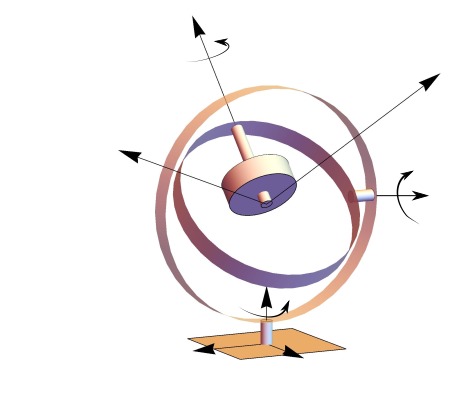
Figure 1.

Besides an inertial reference frame $OXYZ$ we consider a reference frame $oxyz$ fixed to the rotor. In particular, we choose the latter reference so that the centre of mass of the rotor has coordinates $(0,0,z_{G})$. The motion of the rotor can be parametrized by Euler angles as depicted in Figure 1: the outer gimbal’s position is represented by the precession angle $\phi$, the inner gimbal’s position is given by the nutation angle $\theta$, and the rotor’s position is measured by the spin angle $\psi$. The kinetic energy (in the inertial frame) is so given by

$${\mathcal{T}}=\frac{1}{2}I_{0}(\dot{\phi}^{2}\sin^{2}\theta+\dot{\theta}^{2})+\frac{1}{2}I(\dot{\phi}\cos\theta+\dot{\psi})^{2},$$

where $I_{0}$ is the moment of inertia of the rotor with respect to any axis through $o$ and orthogonal to $z$ and $I$ is the moment of inertia of the rotor about its spin axis $oz$. We have tacitly assumed that the rotor’s mass $M$ is the only non-negligible mass of the system. For simplicity, we also suppose $I_{0}=I$. If $g$ denotes the gravitational acceleration, the potential energy $\mathcal{V}$ is given by

$$\mathcal{V}(\theta):=Mgz_{G}\cos\theta\quad\forall\theta\in[-\pi/2,\pi/2].$$

We will regard the precession velocity $\dot{\phi}$ and the spin velocity $\dot{\psi}$ as controls belonging to $U={I\!\!R}^{2}$. Considering the predetermination of $\phi(\cdot)$ and $\psi(\cdot)$ as a holonomic constraint, we assume the classical D’Alembert hypothesis (see [2]).

The resulting control mechanical system is

(2.14) $$\begin{cases}\displaystyle{\dot{\theta}=\frac{1}{I}\pi_{\theta}}\\ \displaystyle{\dot{\pi}_{\theta}=Mgz_{G}\sin\theta-I\sin\theta\dot{\phi}\dot{\psi}},\end{cases}$$

where $\pi_{\theta}$ is the conjugate momentum $\pi_{\theta}:=\frac{\partial({\mathcal{T}}+\mathcal{V})}{\partial\dot{\theta}}=I\,\dot{\theta}$.

If we set $u:=(\dot{\phi},\dot{\psi})$, $x=(x_{1},x_{2})^{tr}:=(\theta,\pi_{\theta})$ , $f_{0}(x)=(I^{-1}x_{2},Mgz_{G}\sin x_{1})^{tr}$, and $f_{11}(x)=(0,-I\sin x_{1})^{tr}$ we obtain the control-quadratic control system

(2.15) $$\dot{x}=f(x,u):=f_{0}(x)+u_{1}u_{2}f_{11}(x),$$

with $(u_{1},u_{2})\in{I\!\!R}^{2}$. The state space of the control system (2.15) is the open set $\Omega=]-\pi/2,\pi/2[\times{I\!\!R}$ and we choose $\mathbf{C}=\{(0,0)\}$ as a target and $l(x_{1},x_{2})=x_{2}^{2}$ as a running cost  .

Let us set

$$W(x_{1},x_{2}):=W_{1}(x_{1},x_{2})(2-|W_{2}(x_{1},x_{2})|),$$

where

$$W_{1}(x_{1},x_{2}):=\tan^{2}x_{1}+x_{2}^{2},$$

$$W_{2}(x_{1},x_{2}):=\begin{cases}\sin\left(2\text{arctan}\left(\frac{-\tan x_{1}+\sqrt{3}x_{2}}{\sqrt{3}\tan x_{1}+x_{2}}\right)\right)&\text{ if }x_{2}\not=-\sqrt{3}\tan x_{1}\\ 0&\text{ otherwise }.\end{cases}$$

With some computation, one proves that

Claim 2.2.

For any ${p_{0}}<\min\{1/I,8\sqrt{3}/3\}$, the function $W$ is $p_{0}$-MRF for the problem $(f,l,\mathbf{C})$.

Therefore, by Theorem 1.1 we can conclude that the control system for the nutation $\theta$ and its conjugate moment $\pi_{\theta}$ is GAC to the origin. In addition, the optimal value $V$ of the minimum problem with running cost equal to $\pi_{\theta}^{2}$  $(=I^{2}\dot{\theta}^{2})$ verifies

$$V(\bar{\theta},\bar{\pi}_{\theta})\leq\frac{W(\bar{\theta},\bar{\pi}_{\theta})}{p_{0}}$$

for all initial data $(\bar{\theta},\bar{\pi}_{\theta})$ and ${p_{0}}<\min\{1/I,8\sqrt{3}/3\}$. Notice that, as it might be expected, the larger the moment of inertia $I$ is, the larger is the provided bound for $V$.

3. The rescaled problem

The main step of the proof of Theorem 1.1 is based on Theorem 3.1 below, which concerns GAC and optimization for a cost-dynamics pair $({\bf l},{\mathbf{f}})$ verifying the following boundedness and uniform continuity hypothesis: Hypothesis A_UC The vector field $({\bf l},{\mathbf{f}})$ is continuous on $(\Omega\backslash\mathbf{C})\times U$ and, for every compact subset ${\mathcal{K}}\subset\Omega\backslash\mathbf{C}$, it is bounded and uniformly continuous on ${\mathcal{K}}\times U$. We point out that the control set $U$ is still allowed to be unbounded.

Let us consider the exit time optimal control problem

(3.1) $$y^{\prime}={\mathbf{f}}(y,v),\quad y(0)=z,$$

(3.2) $${\bf V}(z):=\inf_{(y,v)\in\mathcal{A}_{{\bf f}}(z)}\int_{0}^{T_{y}}\mathbf{l}(y(t),v(t))dt.$$

Theorem 3.1.

Let us assume Hypothesis A_UC, and let $W$ be a ${p_{0}}$-Minimum Restraint Function for the problem $({\bf l},{\mathbf{f}},\mathbf{C})$. Then:

• system (3.1) is GAC to $\mathbf{C}$;

• moreover, if ${p_{0}}>0$,

  (3.3) $${\bf V}(z)\leq\frac{W(z)}{{{{p_{0}}}}}\,\qquad\forall z\in\Omega\setminus\mathbf{C}.$$

3.1. Preliminary results

 

The proof of Theorem 3.1 relies on Propositions 3.2, 3.3, and 3.5 below. Hypothesis A_UC is used throughout the whole subsection.

Proposition 3.2.

For every $\sigma>0$ there exists a continuous, increasing map $\gamma:]0,2\sigma]\to]0,+\infty[$ such that, for every $r\in]0,2\sigma]$,

(3.4) $$H_{{\bf l},{\mathbf{f}}}(x,{p_{0}},D^{*}W(x))<-\gamma(r)\qquad\forall x\in W^{-1}([r,2\sigma])\,\text{ and }\,p\in D^{*}W(x).$$

This result is a consequence of the upper semicontinuity of the set-valued map $x\to D^{*}W(x)$ together with the continuity of $(x,p)\mapsto H_{{\bf l},{\mathbf{f}}}$, when the latter is restricted to the sets $W^{-1}([r,2\sigma])\times{I\!\!R}^{n}$ (for the details, see [14, Proposition 3.1]).

Proposition 3.3.

For a given $\sigma>0$, let $\gamma(\cdot)$ be a map as in Proposition 3.2. Then there exists a continuous, decreasing function $N:]0,2\sigma]\to]0,+\infty[$ such that, setting

$$H_{{\bf l},{\mathbf{f}},N(r)}(x,p_{0},p):=\min_{u\in U\cap B(0,N(r))}\Big{\{}\langle p,{\mathbf{f}}(x,u)\rangle+{p_{0}}{\bf l}(x,u)\Big{\}}\quad\forall r\in]0,2\sigma],$$

we get

(3.5) $$H_{{\bf l},{\mathbf{f}},N(W(x))}(x,p_{0},D^{*}W(x))<-\gamma(W(x))\qquad\forall x\in W^{-1}(]0,2\sigma]).$$

Proof.

Given $r\in]0,2\sigma]$, let us first show that there exists some $N(r)$ such that

(3.6) $$H_{{\bf l},{\mathbf{f}},N(r)}(x,{p_{0}},D^{*}W(x))<-\gamma(r)<0\qquad\forall x\in W^{-1}([r,2\sigma])\,\text{ and }\,p\in D^{*}W(x).$$

Assume by contradiction that for any integer $k$ there is some pair $(x_{k},p_{k})$ with $x_{k}\in W^{-1}([r,2\sigma])$ and $p_{k}\in D^{*}W(x_{k})$ such that,

(3.7) $$\Big{(}u\in U:\quad\langle p_{k},{\mathbf{f}}(x_{k},u)\rangle+{p_{0}}{\mathbf{l}}(x_{k},u)<-\gamma(r)<0\Big{)}\ \Longrightarrow\ |u|>k$$

(by Proposition 3.2, controls verifying the inequality surely exist). Because of the compactness of $W^{-1}([r,2\sigma])$ and of the upper semicontinuity of the set-valued map $D^{*}W(\cdot)$, there is a subsequence, which we still denote $(x_{k},p_{k})$, converging to some $(\bar{x},\bar{p})$ such that $\bar{x}\in W^{-1}([r,2\sigma])$ and $\bar{p}\in D^{*}W(\bar{x})$. Since $W$ verifies (3.4), there is some $\bar{u}\in U$ such that

$$\alpha:=\langle\bar{p},{\mathbf{f}}(\bar{x},\bar{u})\rangle+{p_{0}}{\mathbf{l}}(\bar{x},\bar{u})<-\gamma(r)<0.$$

Thus, the uniform continuity of the maps ${\bf l}$, ${\mathbf{f}}$ on $W^{-1}([r,2\sigma])\times U$ implies that

$$\langle(p_{k},{\mathbf{f}}(x_{k},\bar{u})\rangle+{p_{0}}{\mathbf{l}}(x_{k},\bar{u})+\gamma(r)<\frac{\alpha}{2}<0\qquad\forall k\geq\bar{k},$$

some integer $\bar{k}$, which contradicts (3.7) as soon as $k>|\bar{u}|$.

Moreover, for every $r_{1},r_{2}\in]0,2\sigma]$, $r_{1}<r_{2}$, one clearly has $N(r_{1})\geq N(r_{2})$ and, enlarging $N(r)$ if necessary, one can assume the map $r\mapsto N(r)$ continuous. Therefore, for any $x\in W^{-1}(]0,2\sigma])$, the thesis (3.5) follows from (3.6) as soon as $r=W(x)$. ∎

Let us introduce the following definition, useful in the sequel.

Definition 3.4.

Let $\sigma>0$ and fix a selection $p(x)\in D^{*}W(x)$ for any $x\in W^{-1}(]0,2\sigma])$. Let $\gamma(\cdot)$, $N(\cdot)$ be the same as in Proposition 3.3. We call a feedback on $W^{-1}(]0,2\sigma])$ a map

$$x\mapsto{\bf u}(x)\in U\cap B(0,N(W(x))$$

verifying

(3.8) $$\langle p(x),{\mathbf{f}}(x,{\bf u}(x))\rangle+{p_{0}}{\mathbf{l}}(x,{\bf u}(x))<-\gamma(W(x))$$

for every $x\in W^{-1}(]0,2\sigma])$.

Moreover, for any $\mu>0$ and any continuous path $\tilde{y}:[\tau,+\infty[\to{I\!\!R}^{n}$ such that $W(\tilde{y}(\tau))>\mu$, we define the time to reach the enlarged target $W^{-1}([0,\mu])$ as

(3.9) $${\mathcal{T}}_{\tilde{y}}^{\mu}\,:=\inf\{r\geq\tau:\ W(\tilde{y}(r))\leq\mu\}$$

(in particular, ${\mathcal{T}}_{\tilde{y}}^{\mu}=+\infty$ if $W(\tilde{y}(r))>\mu$ for all $r\geq\tau$).

Proposition 3.5.

Fix $\sigma\in]0,W_{0}[$, and let $\gamma(\cdot)$, $N(\cdot)$ be as in Propositions 3.2, 3.3. Moreover, let $\varepsilon$, $\bar{\mu}$, $\hat{\mu}$ verify $\varepsilon>0$ and $0<\hat{\mu}<\bar{\mu}\leq\sigma$. Then there exists some $\delta>0$ such that, for every partition $\pi=(t^{j})$ of $[0,+\infty[$ with diam$(\pi)\leq\delta$ and for each $x\in\Omega\setminus\mathbf{C}$ satisfying $W(x)=\bar{\mu}$, there are a piecewise constant control $v:[0,\hat{t}]\to U\cap B(0,N(\hat{\mu}))$ and a solution $y:[0,\hat{t}]\to W^{-1}([\hat{\mu},\bar{\mu}])$ to the Cauchy problem

$$y^{\prime}={\mathbf{f}}(y,v),\qquad y(0)=x,$$

enjoying following properties:

• $\hat{t}:={\mathcal{T}}^{\hat{\mu}}_{y}<+\infty$ and $\bar{n}:=\sup\{j\geq 1:t^{j-1}<{\mathcal{T}}^{\hat{\mu}}_{y}\}<+\infty$.

• for every $t\in[0,\hat{t}[$ and $j\geq 1$ such that $t\in[t^{j-1},t^{j}[$,

  (3.10) $$W(y(t))-W(y(t^{j-1}))+{p_{0}}\int_{t^{j-1}}^{t}\mathbf{l}(y(\tau),v(\tau))\,d\tau\leq-\frac{\gamma(W(y(t^{j-1})))}{\varepsilon+1}(t-t^{j-1}).$$

Proof.

Let $p(\cdot)$ be a selection of $D^{*}W$ on $W^{-1}({[{\hat{\mu}/4},{2\sigma}]})$ and let us consider a feedback ${\bf u}$ as in Definition 3.4. Let $M$ denote the sup-norm of ${\mathbf{f}}$ on $W^{-1}({[{\hat{\mu}/4},{2\sigma}]})\times U$, and let $\omega_{{\bf l}}(\cdot)$ be the modulus of continuity of ${\bf l}$ on $W^{-1}({[{\hat{\mu}/4},{2\sigma}]})\times U$. By the local semiconcavity and the properness of $W$, Lemma 1.10 implies that there exist $\rho$, $L>0$ such that, for any $x$ belonging to the compact set $W^{-1}({[{\hat{\mu}/4},{2\sigma}]})$, one has

(3.11) $$W(\hat{x})-W(x)\leq\langle p,\hat{x}-x\rangle+\rho\,|\hat{x}-x|^{2}\qquad\forall p\in D^{*}W(x),$$

for every $\hat{x}$ such that the segment $[x,\hat{x}]\subset W^{-1}({[{\hat{\mu}/4},{2\sigma}]})$, and

(3.12) $$|p|\leq L\qquad\forall p\in D^{*}W(x).$$

Let $\psi:{I\!\!R}^{n}\to[0,1]$ be a $C^{\infty}$ (cut-off) map such that

(3.13) $$\psi=1\quad\hbox{on}\quad W^{-1}([{\hat{\mu}/2},\sigma]),\qquad\psi=0\quad\hbox{on}\,\,\,{I\!\!R}^{n}\backslash W^{-1}([{\hat{\mu}/4},{2\sigma}])\,.$$

Let $\omega$ denote the modulus of continuity of the product $(\psi\,{\mathbf{f}})$ on ${I\!\!R}^{n}\times U$.

We set

(3.14) $$\delta:=\min\left\{\frac{\hat{\mu}}{2LM},\delta_{2}\right\},$$

where $\delta_{2}>0$ verifies

(3.15) $$\frac{L\,\omega\left(M\,\delta_{2}\right)+\rho\,M^{2}\,\delta_{2}+{p_{0}}\,\omega_{{\bf l}}\left(M\,\delta_{2}\right)}{\gamma(\hat{\mu}/4)}=\frac{\varepsilon}{\varepsilon+1}.$$

Let $\pi=(t^{j})$ be an arbitrary partition of $[0,+\infty[$ such that diam$(\pi)\leq\delta$. For each $x\in\Omega\setminus\mathbf{C}$ verifying $U(x)=\bar{\mu}$, define recursively a sequence of trajectory-control pairs $(y^{j},v^{j}):[t^{j-1},t^{j}]\to\Omega\times U$, $j\geq 1$, as follows:

• $y^{1}(t^{0}):=x^{1}:=x\,,\ \ v^{1}:={\bf u}(x^{1});$

• for every $j>1$,

  $$y^{j}(t^{j-1}):=y^{j-1}(t^{j-1}):=x^{j}\,,\quad v^{j}:={\bf u}(x^{j});$$

• for every $j\geq 1$, $y^{j}:[t^{j-1},t^{j}]\to{I\!\!R}^{n}$ is a solution of the Cauchy problem

  $$y^{\prime}(t)=\psi(y)\,{\mathbf{f}}(y,v^{j})\quad y(t^{j-1})=x^{j}.$$

Notice that, by the continuity of the vector field and because of the cut-off factor $\psi$, any trajectory $y^{j}(\cdot)$ exists globally and cannot exit the compact subset $W^{-1}({[{\hat{\mu}/4},{2\sigma}]})$. Let us set

$$(y(t),v(t)):=(y^{j}(t),v^{j})\ \ \forall t\in[t^{j-1},t^{j}[,\quad\text{for every $j\geq 1$.}$$

In view of the $L$-Lipschitz continuity of $W$ on $W^{-1}({[{\hat{\mu}/4},{2\sigma}]})$, the condition $\delta\leq\hat{\mu}/2LM$ in (3.14), implies that $|W(y^{j}(t))-W(x^{j})|\leq L|y^{j}(t)-x^{j}|\leq\hat{\mu}/2,$ so that

$$W(y^{j}(t))\geq\hat{\mu}/2\quad\forall t\in[t^{j-1},t^{j}],\quad\text{for every $j\geq 1$,}$$

as soon as $W(x^{j})\geq\hat{\mu}$.

Recalling that $|\psi|\leq 1$ and $\psi(x^{j})=1$ when $x^{j}\in W^{-1}([\hat{\mu}/2,2\sigma])$, (3.8) and (3.11) and imply that, for every $j\geq 1$ such that $t^{j-1}<{\mathcal{T}}^{\hat{\mu}}_{y}$ (see Definition 3.9), one has, $\forall t\in[t^{j-1},t^{j}]$,

$$W(y^{j}(t))-W(x^{j})+{p_{0}}\int_{t^{j-1}}^{t}\mathbf{l}(y^{j}(\tau),v^{j})\,d\tau\leq\langle p(x^{j}),y^{j}(t)-x^{j}\rangle+\rho|y^{j}(t)-x^{j}|^{2}+$$

$${p_{0}}\int_{t^{j-1}}^{t}\left[\mathbf{l}(y^{j}(\tau),v^{j})-\mathbf{l}(x^{j},v^{j})\right]\,d\tau+{p_{0}}\,{\bf l}(x^{j},v^{j})(t-t^{j-1})$$

$$\leq\left\langle p(x^{j}),\int_{t^{j-1}}^{t}\left[\psi(y^{j}(\tau))\,{\mathbf{f}}(y^{j}(\tau),v^{j})-{\mathbf{f}}(x^{j},v^{j})\right]\,d\tau\right\rangle$$

$$+\rho\left(\int_{t^{j-1}}^{t}\left|\psi(y^{j}(\tau)){\mathbf{f}}(y^{j}(\tau),v^{j})\right|\,d\tau\right)^{2}+{p_{0}}\,\omega_{{\bf l}}\left(M\,(t^{j}-t^{j-1})\right)\,(t-t^{j-1})$$

$$+\left\langle p(x^{j}),{\mathbf{f}}(x^{j},v^{j})\right\rangle\,(t-t^{j-1})+{p_{0}}\,\mathbf{l}(x^{j},v^{j})(t-t^{j-1})$$

$$\leq ~{}L\,\omega\left(M\,(t^{j}-t^{j-1})\right)\,(t-t^{j-1})+\rho\,M^{2}\,(t-t^{j-1})^{2}$$

$$+{p_{0}}\,\omega_{{\bf l}}\left(M\,(t^{j}-t^{j-1})\right)\,(t-t^{j-1})-\gamma(W(x^{j}))(t-t^{j-1})$$

$$\leq \left[\frac{L\,\omega\left(M\,(t^{j}-t^{j-1})\right)+\rho\,M^{2}\,(t^{j}-t^{j-1})+{p_{0}}\,\omega_{{\bf l}}\left(M\,(t^{j}-t^{j-1})\right)}{\gamma(W(x^{j}))}-1\right]$$

$$\cdot\gamma(W(x^{j}))(t-t^{j-1}).$$

Since $\forall t\in[t^{j-1},t^{j}]$, $t-t^{j-1}\leq\delta\leq\delta_{2}$, by (3.15) it follows that

(3.16) $$W(y^{j}(t))-W(x^{j})+{p_{0}}\int_{t^{j-1}}^{t}\mathbf{l}(y^{j}(\tau),v^{j})\,d\tau\leq-\frac{\gamma(W(x^{j}))}{\varepsilon+1}(t-t^{j-1}),$$

which implies, also recalling the definition $x^{j}=y^{j-1}(t^{j-1})$,

(3.17) $$\begin{split}W(y(t))-W(x)&+{p_{0}}\int_{0}^{t}\mathbf{l}(y(\tau),v(\tau))\,d\tau\\ &=[W(y^{j}(t))-W(x^{j})]+\dots+[W(y^{1}(t^{1}))-W(x)]\\ &+{p_{0}}\int_{t^{j-1}}^{t}\mathbf{l}(y^{j}(\tau),v^{j})\,d\tau+\dots+{p_{0}}\int_{0}^{t^{1}}\mathbf{l}(y^{1}j(\tau),v^{1})\,d\tau\\ &\leq-\frac{\gamma(W(x^{j}))(t-t^{j-1})+\sum_{i=1}^{j-1}\gamma(W(x^{i}))(t^{i}-t^{i-1})}{\varepsilon+1}.\end{split}$$

In particular, (3.17) yields that $W(y(t))\leq\ W(x)=\bar{\mu}$ for all $t\in[0,t^{j}]$.

Notice that ${\mathcal{T}}^{\hat{\mu}}_{y}<+\infty$. Indeed, if by contradiction ${\mathcal{T}}^{\hat{\mu}}_{y}=+\infty$, (3.17) held true for all $t\in[0,t^{j}]$ with $j$ arbitrarily large, i.e. (since $(t^{j})$ is a partition of $[0,+\infty[$), for all $t\geq 0$. Therefore, recalling that $\gamma(W(x^{i}))\geq\gamma(\hat{\mu}/4)>0$ for all $i=1,\dots,j$, one would have $\lim_{t\to+\infty}W(y(t))=0$, which is not allowed, since, by the definition of ${\mathcal{T}}^{\hat{\mu}}_{y}$,

(3.18) $$W(y(t))>\hat{\mu}\qquad\forall t\in[0,{\mathcal{T}}^{\hat{\mu}}_{y}[.$$

Let us set

$$\hat{t}:={\mathcal{T}}^{\hat{\mu}}_{y}(<+\infty),$$

so that $\bar{n}$ reads

$$\quad\bar{n}=\sup\{j\geq 1:t^{j-1}<\hat{t}\}.$$

Let us observe that $\bar{n}<+\infty$. Finally, notice that, because of (3.18), $\psi(y(t))=1$ for every $t\in[0,t^{\bar{n}}]$. Hence, for any $j\in\{1,\dots,\bar{n}\}$, $y^{j}(\cdot)$ is a solution of

$$\frac{dy}{dt}={\mathbf{f}}(y,v^{j})\ \ \forall t\in[t^{j-1},t^{j}],\quad y(t^{j-1})=x^{j}.$$

It follows that conditions (a)–(b) are satisfied. ∎

3.2. Proof of Theorem 3.1

  Let $\sigma\in]0,W_{0}[$ and let $\gamma(\cdot)$, $N(\cdot)$ be defined as in Proposition 3.3. Fix $\varepsilon>0$ and let $(\nu_{k})\subset]0,1]$ be a sequence such that $1=\nu_{0}>\nu_{1}>\nu_{2}>\dots$ and $\lim_{k\to\infty}\nu_{k}=0$. Assume that $z\in W^{-1}(]0,\sigma])$ and set

$$\mu_{k}:=\nu_{k}W(z)\quad\forall k\geq 0.$$

We are going to exploit Proposition 3.5 in order to build a trajectory-control pair

$$(y,v):[0,\bar{t}[\to(\Omega\setminus\mathbf{C})\times U$$

by concatenation

$$(y(t),v(t))=(y_{k}(t),v_{k}(t))\quad\forall t\in[t_{k-1},t_{k}[,\quad\forall k\geq 1,$$

where the pairs $(y_{k}(t),v_{k}(t))$ are described by induction as follows.

The case $k=1$. Let us begin by constructing $(y_{1},v_{1})$. Let us set $\bar{\mu}=\mu_{0}$, $\hat{\mu}=\mu_{1}$, and let us build a trajectory-control pair

$$(y_{1},v_{1}):[0,\hat{t}]\to W^{-1}([\mu_{1},\mu_{0}])\times U\cap B(0,N(\mu_{1})),\qquad y_{1}(0)=z,$$

according to Proposition 3.5. We set $t_{0}:=0$ and $t_{1}:=\hat{t}$ and observe that, in view of (a) in Proposition 3.5, $t_{1}={\mathcal{T}}_{y_{1}}^{\mu_{1}}$.

The case $k>1$. Let us define $(y_{k},v_{k})$ for $k>1$. Let us set $\bar{\mu}=\mu_{k-1}$, $\hat{\mu}=\mu_{k}$, and construct

$$(\hat{y}_{k},\hat{v}_{k}):[0,\hat{t}]\to W^{-1}([\mu_{k},\mu_{k-1}])\times U\cap B(0,N(\mu_{k})),\qquad\hat{y}_{k}(0)=y_{k-1}(t_{k-1}),$$

still according to Proposition 3.5. We set $t_{k}:=t_{k-1}+\hat{t}$ and $(y_{k},v_{k})(t)=(\hat{y}_{k},\hat{v}_{k})(t-t_{k-1})$ $\forall t\in[t_{k-1},t_{k}]$. We observe that $t_{k}={\mathcal{T}}_{y_{k}}^{\mu_{k}}$.

The concatenation procedure is concluded as soon as we set $\bar{t}:=\lim_{k\to\infty}t_{k}$. Notice that it may well happen that $\bar{t}=+\infty$.

We claim that

(3.19) $$\lim_{t\to\bar{t}^{-}}{\bf d}(y(t))=0.$$

Indeed, for every $k\geq 1$, Proposition 3.5 yields the existence of a finite partition $\pi_{k}=\{\hat{t}^{0}_{k},\dots,\hat{t}^{\bar{n}_{k}}_{k}\}$ of $[0,t_{k}-t_{k-1}]$ such that, setting,

$$t_{k}^{j}:=t_{k-1}+\hat{t}^{j}_{k}\qquad\forall j\in\{0,\dots,\bar{n}_{k}\},$$

one has $y(0)\,(=y_{1}(0))=z$, and, for every $k\geq 1$:

• $y_{k+1}(t_{k})=y_{k}(t_{k})$,   $W(y_{k}(t_{k-1}))=\mu_{k-1}$; and
  $W(y_{k}(t_{k}))<W(y_{k}(t))\leq W(y_{k}(t_{k-1}))\leq W(z)$   $\forall t\in[t_{k-1},t_{k}[$;

• for all $j\in\{1,\dots,\bar{n}_{k}\}$,
  $W(y_{k}(t))-W(y_{k}(t_{k}^{j-1}))+{p_{0}}\int_{t_{k}^{j-1}}^{t}\mathbf{l}(y_{k}^{j}(\tau),v_{k}(\tau))\,d\tau\leq$
  mmmmmmmmmmmmmm $-\frac{1}{\varepsilon+1}\gamma(W(y_{k}(t_{k}^{j-1})))(t-t_{k}^{j-1})$   $\forall t\in[t_{k}^{j-1},t_{k}^{j}[$.

In particular, by (a)_k, claim (3.19) is equivalent to

(3.20) $$\lim_{k\to\infty}{\bf d}(y_{k}(t_{k}))=0.$$

Since $W$ is proper and positive definite, (3.20) is a straightforward consequence of

$$\lim_{k\to\infty}W(y_{k}(t_{k}))=\lim_{k\to\infty}\nu_{k}\,W(z)=0,$$

so (3.19) is verified as well.

We now need precise estimates of both the decreasing rate of $W$ and the cost gain along $(y,v)$.

Let us consider $t$, $k$, $j$ such that $t<\bar{t}$ and $t\in[t_{k}^{j-1},t_{k}^{j}[$. Notice that (b)_k implies

(3.21) $$W(y(t))\leq W(y_{k}(t_{k}^{j-1}))\leq W(y(t_{k-1}))\leq\dots\leq W(y(t_{1}))\leq W(z)\leq\sigma,$$

and, in view of the definition of $(y_{k},v_{k})$, also

$$W(y_{k}(t))-W(y_{k}(t_{k-1}))+{p_{0}}\int_{t_{k-1}}^{t}\mathbf{l}(y_{k}(\tau),v_{k}(\tau))\,d\tau=$$

$$[W(y_{k}(t))-W(y_{k}(t_{k}^{j-1}))]+[W(y_{k}(t_{k}^{j-1}))-W(y_{k}(t_{k}^{j-2}))]+\dots+[W(y_{k}(t_{k}^{1}))-W(y_{k}(t_{k}^{0}))]$$

$$+{p_{0}}\int_{t_{k}^{j-1}}^{t}\mathbf{l}(y_{k}(\tau),v_{k}(\tau))\,d\tau+\dots+{p_{0}}\int_{t_{k}^{0}}^{t_{k}^{1}}\mathbf{l}(y_{k}(\tau),v_{k}(\tau))\,d\tau$$

$$\leq-\frac{1}{\varepsilon+1}\left[\gamma(W(y_{k}(t_{k}^{j-1})))(t-t_{k}^{j-1})+\sum_{i=1}^{j-1}\gamma(W(y_{k}(t_{k}^{i-1})))(t_{k}^{i}-t_{k}^{i-1})\right].$$

By the monotonicity of $\gamma$ one has $\gamma(W(y_{k}(t_{k}^{j-1})))\leq\gamma(W(y_{k}(t_{k}^{i-1})))$ for any $i=1,\dots,j-1$, which implies

$$W(y_{k}(t))-W(y_{k}(t_{k-1}))+{p_{0}}\int_{t_{k-1}}^{t}\mathbf{l}(y_{k}(\tau),v_{k}(\tau))\,d\tau\leq-\frac{1}{\varepsilon+1}\gamma(W(y_{k}(t_{k}^{j-1})))(t-t_{k-1}).$$

Hence, recalling the definition of $(y,v)$, we have

$$W(y(t))-W(z)+{p_{0}}\int_{0}^{t}\mathbf{l}(y(\tau),v(\tau))\,d\tau=$$

$$[W(y(t))-W(y(t_{k-1}))]+[W(y(t_{k-1}))-W(y(t_{k-2}))]+\dots+[W(y(t_{1}))-W(y(0)]$$

$$+{p_{0}}\int_{t_{k-1}}^{t}\mathbf{l}(y_{k}(\tau),v_{k}(\tau))\,d\tau+\dots+{p_{0}}\int_{0}^{t_{1}}\mathbf{l}(y_{k}(\tau),v_{k}(\tau))\,d\tau,$$

so, by using (3.21), we finally obtain

(3.22) $$W(y(t))-W(z)+{p_{0}}\int_{0}^{t}\mathbf{l}(y(\tau),v(\tau))\,d\tau\leq-\frac{1}{\varepsilon+1}\gamma(W(y_{k}(t_{k}^{j-1})))t.$$

This is the key inequality for proving both claim (i) and claim (ii) of the theorem.

As for claim (i) –stating that the system is (GAC) to $\mathbf{C}$–, we have to establish the existence of a ${\mathcal{K}L}$ function $\beta$ as in Definition 1.5. Let $t$ belong to $[0,\bar{t}[$. Then $t\in[t_{k}^{j-1},t_{k}^{j}[$ for some $k\geq 1$ and some $j\in\{0,\dots,{\bar{n}_{k}}\}$. Since $l\geq 0$, by (3.22) we get

(3.23) $$W(y(\tau))+\frac{\gamma(W(y(t_{k}^{j-1}))\,\tau}{\varepsilon+1}\leq W(z)\qquad\forall\tau\in[t_{k}^{j-1},t_{k}^{j}].$$

Observe that the function $\tilde{\gamma}:[0,+\infty[\to[0,+\infty[$ defined by $\tilde{\gamma}(r):=\min\{r,\gamma(r)\}$ for all $r\in[0,+\infty[$ is continuous, strictly increasing, and $\tilde{\gamma}(r)>0$   $\forall r>0$, $\tilde{\gamma}(0)=0$. Then, taking $\tau=t_{k}^{j-1}$ in (3.23), one has

$$\tilde{\gamma}(W(y(t_{k}^{j-1}))\left[1+\frac{t_{k}^{j-1}}{\varepsilon+1}\right]\leq W(z),$$

so that

$$W(y(t))\leq W(y(t_{k}^{j-1}))\leq\tilde{\gamma}^{-1}\left(\frac{\varepsilon+1}{\varepsilon+1+t_{k}^{j-1}}\,W(z)\right).$$

By Proposition 3.5 it is not restrictive to assume $diam(\pi_{k})\leq 1/2$. Therefore we get

$$W(y(t))\leq\tilde{\gamma}^{-1}\left(\frac{2(\varepsilon+1)}{\varepsilon+1+t}\,W(z)\right).$$

Proceeding as usual in the construction of the function $\beta$, we set

(3.24) $$\sigma_{-}(r):=\min\{r\,,\,\min\{{\bf d}(x):\ W(x)\geq r\}\},\quad\sigma^{+}(r):=\max\{{\bf d}(x):\ W(x)\leq r\}.$$

Clearly, $\sigma_{-}$, $\sigma^{+}:[0,+\infty[\to{I\!\!R}$ are continuous, strictly increasing, unbounded functions such that $\sigma_{-}(0)=\sigma^{+}(0)=0$ and

$$\forall x\in{W^{-1}([0,\sigma])}:\quad\sigma_{-}(W(x))\leq{\bf d}(x)\leq\sigma^{+}(W(x)).$$

We now define $\beta:[0,+\infty[\times[0,+\infty[\to[0,+\infty[$ by setting

(3.25) $$\beta(r,t):=\sigma^{+}\circ\tilde{\gamma}^{-1}\left(\sigma_{-}^{-1}(r)\,\frac{2(\varepsilon+1)}{\varepsilon+1+t}\right),$$

so, by straightforward calculations, it follows that ($T_{y}=\bar{t}$ and)

$${\bf d}(y(t))\leq\beta({\bf d}(z),t)\qquad\forall t\in[0,T_{y}[.$$

By the arbitrariness of $\sigma>0$, this concludes the proof of claim (i) of the theorem.

As for claim (ii), we now observe that inequality (3.22) implies also

$$\int_{0}^{\bar{t}}\mathbf{l}(y(t),v(t))\,dt=\lim_{k\to+\infty}\int_{0}^{t_{k}}\mathbf{l}(y(t),v(t))\,dt\leq\lim_{k\to+\infty}\frac{W(z)-W(y(t_{k}))}{{p_{0}}}=\frac{W(z)}{{p_{0}}}\,,$$

from which (2.6) follows.  ∎

4. Control-polynomial systems

 

in this section and in the next one we will assume the dynamics ${f}$ to be a polynomial of degree $d\geq 0$ in the control variable $u$:

(4.1) $$\begin{array}[]{c}\displaystyle\dot{x}={{f}}(x,u):=f_{0}(x)+\sum_{i=1}^{d}\left(\sum_{\alpha\in{\mathbb{N}}^{m},\,\alpha_{1}+\dots+\alpha_{m}=i}u_{1}^{\alpha_{1}}\cdots u_{m}^{\alpha_{m}}f_{\alpha_{1},\dots,\alpha_{m}}(x)\right),\quad x(0)=z,\\ \\ V(z):=\displaystyle\inf_{(x,u)\in{\mathcal{A}}_{f}({z})}\int_{0}^{T_{x}}l(x(t),u(t))\,dt.\end{array}$$

We assume the vector fields $f_{0},f_{\alpha_{1},\dots,\alpha_{m}}$ to be continuous and the controls to range on the set

$$U_{r}:=[-r,r]^{m},$$

for some $r$, $0<r\leq+\infty$ (if $r=+\infty$ we mean $U_{r}:={I\!\!R}^{m}$).

On the one hand such polynomial structure is of obvious interest for applications. For instance, in the example of the gyroscope (Section 2.2) the dynamics is quadratic in the controls, namely the precession and rotation velocities. Also the impressive behaviour of the Kapitza pendulum –where a fast oscillation of the pivot turns an unstable (or even a non-equilibrium) point into a stable point– can be explained by saying that the square of the pivot velocity –regarded as a control– prevails on gravity. Many other mechanical systems, possibly non-holonomic, can be thought as control systems with quadratic dependence on the inputs, see e.g. [4].

On the other hand, it is natural to try to exploit the control polynomial dependence for a careful study of the vectogram’s convex hull .

4.1. Near-control-affine systems

 

In this subsection we address the task of representing a control-polynomial system – actually, its convexification – by means of a control-affine dynamics like

$${{f}}_{\text{\it aff}}(x,w):=f_{0}(x)+\sum_{i=1}^{d}\left(\sum_{\alpha\in{\mathbb{N}}^{m},\,\alpha_{1}+\dots+\alpha_{m}=i}w_{\alpha_{1},\dots,\alpha_{m}}f_{\alpha_{1},\dots,\alpha_{m}}(x)\right).$$

Such a representation in general does not exist, as it is clear when ${f}(x,u)=uf_{1}(x)+u^{2}f_{2}(x)$,   $u\in{I\!\!R}$. However, an affine representation is achievable in the case of near-control-affine systems, where the only non-zero terms are those corresponding to control monomials such that each component $u_{i}$ ($i=1,\dots,m$) has an exponent equal either $0$ or a fixed odd positive number $K_{i}$. To state precisely the main result, let us give some definitions.

For every $\alpha\in{\mathbb{N}}^{m}$, let us set $c(\alpha):=\#\{\alpha_{i}\neq 0;\ i=1,\dots,m\}$.

Definition 4.1 (Near-control-affine systems).

We say that the control-polynomial dynamics $f(x,u)$ in (4.1) is near-control-affine if there exist an $m-$tuple $K=(K_{1},\dots,K_{m})$ of positive odd numbers and a positive integer ${\bar{d}}\leq m$ such that

$${f}(x,u):=f_{0}(x)+\sum_{i=1}^{{\bar{d}}}\left(\sum_{\alpha\in{\mathbb{N}}^{m}:\ c(\alpha)=i,\ \alpha_{1}\in\{0,K_{1}\},\dots,\alpha_{m}\in\{0,K_{m}\}}u_{1}^{\alpha_{1}}\cdots u_{m}^{\alpha_{m}}f_{\alpha_{1},\dots,\alpha_{m}}(x)\right).$$

Remark 4.2.

If the near-control-affine system (4.1) is of degree $d$, one obviously has ${\bar{d}}\leq d$. Moreover, when ${\bar{d}}=m$, the number $M$ of non-drift terms of a near-control-affine system ${f}$ verifies $M\leq\sum_{k=1}^{m}\binom{m}{k}=2^{m}-1$. Indeed for every $k\leq m$, the maximum number of non zero terms of the form $u_{1}^{\alpha_{1}}\cdots u_{m}^{\alpha_{m}}f_{\alpha_{1}\cdots\alpha_{m}}$ with $k$ coefficients $\alpha_{i}\neq 0$ is equal to $\binom{m}{k}$.

For every $r\in]0,+\infty[$ we set

(4.2) $$\bar{r}:=\frac{1}{M}\min\{r^{jK_{i}}\mid i=1,\dots,m;~{}j=1,{\bar{d}}\}$$

and

$${\bar{U}_{r}}:=[-\bar{r},\bar{r}]^{M}.$$

In addition, we set

$$\bar{U}_{+\infty}:={I\!\!R}^{M}.$$

Theorem 4.3, where we assume Hypothesis A_b below, establishes that near-control-affine systems can be regarded as control-affine systems with independent control variables.

Hypothesis A${}_{b}:$

1. $f$ is near-control-affine;

2. for every $x\in\Omega\backslash\mathbf{C}$, the map $l(x,\cdot):U_{r}\to{I\!\!R}$ is bounded;

3. let us define the (non-negative, continuous) function

   $$\ell(x):=\sup_{u\in U}l(x,u).$$

   The control set for the minimum problems $(\ell,{{f}}_{\text{\it aff}},\mathbf{C})$ coincides with ${\bar{U}_{r}}$ .

Theorem 4.3.

Let us assume Hypothesis A_b and let $W$ be a ${p_{0}}$-MRF for the affine problem $(\ell,{{f}}_{\text{\it aff}},\mathbf{C})$ for some ${p_{0}}\geq 0$. Then the map $W$ is a ${p_{0}}$-MRF for the original (non-affine) problem $(l,{f},\mathbf{C})$ as well. In particular, the control system in (4.1) is GAC to $\mathbf{C}$ and, if ${p_{0}}>0$,

$$V(z)\leq\frac{W(z)}{{p_{0}}}\qquad\forall z\in\Omega\backslash\mathbf{C}.$$

Proof.

Let $x\in\Omega\setminus\mathbf{C}$. By assumption one has

$$\inf_{w\in{\bar{U}_{r}}}\Big{\{}\Big{\langle}p\,,\,{{f}}_{\text{\it aff}}(x,w)\Big{\rangle}\Big{\}}+{p_{0}}\ell(x)<0\qquad\text{for all }p\in D^{*}W(x).$$

By Lemma 4.4 below, ${{f}}_{\text{\it aff}}(x,{\bar{U}_{r}})\subseteq co{f}(x,{U_{r}})$, which implies

(4.3) $$\inf_{u\in{U_{r}}}\Big{\{}\Big{\langle}p\,,\,{f}(x,u)\Big{\rangle}\Big{\}}+{p_{0}}\ell(x)<0\qquad\text{for all }p\in D^{*}W(x).$$

This concludes the proof, since (4.3) yields

$$\inf_{u\in{U_{r}}}\Big{\{}\Big{\langle}p\,,\,{f}(x,u)\Big{\rangle}+{p_{0}}l(x,u)\Big{\}}<0\qquad\text{for all }p\in D^{*}W(x).$$

∎

Lemma 4.4.

For every $r\in[0,+\infty]$

(4.4) $${{f}}_{\text{\it aff}}(x,{\bar{U}_{r}})\subset co~{}{f}(x,{U_{r}})\quad\forall x\in\Omega\setminus\mathbf{C}.$$

This result will be proved in Appendix A.

Remark 4.5.

Besides implying Theorem 4.3, Lemma 4.4 gives access to classical results on control-affine systems for the study of local controllability of near-control-affine systems. For instance, consider the driftless, near-control-affine system (with $d=8$, $K=(1,3,5)$ and ${\bar{d}}=2$)

(4.5) $$\dot{x}={f}(x,u)=u_{1}u_{2}^{3}f_{1,3,0}(x)+u_{1}u_{3}^{5}f_{1,0,5}(x)+u_{2}^{3}u_{3}^{5}f_{0,3,5}(x),$$

with $x=(x_{1},x_{2},x_{3},x_{4})\in{I\!\!R}^{4}$, $u=(u_{1},u_{2},u_{3})\in{I\!\!R}^{3}$ and

$$f_{1,3,0}(x)=(1,0,x_{2},0)^{tr};\quad f_{1,0,5}(x)=(0,1,-x_{1},0)^{tr};\quad f_{0,3,5}(x)=(0,0,0,1)^{tr}.$$

Notice that $\{(u_{1}u_{2}^{3},u_{1}u_{3}^{5},u_{2}^{3}u_{3}^{5})\mid(u_{1},u_{2},u_{3})\in{I\!\!R}^{3}\}\subset{I\!\!R}^{3}$ and, for instance,

$$(0,1,1)\notin\{(u_{1}u_{2}^{3},u_{1}u_{3}^{5},u_{2}^{3}u_{3}^{5})\mid(u_{1},u_{2},u_{3})\in{I\!\!R}^{3}\},$$

so ${f}$ cannot be parameterized as control-linear vector field with controls in ${I\!\!R}^{3}$. However, by Lemma 4.4 the control-linear vector field

$${{f}}_{\text{\it aff}}(x,w)=w_{1,3,0}f_{1,3,0}(x)+w_{1,0,5}f_{1,0,5}(x)+w_{0,3,5}f_{0,3,5}(x)\quad(w_{1,3,0},w_{1,0,5},w_{0,3,5})\in{I\!\!R}^{3}$$

satisfies

$${{f}}_{\text{\it aff}}(x,{\bar{U}_{r}})\subset co({f}(x,{U_{r}}))\quad\forall x\in{I\!\!R}^{4};~{}\forall r>0.$$

For example, we have that $f_{1,0,5}(x)+f_{0,3,5}(x)\notin{f}(x,{U_{r}})$, while

$$f_{1,0,5}(x)+f_{0,3,5}(x)=\frac{1}{2}{f}(x,(1,0,2^{1/5}))+\frac{1}{2}{f}(x,(0,1,2^{1/5})).$$

Remark 4.6.

Let us see a simple utilization of the affine representability of ${{f}}_{\text{\it aff}}$ for system (4.5). Observe that the latter verifies the so-called Lie algebra rank condition,

$$Lie_{x}\{f_{1,3,0},f_{1,0,5},f_{0,3,5}\}={I\!\!R}^{4}\qquad\forall x\in{I\!\!R}^{4}.$$

Indeed the Lie bracket $[f_{1,3,0},f_{1,0,5}]$ coincides with the vector field constantly equal to $(0,0,2,0)^{t}$, so that

$$span\{f_{1,3,0},f_{1,0,5},f_{0,3,5},[f_{1,3,0},f_{1,0,5}]\}={I\!\!R}^{4}$$

at every point. Therefore, by Chow-Rashevsky’s Theorem the system $\dot{x}={{f}}_{\text{\it aff}}(x,w)$ turns out to be small time locally controllable. Now, by Lemma 4.4

$${{f}}_{\text{\it aff}}(x,{\bar{U}_{r}})\subset co({f}(x,{U_{r}}))\quad\forall x\in\Omega\setminus\mathbf{C}.$$

Consequently, by a standard relaxation argument, we can deduce that the system $\dot{x}={f}(x,u)$ is small time locally controllable as well.

4.2. Maximal degree weak subsystems

  In this subsection and the next one, we assume $r=+\infty$, i.e. $U_{r}={I\!\!R}^{m}$ and look for weak subsystems, namely set-valued selections of the convex-valued multifunction $x\mapsto co\,\,{f}(x,{I\!\!R}^{m}).$

We begin with a class of weak subsystems which we call maximal degree subsystems. Theorem 4.7 below extends in several directions a result contained in [4] and valid for the case $d=2$. It states that in order to test if a function $W$ is a ${p_{0}}$-MRF function for problem (4.1), it is sufficient to test $W$ on the (simpler) maximal degree problem

(4.6) $$\begin{array}[]{l}\dot{x}={f}^{max}(x,u),\qquad x(0)=z,\\ \\ \displaystyle\inf_{(x,u)\in{\mathcal{A}}_{{f}^{max}}(z)}\displaystyle\int_{0}^{T_{x}}l(x(t),u(t))dt,\end{array}$$

where the maximal degree control-polynomial vector field ${f}^{max}$ is defined by

$${f}^{max}(x,u):=f_{0}(x)+\sum_{\alpha\in{\mathbb{N}}^{m},\,\alpha_{1}+\dots+\alpha_{m}=d}u_{1}^{\alpha_{1}}\cdots u_{m}^{\alpha_{m}}f_{\alpha_{1},\dots,\alpha_{m}}(x).$$

We shall assume the following additional hypothesis on the running cost:

Hypothesis A_max: There exist non negative continuous functions $M_{0}=M_{0}(x)$, $M_{1}=M_{1}(x,u)$ such that

(4.7) $$l(x,u)=M_{0}(x)+M_{1}(x,u),$$

with $M_{1}$ verifying

$$M_{1}(x,0)=0,\qquad M_{1}(x,ku)\leq k^{d}M_{1}(x,u)\qquad\forall k\geq 1,~{}x\in\Omega\setminus\mathbf{C},~{}u\in{I\!\!R}^{m}.$$

Notice that running costs of the form

$$l(x,u)=l_{0}(x)+l_{1}(x)|u|+\dots+l_{d}(x)|u|^{d},$$

where the maps $l_{i}(\cdot)$ are continuous and non-negative, verify Hypothesis A_max.

Theorem 4.7.

Let us assume Hypothesis A_max, and let $W$ be a ${p_{0}}$-MRF for the maximal degree problem $(l,{f}^{max}_{\lambda},\mathbf{C})$, for some ${p_{0}}\geq 0$. Then the map $W$ is a ${p_{0}}$-MRF for the original problem $(l,{f},\mathbf{C})$. In particular, the control system in (4.1) is GAC to $\mathbf{C}$ and, if ${p_{0}}>0$,

$$V(z)\leq\frac{W(z)}{{p_{0}}}\qquad\forall z\in\Omega\backslash\mathbf{C}.$$

Proof.

Assume by contradiction that there exist $x\in\Omega\backslash\mathbf{C}$ and $p\in D^{*}W(x)$ such that

(4.8) $${p_{0}}l(x,u)+\langle p,f_{0}(x)\rangle+\sum_{i=1}^{d}\left(\sum_{\alpha\in{\mathbb{N}}^{m},\,\alpha_{1}+\dots+\alpha_{m}=i}\langle p,u_{1}^{\alpha_{1}}\cdots u_{m}^{\alpha_{m}}f_{\alpha_{1},\dots,\alpha_{m}}(x)\rangle\right)\geq 0$$

for all $u\in{I\!\!R}^{m}$. By taking $u=0$ we obtain

(4.9) $${p_{0}}M_{0}(x)+\langle p,f_{0}(x)\rangle\geq 0.$$

By assumption, there exists $\tilde{u}\in{I\!\!R}^{m}$ and $\eta>0$ such that

(4.10) $${p_{0}}\,l(x,\tilde{u})+\langle p~{},~{}f_{0}(x)\rangle+\sum_{\alpha\in{\mathbb{N}}^{m},\,\alpha_{1}+\dots+\alpha_{m}=d}\langle p,\tilde{u}_{1}^{\alpha_{1}}\cdots\tilde{u}_{m}^{\alpha_{m}}f_{\alpha_{1},\dots,\alpha_{m}}(x)\rangle=-\eta.$$

Moreover, (4.9)-(4.10) imply

(4.11) $${p_{0}}k^{d}M_{1}(x,\tilde{u})+k^{d}\sum_{\alpha\in{\mathbb{N}}^{m},\,\alpha_{1}+\dots+\alpha_{m}=d}\langle p,\tilde{u}_{1}^{\alpha_{1}}\cdots\tilde{u}_{m}^{\alpha_{m}}f_{\alpha_{1},\dots,\alpha_{m}}(x)\rangle\leq-\eta k^{d}$$

for any $k\geq 0$. Hence, for every $k\geq 1$

$${p_{0}}l(x,k\tilde{u})+\langle p~{},~{} f_{0}(x)\rangle+k\sum_{\alpha\in{\mathbb{N}}^{m},\,\alpha_{1}+\dots+\alpha_{m}=1}\langle p,\tilde{u}_{1}^{\alpha_{1}}\cdots\tilde{u}_{m}^{\alpha_{m}}f_{\alpha_{1},\dots,\alpha_{m}}(x)\rangle+$$

$$\dots+k^{d-1}\sum_{\alpha\in{\mathbb{N}}^{m},\,\alpha_{1}+\dots+\alpha_{m}=d-1}\langle p,\tilde{u}_{1}^{\alpha_{1}}\cdots\tilde{u}_{m}^{\alpha_{m}}f_{\alpha_{1},\dots,\alpha_{m}}(x)\rangle$$

$$+k^{d}\sum_{\alpha\in{\mathbb{N}}^{m},\,\alpha_{1}+\dots+\alpha_{m}=d}\langle p,\tilde{u}_{1}^{\alpha_{1}}\cdots\tilde{u}_{m}^{\alpha_{m}}f_{\alpha_{1},\dots,\alpha_{m}}(x)\rangle\leq$$

$${p_{0}}k^{d}M_{1}(x,\tilde{u})+{p_{0}}M_{0}(x) +\langle p~{},~{}f_{0}(x)\rangle+k\sum_{\alpha\in{\mathbb{N}}^{m},\,\alpha_{1}+\dots+\alpha_{m}=1}\langle p,\tilde{u}_{1}^{\alpha_{1}}\cdots\tilde{u}_{m}^{\alpha_{m}}f_{\alpha_{1},\dots,\alpha_{m}}(x)\rangle+$$

$$\dots+k^{d-1}\sum_{\alpha\in{\mathbb{N}}^{m},\,\alpha_{1}+\dots+\alpha_{m}=d-1}\langle p,\tilde{u}_{1}^{\alpha_{1}}\cdots\tilde{u}_{m}^{\alpha_{m}}f_{\alpha_{1},\dots,\alpha_{m}}(x)\rangle$$

$$+k^{d}\sum_{\alpha\in{\mathbb{N}}^{m},\,\alpha_{1}+\dots+\alpha_{m}=d}\langle p,\tilde{u}_{1}^{\alpha_{1}}\cdots\tilde{u}_{m}^{\alpha_{m}}f_{\alpha_{1},\dots,\alpha_{m}}(x)\rangle\leq$$

$${p_{0}}M_{0}(x)+\langle p~{},~{}f_{0}(x)\rangle +k\sum_{\alpha\in{\mathbb{N}}^{m},\,\alpha_{1}+\dots+\alpha_{m}=1}\langle p,\tilde{u}_{1}^{\alpha_{1}}\cdots\tilde{u}_{m}^{\alpha_{m}}f_{\alpha_{1},\dots,\alpha_{m}}(x)\rangle+$$

$$\dots+k^{d-1}\sum_{\alpha\in{\mathbb{N}}^{m},\,\alpha_{1}+\dots+\alpha_{m}=d-1}\langle p,\tilde{u}_{1}^{\alpha_{1}}\cdots\tilde{u}_{m}^{\alpha_{m}}f_{\alpha_{1},\dots,\alpha_{m}}(x)\rangle-\eta k^{d}.$$

If $k$ is sufficiently large the last term is negative, which contradicts (4.8). ∎

Remark 4.8.

The thesis of Theorem 4.7 cannot be extended to the case of bounded control sets. For instance, if $d=3$, $n=m=1$, $U=[-1,1]$, $\mathbf{C}=\{0\}$, $l\equiv 0$, and ${f}(x,u)=(u^{2}+u^{3})x$, one has $\dot{x}={f}(x,u)\geq 0$ for $x\geq 0$, so the system is not GAC to $\mathbf{C}$ and no control Lyapunov function exists. However, $W(x)=x^{2}$ is a control Lyapunov function for $(l,{f}^{max})$, so that the system $\dot{x}={f}^{max}(x,u)$ is GAC to $\mathbf{C}$. Nevertheless, some symmetry arguments may allow the extension of Theorem 4.7 to some special classes of polynomial control systems with bounded control sets. This might be the case when $d=2$, $U$ is a (compact) symmetric control set (i.e. $u\in U$ implies $-u\in U$) and, for all $x\in\Omega\setminus\mathbf{C}$, $l(x,\cdot)$ is an even function. For example, consider the system

$$\dot{x}=f(x,u),\quad x(0)=z,\qquad u\in U:=[-1,1]^{2}$$

where

$$f(x,u):=f_{0}(x)+u_{1}f_{1,0}(x)+u_{2}f_{0,1}(x)+u_{1}^{2}f_{2,0}(x)+u^{2}_{2}f_{0,2}(x)+u_{1}u_{2}f_{1,1}(x),$$

together with the minimum problem

$$\inf_{(x,u)\in{\mathcal{A}}_{f}(z)}\int_{0}^{T_{x}}(|u|+x^{2}u^{2})dt.$$

Notice that

$$(l,{f}^{max})(x,u)=\frac{1}{2}(l,{f})(x,u)+\frac{1}{2}(l,{f})(x,-u)\in co(l,{f})(x,U)\qquad\forall x\in\Omega\setminus\mathbf{C},~{}u\in U.$$

Therefore, for every $(x,(p_{0},p))\in(\Omega\setminus\mathbf{C})\times{I\!\!R}^{1+n}$, one has

$$H_{l,{f}^{max}}(x,p_{0},p)<0\quad\Rightarrow\quad H_{l,{f}}(x,p_{0},p)<0.$$

Consequently a map $W$ is ${p_{0}}$-MRF for $(l,{f}^{max},\mathbf{C})$ for some ${p_{0}}\geq 0$ if and only if $W$ is a ${p_{0}}$-MRF for $(l,{f},\mathbf{C})$. Then Theorem 1.2 applies and, consequently, Theorem 4.7 can be extended to this case.

4.3. Diagonal weak subsystems

  Another class of weak subsystems is given by the diagonal subsystems described below. We still assume $U={I\!\!R}^{m}$.

Let us use $\mathbf{e}_{1},\cdots,\mathbf{e}_{m}$ to denote the basis of ${I\!\!R}^{m}$ and let us set $\mathbf{e}_{0}:=0$.

Definition 4.9.

For every $\lambda$ belonging to the simplex $\Lambda:=\{\lambda\in{I\!\!R}^{m}\mid\sum_{i=1}^{m}\lambda_{i}\leq 1;~{}\lambda_{i}\geq 0\}$,

(4.12) $${f}^{diag}_{\lambda}(x,u):=\sum_{i=0}^{m}\lambda_{i}{f}(x,{\lambda_{i}}^{-\frac{1}{d}}{u_{i}}\mathbf{e}_{i}),$$

where $\lambda_{0}:=1-\sum_{i=1}^{m}\lambda_{i}$, will be called the $\lambda$-diagonal control vector field corresponding to ${f}$ and $\lambda$.

For instance, setting $f_{\alpha_{1},\dots,\alpha_{m}}:=f_{\alpha}$ for every $\alpha\in{\mathbb{N}}^{m}$, when $d=2$, $d=3$ one has

$${f}^{diag}_{\lambda}(x,u)=f_{0}(x)+\sum_{i=1}^{m}\lambda_{i}^{\frac{1}{2}}u_{i}f_{\mathbf{e}_{i}}(x)+\sum_{i=1}^{m}u_{i}^{2}f_{2\mathbf{e}_{i}}(x).$$

and

$${f}^{diag}_{\lambda}(x,u)=f_{0}(x)+\sum_{i=1}^{m}\lambda_{i}^{\frac{2}{3}}u_{i}f_{\mathbf{e}_{i}}(x)+\sum_{i=1}^{m}\lambda_{i}^{\frac{1}{3}}u_{i}^{2}f_{2\mathbf{e}_{i}}(x)+\sum_{i=1}^{m}u_{i}^{3}f_{3\mathbf{e}_{i}}(x),$$

respectively.

Remark 4.10.

Since $\sum_{i=0}^{m}\lambda_{i}=1$, this implies that

(4.13) $${f}^{diag}_{\lambda}(x,{I\!\!R}^{m})\subseteq co~{}{f}(x,{I\!\!R}^{m}).$$

We shall assume the following hypothesis on the running cost: Hypothesis A_diag: There exists a real number ${M_{0}}\geq 0$ such that, for every $\lambda\in\Lambda$ verifying $\lambda_{i}>0$, $i=1,\dots,m$, one has

(4.14) $$l(x,0)+\sum_{i=1}^{m}\lambda_{i}l(x,\frac{u_{i}}{\sqrt[d]{\lambda_{i}}}\mathbf{e}_{i})\leq{M_{0}}\,l(x,u)\qquad\forall u\in{I\!\!R}^{m}.$$

Remark 4.11.

Notice that for every $q\geq 1$, the particular running cost

(4.15) $$l(x,u):=l_{0}(x)+l_{1}(x)|u|+\cdots l_{q}(x)|u|^{q}$$

does verify Hypothesis A_diag (with ${M_{0}}=\sqrt{m}$). As a model, simple case, one could consider $l(x,u)=|u|^{q}$, $q\geq d$, so that the functional to be minimized would be nothing but the $q$-th power of the $L^{q}$-norm of $u$ .

Theorem 4.12.

Assume that Hypothesis A_diag holds true for a suitable $M_{0}\geq 0$, and let $W$ be a ${p_{0}}$-MRF for the $\lambda$-diagonal problem $(l,{f}^{diag}_{\lambda},\mathbf{C})$, for some ${p_{0}}\geq 0$. Then the map $W$ is a $\bar{p_{0}}$-MRF for the original problem $(l,{f},\mathbf{C})$, where $\bar{p_{0}}:=\frac{{p_{0}}}{{M_{0}}}$ if ${M_{0}}>0$, while, if ${M_{0}}=0$, $\bar{p}_{0}$ is allowed to be any positive real number.
In particular, the control system in (4.1) is GAC to $\mathbf{C}$ and, if ${p_{0}}>0$,

(4.16) $$V(z)\leq\frac{{M_{0}}W(z)}{{p_{0}}}\qquad\forall z\in\Omega\backslash\mathbf{C}.$$

Proof.

Set $\lambda_{0}=1-\sum_{i=1}^{m}\lambda_{i}$ and $\mathbf{e}_{0}=0$. First assume ${M_{0}}>0$. Then for every $i=0,\dots,m$, every $(x,u)\in(\Omega\backslash\mathbf{C})\times{I\!\!R}^{m}$ and every $p\in D^{*}W(x)$, one has

$$\lambda_{i}H_{l,{f}}(x,\frac{{p_{0}}}{K},p)\leq\lambda_{i}\left<(\frac{{p_{0}}}{K},p)~{},~{}(l,{f})(x,\lambda_{i}^{-\frac{1}{d}}{u_{i}}\mathbf{e}_{i})\right>$$

that, summing up for $i=0,\dots,m$, yields

(4.17) $$\begin{array}[]{c}\displaystyle{H_{l,{f}}(x,\frac{{p_{0}}}{K},p)\leq\sum_{i=0}^{m}\lambda_{i}\left<(\frac{{p_{0}}}{K},p)~{},~{}(l,{f})(x,\lambda_{i}^{-\frac{1}{d}}{u_{i}}\mathbf{e}_{i})\right>\leq}\\ \\ \displaystyle{\frac{{p_{0}}}{{M_{0}}}{M_{0}}l(x,u)+\left<p~{},~{}{f}^{diag}_{\lambda}(x,u)\right>={p_{0}}l(x,u)+\left<p~{},~{}{f}^{diag}_{\lambda}(x,u)\right>.}\end{array}$$

Since by hypothesis $\max_{p\in D^{*}W(x)}H_{l,{f}^{diag}_{\lambda}}(x,{p_{0}},p)<0,$ then there exists $\tilde{u}$ such that

$${p_{0}}l(x,\tilde{u})+\left<p,{f}^{diag}_{\lambda}(x,\tilde{u})\right><0\quad\forall p\in D^{*}W(x),$$

this, together with by (4.17), implies

$$H_{l,{f}}(x,\frac{{p_{0}}}{{M_{0}}},p)<0\quad\forall p\in D^{*}W(x)$$

which indeed is the thesis of the theorem. Assume otherwise ${M_{0}}=0$. Then $l\equiv 0$, consequently $W(z)\equiv 0$ and (4.16) is trivially verified. Since $W$ is a ${p_{0}}$-MRF for $(l,{f}_{\lambda}^{diag},\mathbf{C})$ and since $l\equiv 0$, for every $x\in\Omega\setminus\mathbf{C}$ there exists $\tilde{u}\in{I\!\!R}^{m}$ such that $\langle p,{f}^{diag}_{\lambda}(x,\tilde{u})\rangle<0$ for all $p\in D^{*}W(x)$. Consequently, for every $\bar{p}_{0}\in{I\!\!R}$ and for every $p\in D^{*}W(x)$

$$H_{l,{f}}(x,\bar{p}_{0},p) =\inf_{u\in{I\!\!R}^{m}}\langle p,~{}{f}(x,u)\rangle\leq\sum_{i=0}^{m}\lambda_{i}\langle p,~{}{f}(x,\lambda_{i}^{-\frac{1}{d}}u_{i}\mathbf{e}_{i})\rangle$$

$$=\langle p,~{}{f}^{diag}_{\lambda}(x,u)\rangle<0.$$

This gives the thesis in the case ${M_{0}}=0$ and completes the proof. ∎

Example 4.13.

Let $\mathbf{C}:=\{0\}$, $u\in{I\!\!R}^{2}$ and let us consider in ${I\!\!R}^{2}$ the exit-time problem

(4.18) $$\begin{array}[]{l}\dot{x}={f}(x,u):=x+u_{1}u_{2}(|x|^{-1},1)^{tr}-u_{1}^{2}(1,0)^{tr}-u_{2}^{2}(0,1)^{tr}+3u_{1}^{2}u_{2}^{2}x\quad x(0)=z;\\ \\ V(z):=\displaystyle\inf_{(x,u)\in{\mathcal{A}}(z)}\int_{0}^{T_{x}}x^{2}|u|^{2}\,dt.\end{array}$$

Let $\Phi:[0,+\infty[\to{I\!\!R}$ be a smooth convex function such that $\Phi(0)=0$ , $\Phi^{\prime}(0)\geq 1$. In order to verify that a function of the form

$$W(x)=\Phi(|x|^{2})$$

is a ${p_{0}}$-MRF function for some ${p_{0}}>0$, let us begin with observing that the maximal degree subsystem

$$\dot{x}={f}^{max}(x,u)=x+3u_{1}^{2}u_{2}^{2}x$$

does not give any useful information. Indeed

$$H_{l,{f}^{max}}(x,{p_{0}},\nabla W(x)) =\inf_{u}\left\{\Big{\langle}\nabla W(x)~{},~{}{f}^{max}(x,u)\Big{\rangle}+{p_{0}}x^{2}|u|^{2}\right\}$$

$$=\inf_{u}\Big{\{}2\Phi^{\prime}(|x|^{2})|x|^{2}(1+3u_{1}^{2}u_{2}^{2})+p_{\mathcal{I}}x^{2}|u|^{2}\Big{\}}\geq 0$$

for all $x\in{I\!\!R}^{2}\backslash\{0\}$ and ${p_{0}}\geq 0$. On the other hand, by considering the diagonal subsystem

$$\dot{x}={f}^{diag}_{(\frac{1}{2},\frac{1}{2})}=x-u_{1}^{2}(1/\sqrt{2},0)^{tr}-u_{2}^{2}(0,1/\sqrt{2})^{tr},$$

if ${p_{0}}<1$   $(\leq\Phi^{\prime}(|x|^{2})\text{ for all }x\in{I\!\!R}^{2})$, we get, for all $x\in{I\!\!R}^{2}\setminus\{0\}$,

$$\begin{array}[]{c}H_{l,{{f}^{diag}_{(\frac{1}{2},\frac{1}{2})}}}(x,{p_{0}},\nabla W(x))\leq\inf_{u}\Big{\{}|x|^{2}\Big{(}\Phi^{\prime}(|x|^{2})(2-u^{2})+{p_{0}}u^{2}\Big{)}\Big{\}}=-\infty,\end{array}$$

i.e., $W$ is a ${p_{0}}$-MRF for the problem $(l,{{f}^{diag}_{(\frac{1}{2},\frac{1}{2})}})$. Therefore, in view of Theorem 4.12, $W$ is a ${p_{0}}$-MRF for the problem (4.18) as well.

Appendix A Proof of Lemma 4.4

For the reader convenience let us recall the statemen of Lemma 4.4: For every $r\in[0,+\infty]$

(A.1) $${{f}}_{\text{\it aff}}(x,{\bar{U}_{r}})\subset co~{}{f}(x,{U_{r}})\quad\forall x\in\Omega\setminus\mathbf{C}.$$

We prove this result in the case all components of the $m$-tuple $K$ are equal to $1$, i.e., $K=(1,\dots,1)$ (this assumption implies $\bar{d}=m=d$, see Remark 4.2). Indeed, to prove the theorem when $K$ is a general $m$-tuple of odd numbers it is sufficient to apply the result to the rescaled control-polynomial vector field

$$\hat{f}(x,u):={f}(x,u_{1}^{\frac{1}{K}_{1}},\dots,u_{m}^{\frac{1}{K}_{m}}).$$

Fix $k\in{\mathbb{N}}$ and denote by $\{1,-1\}^{k}$ the set of $k$-tuples $(s_{1},\dots,s_{k})$ with $s_{j}\in\{-1,1\}$. Denote by $P(S)$ the power set of a set $S$ and consider the set-valued map $S_{k}:\{1,-1\}\to P(\{-1,1\}^{k})$ defined by

$$S_{k}(s)=\left\{(s_{1},\dots,s_{k})\in\{-1,1\}^{k}\mid s_{1}\cdots s_{k}=s\right\}.$$

Let us begin with a combinatorial result:

Claim A: Let $k,d\in{\mathbb{N}}$, $k<d$. For every $i_{1},\dots,i_{k}\in{\mathbb{N}}$, $1\leq i_{1}<\cdots<i_{k}\leq d$, and for every $s\in\{-1,1\}$

(A.2) $$\sum_{(s_{1},\dots,s_{d})\in S_{d}(s)}s_{i_{1}}\cdots s_{i_{k}}=0.$$

To prove Claim A, notice that

(A.3) $$\sum_{(s_{1},\dots,s_{k})\in\{-1,1\}^{k}}s_{1}s_{2}\cdots s_{k}=0.$$

Now, fix $i_{1},\dots,i_{k}\in{\mathbb{N}}$, $1\leq i_{1}<\cdots<i_{k}\leq d$ and an auxiliary $k$-uple $\bar{\mathbf{s}}=(\bar{s}_{1},\dots,\bar{s}_{k})\in\{-1,1\}^{k}$. One has

$$\#\left\{(s_{1},\dots,s_{d})\in\{-1,1\}^{d}\mid s_{i_{h}}=\bar{s}_{h};~{}h=1,\dots,{k}\right\}=2^{d-{k}}.$$

Therefore, by a symmetry argument,

(A.4) $$\#\left\{(s_{1},\dots,s_{d})\in S_{d}(s)\mid s_{i_{h}}=\bar{s}_{h};~{}h=1,\dots,{k}\right\}=2^{d-{k}-1}\quad\forall s\in\{-1,1\}.$$

In view of (A.3) and of (A.4), for every $s\in\{-1,1\}$

$$\sum_{(s_{1},\dots,s_{d})\in S_{d}(s)}s_{i_{1}}\cdots s_{i_{k}}=2^{d-k-1}\left(\sum_{(s_{i_{1}},\dots,s_{i_{k}})\in\{-1,1\}^{k}}s_{i_{1}}\cdots s_{i_{k}}\right)=0.$$

This concludes the proof of Claim A.

We continue the proof of Lemma 4.4 by proving Claim B below, which concerns the convex hull $co~{}{f}(x,U_{r})$. For every integer $j\geq 1$, let us set

$$I_{r,j}:=\begin{cases}[-r^{j},r^{j}]&\text{ if }r<+\infty\\ {I\!\!R}&\text{ if }r=+\infty.\\ \end{cases}$$

Claim B: Let $d\leq m$. For every $k\leq d$, $i_{1},\dots,i_{k}\in{\mathbb{N}}$, $1\leq i_{1}<\cdots<i_{k}\leq d$, and $w\in I_{r,k}$, one has

(A.5) $$f_{0}(x)+wf_{\alpha_{1},\dots,\alpha_{m}}(x)\in co~{}{f}(x,U_{r}),$$

where $\alpha_{j}=1$ for $j\in\{i_{1},\dots,i_{k}\}$ and $\alpha_{j}=0$ otherwise.

To prove Claim B, denote by $s(w)$ the sign of $w$ and select from $I_{r,1}$ a set of $k$ real numbers $u_{i_{1}},\dots,u_{i_{k}}$ such that $u_{i_{1}}\cdots u_{i_{k}}=w$.

Define

$$u^{(\mathbf{s})}:=\sum_{j=1}^{k}\mathbf{s}_{j}|u_{i_{j}}|\mathbf{e}_{i_{j}}\quad\text{for every }\mathbf{s}:=(s_{1},\dots,s_{k})\in S_{k}(s(w)).$$

By construction one has $u^{(\mathbf{s})}\in[-r,r]^{m}=U_{r}$ and

$$u^{(\mathbf{s})}_{i_{1}}\cdots u^{(\mathbf{s})}_{i_{k}}=w.$$

By Claim A, for every $h<k$ and every increasing finite subsequence
$i_{1}\leq i_{j_{1}}<\cdots<i_{j_{h}}\leq i_{k}$ of $i_{1},\dots,i_{k}$, one has

$$\sum_{\mathbf{s}\in S_{k}(s(w))}u^{(\mathbf{s})}_{i_{j_{1}}}\cdots u^{(\mathbf{s})}_{i_{j_{h}}}=|u_{i_{j_{h}}}|\cdots|u_{i_{j_{h}}}|\sum_{(s_{1},\dots,s_{k})\in S_{k}(s)}s_{{j_{h}}}\cdots s_{{j_{h}}}=0.$$

Notice that $2^{k-1}$ is the cardinality of $S_{k}(s(w))$. Hence by the definition of near-control-affine system it easily follows that

$$\displaystyle\sum_{\mathbf{s}\in S_{k}(s(w))} \frac{1}{2^{k-1}}{f}(x,u^{(\mathbf{s})})=f_{0}(x)+$$

$$\sum_{h=1}^{k}\frac{1}{2^{k-1}}\left(\sum_{i_{1}\leq i_{j_{1}}<\cdots<i_{j_{h}}\leq i_{k}}\left(\sum_{\mathbf{s}\in S_{k}(s(w))}u^{(\mathbf{s})}_{i_{j_{1}}}\cdots u^{(\mathbf{s})}_{i_{j_{h}}}\right)f_{{\bf{e}}_{i_{j_{1}}}+\dots+{\bf{e}}_{i_{j_{h}}}}(x)\right)$$

$$\displaystyle= f_{0}(x)+\frac{1}{2^{k-1}}\left(\sum_{i_{1}<\cdots<i_{k}}\left(\sum_{\mathbf{s}\in S_{k}(s(w))}u^{(\mathbf{s})}_{i_{1}}\cdots u^{(\mathbf{s})}_{i_{{k}}}\right)f_{{\bf{e}}_{i_{1}}+\dots+{\bf{e}}_{i_{k}}}(x)\right)$$

$$\displaystyle= f_{0}(x)+w~{}f_{\alpha_{1},\dots,\alpha_{m}}(x),$$

which concludes the proof of Claim B.

To end the proof of Lemma 4.4 in case $K=(1,\dots,1)$, it suffices to remark that for every $k=1,\dots,d$, by the definition of $\bar{r}$ given in (4.2)

$$[-\bar{r},\bar{r}]\subseteq M[-r^{k},r^{k}].$$

Therefore Claim B implies that for every

$$w=(w_{\mathbf{e}_{1}},\dots,w_{\mathbf{e}_{d}},w_{\mathbf{e}_{1}+\mathbf{e}_{2}},w_{\mathbf{e}_{1}+\mathbf{e}_{3}},\dots,w_{\mathbf{e}_{1}+\cdots+\mathbf{e}_{d}})\in[-\bar{r},\bar{r}]^{M}=\bar{U}_{r}$$

$${{f}}_{\text{\it aff}}(x,w) = \sum_{k=1}^{d}\sum_{i_{1}<\dots<i_{k}}\frac{1}{M}(f_{0}(x)+Mw_{\mathbf{e}_{i_{1}}+\dots+\mathbf{e}_{i_{k}}}f_{\mathbf{e}_{i_{1}}+\dots+\mathbf{e}_{i_{k}}}(x))\in co~{}{f}(x,U_{r}).$$

References

- [1] Akhiezer, N. I. The classical moment problem: and some related questions in analysis, vol. 5. Oliver & Boyd Edinburgh, 1965.
- [2] Bressan, A. Hyperimpulsive motions and controllizable coordinates for lagrangian systems,. Atti Accad. Naz. dei Lincei, Memorie classe di Scienze Mat. Fis. Nat. Serie, Memorie, Serie VIII, Vol XIX (1990), 197–246.
- [3] Bressan, A., and Rampazzo, F. On differential systems with vector-valued impulsive controls. Boll. Un. Matematica Italiana 2, B (1988), 641–656.
- [4] Bressan, A., and Rampazzo, F. Moving constraints as stabilizing controls in classical mechanics. Archive for rational mechanics and analysis 196, 1 (2010), 97–141.
- [5] Dykhta, V. A. Impulse-trajectory extension of degenerate optimal control problems. IMACS Ann. Comput. Appl. Math 8 (1990), 103–109.
- [6] Egozcue, J., et al. From a nonlinear, nonconvex variational problem to a linear, convex formulation. Applied Mathematics & Optimization 47, 1 (2002), 27–44.
- [7] Federer, H. Geometric measure theory. Springer New York, 1969.
- [8] Goncharova, E., and Staritsyn, M. Optimal control of dynamical systems with polynomial impulses. Discrete and Continuous Dynamical Systems 35, 9 (2015), 4367–4384.
- [9] Gurman, V. I. Optimally Controlled Processes with Unbounded Derivatives. Automation and Remote Control 33, 12 (1972), 1924–1930.
- [10] Meziat, R. J. Analysis of non convex polynomial programs by the method of moments. In Frontiers in global optimization. Springer, 2004, pp. 353–371.
- [11] Miller, B., and Rubinovich, E. Y. Impulsive control in continuous and discrete-continuous systems. Springer, 2003.
- [12] Miller, B. M. The generalized solutions of nonlinear optimization problems with impulse control. SIAM journal on control and optimization 34, 4 (1996), 1420–1440.
- [13] Motta, M. Viscosity solutions of HJB equations with unbounded data and characteristic points. Applied Mathematics and Optimization 49, 1 (2004), 1–26.
- [14] Motta, M., and Rampazzo, F. Asymptotic controllability and optimal control. Journal of Differential Equations 254, 7 (2013), 2744–2763.
- [15] Motta, M., and Sartori, C. On asymptotic exit-time control problems lacking coercivity. ESAIM: Control, Optimisation and Calculus of Variations 20, 04 (2014), 957–982.
- [16] Natanson, I. P. Theory of functions of a real variable. Frederick Ungar, New York (1955/1961) 1, 1 (1957), 2–4.
- [17] Pedregal, P., and Tiago, J. Existence results for optimal control problems with some special nonlinear dependence on state and control. SIAM Journal on Control and Optimization 48, 2 (2009), 415–437.
- [18] Rampazzo, F., and Sartori, C. Hamilton-Jacobi-Bellman equations with fast gradient-dependence. Indiana University Mathematics Journal 49, 3 (2000), 1043–1078.
- [19] Rishel, R. W. An extended Pontryagin principle for control systems whose control laws contain measures. Journal of the Society for Industrial & Applied Mathematics, Series A: Control 3, 2 (1965), 191–205.
- [20] Shohat, J. A., and Tamarkin, J. D. The Problem of Moments. No. 1. American Mathematical Soc., 1943.
- [21] Vinter, R. B., and Pereira, F. L. A maximum principle for optimal processes with discontinuous trajectories. SIAM journal on control and optimization 26, 1 (1988), 205–229.