Nilpotent orbits in real symmetric pairs and stationary black holes

Abstract.

In the study of stationary solutions in extended supergravities with symmetric scalar manifolds, the nilpotent orbits of a real symmetric pair play an important role. In this paper we discuss two approaches to determine the nilpotent orbits of a real symmetric pair. We apply our methods to an explicit example, and thereby classify the nilpotent orbits of $({\rm SL}_{2}(\mathbb{R}))^{4}$ acting on the fourth tensor power of the natural 2-dimensional ${\rm SL}_{2}(\mathbb{R})$-module. This makes it possible to classify all stationary solutions of the so-called STU-supergravity model.

1. Introduction

Studying and classifying the nilpotent orbits of a (real or complex) semisimple Lie group has drawn a lot of attention in the mathematical literature, we refer to the book of Collingwood & McGovern [30] or the recent papers [36, 35, 57] for more details and references. Besides their intrinsic mathematical importance, nilpotent orbits also have a significant bearing on theoretical physics, in particular, on the problem of studying (multi-center) asymptotically flat black hole solutions to extended supergravities, see for example [58, 61, 62, 2, 3, 46, 9, 20, 15]. Of particular relevance in that context are real symmetric pairs $({\mathfrak{g}},{\mathfrak{g}}_{0})$, that is, real semisimple Lie algebras ${\mathfrak{g}}$ which admit a $\mathbb{Z}/2\mathbb{Z}$-grading ${\mathfrak{g}}={\mathfrak{g}}_{0}\oplus{\mathfrak{g}}_{1}$. In ungauged 4-dimensional supergravity models featuring a symmetric scalar manifold, all stationary solutions (which are locally asymptotically flat) admit an effective description as solutions to a 3-dimensional sigma-model with symmetric, pseudo-Riemannian target space. In particular they fall within orbits of the isotropy group $G_{0}$ of this symmetric target space, which is a real semisimple non-compact Lie group, acting on the tangent space ${\mathfrak{g}}_{1}$ to which the Noether charge matrix of the solution belongs. If the black hole solution is extremal, namely has vanishing Hawking temperature, then the corresponding Noether charge matrix is nilpotent and thus belongs to a nilpotent $G_{0}$-orbit on ${\mathfrak{g}}_{1}$, see for example [43, 10, 19]. We recall that a $G_{0}$-orbit is nilpotent if its closure contains 0; this is the reason why such orbits are also called unstable. So far the classification of such solutions was mainly based on the complex nilpotent orbits of the complexification $G_{0}^{c}$ acting on ${\mathfrak{g}}_{1}^{c}$, see for example [20, 15]. By the Kostant-Sekiguchi bijection, these complex orbits are in one-to-one correspondence to the real nilpotent orbits of $G$ acting on its Lie algebra $\mathfrak{g}$. On the other hand, real nilpotent orbits of $G_{0}$ acting on ${\mathfrak{g}}_{1}$ provide a more intrinsic characterization of regular single-center solutions (that is, black hole solutions which do not feature curvature singularities): each $G_{0}^{c}$-orbit accommodates in general singular as well as regular solutions, which can be distinguished by their $G_{0}$-orbits. The notion of $G_{0}$-orbits also provide stringent, $G$-invariant regularity constraints on multi-center solutions: A necessary regularity condition for a multi-black hole system to be regular is that each of its constituents is regular [20] and this in turn translates into a condition on their $G_{0}$-orbits.

In this paper we illustrate the importance of real nilpotent orbits by considering single-center solutions to a simple 4-dimensional model, namely the so-called STU model, see for instance [10, 20]. We briefly provide the physical motivation for this problem (– referring to [64] for a more detailed discussion of multi-center solutions –) and then attack it using a purely mathematical approach. More generally, we describe the mathematical framework for two methods which can be used to list the nilpotent orbits of a Lie group that has been constructed from a real symmetric pair.

1.1. Results and structure of the paper

In Section 2, we give details on the physical background and motivation of this paper. In Section 3, our mathematical set-up is outlined and relevant definitions are given. For greater generality, to each real symmetric pair $({\mathfrak{g}},{\mathfrak{g}}_{0})$ with corresponding grading ${\mathfrak{g}}={\mathfrak{g}}_{0}\oplus{\mathfrak{g}}_{1}$ we associate a class of Lie groups (rather than just one group) acting on ${\mathfrak{g}}_{1}$; we show that each of these groups is reductive (in the sense of Knapp [53]). In Section 2 we also formally describe the main example considered in this paper: it is constructed from a $\mathbb{Z}/2\mathbb{Z}$-grading of a real Lie algebra ${\mathfrak{g}}$ of type $D_{4}$, and leads to a representation of the Lie group $G_{0}=({\rm SL}_{2}(\mathbb{R}))^{4}$ on the space ${\mathfrak{g}}_{1}\cong V_{2}\otimes V_{2}\otimes V_{2}\otimes V_{2}$, where $V_{2}$ is the natural 2-dimensional ${\rm SL}_{2}(\mathbb{R})$-module. In [13] this this representation has been considered over the complex field, and it is shown that there are 30 nonzero nilpotent orbits. The methods we develop here will be used to show that there are 145 nonzero nilpotent orbits over the real numbers; 101 of these orbits are relevant to the study of the STU-model solutions introduced in Section 2. Figure 1 summarises the results.

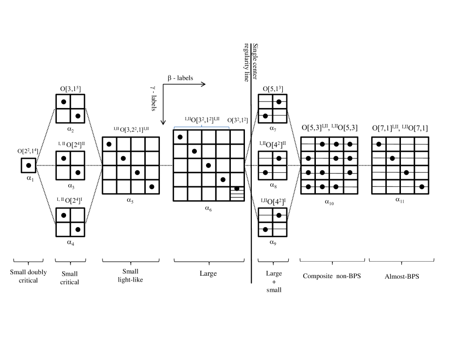
Figure 1. Schematic representations of the nilpotent orbits of $G_{0}={\rm SL}_{2}(\mathbb{R})^{4}$ on the coset space $\mathfrak{g}_{1}$ of ${\rm SO}(4,4)/{\rm SL}_{2}(\mathbb{R})^{4}$. Each square block represents an ${\rm SO}(4,4)^{\mathbb{C}}$-nilpotent orbit in its Lie algebra, while each column is in one-to-one correspondence with ${\rm SO}_{0}(4,4)$-nilpotent orbits in $\mathfrak{so}(4,4)$. For their description we use the notation of [30, 18, 13] (the trivial orbit $[1^{8}]$ is omitted). Thick vertical and horizontal lines separate orbits with distinct $\beta$- and $\gamma$-labels, respectively. The orbits $\alpha^{(2)},\alpha^{(3)},\alpha^{(4)}$ as well as the orbits $\alpha^{(7)},\alpha^{(8)},\alpha^{(9)}$ are related by STU triality, which is the outer-automorphism of the $D_{4}$ algebra $\mathfrak{g}^{c}$. The empty slots do not contain regular solutions [64]. The orbit structure with respect to the ${\rm SO}(2,2)^{2}$ subgroup of ${\rm SO}(4,4)$, which is relevant to the study of stationary solutions, is obtained by removing the thin horizontal lines in the $\alpha^{(7)},\dots,\alpha^{(11)}$-blocks, thus halving the corresponding number of cells and yielding a total of 101 orbits.

In Sections 4 and 5, as our first main result, we describe two methods for listing the nilpotent orbits of a real symmetric pair. Variations of these methods have been used in the literature, and to both we make useful additions. The general outline of these methods is the same: first one determines a finite set of nilpotent elements that contains representatives of all orbits; second, these elements are shown to be non-conjugate by using a variety of arguments. More precisely, in Section 4 we review the classification procedure of real nilpotent orbits used in [41]; this procedure is based on finding certain special $\mathfrak{sl}_{2}$-triples and uses tensor classifiers. However, it has not been shown in [41] that one can always find such triples. Here we rigorously prove that. For the implementation of this method we use the system Mathematica [71], mainly because of its equation solving abilities. In Section 5, we summarise the classification procedure based on Vinberg’s theory of carrier algebras [69], which was extended to the real case in [36]. In that paper some confusing assumptions have been posed on the Lie group that is used; we clarify this here. For the implementation of this method we use the computational algebra system GAP4 [45] and its package CoReLG [37].

We remark that Vân Lê [68] has developed a third strategy for listing the nilpotent orbits of a symmetric pair; however, her method requires to solve a difficult problem in algebraic geometry and therefore, to the best of our knowledge, has yet not led to a practical algorithm or implementation.

In Section 6, as our second main result, we introduce some mathematical invariants and methods for distinguishing real nilpotent orbits. We discuss the so-called $\alpha$-, $\beta$-, and $\gamma$-labels, tensor classifiers, and a (rather brute force) method based on solving polynomial equations using the technique of Gröbner bases.

We apply the two approaches described in Sections 4 and 5 to our main example of the STU model, and obtain the same classification. This classification is our third main result, and we report on our findings in Section 7. Here we note that both methods have their advantages and drawbacks: An advantage of the method based on ${\mathfrak{sl}}_{2}$-triples is that it produces so-called Cayley triples, which gives a straightforward algorithm to compute the $\beta$-label of the orbit. An advantage of the method based on carrier algebras is that it produces representatives with “nice” coefficients: in our main example, these coefficients are $\pm 1$, see the orbit representatives in Table I. Clearly, having two methods also allows for a convenient cross-validation of our classification results.

2. Background and physical motivation

One of the physical motivations behind the study of nilpotent orbits of real semisimple Lie groups is the problem of studying asymptotically-flat black hole solutions to extended (that is, $\mathcal{N}>1$) ungauged supergravities. These theories feature characteristic global symmetry groups of the field equations, and Bianchi identities. Such groups act on the scalar fields as isometry groups of the corresponding scalar manifold, and, at the same time, through generalised electric-magnetic transformations on the vector field strengths and their magnetic duals, see [42]. In [22] it was found that a subset of all solutions to the 4-dimensional theory, namely, the stationary (locally-)asymptotically-flat ones [58, 61, 62, 2], actually feature a larger symmetry group $G$ which is not manifest in four space-time dimensions ($D=4$), but rather in an effective Euclidean 3-dimensional description which is formally obtained by compactifying the 4-dimensional model along the time direction and dualising the vector fields into scalars. Stationary 4-dimensional asymptotically-flat black hole solutions can be conveniently arranged in orbits with respect to this larger symmetry group $G$, whose action has proven to be a valuable tool for their classification (see [33, 48, 43, 10, 19, 26, 18, 52, 24, 41, 20, 15, 25]). It also yields a “solution-generating technique” (see [33]) for constructing new solutions from known ones (see [32, 4, 6, 29, 28]).

2.1. Asymptotically flat black holes and nilpotent orbits

In the effective $D=3$ description, stationary asymptotically-flat 4-dimensional black holes are solutions to an Euclidean non-linear sigma-model coupled to gravity, the target space being a pseudo-Riemannian manifold $\mathcal{M}$ of which $G$ is the isometry group. Such solutions are described by a set of scalar fields $\phi^{I}(x^{i})$ parametrising $\mathcal{M}$, which are functions of the three spatial coordinates $x^{1},x^{2},x^{3}$; in the axisymmetric solutions the dependence is restricted to the polar coordinates $(r,\theta)$ only. The asymptotic data defining the solution comprise the value $\phi_{0}\equiv(\phi^{I}_{0})$ of the scalar fields at radial infinity and the Noether charge matrix $Q$, which is associated with the global symmetry group of the sigma-model and which has value in the Lie algebra $\mathfrak{g}$ of $G$. If $\mathcal{M}$ is homogeneous, then we can always fix $G$ to map the point at infinity $\phi_{0}$ into the origin $O$, where the invariance under the isotropy group $G_{0}$ of $\mathcal{M}$ is manifest. We restrict ourselves only to models in which $\mathcal{M}$ is homogeneous symmetric of the form $\mathcal{M}=G/G_{0}$. The solutions are therefore classified according to the action of $G_{0}$ (residual symmetry at the origin) on the Noether charge matrix $Q$, seen as an element of the tangent space to the manifold in $O$. The rotation of the solution is encoded in another $\mathfrak{g}$-valued matrix $Q_{\psi}$, first introduced in [5, 4], which contains the angular momentum of the solution as a characteristic component and vanishes in the static limit. Once we fix $\phi_{0}\equiv O$, both $Q$ and $Q_{\psi}$ become elements of the coset space ${\mathfrak{g}}_{1}$ (which is isomorphic to the tangent space at the origin) and thus transform under $G_{0}$. The action of $G$ on the whole solution amounts to the action of $G_{0}$ on $Q$ and $Q_{\psi}$.

Non-extremal (or extremal over-rotating) solutions are characterized by matrices $Q$ and $Q_{\psi}$ belonging to the same regular $G_{0}$-orbit which contains the Kerr (or the extremal-Kerr) solution. In the so-called STU model, which is an $\mathcal{N}=2$ supergravity coupled to three vector multiplets, the most general representative of the Kerr-orbit was derived in [29, 28] and features all the duality-invariant properties of the most general solution to the maximal (ungauged) supergravity of which the STU model is a consistent truncation. (The name of this model comes from the conventional notation $S$, $T$, and $U$ for the three complex scalar fields in these multiplets). On the other hand, extremal static and under-rotating solutions [63, 56, 7] feature nilpotent $Q$ and $Q_{\psi}$ which belong to different orbits of $G_{0}$. The classification of these solutions is therefore intimately related to the classification of the nilpotent orbits in a given representation $\rho$ of a real non-compact semisimple Lie group – which is the general mathematical problem we focus on in this paper: here the representation $\rho$ is defined by the adjoint action of $G_{0}$ on the coset space $\mathfrak{g}_{1}$ which $Q$ and $Q_{\psi}$ belong to, once we fix $\phi_{0}\equiv O$.

Stationary extremal solutions have been studied in [18, 20, 15] in terms of the nilpotent orbits of the complexification $G^{c}_{0}$ of $G_{0}$; the latter are known from the mathematical literature. As far as single-center solutions are concerned, as mentioned in the introduction, these orbits, as opposed to the real ones, do not provide an intrinsic characterisation of regular single-center solutions, since in general they contain singular solutions as well as regular ones. A classification of real nilpotent orbits has been performed in specific $\mathcal{N}=2$ ungauged models [40, 41, 25], in connection to the study of their extremal 4-dimensional solutions. There it is shown that, at least for single-center black holes, there is a one-to-one correspondence between the regularity of the solutions (as well as their supersymmetry) and certain real nilpotent orbits. This allows us to check the regularity of the solution by simply inspecting the corresponding $G_{0}$-orbit. The classification procedure adopted in [40, 41, 25] combines the method of standard triples [30] with new techniques based on the Weyl group: After a general group theoretical analysis of the model, this approach allows for a systematic construction of the various nilpotent orbits by solving suitable matrix equations in nilpotent generators. Solutions to these equations belong to the same $G_{0}^{c}$-orbit, but in general to different $G_{0}$-orbits. The final step is to group the solutions under the action of $G_{0}$. Solutions which are not in the same $G_{0}$-orbit are distinguished by certain $G_{0}$-invariants, amongst others, tensor classifiers, that is, signatures of suitable $G_{0}$-covariant symmetric tensors. This ensures that the classification is complete.

The main difficulty in determining the nilpotent $G_{0}$-orbits in $\mathfrak{g}_{1}$ is that such orbits are not completely classified by the intersection of the $G_{0}^{c}$-orbits in $\mathfrak{g}_{1}^{c}$ and the $G$-orbits in its Lie algebra $\mathfrak{g}$, both of which are known: The former are completely classified by the so-called $\gamma$-labels; the latter by the so-called $\beta$-labels obtained by the Kostant-Sekiguchi Theorem. These two labels do not provide a complete classification of the real nilpotent orbits, as it was shown in an explicit example in [25]. Distinct $G_{0}$-orbits having the same $\gamma$- and the same $\beta$-labels can be characterised using $G_{0}$-invariant quantities, like tensor classifiers, and will be distinguished by a further label $\delta$. We refer to Section 6.4 for a precise definition of all the aforementioned labels.

2.2. Our main example

Of particular interest are the multi-center solutions like the almost-BPS ones [46, 9, 34, 44] and the composite non-BPS ones [20]. These are extremal solutions (with zero Hawking temperature), characterised by nilpotent matrices $Q$ and $Q_{\psi}$. Since the geometries of the horizons surrounding each center are affected by subleading corrections (due to the interaction with the other centers), the regularity of the whole solution implies that each center, if isolated from the others, is regular [20]. Real nilpotent orbits (namely, the $G_{0}$-orbits in $\mathfrak{g}_{1}$), as opposed to the complex ones, provide an intrinsic characterisation of regular single center solutions, and thus are a valuable tool for constructing regular multi-center solutions: A necessary condition for a multi-center solution to be regular is that the Noether charge of each of its centers belongs to real orbits which correspond to regular single-center solutions, their sum coinciding with the total Noether charge. A detailed discussion of this matter (in relation to multi-center solutions) is given in [64]; the aim of the present paper is to illustrate the importance of considering real nilpotent orbits: we show that a complex orbit contains solutions which, although exhibiting an acceptable behaviour of the metric close to the center and at infinity, feature singularities at finite distances from the center.

For this purpose we consider solutions to the simple $D=4$ STU model, see for instance [10, 20]. The corresponding effective $D=3$ description of stationary solutions has $G={\rm SO}(4,4)$ as global symmetry group and the scalar fields span the manifold $\mathcal{M}_{\rm scal}=G/G_{0}^{\prime}$ with isotropy group

$$G_{0}^{\prime}=({\rm SO}(2,2))^{2}={\rm SO}(2,2)\times{\rm SO}(2,2),$$

where ${\rm SO}(2,2)={\rm SL}_{2}(\mathbb{R})\times_{\mathbb{Z}_{2}}{\rm SL}_{2}(\mathbb{R})$ is a central product of two ${\rm SL}_{2}(\mathbb{R})$. The Lie group $G_{0}^{\prime}$ is locally isomorphic to

$$G_{0}=({\rm SL}_{2}(\mathbb{R}))^{4}$$

as it has the same Lie algebra as $G_{0}$. The extremal solutions, once we fix $\phi_{0}\equiv O$, are characterised by a Noether charge matrix $Q$ in some nilpotent orbit of $G_{0}^{\prime}$ over the coset space $\mathfrak{g}_{1}$. This is the example we explicitly work out in the present paper, with the difference that we actually consider $G_{0}$-orbits rather than $G_{0}^{\prime}$-orbits. In Table I, we list $G_{0}$-orbit representatives and associated $\alpha$-, $\beta$-, and $\gamma$-labels. The classification of the orbits with respect to $G_{0}$ only differs from that corresponding to $G_{0}^{\prime}$ by a simple identification. This identification is described by the following rule, for whose explanation we refer to [64]. In Table I, every pair of $G_{0}$-orbits which have the same $\alpha$-label in $\{\alpha^{(7)},\ldots,\alpha^{(11)}\}$, coinciding $\gamma$- and coinciding $\beta$-labels, and which are otherwise only distinguished by $\delta^{(1)}$ and $\delta^{(2)}$, define the same $G_{0}^{\prime}$-orbit: for example, the two $G_{0}$-orbits with labels $\alpha^{(10)}\beta^{(10;1)}\gamma^{(10;2)}\delta^{(1)}$ and $\alpha^{(10)}\beta^{(10;1)}\gamma^{(10;2)}\delta^{(2)}$ define the same $G_{0}^{\prime}$-orbit. We obtain $145$ orbits under $G_{0}$, and these reduce to $101$ orbits under $G_{0}^{\prime}$.

For regular or small (that is, with vanishing horizon area) single-center extremal solutions, $Q$ (in the fundamental representation of $G$) must have a degree of nilpotency not exceeding 3. This restricts the $\alpha$-label to be in the set $\{\alpha^{(1)},\dots,\alpha^{(6)}\}$. More specifically, they are characterised by coinciding $\gamma$- and $\beta$- labels [52, 25]. Orbits with $\alpha$-label in the set $\{\alpha^{(7)},\dots,\alpha^{(11)}\}$ can only describe regular multi-center solutions [20]. Regular single-center solutions correspond to orbits with $\alpha$-label $\alpha^{(6)}$. As far as the static solutions are concerned, we have three types:

i)	$\alpha^{(6)}$, $\gamma^{(6;1)}$, $\beta^{(6;1)}$	(BPS solutions)
ii)	$\alpha^{(6)}$, $\gamma^{(6;2,3,4)}$, $\beta^{(6;2,3,4)}$	(non-BPS solutions with vanishing central charge at the horizon)
iii)	$\alpha^{(6)}$, $\gamma^{(6;5)}$, $\beta^{(6;5)}$, $\delta^{(1)}$	(non-BPS solutions with non-vanishing central charge at the horizon).

These orbits correspond to the classification of 4-dimensional regular static solutions obtained in [8]. The complex nilpotent orbits are only characterised by the $\alpha$- and $\gamma$-labels, and thus comprise real orbits with different $\beta$-labels – some of which describe solutions featuring singularities at finite radial distance from the centers. To illustrate this, it is useful to describe the single-center generic representative of the orbits with $\alpha$-label ranging from $\alpha^{(1)}$ to $\alpha^{(6)}$ in terms of the generating solution [10, 26, 25] (that is, the representative of the real orbits which depends on the least number of parameters). The space-time metric is expressed in terms of four harmonic functions

(2.1) $${\bf H}_{0}=1-k_{0}\,\tau=1-\sqrt{2}\,\epsilon_{0}\,q_{0}\,\tau\quad\text{and}\quad{\bf H}_{\ell}=1-k_{\ell}\,\tau=1-\sqrt{2}\,\epsilon_{\ell}\,p^{\ell}\,\tau\quad(\ell=1,2,3),$$

where $\epsilon_{\ell}=\pm 1$ and $\ell=0,1,2,3$ and $\tau\equiv-1/r$ (with $r$ being the radial distance from the center), and $q_{0},p^{1},p^{2},p^{3}$ are the electric ($q_{0}$) and magnetic ($p^{\ell}$) charges of the solution. The metric of the static solution reads

$${\rm d}s^{2} =-e^{2U}\,{\rm d}t^{2}+e^{-2U}\,({\rm d}r^{2}+r^{2}{\rm d}\theta^{2}+r^{2}\sin^{2}(\theta){\rm d}\varphi^{2})\quad,$$

(2.2) $$e^{-2U} =\sqrt{{\bf H}_{0}{\bf H}_{1}{\bf H}_{2}{\bf H}_{3}}\qquad\text{and}\qquad e^{\varphi_{i}}=\sqrt{({\bf H}_{0}{\bf H}_{i})/({\bf H}_{j}{\bf H}_{k})}\text{ with }\{i,j,k\}=\{1,2,3\},\quad$$

where $e^{\varphi_{i}}$ are the imaginary parts of the three complex scalars, the real parts being zero on the solution. Asymptotic flatness requires $\lim_{r\rightarrow\infty}U(r)=0$. As shown in [25], the $\gamma$-label of the orbit only depends on $\epsilon_{\ell}k_{\ell}^{2}$ while the $\beta$-label depends on $\epsilon_{\ell}k_{\ell}$, $\ell=0,1,2,3$; they coincide only for $k_{\ell}>0$, which is the necessary and sufficient condition for regularity. Indeed, if one of the $k_{\ell}$ were negative, then some of the harmonic functions would have a zero root, and the metric a singularity at finite $r$ (or, equivalently, $\tau$). One can show that this value of $r$ corresponds to a curvature singularity. The area of the horizon is given by

(2.3) $$A_{\rm H}=4\pi\lim_{\tau\rightarrow-\infty}e^{-2U}/\tau^{2}=4\pi\sqrt{k_{0}k_{1}k_{2}k_{3}},$$

while the ADM mass reads

(2.4) $$M_{{\rm ADM}}=\lim_{\tau\rightarrow 0^{-}}\dot{U}=(k_{0}+k_{1}+k_{2}+k_{3})/4\,.$$

We see that if only two of the $k_{\ell}$ are negative, then the solution can be singular, but with acceptable near-horizon limit (according to (2.3)) and positive ADM mass (2.4). This is illustrated in Figure 2, where we consider (single-center) representatives of real orbits within the same complex one. It is shown that within the complex orbit of the BPS solutions (defined by $\gamma^{(6;1)}$) and of the non-BPS solutions of type iii) (defined by $\gamma^{(6;5)}$), one can find solutions (Figures 2a) and 2c)) which cannot be distinguished from the regular ones by the asymptotic behaviour of their metric at $r\rightarrow 0$ and $r\rightarrow\infty$, but which feature singularities at finite $r$. Such solutions are distinguished from the regular ones by their real nilpotent orbits. Therefore the framework of real nilpotent orbits is the appropriate one to characterise, in an intrinsic algebraic way, the regularity of single and multi-center solutions to ungauged supergravity. An equivalent approach is to implement regularity directly on the solution, as it is done in [21] where a detailed analysis is made of the composite non-BPS solutions and a characterization of the regularity of each center (in the $G_{4}$-orbit $I_{4}<0$) is given as the requirement that a given charge-dependent, Jordan-algebra valued matrix be positive definite.

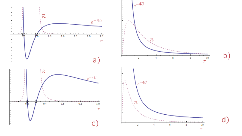
Figure 2. Behaviour of the warp function $e^{-4U}$ and of the Ricci scalar $\mathcal{R}$ against $r$ for representatives of selected real orbits. Fig. a): representative of the $(\gamma^{(6;1)},\,\beta^{(6;2)})$ orbit corresponding to a singular BPS solution (singularities being marked by a circle); Fig. b): representative of the $(\gamma^{(6;1)},\,\beta^{(6;1)})$ orbit corresponding to a regular BPS solution; Fig. c): representative of the $(\gamma^{(6;5)},\,\beta^{(6;5)},\,\delta^{(2)})$ orbit corresponding to a singular non-BPS solution (singularities being marked by a circle); Fig. d): representative of the $(\gamma^{(6;5)},\,\beta^{(6;5)},\,\delta^{(1)})$ orbit corresponding to a regular non-BPS solution of type iii). Solutions a) and b) belong to the same complex orbit defined by $\gamma^{(6;1)}$, and similarly c) and d) belong to the same complex orbit defined by $\gamma^{(6;5)}$. Clearly the values of $\mathcal{R}$ and of $e^{-4U}$ refer to different scales. They are plotted in the same graphs to illustrate the corresponding behaviours at the same values of $r$.

Real orbits with $\alpha$-label ranging from $\alpha^{(1)}$ to $\alpha^{(5)}$ and $\gamma=\beta$ describe small black holes, namely extremal single center solutions with vanishing horizon area. Such solutions are classically singular, though the singularity coincides with the center ($r=0$). Solutions in orbits with $\gamma\neq\beta$, on the other hand, just as for the $\alpha^{(6)}$-orbits, feature singularities at finite nonzero $r$. Small black hole solutions were classified in [14]: $\alpha^{(1)},\,\gamma^{(1;1)}=\beta^{(1;1)}$ corresponds to the doubly critical solutions; $\alpha^{(2)},\,\gamma^{(2;\ell)}=\beta^{(2;\ell)}$, $\alpha^{(3)},\,\gamma^{(3;\ell)}=\beta^{(3;\ell)}$ and $\alpha^{(4)},\,\gamma^{(4;\ell)}=\beta^{(4;\ell)}$ to the critical solutions; $\alpha^{(5)},\,\gamma^{(5;\ell)}=\beta^{(5;\ell)}$ to the light-like small solutions. The first representatives (corresponding to $\ell=1$) of each set of orbits describe solutions preserving an amount of supersymmetry (BPS solutions)

In [64] a composition rule of the 16 real orbits describing regular (small and large) single-center solutions into the higher order $\alpha^{(7)}-\alpha^{(11)}$-orbits is defined: generic representatives $e$ and $e^{\prime}$ of two regular-single-center orbits $\mathcal{O}$ and $\mathcal{O}^{\prime}$ are combined into a nilpotent representative of a higher order orbit $\mathcal{O}^{\prime\prime}$, under the general assumption that the corresponding neutral elements $h$ and $h^{\prime}$ commute. A composition law is defined $\mathcal{O},\,\mathcal{O}^{\prime}\rightarrow\mathcal{O}^{\prime\prime}$ and it is observed that some of the $\alpha^{(7)}-\alpha^{(11)}$-orbits are never obtained in this way. Such orbits are characterized as intrinsically singular in that they contain no regular solution. They are represented by empty slots in Figure 1.

3. The mathematical framework

In this section we define a symmetric pair $({\mathfrak{g}},{\mathfrak{g}}_{0})$ and a class of Lie groups $G_{0}$ acting on ${\mathfrak{g}}_{1}$; we also introduce the main example motivated in Section 2.2. The notation introduced in this section is retained throughout the paper.

3.1. The symmetric pair $({\mathfrak{g}},{\mathfrak{g}}_{0})$

Let ${\mathfrak{g}}$ be a semisimple Lie algebra over the real numbers. We assume throughout that ${\mathfrak{g}}$ is split, that is, it has a Cartan subalgebra ${\mathfrak{h}}$ that is split over the reals; every complex semisimple Lie algebra contains such a split real form (see [53, Corollary 6.10]). Let $\varphi\colon{\mathfrak{g}}\to{\mathfrak{g}}$ be an automorphism of order 2 with eigenspace decomposition ${\mathfrak{g}}={\mathfrak{g}}_{0}\oplus{\mathfrak{g}}_{1}$, where $\varphi$ has eigenvalue $(-1)^{i}$ on ${\mathfrak{g}}_{i}$. The pair $({\mathfrak{g}},{\mathfrak{g}}_{0})$ is a real symmetric pair; note that the decomposition ${\mathfrak{g}}={\mathfrak{g}}_{0}\oplus{\mathfrak{g}}_{1}$ is a $\mathbb{Z}/2\mathbb{Z}$-grading of ${\mathfrak{g}}$, that is, $[{\mathfrak{g}}_{i},{\mathfrak{g}}_{j}]\subseteq{\mathfrak{g}}_{i+j\bmod 2}$ for $i,j\in\{0,1\}$.

Let $\theta\colon{\mathfrak{g}}\to{\mathfrak{g}}$ be a Cartan involution of ${\mathfrak{g}}$ commuting with $\varphi$; such a Cartan involution exists and is unique up to conjugacy by an element in $\exp(\mathop{\rm ad}_{\mathfrak{g}}({\mathfrak{g}}_{0}))$, see for example [65, Theorem 1.1]. Let ${\mathfrak{g}}={\mathfrak{k}}\oplus{\mathfrak{p}}$ be the Cartan decomposition associated with $\theta$; this decomposition is also a $\mathbb{Z}/2\mathbb{Z}$-grading of ${\mathfrak{g}}$. Since any Cartan subalgebra of ${\mathfrak{g}}$ is conjugate to a $\theta$-stable Cartan subalgebra (​[53, Proposition 6.59]), we may assume that the split Cartan subalgebra ${\mathfrak{h}}$ of ${\mathfrak{g}}$ is $\theta$-stable; this implies that ${\mathfrak{h}}\subseteq{\mathfrak{p}}$, because ${\mathfrak{h}}$ is split. Since $\theta$ and $\varphi$ commute, the two gradings are compatible, that is ${\mathfrak{g}}_{0}=({\mathfrak{g}}_{0}\cap{\mathfrak{k}})\oplus({\mathfrak{g}}_{0}\cap{\mathfrak{p}})$, and similarly for ${\mathfrak{g}}_{1}$.

We exemplify the results of our paper by a detailed discussion of the following example, which is motivated by the discussion in Section 2.2.

Example 1.

Let ${\mathfrak{g}}$ be the real Lie algebra defined by

$${\mathfrak{g}}=\{X\in{\mathfrak{gl}}_{8}(\mathbb{R})\mid X^{\intercal}M=-MX\}\quad\text{where}\quad M=\left(\begin{smallmatrix}0&I_{4}\\ I_{4}&0\end{smallmatrix}\right),$$

with $I_{4}$ the $4\times 4$ identity matrix; this is the split Lie algebra of type $D_{4}$, see [51, Theorem IV.9]. Here we consider the involution $\varphi\colon{\mathfrak{g}}\to{\mathfrak{g}}$, $X\mapsto DXD$, where $D=\mathrm{diag}(1,1,-1,-1,1,1,-1,-1)$. A Cartan involution of ${\mathfrak{g}}$ commuting with $\varphi$ is negative-transpose, that is, $\theta(X)=-X^{\intercal}$. These involutions can also conveniently be described by their action on a suitable generating set of ${\mathfrak{g}}$. In the following let $e_{ij}$ be the $8\times 8$ matrix with a $1$ on position $(i,j)$ and zeros elsewhere; for $i\in\{1,\ldots,4\}$ define $d_{i}=e_{ii}-e_{4+i,4+i}$, so that $\{d_{1},\ldots,d_{4}\}$ spans a Cartan subalgebra of ${\mathfrak{g}}$. Now define $h_{1}=d_{1}-d_{2}$, $h_{2}=d_{2}-d_{3}$, $h_{3}=d_{3}+d_{4}$, $h_{4}=d_{3}-d_{4}$, $e_{1}=e_{12}-e_{65}$, $e_{2}=e_{23}-e_{76}$, $e_{3}=e_{38}-e_{47}$, $e_{4}=e_{34}-e_{87}$, and, lastly, $f_{i}=e_{i}^{\intercal}$ for $1\leq i\leq 4$. A straightforward computation shows that these elements satisfy the following relations

$${}[h_{i},h_{j}] =0,\qquad [h_{i},e_{j}] =C_{j,i}e_{j},$$

$$[e_{i},f_{j}] =\delta_{ij}h_{i}, [h_{i},f_{j}] =-C_{j,i}f_{j},$$

where $\delta_{ij}$ is the Kronecker delta and $C_{i,j}$ is the entry $(i,j)$ of the Cartan matrix $C$ of the root system of type $D_{4}$ with Dynkin diagram

By [51, §IV.3], the set $\{h_{i},e_{i},f_{i}\mid i\in\{1,\ldots,4\}\}$ is a canonical generating set of ${\mathfrak{g}}$; in particular, an automorphism of ${\mathfrak{g}}$ is uniquely determined by its values on these elements. It follows readily from the definition that $\theta(e_{i})=-f_{i}$, $\theta(f_{i})=-e_{i}$, and $\theta(h_{i})=-h_{i}$ for all $i$; moreover, $\varphi(e_{i})=e_{i}$, $\varphi(f_{i})=f_{i}$ for $i\neq 2$, $\varphi(e_{2})=-e_{2}$, $\varphi(f_{2})=-f_{2}$, and $\varphi(h_{j})=h_{j}$ for all $j$. It follows that $\dim{\mathfrak{k}}=\dim{\mathfrak{g}}_{0}=12$ and $\dim{\mathfrak{p}}=\dim{\mathfrak{g}}_{1}=16$. It is straightforward to work out bases for these subspaces; for example, ${\mathfrak{g}}_{0}$ is spanned by $\{h_{i},e_{i},f_{i}\mid i=1,3,4\}$ along with $e_{0}=e_{16}-e_{25}$, $f_{0}=e_{0}^{\intercal}$, and $h_{0}=d_{1}+d_{2}$. It follows that ${\mathfrak{g}}_{0}$ is isomorphic to the direct sum of four copies of ${\mathfrak{sl}}_{2}(\mathbb{R})$. $\bullet$

Here and in the sequel we denote by ${\mathfrak{g}}^{c}=\mathbb{C}\otimes_{\mathbb{R}}{\mathfrak{g}}$ the complexification of ${\mathfrak{g}}$ and by $\mathop{\rm ad}\colon{\mathfrak{g}}^{c}\to{\rm End}({\mathfrak{g}}^{c})$ its adjoint map, that is, $\mathop{\rm ad}(x)\colon{\mathfrak{g}}^{c}\to{\mathfrak{g}}^{c}$, $y\mapsto[x,y]$. If we use the adjoint map of a different Lie algebra, then we use a subscript, for example $\mathop{\rm ad}_{\mathfrak{g}}\colon{\mathfrak{g}}\to{\rm End}({\mathfrak{g}})$. Note that $\varphi$ lifts to an involution of ${\mathfrak{g}}^{c}$, with eigenspace decomposition ${\mathfrak{g}}^{c}={\mathfrak{g}}_{0}^{c}\oplus{\mathfrak{g}}_{1}^{c}$.

3.2. The Lie groups $G_{0}$

We continue with the notation of the previous section, and denote by $G^{c}$ the adjoint group of ${\mathfrak{g}}^{c}$. This group can be characterised in various ways: It is the connected algebraic subgroup of ${\rm GL}({\mathfrak{g}}^{c})$ with Lie algebra $\mathop{\rm ad}({\mathfrak{g}}^{c})$ (see [30, §1.2]); it is also the connected component of the automorphism group of ${\mathfrak{g}}^{c}$, and generated by inner automorphisms $\exp(\mathop{\rm ad}(x))$ with $x\in{\mathfrak{g}}$ (see [60, (I.7)]). In any way, $G^{c}$ is a subgroup of the automorphism group of ${\mathfrak{g}}^{c}$. We denote by $G_{0}^{c}$ the connected algebraic subgroup of $G^{c}$ with Lie algebra $\mathop{\rm ad}({\mathfrak{g}}_{0}^{c})$; alternatively, this is the subgroup of $G^{c}$ generated by all $\exp(\mathop{\rm ad}(x))$ with $x\in{\mathfrak{g}}_{0}^{c}$.

Let $\mathcal{N}_{1}^{c}$ be the set of nilpotent elements in ${\mathfrak{g}}_{1}^{c}$; the determination of $G_{0}^{c}$-orbit representatives in $\mathcal{N}_{1}^{c}$ has been discussed in the literature and we recall some of the main results in Sections 4.1 and 5.1. Our main focus here is the determination of representatives in $\mathcal{N}_{1}$, the set of nilpotent elements in ${\mathfrak{g}}_{1}$, under the action of a suitable group $G_{0}$. There are different interesting choices for $G_{0}$. For example, one could define $G_{0}$ as the adjoint group of ${\mathfrak{g}}_{0}$, which is the analytic subgroup of ${\rm GL}({\mathfrak{g}}_{0})$ with Lie algebra $\mathop{\rm ad}_{\mathfrak{g}}({\mathfrak{g}}_{0})$ (see [49, §II.5]). Alternatively, one could define $G_{0}$ as the set of real points $G_{0}^{c}(\mathbb{R})$, that is, the subgroup of elements of $G_{0}^{c}\subseteq{\rm GL}({\mathfrak{g}}^{c})$ whose matrix (with respect to some fixed basis of ${\mathfrak{g}}^{c}$ consisting of elements of ${\mathfrak{g}}$) has real entries only. We aim to provide a framework which allows us to deal with several different choices of $G_{0}$.

More precisely, here we define a group $G_{0}$ acting on ${\mathfrak{g}}_{1}$ as follows; we exemplify our construction in Example 4 below. We start with an isomorphism of algebraic groups $R^{c}\colon\widetilde{G}_{0}^{c}\to G_{0}^{c}$, where $\widetilde{G}_{0}^{c}$ is a connected algebraic subgroup of ${\rm GL}_{k}(\mathbb{C})$ for some $k$; we also assume that both $\widetilde{G}_{0}^{c}$ and $R^{c}$ are defined over $\mathbb{R}$. We define $\widetilde{G}_{0}=\widetilde{G}^{c}_{0}(\mathbb{R})$ as the group consisting of all $g\in\widetilde{G}^{c}_{0}$ with coefficients in $\mathbb{R}$, and then define

$$G_{0}=R^{c}(\widetilde{G}^{c}_{0}(\mathbb{R})).$$

It follows from [11, §7.3] that the isomorphism $R^{c}$ induces a (not necessarily surjective) embedding of $\widetilde{G}_{0}^{c}(\mathbb{R})$ into $G_{0}^{c}(\mathbb{R})$ which maps the identity component of $\widetilde{G}_{0}^{c}(\mathbb{R})$ onto that of $G_{0}^{c}(\mathbb{R})$; moreover $G_{0}$ is closed and has finite index in $G_{0}^{c}(\mathbb{R})$. We note that the group $G_{0}^{c}(\mathbb{R})$ has finitely many connected components, cf. [12, p. 276 (c)(i)]. In conclusion, we have

$$(G_{0}^{c}(\mathbb{R}))^{\circ}\leq G_{0}\leq G_{0}^{c}(\mathbb{R})\leq{\rm Aut}({\mathfrak{g}})\leq{\rm Aut}({\mathfrak{g}}^{c}).$$

Here $(G_{0}^{c}(\mathbb{R}))^{\circ}$ denotes the identity component of $G_{0}^{c}(\mathbb{R})$ (in the real Euclidean topology), which is the same as the identity component of $G_{0}$. The groups $(G_{0}^{c}(\mathbb{R}))^{\circ}$, $G_{0}$, and $G_{0}^{c}(\mathbb{R})$ all have the same Lie algebra, which is $\mathop{\rm ad}_{\mathfrak{g}}({\mathfrak{g}}_{0})\cong{\mathfrak{g}}_{0}$.

Recall that a Lie algebra is reductive if it is the direct sum of its semisimple derived subalgebra and its center. It is well-known that ${\mathfrak{g}}_{0}$ is a reductive Lie algebra; more precisely, it is “reductive in ${\mathfrak{g}}$” (see for example [36]). There exist different definitions for a Lie group to be reductive; here we use the quite technical definition given in [53, Section VII.2]), mainly because this allow us to use the results in [53, Chapter VII] for reductive groups.

Definition 2.

A real Lie group $\mathcal{G}$ is reductive if there is a quadruple $(\mathcal{G},\mathcal{K},\eta,\mathcal{B})$, where $\mathcal{K}\leq\mathcal{G}$ is a compact subgroup, $\eta$ is an involution of the Lie algebra $\mathbf{g}$ of $\mathcal{G}$, and $\mathcal{B}$ is a nondegenerate $\mathrm{Ad}(\mathcal{G})$- and $\eta$-invariant bilinear form on $\mathbf{g}$, such that the following hold:

• $\mathbf{g}$ is reductive,

• the $\pm 1$-eigenspace decomposition of $\eta$ is $\mathbf{g}=\mathbf{k}\oplus\mathbf{p}$, where $\mathbf{k}$ is the Lie algebra of $\mathcal{K}$,

• $\mathbf{k}$ and $\mathbf{p}$ are orthogonal under $\mathcal{B}$, and $\mathcal{B}$ is negative definite on $\mathbf{k}$ and positive definite on $\mathbf{p}$,

• the multiplication map $\mathcal{K}\times\exp(\mathbf{p})\to\mathcal{G}$ is a surjective diffeomorphism,

• for each $g\in\mathcal{G}$, the automorphism $\mathrm{Ad}(g)$ of $\mathbf{g}^{c}$ is inner, that is, it lies in $\mathrm{Int}(\mathbf{g}^{c})$.

If $\mathcal{G}$ is a closed linear Lie group, then $\mathrm{Ad}(g)(x)=gxg^{-1}$ for $x\in\mathbf{g}$ and $g\in\mathcal{G}$, see [53, p. 79]. Recall that $\mathrm{Int}(\mathbf{g}^{c})$ is the analytic subgroup of ${\rm Aut}(\mathbf{g}^{c})$ with Lie algebra $\mathop{\rm ad}(\mathbf{g}^{c})$, generated by all $\exp(\mathop{\rm ad}(x))$ with $x\in\mathbf{g}^{c}$, see [60, p. 1]. It contains the connected algebraic subgroup of ${\rm Aut}(\mathbf{g}^{c})$ with Lie algebra $\mathop{\rm ad}(\mathbf{g}^{c})$.

Proposition 3.

The group $G_{0}$ is a reductive Lie group.

• We first show that $G=G^{c}(\mathbb{R})$ is reductive. Firstly, $G$ has Lie algebra $\mathop{\rm ad}_{\mathfrak{g}}({\mathfrak{g}})$, which is semisimple, hence reductive. It follows from [60, §5.(5)] that $\mathop{\rm ad}_{\mathfrak{g}}({\mathfrak{g}})$ has the inner product $(\mathop{\rm ad}_{\mathfrak{g}}(x),\mathop{\rm ad}_{\mathfrak{g}}(y))=-\kappa(x,\theta(y))$, where $\kappa$ is the Killing form of ${\mathfrak{g}}^{c}$. Let $O(\mathop{\rm ad}_{\mathfrak{g}}({\mathfrak{g}}))$ be the group of all bijective endomorphisms of $\mathop{\rm ad}_{\mathfrak{g}}({\mathfrak{g}})$ that leave this inner product invariant, and define $K=\{g\in G\mid\mathrm{Ad}(g)\in O(\mathop{\rm ad}_{\mathfrak{g}}({\mathfrak{g}}))\}$. Define a bilinear form $B$ on $\mathop{\rm ad}_{\mathfrak{g}}({\mathfrak{g}})$ by $B(\mathop{\rm ad}\nolimits_{\mathfrak{g}}(x),\mathop{\rm ad}\nolimits_{\mathfrak{g}}(y))=\kappa(x,y)$. We extend the Cartan involution $\theta$ of ${\mathfrak{g}}$ to an automorphism of $\mathop{\rm ad}_{\mathfrak{g}}({\mathfrak{g}})$ by setting $\theta(\mathop{\rm ad}_{\mathfrak{g}}(x))=\mathop{\rm ad}_{\mathfrak{g}}(\theta(x))$. We claim that $(G,K,\theta,B)$ satisfies Definition 2. Similarly to $\mathop{\rm ad}_{\mathfrak{g}}({\mathfrak{g}})$, the Lie algebra ${\mathfrak{g}}$ has an inner product defined by $(x,y)=-\kappa(x,\theta(y))$. Let $O({\mathfrak{g}})$ be the group of bijective endomorphisms of ${\mathfrak{g}}$ leaving this inner product invariant. Using [53, Lemma 1.118], one sees that $K=G\cap O({\mathfrak{g}})$, and as $K$ is closed, it follows that it is compact. By [53, Proposition 1.119], the Killing form is invariant under ${\rm Aut}({\mathfrak{g}}^{c})$, which implies that $B$ is $\mathrm{Ad}(G)$- and $\theta$-invariant; since $\kappa$ is nondegenerate on ${\mathfrak{g}}$, so is $B$. Clearly, $\theta$ is a Cartan involution with Cartan decomposition $\mathop{\rm ad}_{\mathfrak{g}}({\mathfrak{g}})=\mathop{\rm ad}_{\mathfrak{g}}({\mathfrak{k}})\oplus\mathop{\rm ad}_{\mathfrak{g}}({\mathfrak{p}})$. Since the latter is a $\mathbb{Z}/2\mathbb{Z}$-grading, $\mathop{\rm ad}_{\mathfrak{g}}({\mathfrak{k}})$ and $\mathop{\rm ad}_{\mathfrak{g}}({\mathfrak{p}})$ are orthogonal under $B$. Moreover, $B$ is positive definite on $\mathop{\rm ad}_{\mathfrak{g}}({\mathfrak{p}})$ and negative definite on $\mathop{\rm ad}_{\mathfrak{g}}({\mathfrak{k}})$ by [60, §5 (5) & (6)]. Note that the Lie algebra of $G$ is semisimple, so that $G$ is semisimple (see [59, p. 56]). This allows us to apply [59, §5.3, Theorem 2 & Corollary 2], which proves that (iv) of Definition 2 holds, and that the Lie algebra of $K$ is $\mathop{\rm ad}_{\mathfrak{g}}({\mathfrak{k}})$. To establish (v) of Definition 2, consider $g\in G$. Since $G$ is a closed linear group, $\mathrm{Ad}(g)(\mathop{\rm ad}_{\mathfrak{g}}(x))=g(\mathop{\rm ad}_{\mathfrak{g}}(x))g^{-1}$ for all $x\in{\mathfrak{g}}$ by [53, p. 79]; now [53, Lemma 1.118] shows that $g(\mathop{\rm ad}_{\mathfrak{g}}(x))g^{-1}=\mathop{\rm ad}_{\mathfrak{g}}g(x)$, which proves that $\mathrm{Ad}(g)$ is induced by the automorphism $g$; as $G\leq G^{c}\leq\mathrm{Int}({\mathfrak{g}}^{c})$, we obtain (v).

  Now we consider $G_{0}$. By abuse of notation we also use the symbols $\theta$ and $B$ to denote their restrictions to $\mathop{\rm ad}_{\mathfrak{g}}({\mathfrak{g}}_{0})$. Define $K_{0}=K\cap G_{0}$ where $K$ is as defined in the discussion of $G$ above; we claim that $(G_{0},K_{0},\theta,B)$ satisfies Definition 2. Clearly, $G_{0}$ is a real Lie group with reductive Lie algebra $\mathop{\rm ad}_{\mathfrak{g}}({\mathfrak{g}}_{0})$. Write ${\mathfrak{k}}_{0}={\mathfrak{g}}_{0}\cap{\mathfrak{k}}$ and ${\mathfrak{p}}_{0}={\mathfrak{g}}_{0}\cap{\mathfrak{p}}$, and note that $\mathop{\rm ad}_{\mathfrak{g}}({\mathfrak{g}}_{0})=\mathop{\rm ad}_{\mathfrak{g}}({\mathfrak{k}}_{0})\oplus\mathop{\rm ad}_{\mathfrak{g}}({\mathfrak{p}}_{0})$ is the $\pm 1$-eigenspace decomposition of $\theta$; as before, this decomposition is orthogonal with respect to $B$, and $B$ is positive definite on $\mathop{\rm ad}_{\mathfrak{g}}({\mathfrak{p}}_{0})$ and negative definite on $\mathop{\rm ad}_{\mathfrak{g}}({\mathfrak{k}}_{0})$. Since the Killing form is nondegenerate on ${\mathfrak{g}}$, it follows that $B$ is nondegenerate on $\mathop{\rm ad}_{\mathfrak{g}}({\mathfrak{g}}_{0})$. Since $B$ is $\text{Ad}(G)$-invariant, it is also $\text{Ad}(G_{0})$-invariant; clearly, $B$ is $\theta$-invariant. Let $x\in{\mathfrak{g}}_{0}^{c}$, $g=\exp(\mathop{\rm ad}(x))\in G_{0}^{c}$, and $\hat{g}=\exp(\mathop{\rm ad}_{{\mathfrak{g}}_{0}^{c}}(x))$. Then the restriction of $\mathrm{Ad}(g)$ to $\mathop{\rm ad}({\mathfrak{g}}_{0}^{c})$ is equal to $\mathrm{Ad}(\hat{g})$. It follows that $g\in\mathrm{Int}({\mathfrak{g}}_{0}^{c})$. The group $G_{0}^{c}$ is generated by all $\exp(\mathop{\rm ad}(x))$ with $x\in{\mathfrak{g}}_{0}^{c}$, thus $G_{0}^{c}\leq\mathrm{Int}({\mathfrak{g}}^{c})$ and each $\mathrm{Ad}(g)$ with $g\in G_{0}$ lies in $\mathrm{Int}({\mathfrak{g}}^{c})$; this establishes (v) of Definition 2. Now we consider (iv) of Definition 2. Conjugation by $\varphi$ is an automorphism of ${\rm Aut}({\mathfrak{g}}^{c})$, so it stabilises the identity component $G^{c}={\rm Aut}({\mathfrak{g}}^{c})^{\circ}$. Since $\varphi$ is defined over $\mathbb{R}$, conjugation by it is an automorphism of $G=G^{c}(\mathbb{R})$. Furthermore, for $x\in{\mathfrak{g}}_{0}$ we have $\varphi\exp(\mathop{\rm ad}(x))\varphi^{-1}=\exp(\mathop{\rm ad}(\varphi(x)))=\exp(\mathop{\rm ad}(x))$, so that conjugation by $\varphi$ is the identity on $G_{0}$. We consider $\varphi$ as an automorphism of $\mathop{\rm ad}_{\mathfrak{g}}({\mathfrak{g}})$ via $\varphi(\mathop{\rm ad}_{\mathfrak{g}}(x))=\mathop{\rm ad}_{\mathfrak{g}}(\varphi(x))$. Since $\varphi$ and $\theta$ commute, the inner product of $\mathop{\rm ad}_{\mathfrak{g}}({\mathfrak{g}})$ defined above satisfies

  $$(\varphi(\mathop{\rm ad}\nolimits_{\mathfrak{g}}(x)),\varphi(\mathop{\rm ad}\nolimits_{\mathfrak{g}}(y)))=-\kappa(\varphi(x),\theta(\varphi(y)))=-\kappa(\varphi(x),\varphi(\theta(y)))=(\mathop{\rm ad}\nolimits_{\mathfrak{g}}(x),\mathop{\rm ad}\nolimits_{\mathfrak{g}}(y)),$$

  where the last equation follows from [53, Lemma 1.119]. This implies that if $k\in K=G\cap O({\mathfrak{g}})$, then also $\varphi k\varphi^{-1}\in K$. Now let $g\in G_{0}$; since $g\in G$, we can write $g=k\exp(\mathop{\rm ad}_{\mathfrak{g}}(x))$ for uniquely determined $k\in K$ and $x\in{\mathfrak{p}}$, cf. part (iv) for the reductive tuple $(G,K,\theta,B)$. Because $g=\varphi g\varphi^{-1}$ we have

  $$k\exp(\mathop{\rm ad}\nolimits_{\mathfrak{g}}(x))=\varphi k\varphi^{-1}\varphi\exp(\mathop{\rm ad}\nolimits_{\mathfrak{g}}(x))\varphi^{-1}=\varphi k\varphi^{-1}\exp(\mathop{\rm ad}\nolimits_{\mathfrak{g}}(\varphi(x))).$$

  As $\varphi k\varphi^{-1}\in K$ and $\varphi(x)\in{\mathfrak{p}}$, we conclude that $\varphi k\varphi^{-1}=k$ and $\varphi(x)=x$ by uniqueness. In particular, $x\in{\mathfrak{p}}_{0}$, so that $\exp(\mathop{\rm ad}_{\mathfrak{g}}(x))\in G_{0}$ and therefore also $k\in G_{0}$. As $K_{0}\subseteq K$ is closed, the group $K_{0}$ it is compact, and the Lie algebra of $K_{0}$ is the intersection of the Lie algebras of $K$ and $G_{0}$ (this follows immediately from the standard definition of the Lie algebra of a linear Lie group, see [50], Definition 4.1.3), therefore, it is $\mathop{\rm ad}_{\mathfrak{g}}({\mathfrak{k}}_{0})$. ∎

Example 4.

We continue with the notation of Example 1, and we denote the basis elements of ${\mathfrak{g}}^{c}$ by the same symbols as for ${\mathfrak{g}}$. Let $\tilde{\mathfrak{g}}_{0}^{c}$ be the direct sum of four copies of ${\mathfrak{sl}}_{2}(\mathbb{C})$, seen as a subalgebra of ${\mathfrak{gl}}_{8}(\mathbb{C})$ in the natural way, that is, the elements of $\tilde{\mathfrak{g}}_{0}^{c}$ are block-diagonal matrices, where each block is of size $2\times 2$ and corresponds to a copy of ${\mathfrak{sl}}_{2}(\mathbb{C})$. Let $\{\tilde{h}_{i},\tilde{e}_{i},\tilde{f}_{i}\mid i=0,1,3,4\}$ be a basis of $\tilde{\mathfrak{g}}_{0}^{c}$ such that $r^{c}\colon\tilde{\mathfrak{g}}_{0}^{c}\to{\mathfrak{g}}_{0}^{c}$ with $r^{c}(\tilde{e}_{i})=e_{i}$ and $r^{c}(\tilde{f}_{i})=f_{i}$ defines an isomorphism. Let $\widetilde{G}^{c}_{0}$ be the direct product of four copies of ${\rm SL}_{2}(\mathbb{C})$, embedded in ${\rm GL}_{8}(\mathbb{C})$ in the same fashion as $\tilde{\mathfrak{g}}_{0}^{c}$ is embedded in ${\mathfrak{gl}}_{8}(\mathbb{C})$, so that the Lie algebra of $\widetilde{G}^{c}_{0}$ is $\tilde{\mathfrak{g}}_{0}^{c}$. By construction, there is a surjective homomorphism of algebraic groups $R^{c}\colon\widetilde{G}^{c}_{0}\to G_{0}^{c}$ satisfying $R^{c}(\exp(u))=\exp(\mathop{\rm ad}(r^{c}(u)))$ for all $u\in\tilde{\mathfrak{g}}_{0}^{c}$, cf. [66, §5, Corollary 1]. Note that $\widetilde{G}_{0}=\widetilde{G}_{0}^{c}(\mathbb{R})$, which is the direct product of four copies of ${\rm SL}_{2}(\mathbb{R})$, and we set $G_{0}=R^{c}(\widetilde{G}_{0})$. Let $V_{2}^{c}$ be the natural ${\rm SL}_{2}(\mathbb{C})$-module. We write an element of $\widetilde{G}_{0}^{c}$ as a tuple $(g_{1},g_{2},g_{3},g_{4})$, where $g_{i}$ lies in the $i$-th copy of ${\rm SL}_{2}(\mathbb{C})$. Define $\rho^{c}\colon\widetilde{G}_{0}^{c}\to{\rm GL}(V_{2}^{c}\otimes V_{2}^{c}\otimes V_{2}^{c}\otimes V_{2}^{c})$ by $\rho^{c}(g_{1},\ldots,g_{4})(v_{1}\otimes\cdots\otimes v_{4})=(g_{1}v_{1})\otimes\cdots\otimes(g_{4}v_{4})$. Similarly, let $V_{2}$ be the natural ${\rm SL}_{2}(\mathbb{R})$-module and define $\rho\colon\widetilde{G}_{0}\to{\rm GL}(V_{2}\otimes V_{2}\otimes V_{2}\otimes V_{2})$ in the analogous way. By comparing weights one sees that $\rho^{c}$ is equivalent to the representation $\widetilde{G}_{0}^{c}\to G_{0}^{c}\to{\rm GL}({\mathfrak{g}}_{1}^{c})$. Note that there are bases of $V_{2}^{c}\otimes\ldots\otimes V_{2}^{c}$ and ${\mathfrak{g}}_{1}^{c}$ such that the matrix of a given element of $\widetilde{G}_{0}^{c}$ is the same with respect to both bases; these bases have coefficients in $\mathbb{R}$. Thus, everything is defined over $\mathbb{R}$, and it follows that $\rho$ is equivalent to the representation $\widetilde{G}_{0}\to G_{0}\to{\rm GL}({\mathfrak{g}}_{1})$. In conclusion, determining the orbits in $V_{2}\otimes\ldots\otimes V_{2}$ under the action of $\widetilde{G}_{0}={\rm SL}_{2}(\mathbb{R})\times\ldots\times{\rm SL}_{2}(\mathbb{R})$ is equivalent to determining the $G_{0}$-orbits in ${\mathfrak{g}}_{1}$. Lastly, we note that $G_{0}\neq G_{0}^{c}(\mathbb{R})$: For $t\in\mathbb{C}$ let $w_{1}(t)=\exp(t\tilde{e}_{1})\exp(-t^{-1}\tilde{f}_{1})\exp(t\tilde{e}_{1})$, and $a=w_{1}(\imath)w_{1}(1)^{-1}$, where $\imath$ denotes the imaginary unit. Similarly we define $w_{4}(t)$ and $b=w_{4}(\imath)w_{4}(1)^{-1}$. Then $a,b\in\widetilde{G}_{0}^{c}$, and $R^{c}(ab)$ is an automorphism of ${\mathfrak{g}}^{c}$ defined over $\mathbb{R}$. So $R^{c}(ab)\in G_{0}^{c}(\mathbb{R})$. But $R^{c}(ab)$ does not lie in $G_{0}$.

As basis of $V_{2}\otimes\ldots\otimes V_{2}$ we take the eight vectors of the form $v_{1}^{(\pm)}\otimes v_{2}^{(\pm)}\otimes v_{3}^{(\pm)}\otimes v_{4}^{(\pm)}$, where each $v_{k}^{(+)}=(1,0)$ and $v_{k}^{(-)}=(0,1)$ are eigenvectors of the Cartan subalgebra generator ${\rm diag}(1,-1)$ of the $k$-th copy of ${\mathfrak{sl}}_{2}(\mathbb{R})$. Moreover, we adopt the following short-hand notation and write

$$(\pm,\pm,\pm,\pm)\equiv v_{1}^{(\pm)}\otimes v_{2}^{(\pm)}\otimes v_{3}^{(\pm)}\otimes v_{4}^{(\pm)}.$$

$\bullet$

4. Nilpotent orbits from ${\mathfrak{sl}}_{2}$-triples

We continue with the notation introduced in Section 3; recall that an ${\mathfrak{sl}}_{2}$-triple in ${\mathfrak{g}}^{c}$ is a tuple $(h,e,f)$ of elements in ${\mathfrak{g}}^{c}$ satisfying $[h,e]=2e$, $[h,f]=-2f$, and $[e,f]=h$. In this section we describe how ${\mathfrak{sl}}_{2}$-triples can be used to investigate the nilpotent orbits of a symmetric pair. Although our main concern lies with real symmetric pairs, we start with some remarks regarding the complex case. We do this for two reasons: firstly because some of those remarks are also needed when we deal with real symmetric pairs, secondly because the starting point of the method that we propose for the real case is the list of complex nilpotent orbits.

4.1. The complex case

We start with a lemma, proved in [54, Proposition 4 and Lemma 4].

Lemma 5.

Every nonzero nilpotent $e\in{\mathfrak{g}}_{1}^{c}$ can be embedded in a homogeneous ${\mathfrak{sl}}_{2}$-triple $(h,e,f)$, that is, $h\in{\mathfrak{g}}_{0}^{c}$ and $e,f\in{\mathfrak{g}}_{1}^{c}$. If $(h,e,f)$ and $(h^{\prime},e^{\prime},f^{\prime})$ are homogeneous ${\mathfrak{sl}}_{2}$-triples, then $e$ and $e^{\prime}$ are $G_{0}^{c}$-conjugate if and only if the two triples are $G_{0}^{c}$-conjugate, if and only if $h$ and $h^{\prime}$ are $G_{0}^{c}$-conjugate.

If $h\in{\mathfrak{g}}_{0}^{c}$ lies in an ${\mathfrak{sl}}_{2}$-triple $(h,e,f)$, then $h$ is called the characteristic of triple; this terminology goes back to Dynkin [39]. We say that $h\in{\mathfrak{g}}_{0}^{c}$ is a (homogeneous) characteristic if it is the characteristic of some (homogeneous) ${\mathfrak{sl}}_{2}$-triple $(h,e,f)$. Lemma 5 shows that the classification of the nilpotent $G_{0}^{c}$-orbits in ${\mathfrak{g}}_{1}^{c}$ is equivalent to the classification of the $G_{0}^{c}$-orbits of homogeneous characteristics in ${\mathfrak{g}}_{0}^{c}$.

Let ${\mathfrak{h}}_{0}^{c}$ be a fixed Cartan subalgebra of ${\mathfrak{g}}_{0}^{c}$; recall that all Cartan subalgebras of ${\mathfrak{g}}_{0}^{c}$ are $G_{0}^{c}$-conjugate. Since every characteristic in ${\mathfrak{g}}_{0}^{c}$ lies in some Cartan subalgebra of ${\mathfrak{g}}_{0}^{c}$, this implies that every $G_{0}^{c}$-orbit of homogeneous characteristics has at least one element in ${\mathfrak{h}}_{0}^{c}$. Furthermore, two elements of ${\mathfrak{h}}_{0}^{c}$ are $G_{0}^{c}$-conjugate if and only if they are conjugate under the Weyl group $W_{0}$ of the root system of ${\mathfrak{g}}_{0}^{c}$ with respect to ${\mathfrak{h}}_{0}^{c}$, see [30, Theorem 2.2.4] and the remark below that theorem.

The approach now is to start with the classification of the nilpotent $G^{c}$-orbits in ${\mathfrak{g}}^{c}$; this classification is well-known, see for example [30]. Note that ${\mathfrak{h}}_{0}^{c}$ is contained in a Cartan subalgebra of ${\mathfrak{g}}^{c}$ (see for example [36, Lemmas 8 & 16)]). In the following, for simplicity, assume that ${\mathfrak{h}}_{0}^{c}={\mathfrak{h}}^{c}$ is a Cartan subalgebra of ${\mathfrak{g}}^{c}$; note that this holds in our main example (Example 1). The classification of the nilpotent $G^{c}$-orbits in ${\mathfrak{g}}^{c}$ yields a finite list of ${\mathfrak{sl}}_{2}$-triples $(\hat{h}_{i},\hat{e}_{i},\hat{f}_{i})$, $i=1,\ldots,m$, such that each $\hat{h}_{i}\in{\mathfrak{h}}_{0}^{c}$ and $\{\hat{e}_{i}\mid i=1,\ldots,m\}$ is a list of representatives of the nilpotent orbits. Let $W$ be the Weyl group of the root system of ${\mathfrak{g}}^{c}$ with respect to ${\mathfrak{h}}_{0}^{c}$. The union $\mathcal{H}$ of the orbits $W\cdot\hat{h}_{i}$ for $1\leq i\leq m$ is exactly the set of elements of ${\mathfrak{h}}_{0}^{c}$ lying in an ${\mathfrak{sl}}_{2}$-triple. Let $W_{0}\leq W$ denote the Weyl group of the root system of ${\mathfrak{g}}_{0}^{c}$ with respect to ${\mathfrak{h}}_{0}^{c}$. Acting with $W_{0}$, we now reduce the set $\mathcal{H}$ to a subset $\mathcal{H}^{\prime}$ of $W_{0}$-orbit representatives. For each $h\in\mathcal{H}^{\prime}$ we then decide whether it is a homogeneous characteristic; we omit the details here and refer to [35] instead. For each such $h$ we obtain a homogeneous ${\mathfrak{sl}}_{2}$-triple $(h,e,f)$; the set of the elements $e$ obtained in this way is a complete and irredundant list of representatives of the nilpotent $G_{0}^{c}$-orbits in ${\mathfrak{g}}_{1}^{c}$. Again, we refer to [35] for further details, and for an account of what happens when ${\mathfrak{h}}_{0}^{c}$ is not a Cartan subalgebra of ${\mathfrak{g}}^{c}$.

4.2. The real case

Now we consider the real case. Also here, for a nonzero nilpotent $e\in{\mathfrak{g}}_{1}$, there exist $h\in{\mathfrak{g}}_{0}$ and $f\in{\mathfrak{g}}_{1}$ such that $(h,e,f)$ forms an ${\mathfrak{sl}}_{2}$-triple; this follows from [54, Proposition 4], see also [68, Theorem 2.1]. In analogy to the previous subsection, we say that $h$ is a homogeneous characteristic.

Recall that every Cartan subalgebra of ${\mathfrak{g}}_{0}$ lies in some Cartan subalgebra of ${\mathfrak{g}}$, and that ${\mathfrak{g}}$ is assumed to have a Cartan subalgebra which is split over the reals. By [53, Proposition 6.59], every Cartan subalgebra of ${\mathfrak{g}}$ is $G$-conjugate to a $\theta$-stable Cartan subalgebra. This shows that there exists a Cartan subalgebra ${\mathfrak{h}}_{0}$ of ${\mathfrak{g}}_{0}$ which is split and $\theta$-stable. It follows from [36, Lemma 11] that

(4.1) $${\mathfrak{h}}_{0}\subseteq{\mathfrak{g}}_{0}\cap{\mathfrak{p}};$$

see also [47, Chapter 4, Proposition 4.1]. Let ${\mathfrak{h}}\leq{\mathfrak{g}}$ be a split and $\theta$-stable Cartan subalgebra of ${\mathfrak{g}}$ containing ${\mathfrak{h}}_{0}$; as usual, ${\mathfrak{h}}^{c}$ is the complexification of ${\mathfrak{h}}$.

Using the methods indicated in Section 4.1, we can determine representatives $e_{1},\ldots,e_{t}$ of the nonzero $G_{0}^{c}$-orbits of nilpotent elements in ${\mathfrak{g}}_{1}^{c}$, with corresponding homogeneous triples $(h_{i},e_{i},f_{i})$ in ${\mathfrak{g}}^{c}$. We may assume that each $h_{i}\in{\mathfrak{h}}_{0}$ (this follows from the fact that $\mathop{\rm ad}(h_{i})$ has rational eigenvalues, and so $h_{i}$ is a rational linear combination of the semisimple elements of a Chevalley basis of ${\mathfrak{g}}$ with respect to ${\mathfrak{h}}$). If $e\in{\mathfrak{g}}_{1}$ is non-zero and nilpotent, then, as mentioned above, $e$ lies in some homogeneous ${\mathfrak{sl}}_{2}$-triple $(h,e,f)$ of ${\mathfrak{g}}$ with $h\in{\mathfrak{h}}_{0}$; since this triple can also be considered as a complex ${\mathfrak{sl}}_{2}$ triple in ${\mathfrak{g}}^{c}$, the discussion in Section 4.1 shows that $h$ is $W$-conjugate to some $h_{j}\in{\mathfrak{h}}_{0}$.

A homogeneous ${\mathfrak{sl}}_{2}$-triple $(h,e,f)$ in ${\mathfrak{g}}$ is a real Cayley triple if $\theta(e)=-f$, hence $\theta(f)=-e$ and $\theta(h)=-h$.

Proposition 6.

Let $h\in{\mathfrak{g}}_{0}$ be a homogeneous characteristic, lying in a homogeneous ${\mathfrak{sl}}_{2}$-triple $(h,e,f)$. Then there is $g\in G_{0}$ and $i\in\{1,\ldots,t\}$ such that $g(h)=h_{i}$ and $(g(h),g(e),g(f))$ is a real Cayley triple.

• From Proposition 3 we have that $G_{0}$ is reductive, and we let $K_{0}$ be the compact subgroup of $G_{0}$, as in the proof of that proposition. Recall that $G_{0}$ contains the analytic subgroup of $G$ with Lie algebra $\mathop{\rm ad}_{\mathfrak{g}}({\mathfrak{g}}_{0})$. Now [65, Lemma 1.4] shows that there is a $g^{\prime}\in G_{0}$ such that $(h^{\prime},e^{\prime},f^{\prime})=(g^{\prime}(h),g^{\prime}(e),g^{\prime}(f))$ is a real Cayley triple. As $\mathop{\rm ad}(h^{\prime})$ has integral eigenvalues, it follows from [36, Lemma 11] that $h^{\prime}\in{\mathfrak{g}}_{0}\cap{\mathfrak{p}}$; in particular, $h^{\prime}$ lies in a maximal $\mathbb{R}$-diagonalisable subspace (Cartan subspace) ${\mathfrak{a}}$ of ${\mathfrak{g}}_{0}\cap{\mathfrak{p}}$. We have seen in (4.1) that ${\mathfrak{h}}_{0}$ is also a Cartan subspace of ${\mathfrak{g}}_{0}\cap{\mathfrak{p}}$, and now [53, Proposition 7.29] asserts that there is a $k^{\prime}\in K_{0}$ with $k^{\prime}({\mathfrak{a}})={\mathfrak{h}}_{0}$. We define $h^{\prime\prime}=k^{\prime}(h^{\prime})$, so that $h^{\prime\prime}\in{\mathfrak{h}}_{0}$. By [53, Proposition 7.32], the group $N_{K_{0}}({\mathfrak{h}}_{0})/Z_{K_{0}}({\mathfrak{h}}_{0})$ coincides with the Weyl group of the root system of ${\mathfrak{g}}_{0}$ with respect to ${\mathfrak{h}}_{0}$ (note that we assume that ${\mathfrak{h}}_{0}$ is split, therefore, in this case, “restricted roots” are the same as “roots”). Together, in view of what is said in the first subsection, there is a $k^{\prime\prime}\in K_{0}$ such that $k^{\prime\prime}(h^{\prime\prime})=h_{i}$ is one of the fixed characteristics $h_{1},\ldots,h_{t}\in{\mathfrak{h}}_{0}$ from the complex case. Now define $k=k^{\prime\prime}k^{\prime}$; then $k(h^{\prime})=h_{i}$, and, as $k\in K_{0}$ commutes with $\theta$ (see [53, Proposition 7.19(c)]), it follows that $(k(h^{\prime}),k(e^{\prime}),k(f^{\prime}))$ is a real Cayley triple. ∎

  Based on this proposition we outline a procedure for obtaining a list of nilpotent elements of ${\mathfrak{g}}_{1}$, lying in real Cayley triples, such that each nilpotent $G_{0}$-orbit in ${\mathfrak{g}}_{1}$ has a representative in this list. At this stage, there may be $G_{0}$-conjugate elements in that list; we explain in a later section how to deal with that. First we give a rough outline of the main steps of our procedure; we comment on these steps subsequently.

  1. Using the algorithms sketched in Section 4.1, compute a list of representatives of the nilpotent $G_{0}^{c}$-orbits in ${\mathfrak{g}}_{1}^{c}$, by obtaining ${\mathfrak{sl}}_{2}$-triples $(h_{i},e_{i},f_{i})$, $i=1,\ldots,s$, with each $h_{i}\in{\mathfrak{h}}_{0}$.

  2. For each $h\in\{h_{1},\ldots,h_{s}\}$ do the following:

     1. Compute a basis $\{u_{1},\ldots,u_{d}\}$ of ${\mathfrak{g}}_{1}(2)=\{x\in{\mathfrak{g}}_{1}\mid[h,x]=2x\}$.

     2. Compute polynomials $p_{1},\ldots,p_{m}\in\mathbb{R}[T_{1},\ldots,T_{d}]$ such that $p_{i}(c_{1},\ldots,c_{d})=0$ for all $i$ is equivalent to $(h,e,-\theta(e))$ with $e=\sum_{i}c_{i}u_{i}$ being a real Cayley triple.

     3. Describe the variety $C\subseteq{\mathfrak{g}}_{1}(2)$ defined by the polynomial equations $p_{1}=\ldots=p_{m}=0$.

     4. Compute ${\mathfrak{z}}=\{x\in{\mathfrak{k}}\cap{\mathfrak{g}}_{0}\mid[h,x]=0\}$ and act with $\exp(\mathop{\rm ad}_{\mathfrak{g}}(k))\in G_{0}$, where $k\in{\mathfrak{z}}$, to get rid of as many $G_{0}$-conjugate copies in $C$ as possible. The result is the list that remains.

  The only steps that are not straightforward are the last two; we use the realisation of ${\mathfrak{g}}$ as a Lie algebra of $n\times n$ matrices to find a description of the variety $C$ (see Example 7 for an illustration). Now in $C$ we need to find non-conjugate elements. A first step towards that is performed using explicit elements of $G_{0}$, namely by using elements from the group corresponding to the centraliser ${\mathfrak{z}}$. Note that elements from this group leave $h$ invariant and map a real Cayley triple to a real Cayley triple; in particular, they stabilise $C$. Finally, after having fixed the action of the centralizer of $h$ on $C$, we define a set of $G_{0}$-invariant quantities, to be discussed in detail in Section 6, such that if nilpotent generators in $C$ are not distinguished by values of these invariants, they are shown to be connected by $G_{0}$. The resulting classification is then complete.

  Example 7.

  We continue with the notation of Examples 1 and 4, and realise ${\mathfrak{g}}$ as a Lie algebra of $8\times 8$ matrices. Since $\theta(X)=-X^{\intercal}$, the polynomial equations are equivalent to $[e,e^{\intercal}]=h$, where $e=\sum_{i}T_{i}u_{i}$; these equations are easily written down. We then use the function Solve of Mathematica [71]; in the context of this example, this function always returned a list of matrices, some of which depend on parameters; this serves as description of the variety $C$. A basis of the centraliser ${\mathfrak{z}}$ is readily found by solving a set of linear equations. If $x\in{\mathfrak{z}}$, then $\exp(x)$ is an element of $K_{0}\leq G_{0}$. Since $x$ again is a matrix, the function MatrixExp of Mathematica can be used to compute $g=\exp(x)$. This element acts on $C$ by $e\mapsto geg^{-1}$. By varying $x$ we managed to reduce the final list to a finite number of elements.

  As an example, we consider the representative $h\in\mathfrak{h}_{0}$ of the $G^{c}_{0}$-orbit defined by the $\gamma$-label $\gamma^{(3;1)}=(2,0,2,0)$, which belongs to the $G^{c}_{0}$ orbit with $\alpha$-label $\alpha^{(3)}=(0,0,2,0)$. A generic element of the centraliser $Z(h)=\{\exp(x)|\,x\in\mathfrak{z}\}$ of $h$ has the form

  (4.2) $$g=\left(\begin{smallmatrix}1&0\cr 0&1\end{smallmatrix}\right)\otimes\left(\begin{smallmatrix}\cos(\alpha_{2})&\sin(\alpha_{2})\cr-\sin(\alpha_{2})&\cos(\alpha_{2})\end{smallmatrix}\right)\otimes\left(\begin{smallmatrix}1&0\cr 0&1\end{smallmatrix}\right)\otimes\left(\begin{smallmatrix}\cos(\alpha_{4})&\sin(\alpha_{4})\cr-\sin(\alpha_{4})&\cos(\alpha_{4})\end{smallmatrix}\right)\,.$$

  Using the Solve function we find, modulo an overall sign, the following parameter-dependent solutions to the equation $[e,e^{T}]=h$:

  $$e_{1} = \frac{1}{2}\sqrt{1-a^{2}}\,[(+,-,-,-)+(+,+,-,+)]+\frac{a}{2}[(+,+,-,-)-(+,-,-,+)]\,,$$

  $$e_{2} = \frac{1}{2}\sqrt{1-b^{2}}\,[(+,-,-,-)-(+,+,-,+)]+\frac{b}{2}[(+,+,-,-)+(+,-,-,+)]\,,$$

  every concrete solution is defined by special choices of the above parameters. By acting with $g\in Z(h)$ we can transform $e_{1}$ and $e_{2}$ into the following elements:

  $$e_{1}^{\prime} = ge_{1}g^{-1}=\frac{1}{2}[(+,+,-,-)-(+,-,-,+)]\,,$$

  $$e_{2}^{\prime} = ge_{1}g^{-1}=\frac{1}{2}[(+,+,-,-)+(+,-,-,+)]\,.$$

  The above representatives correspond to two distinct $\beta$-labels, and therefore belong to distinct $G_{0}$-orbits. $\bullet$

5. Nilpotent orbits from carrier algebras

5.1. The complex case

Here we comment briefly on the problem of finding the $G_{0}^{c}$-orbits in $\mathcal{N}_{1}^{c}$ using Vinberg’s carrier algebra method, introduced in [69]. For more details and proofs, we refer to that paper.

This method roughly consists of two parts. In the first part, to each nonzero nilpotent $e\in{\mathfrak{g}}_{1}^{c}$ a class of subalgebras of ${\mathfrak{g}}^{c}$ is associated; these subalgebras are called carrier algebras of $e$. Two different carrier algebras of $e$ are conjugate under $G_{0}^{c}$, so up to conjugacy by that group, $e$ has a unique carrier algebra; so we speak of the carrier algebra of $e$. Moreover, it is shown that two nonzero nilpotent elements of ${\mathfrak{g}}_{1}^{c}$ are $G_{0}^{c}$-conjugate if and only if their carrier algebras are $G_{0}^{c}$-conjugate. The second part is to show that classifying carrier algebras boils down to classifying certain subsystems of the root system of ${\mathfrak{g}}^{c}$, up to the action of the Weyl group of ${\mathfrak{g}}_{0}^{c}$. We give more details:

Let $e\in{\mathfrak{g}}_{1}^{c}$ be nilpotent and nonzero. Each homogeneous ${\mathfrak{sl}}_{2}$-triple $(h,e,f)$ in ${\mathfrak{g}}^{c}$ spans a subalgebra ${\mathfrak{a}}^{c}\leq{\mathfrak{g}}^{c}$ isomorphic to ${\mathfrak{sl}}_{2}(\mathbb{C})$, and we denote by ${\mathfrak{z}}_{0}({\mathfrak{a}}^{c})=\{x\in{\mathfrak{g}}_{0}^{c}\mid[x,{\mathfrak{a}}]=0\}$ its centraliser in ${\mathfrak{g}}^{c}$. We choose a Cartan subalgebra ${\mathfrak{h}}_{z}$ of ${\mathfrak{z}}_{0}({\mathfrak{a}}^{c})$, and let

$${\mathfrak{t}}^{c}=\text{Span}_{\mathbb{C}}(h)\oplus{\mathfrak{h}}_{z}$$

be the subalgebra spanned by ${\mathfrak{h}}_{z}$ and $h$. Define the linear map $\lambda\colon{\mathfrak{t}}^{c}\to\mathbb{C}$ by $[t,e]=\lambda(t)e$ for $t\in{\mathfrak{t}}$, and for $k\in\mathbb{Z}$ set

$${\mathfrak{g}}_{k}^{c}({\mathfrak{t}}^{c},e)=\{x\in{\mathfrak{g}}^{c}_{k\bmod 2}\mid[t,x]=k\lambda(t)x\text{ for all }t\in{\mathfrak{t}}^{c}\}.$$

Next define

$${\mathfrak{g}}^{c}({\mathfrak{t}}^{c},e)=\bigoplus\nolimits_{k\in\mathbb{Z}}{\mathfrak{g}}_{k}^{c}({\mathfrak{t}}^{c},e).$$

The carrier algebra of $e$ is ${\mathfrak{s}}^{c}(e)=[{\mathfrak{g}}^{c}({\mathfrak{t}}^{c},e),{\mathfrak{g}}^{c}({\mathfrak{t}}^{c},e)]$ with the induced $\mathbb{Z}$-grading ${\mathfrak{s}}^{c}(e)=\bigoplus_{k\in\mathbb{Z}}{\mathfrak{s}}^{c}(e)_{k}$, where ${\mathfrak{s}}^{c}(e)_{k}={\mathfrak{s}}^{c}(e)\cap{\mathfrak{g}}_{k}^{c}({\mathfrak{t}}^{c},e)$. Note that ${\mathfrak{s}}^{c}(e)$ depends on ${\mathfrak{h}}_{z}$; however, any two such Cartan subalgebras are conjugate under $G_{0}^{c}$ (in fact, under the smaller group $Z_{G_{0}^{c}}({\mathfrak{a}}^{c})$), so carrier algebras resulting from different choices of ${\mathfrak{h}}_{z}$ are $G_{0}^{c}$-conjugate. Carrier algebras posses some nice properties and ${\mathfrak{s}}^{c}(e)$ …

• is a semisimple and $\mathbb{Z}$-graded subalgebra, that is, each ${\mathfrak{s}}^{c}(e)_{k}\leq{\mathfrak{g}}^{c}_{k\bmod 2}$,

• is regular, that is, normalised by a Cartan subalgebra of ${\mathfrak{g}}_{0}^{c}$,

• is complete, that is, not a proper subalgebra of a reductive $\mathbb{Z}$-graded subalgebra of the same rank,

• is locally flat, that is, $\dim{\mathfrak{s}}^{c}(e)_{0}=\dim{\mathfrak{s}}^{c}(e)_{1}$,

• has $e\in{\mathfrak{s}}^{c}(e)_{1}$ in general position, that is, $[{\mathfrak{s}}^{c}(e)_{0},e]={\mathfrak{s}}^{c}(e)_{1}$.

In general, any subalgebra of ${\mathfrak{g}}^{c}$ satisfying (1)–(4) is called a carrier algebra of ${\mathfrak{g}}^{c}$. The carrier algebra of a nilpotent element in ${\mathfrak{g}}_{1}^{c}$ is a carrier algebra and, conversely, a carrier algebra ${\mathfrak{s}}^{c}\leq{\mathfrak{g}}^{c}$ is a carrier algebra of $e$ where $e\in{\mathfrak{s}}^{c}_{1}$ is any element in general position. As a consequence, there is a 1–1 correspondence between the nilpotent $G_{0}^{c}$-orbits in ${\mathfrak{g}}_{1}^{c}$ and the $G_{0}^{c}$-conjugacy classes of carrier algebras.

Let ${\mathfrak{h}}_{0}^{c}$ be a fixed Cartan subalgebra of ${\mathfrak{g}}_{0}^{c}$. If ${\mathfrak{b}}^{c}\leq{\mathfrak{g}}^{c}$ is a subalgebra normalised by ${\mathfrak{h}}_{0}^{c}$, then ${\mathfrak{b}}^{c}$ is called ${\mathfrak{h}}_{0}^{c}$-regular. Since we are interested in listing the carrier algebras up to $G_{0}^{c}$-conjugacy, and all Cartan subalgebras of ${\mathfrak{g}}_{0}^{c}$ are $G_{0}^{c}$-conjugate, we can restrict attention to the ${\mathfrak{h}}_{0}^{c}$-regular carrier algebras. In the following we assume, for simplicity, that ${\mathfrak{h}}_{0}^{c}$ is also a Cartan subalgebra of ${\mathfrak{g}}^{c}$ (as in Section 4.1); note that this holds in our main example (Example 1). The general case does not pose extra difficulties, but is just a bit more cumbersome to describe.

Let $W_{0}^{c}=N_{G_{0}^{c}}({\mathfrak{h}}_{0}^{c})/Z_{G_{0}^{c}}({\mathfrak{h}}_{0}^{c})$ be the Weyl group of ${\mathfrak{g}}_{0}^{c}$ with respect to ${\mathfrak{h}}_{0}^{c}$; this group is isomorphic to the Weyl group of the root system $\Phi_{0}$ of ${\mathfrak{g}}_{0}^{c}$ with respect to ${\mathfrak{h}}_{0}^{c}$. Since ${\mathfrak{h}}_{0}^{c}$ is a Cartan subalgebra ${\mathfrak{h}}^{c}$ of ${\mathfrak{g}}^{c}$, it follows that $\Phi_{0}$ is a subsystem of the root system $\Phi$ of ${\mathfrak{g}}^{c}$ with respect to ${\mathfrak{h}}^{c}$. Moreover, $W_{0}^{c}$ is in a natural way a subgroup of the Weyl group of $\Phi$; in particular, it acts on $\Phi$. For an ${\mathfrak{h}}_{0}^{c}$-regular subalgebra ${\mathfrak{b}}^{c}\leq{\mathfrak{g}}^{c}$, we denote by $\Psi({\mathfrak{b}}^{c})\subseteq\Phi$ the subset of roots $\alpha\in\Phi$ with ${\mathfrak{g}}_{\alpha}^{c}\subseteq{\mathfrak{b}}^{c}$; here, as usual, ${\mathfrak{g}}_{\alpha}^{c}$ denotes the root space of ${\mathfrak{g}}$ corresponding to the root $\alpha$. We have the following theorem, see [69, Proposition 4(2)].

Theorem 8.

Two $\mathbb{Z}$-graded ${\mathfrak{h}}_{0}^{c}$-regular subalgebras ${\mathfrak{a}}^{c}$ and ${\mathfrak{b}}^{c}$ are $G_{0}^{c}$-conjugate if and only if $\Psi({\mathfrak{a}}^{c})$ and $\Psi({\mathfrak{b}}^{c})$ are $W_{0}^{c}$-conjugate.

This reduces the classification of the nilpotent $G_{0}^{c}$-orbits in ${\mathfrak{g}}_{1}^{c}$ to the classification of root subsystems of $\Phi$, with certain properties, up to $W_{0}^{c}$-conjugacy; the latter is a finite combinatorial problem. This approach has been used in a number of publications (for example, [70]) to classify the nilpotent orbits of a particular $\theta$-representation. In [35, 57], this method is the basis of an implemented algorithm.

Example 9.

We continue with Examples 1, 4, and 7. Let ${\mathfrak{s}}^{c}\leq{\mathfrak{g}}^{c}$ be a carrier algebra which is normalised by the Cartan subalgebra with basis $\{h_{1},\ldots,h_{4}\}$. Since this is a Cartan subalgebra of ${\mathfrak{g}}^{c}$ as well, the root system of ${\mathfrak{s}}^{c}$ is a subsystem of the root system of ${\mathfrak{g}}^{c}$. It follows that ${\mathfrak{s}}^{c}$ can be of type $A_{1}$, $A_{2}$, or $A_{3}$ (or direct sums of those), or $D_{4}$. It can be shown that a carrier algebra of type $A_{i}$ is always principal (see [69, p. 29]), that is ${\mathfrak{s}}^{c}_{0}$ is the Cartan subalgebra of ${\mathfrak{s}}^{c}$, and so ${\mathfrak{s}}^{c}_{1}$ is spanned by the simple root vectors of ${\mathfrak{s}}^{c}$. Here we consider the problem of listing the carrier algebras of type $A_{3}$, up to $G_{0}^{c}$-conjugacy. In this case, where the root system of ${\mathfrak{g}}^{c}$ is not too big, we can use a brute force approach. Let $\Delta=\{\alpha_{1},\ldots,\alpha_{4}\}$ be the simple roots (where we use the ordering according to the enumeration of the Dynkin diagram in Example 4). Then ${\mathfrak{g}}_{1}^{c}$ is spanned by the root spaces corresponding to the following roots:

$$\pm\{\alpha_{2},\;\alpha_{1}+\alpha_{2},\;\alpha_{2}+\alpha_{3},\;\alpha_{2}+\alpha_{4},\;\alpha_{1}+\alpha_{2}+\alpha_{3},\;\alpha_{1}+\alpha_{2}+\alpha_{4},\;$$

$$\hskip 12.91663pt\alpha_{2}+\alpha_{3}+\alpha_{4},\;\alpha_{1}+\alpha_{2}+\alpha_{3}+\alpha_{4}\}.$$

By a brute force computation, we find 96 three-element subsets each having a Dynkin diagram of type $A_{3}$. The Weyl group of ${\mathfrak{g}}_{0}^{c}$ is generated by the reflections $s_{\alpha_{i}}$, $i=0,1,3,4$, and another computation shows that it has 6 orbits on these three-sets. It is not difficult to show that all 6 orbits yield a carrier algebra (for example, see [35] for a criterion for this). One such three-set consists of the elements $\beta_{1}=\alpha_{2}$, $\beta_{2}=\alpha_{1}+\alpha_{2}+\alpha_{3}+\alpha_{4}$, and $\beta_{3}=-\alpha_{1}-\alpha_{1}-\alpha_{1}$. If $x_{\beta}$ denotes a root vector corresponding to a root $\beta$, then $x_{\beta_{1}}+x_{\beta_{2}}+x_{\beta_{3}}$ is a representative of the nilpotent orbit corresponding to the carrier algebra that we found. (In general, for a principal carrier algebra ${\mathfrak{s}}^{c}$, the sum of the basis elements of ${\mathfrak{s}}^{c}_{1}$ is always such a representative.)

From this example it becomes clear that for the higher dimensional cases we need more efficient methods than just brute force enumeration (cf. [35]). $\bullet$

5.2. The real case

One can adapt Vinberg’s method of carrier algebras to the real case to obtain the nilpotent $G_{0}$-orbits in ${\mathfrak{g}}_{1}$; this has been worked out in [36]. We sketch the two main steps here: constructing the carrier algebras in ${\mathfrak{g}}$ up to $G_{0}$-conjugacy and, from that, getting the nilpotent $G_{0}$-orbits in ${\mathfrak{g}}_{1}$. As in the previous subsection we assume that a Cartan subalgebra of ${\mathfrak{g}}_{0}$ is also a Cartan subalgebra of ${\mathfrak{g}}$. Again, the general case does not pose extra difficulties.

Remark 10.

In some places in [36] rather restrictive assumptions on the group $G_{0}$ are posed, namely that $G_{0}$ is both connected (in the real Euclidean topology) and of the form $G_{0}=G_{0}^{c}(\mathbb{R})$. This assumption affects the algorithm for computing the real Weyl group in [36, Section 3] and some of the procedures in [36, Section 10.2.2] used to obtain elements in $G_{0}$ belonging to a given split torus. However, the main theorems in [36] underpinning the procedure used to classify the real carrier algebras (as summarised below) are not affected, and, moreover, it is straightforward to verify that these theorems can also be applied to the more general definition of the group $G_{0}$ given in Section 3; for this reason we do not repeat the full proofs of these results here.

5.2.1. Listing the carrier algebras

Let $e\in{\mathfrak{g}}_{1}$ be nonzero nilpotent. Its carrier algebra, ${\mathfrak{s}}(e)$, is defined as in the complex case, except that we choose ${\mathfrak{h}}_{z}$ to be a maximally noncompact Cartan subalgebra of ${\mathfrak{z}}_{0}({\mathfrak{a}})$. Since maximally noncompact Cartan subalgebras are unique up to conjugacy under the adjoint group, if $e,e^{\prime}\in{\mathfrak{g}}_{1}$ are nilpotent and $G_{0}$-conjugate, then also their carrier algebras ${\mathfrak{s}}(e)$ and ${\mathfrak{s}}(e^{\prime})$ are $G_{0}$-conjugate by [36, Proposition 34]. Let ${\mathfrak{h}}_{0}$ be a Cartan subalgebra of ${\mathfrak{g}}_{0}$. An ${\mathfrak{h}}_{0}$-regular $\mathbb{Z}$-graded semisimple subalgebra ${\mathfrak{s}}\leq{\mathfrak{g}}$ is strongly ${\mathfrak{h}}_{0}$-regular if ${\mathfrak{h}}_{0}$ is a maximally noncompact Cartan subalgebra of the reductive Lie algebra ${\mathfrak{n}}_{0}({\mathfrak{s}})=\{x\in{\mathfrak{g}}_{0}\mid[x,{\mathfrak{s}}]\subseteq{\mathfrak{s}}\}$. Let $\Phi({\mathfrak{h}}_{0})$ denote the root system of ${\mathfrak{g}}^{c}$ with respect to ${\mathfrak{h}}_{0}^{c}$. For an ${\mathfrak{h}}_{0}$-regular subalgebra ${\mathfrak{s}}\leq{\mathfrak{g}}$ denote by $\Psi({\mathfrak{s}})$ the set of roots $\alpha\in\Phi({\mathfrak{h}}_{0})$ with ${\mathfrak{g}}_{\alpha}^{c}\subseteq{\mathfrak{s}}^{c}$. Now we have the following analogue of Theorem 8, see [36, Proposition 24] for its proof.

Proposition 11.

Two $\mathbb{Z}$-graded semisimple strongly ${\mathfrak{h}}_{0}$-regular subalgebras ${\mathfrak{s}}$ and ${\mathfrak{s}}^{\prime}$ are $G_{0}$-conjugate if and only if $\Psi({\mathfrak{s}})$ and $\Psi({\mathfrak{s}}^{\prime})$ are conjugate under the real Weyl group $W({\mathfrak{h}}_{0})=N_{G_{0}}({\mathfrak{h}}_{0})/Z_{G_{0}}({\mathfrak{h}}_{0})$.

We recall from [53, (7.93)] that $W({\mathfrak{h}}_{0})$ is a subgroup of the complex Weyl group of ${\mathfrak{g}}_{0}^{c}$ with respect to ${\mathfrak{h}}_{0}^{c}$, hence it acts on complex roots.

This leads to the following approach for listing the carrier algebras of ${\mathfrak{g}}$ up to $G_{0}$-conjugacy. Let ${\mathfrak{h}}_{0}$ be a Cartan subalgebra of ${\mathfrak{g}}_{0}$. We compute the carrier algebras of ${\mathfrak{g}}^{c}$ up to $G_{0}^{c}$-conjugacy, using the root system $\Phi({\mathfrak{h}}_{0}^{c})$ of ${\mathfrak{g}}^{c}$ relative to ${\mathfrak{h}}_{0}^{c}$. For each such carrier algebra ${\mathfrak{s}}^{c}$ we first compute all root systems $w\cdot\Psi({\mathfrak{s}}^{c})$, where $w$ runs over the Weyl group of $\Phi({\mathfrak{h}}_{0}^{c})$ and then compute the semisimple subalgebras with these root systems. These subalgebras are all the ${\mathfrak{h}}_{0}^{c}$-regular carrier algebras in ${\mathfrak{g}}^{c}$. We eliminate those that are not contained in ${\mathfrak{g}}$, and those that are not strongly ${\mathfrak{h}}_{0}$-regular. Furthermore, we eliminate copies that are conjugate under the real Weyl group $W({\mathfrak{h}}_{0})$. Let ${\mathfrak{h}}_{0}^{1},\ldots,{\mathfrak{h}}_{0}^{t}$ be the Cartan subalgebras of ${\mathfrak{g}}_{0}$ up to $G_{0}$-conjugacy; we carry out the outlined procedure for each ${\mathfrak{h}}_{0}^{i}$, and thereby find all carrier algebras in ${\mathfrak{g}}$, up to $G_{0}$-conjugacy.

We note that the list of Cartan subalgebras of ${\mathfrak{g}}_{0}$, up to $G_{0}$-conjugacy, can be obtained using algorithms described in [38]. (In that reference, conjugacy under the adjoint group is used, but, for almost all types, that does not make a difference, see [67, Theorem 11] or [55, Theorem 8].) An algorithm for computing the real Weyl group corresponding to a given Cartan subalgebra has been given in [1]. In the case of our main example, however, things are rather straightforward.

Example 12.

Let the notation be as in Examples 1, 4, 7, and 9. Up to conjugacy under $\mathcal{G}={\rm SL}_{2}(\mathbb{R})$, the Lie algebra ${\mathfrak{sl}}_{2}(\mathbb{R})$ has two Cartan subalgebras: a split one and a compact one. Let ${\mathfrak{h}}\subseteq{\mathfrak{sl}}_{2}(\mathbb{R})$ be a Cartan subalgebra, with corresponding real Weyl group $W({\mathfrak{h}})=N_{\mathcal{G}}({\mathfrak{h}})/Z_{\mathcal{G}}({\mathfrak{h}})$. If ${\mathfrak{h}}$ is split then $W({\mathfrak{h}})$ has order 2, and is equal to the Weyl group of the root system of ${\mathfrak{sl}}_{2}(\mathbb{C})$ with respect to ${\mathfrak{h}}^{c}$. If ${\mathfrak{h}}$ is compact, then $W({\mathfrak{h}})$ is trivial. All this can be verified by a direct calculation, see also [53, pp. 487 & 489]. It follows that up to $\widetilde{G}_{0}$-conjugacy, $\tilde{\mathfrak{g}}_{0}$ has 16 Cartan subalgebras. Thus, ${\mathfrak{g}}_{0}$ has 16 Cartan subalgebras, up to $G_{0}$-conjugacy, and they are of the form ${\mathfrak{h}}_{0}={\mathfrak{h}}^{1}\oplus\cdots\oplus{\mathfrak{h}}^{4}$, where ${\mathfrak{h}}^{i}$ is split or compact in the $i$-th direct summand of ${\mathfrak{g}}_{0}$. The real Weyl group is

$$W({\mathfrak{h}}_{0})=N_{G_{0}}({\mathfrak{h}}_{0})/Z_{G_{0}}({\mathfrak{h}}_{0})=W({\mathfrak{h}}^{1})\times\cdots\times W({\mathfrak{h}}^{4}).$$

Note that ${\mathfrak{h}}_{0}$ is a Cartan subalgebra of ${\mathfrak{g}}$, hence $W({\mathfrak{h}}_{0})$ is a subgroup of the Weyl group of the root system of ${\mathfrak{g}}^{c}$ with respect to the Cartan subalgebra ${\mathfrak{h}}_{0}^{c}={\mathfrak{h}}_{0}\otimes_{\mathbb{R}}\mathbb{C}$, see [53, (7.93)]. In particular, as mentioned above, $W({\mathfrak{h}}_{0})$ acts acts on that root system. $\bullet$

5.2.2. Listing nilpotent orbits

Unlike the complex case, listing the carrier algebras up to conjugacy does not immediately yield all nilpotent orbits. As already remarked in the previous subsection, it can happen that two non-conjugate nilpotent elements have the same carrier algebra. Let ${\mathfrak{s}}\subseteq{\mathfrak{g}}$ be a carrier algebra. We say that a nilpotent $e\in{\mathfrak{g}}_{1}$ corresponds to ${\mathfrak{s}}$ if there is a homogeneous ${\mathfrak{sl}}_{2}$-triple $(h,e,f)$ and a maximally noncompact Cartan subalgebra in ${\mathfrak{z}}_{0}({\mathfrak{a}})$, where ${\mathfrak{a}}$ is the subalgebra spanned by $\{h,e,f\}$, such that the carrier algebra constructed like in Section 5.1 is equal to ${\mathfrak{s}}$. For $e$ to correspond to ${\mathfrak{s}}$ it is necessary that $e$ is in general position in ${\mathfrak{s}}_{1}$, but this is not enough.

In order to decide whether $e$ corresponds to ${\mathfrak{s}}$ we use the following theorem (for whose proof we refer to [36, Proposition 35]). In order to formulate it, we need a definition. A subalgebra ${\mathfrak{b}}\leq{\mathfrak{g}}$ is said to be an $\mathbb{R}$-split torus, if it is abelian, and for all $x\in{\mathfrak{b}}$ we have that $\mathop{\rm ad}_{\mathfrak{g}}(x)$ is semisimple with eigenvalues in $\mathbb{R}$. The real rank of a real reductive Lie algebra is the dimension of a maximal $\mathbb{R}$-split torus. The next theorem is [36, Proposition 35(b)].

Theorem 13.

Let $e\in{\mathfrak{s}}_{1}$ be in general position, lying in the homogeneous ${\mathfrak{sl}}_{2}$-triple $(h,e,f)$ with $h\in{\mathfrak{s}}_{0}$, $f\in{\mathfrak{s}}_{-1}$. Let ${\mathfrak{a}}$ be the subalgebra spanned by $\{h,e,f\}$. Then $e$ corresponds to ${\mathfrak{s}}$ if and only if the real ranks of ${\mathfrak{z}}_{{\mathfrak{g}}_{0}}({\mathfrak{a}})$ and ${\mathfrak{z}}_{{\mathfrak{g}}_{0}}({\mathfrak{s}})$ coincide.

Given the list of carrier algebras, we need to find the nilpotent orbits to which each carrier algebra corresponds. Let ${\mathfrak{s}}$ be such a carrier algebra. Then we have to find, up to $G_{0}$-conjugacy, all nilpotent $e\in{\mathfrak{s}}_{1}$ in general position. Fix a basis $\{y_{1},\ldots,y_{m}\}$ of ${\mathfrak{s}}_{1}$; it is straightforward to find a polynomial $p\in\mathbb{R}[T_{1},\ldots,T_{m}]$ such that $e=\sum_{i}t_{i}y_{i}$ is in general position in ${\mathfrak{s}}_{1}$ if and only if $p(t_{1},\ldots,t_{m})\neq 0$. This gives an explicit description of the set $\Gamma$ of elements in ${\mathfrak{s}}_{1}$ that are in general position.

The next problem is to reduce the set $\Gamma$, using the action of $G_{0}$. We use some strategies for this, that are, however, not always guaranteed to succeed. It is therefore more appropriate to call them “methods” rather than “algorithms”. First, we try to find a smaller set $\Gamma_{1}\subseteq\Gamma$ having two properties:

• For each $e\in\Gamma$ there exists $g\in G_{0}$ with $g(e)\in\Gamma_{1}$.

• There are indices $1\leq i_{1}<\ldots<i_{r}\leq m$ such that $\Gamma_{1}$ consists of all elements $t_{i_{1}}y_{i_{1}}+\cdots+t_{i_{r}}y_{i_{r}}$ with $t_{i_{1}}\cdots t_{i_{r}}\neq 0$.

We use two constructions of elements of $G_{0}$ for this; these elements have to stabilise ${\mathfrak{s}}_{1}$, otherwise they are rather difficult to use for our purpose. Firstly, if ${\mathfrak{s}}_{0}$ contains a nilpotent element $u$, then we consider $\exp(t\mathop{\rm ad}_{{\mathfrak{g}}}(u))\in G_{0}$ for $t\in\mathbb{R}$. Secondly, if ${\mathfrak{s}}_{0}$ has a compact subalgebra ${\mathfrak{a}}$ (for example, a compact torus), then we construct the connected algebraic subgroup $A^{c}\leq G_{0}^{c}$ with Lie algebra $\mathop{\rm ad}_{{\mathfrak{g}}^{c}}({\mathfrak{a}}^{c})$. Since by a theorem of Chevalley [27, §VI.5, Proposition 2] compact Lie groups are algebraic, the set of real points $A^{c}(\mathbb{R})$ is connected in the Euclidean topology, and therefore contained in $G_{0}$. In particular, if ${\mathfrak{s}}$ is strongly ${\mathfrak{h}}_{0}$-regular, then we can apply this construction to compact subalgebras ${\mathfrak{a}}$ of ${\mathfrak{h}}_{0}$.

Subsequently, we act again with explicit elements of $G_{0}$ in order to find a subset $\Gamma_{2}\subseteq\Gamma_{1}$ with the same properties as $\Gamma_{1}$, but with the extra condition that the coefficients $t_{i_{j}}$ lie in a finite set, preferably in $\{1,-1\}$. Good candidates for elements that help to achieve this come from a torus in $G_{0}$ that acts diagonally on ${\mathfrak{s}}_{1}$.

Finally from $\Gamma_{2}$ we eliminate the elements $e$ such that ${\mathfrak{s}}$ is not a carrier algebra of $e$; for that we use Theorem 13. This yields another subset $\Gamma_{3}\subseteq\Gamma_{2}$. We then try to show that the elements of $\Gamma_{3}$ are pairwise not $G_{0}$-conjugate. Section 6 gives more details on how we attempt this task. After having done that, $\Gamma_{3}$ is the set of nilpotent elements corresponding to ${\mathfrak{s}}$, up to $G_{0}$-conjugacy. In the next subsection we illustrate these methods by some examples, all relative to our main example.

5.3. Examples

We now provide a number of explicit examples to illustrate the method described in Section 5. Throughout, we use the notation of our main example, Examples 1 and 4, and write an element of $\widetilde{G}_{0}^{c}(\mathbb{R})=({\rm SL}_{2}(\mathbb{R}))^{4}$ as

(5.1) $$\quad g=\left(\begin{smallmatrix}a_{1}&b_{1}\\ c_{1}&d_{1}\end{smallmatrix}\right)\times\cdots\times\left(\begin{smallmatrix}a_{4}&b_{4}\\ c_{4}&d_{4}\end{smallmatrix}\right),$$

where each $a_{i},b_{i},c_{i},d_{i}\in\mathbb{R}$ with $a_{i}d_{i}-b_{i}c_{i}=1$; each $2\times 2$ matrix is given with respect to the chosen basis $(1,0)$ and $(0,1)$ of the natural ${\mathfrak{sl}}_{2}(\mathbb{R})$-module $V_{2}$, see Example 4. We also use the fact that the actions of $G_{0}$ on ${\mathfrak{g}}_{1}$ and of $\widetilde{G}_{0}^{c}(\mathbb{R})$ on $V_{2}^{\otimes 4}=V_{2}\otimes V_{2}\otimes V_{2}\otimes V_{2}$ are equivalent; we fix a module isomorphism $\sigma\colon V_{2}^{\otimes 4}\to{\mathfrak{g}}_{1}$ and, by abuse of notation, define $\sigma\colon{\rm GL}(V_{2}^{\otimes 4})\to{\rm GL}({\mathfrak{g}}_{1})$ by the following commuting diagram:

We go back and forth: sometimes we use elements of $G_{0}$ acting on ${\mathfrak{g}}_{1}$, sometimes we use elements of $\widetilde{G}_{0}^{c}(\mathbb{R})$. Also, in order to use the method based on Gröbner basis (see Section 6.5), we directly use the action of $\widetilde{G}_{0}^{c}(\mathbb{R})$ on $V_{2}^{\otimes 4}$.

Example 14.

We consider a carrier algebra ${\mathfrak{s}}$ that, as a Lie algebra, is just ${\mathfrak{g}}$ itself. It is strongly ${\mathfrak{h}}_{0}^{1}$-regular, where ${\mathfrak{h}}_{0}^{1}$ is the split Cartan subalgebra of ${\mathfrak{g}}_{0}$, spanned by $\{h_{1},\ldots,h_{4}\}$. We have that

$${\mathfrak{s}}_{0} ={\rm Span}(x_{\alpha_{1}},x_{-\alpha_{1}},h_{1},h_{2},h_{3},h_{4})$$

$${\mathfrak{s}}_{1} ={\rm Span}(x_{\alpha_{2}+\alpha_{3}},x_{\alpha_{2}+\alpha_{4}},x_{\alpha_{1}+\alpha_{2}+\alpha_{3}},x_{\alpha_{1}+\alpha_{2}+\alpha_{4}},x_{-\alpha_{2}},x_{-\alpha_{1}-\alpha_{2}}).$$

For brevity we also denote the basis elements of ${\mathfrak{s}}_{1}$ by $y_{1},\ldots,y_{6}$. We obtain that $\sum_{i}t_{i}y_{i}\in{\mathfrak{s}}_{1}$ is in general position if and only if $p(t_{1},\ldots,t_{6})\neq 0$, where

$$p=(T_{2}T_{5}+T_{4}T_{6})(T_{1}T_{5}+T_{3}T_{6})(T_{1}T_{4}-T_{2}T_{3}).$$

Note that the subalgebra ${\mathfrak{s}}_{0}$ contains two root vectors. Thus, we consider the restrictions of $\exp(s\mathop{\rm ad}_{\mathfrak{g}}(x_{\alpha_{1}}))$ and $\exp(s\mathop{\rm ad}_{\mathfrak{g}}(x_{-\alpha_{1}}))$ to ${\mathfrak{s}}_{1}$. Relative to the given basis of ${\mathfrak{s}}_{1}$, they have matrices

$$A(s)=\left(\begin{smallmatrix}1&0&0&0&0&0\\ 0&1&0&0&0&0\\ -s&0&1&0&0&0\\ 0&-s&0&1&0&0\\ 0&0&0&0&1&s\\ 0&0&0&0&0&1\end{smallmatrix}\right)\quad\text{ and }\quad B(s)=\left(\begin{smallmatrix}1&0&-s&0&0&0\\ 0&1&0&-s&0&0\\ 0&0&1&0&0&0\\ 0&0&0&1&0&0\\ 0&0&0&0&1&0\\ 0&0&0&0&s&1\end{smallmatrix}\right).$$

(We use the column convention: the first column of $A(s)$ gives the image of $\exp(s\mathop{\rm ad}_{\mathfrak{g}}(x_{\alpha_{1}}))$ on $y_{1}$ and so on.) By inspecting the polynomial $p$, we see that an element in general position cannot have both $t_{1}=t_{3}=0$. If $t_{1}=0$, then after acting with $B(1)$ we get a new element with $t_{1}\neq 0$, so we may assume $t_{1}\neq 0$. By acting with $A(t_{3}/t_{1})$ we obtain a new element with $t_{3}=0$, so we may assume $t_{3}=0$. Using $p$, we deduce that $t_{4}t_{5}\neq 0$. By acting with $B(t_{2}/t_{4})$ we construct a new element with $t_{2}=0$. In conclusion, our set $\Gamma_{1}$ consists of $t_{1}y_{1}+t_{4}y_{4}+t_{5}y_{5}+t_{6}y_{6}$ with all $t_{1}t_{4}t_{5}t_{6}\neq 0$.

In order to obtain the set $\Gamma_{2}$ it is useful to transform $\Gamma_{1}$ to a subset of $V_{2}^{\otimes 4}$. It turns out that this transformation maps $y_{1}\mapsto-(-++-)$, $y_{4}\mapsto(++-+)$, $y_{5}\mapsto(+---)$, $y_{6}\mapsto(----)$, so the elements of $\Gamma_{1}$ are

$$u=u_{1}(-++-)+u_{2}(++-+)+u_{3}(+---)+u_{4}(----),$$

with all $u_{i}\neq 0$. Now take a $g$ as in (5.1), with $b_{i}=c_{i}=0$ and $d_{i}=a_{i}^{-1}$ for all $i$. Then

$$g\cdot(-++-) =a_{1}^{-1}a_{2}a_{3}a_{4}^{-1}(-++-)$$

$$g\cdot(++-+) =a_{1}a_{2}a_{3}^{-1}a_{4}(++-+)$$

$$g\cdot(+---) =a_{1}a_{2}^{-1}a_{3}^{-1}a_{4}^{-1}(+---)$$

$$g\cdot(----) =a_{1}^{-1}a_{2}^{-1}a_{3}^{-1}a_{4}^{-1}(----),$$

and we can easily find such a $g$ such that $g\cdot u$ has $u_{1}=1$, so we may assume that $u_{1}=1$. Now we use a different $g$, one which does not change the first coefficient $u_{1}=1$, that is, we need $g$ with $a_{2}a_{3}=a_{1}a_{4}$. Acting with such a $g$ means that the third coefficient $u_{3}$ is multiplied by $a_{4}^{-2}$, so we may assume that $u_{3}=\pm 1$. Continuing like that, we get that $u_{1}=1$ and $u_{2},u_{3},u_{4}\in\{\pm 1\}$, thus the elements in our set $\Gamma_{2}$ are

$$(-++-)\pm(++-+)\pm(+---)\pm(----).$$

It turns out that all these elements have ${\mathfrak{s}}$ as carrier algebra, so $\Gamma_{3}=\Gamma_{2}$. Moreover, Gröbner basis computations (see Section 6.5) show that all elements of $\Gamma_{2}$ are not $\widetilde{G}_{0}^{c}(\mathbb{R})$-conjugate. We conclude that this carrier algebra corresponds to 8 real nilpotent orbits. $\bullet$

Example 15.

Here we consider a carrier algebra ${\mathfrak{s}}$ that, as Lie algebra, is isomorphic to ${\mathfrak{sl}}_{3}(\mathbb{R})$. It is strongly ${\mathfrak{h}}_{0}^{1}$-regular, as in the previous example, and here

$${\mathfrak{s}}_{1}={\rm Span}(x_{\alpha_{1}+\alpha_{2}+\alpha_{3}+\alpha_{4}},x_{-\alpha_{1}-\alpha_{2}-\alpha_{3}}).$$

We also denote these basis elements by $y_{1},y_{2}$. An element $t_{1}y_{1}+t_{2}y_{2}$ is in general position if and only if $t_{1}t_{2}\neq 0$, which immediately gives us the set $\Gamma_{1}$. As in the previous example, we transform the elements to $V_{2}^{\otimes 4}$; we obtain that the elements of $\Gamma_{1}$ are $u_{1}(++--)+u_{2}(---+)$. As before, we construct $\Gamma_{2}=\Gamma_{3}$, whose elements are $(++--)\pm(---+)$. However, in this case, by considering the polynomial equations equivalent to the $\widetilde{G}_{0}^{c}(\mathbb{R})$-conjugacy of these elements, and solving them, we find the element

$$g=\left(\begin{smallmatrix}0&1\\ -1&0\end{smallmatrix}\right)\times\left(\begin{smallmatrix}0&1\\ -1&0\end{smallmatrix}\right)\times\left(\begin{smallmatrix}1&0\\ 0&1\end{smallmatrix}\right)\times\left(\begin{smallmatrix}0&1\\ -1&0\end{smallmatrix}\right),$$

which maps $(++--)-(---+)$ to $(++--)+(---+)$. So the two elements of $\Gamma_{3}$ are conjugate, and we conclude that this carrier algebra corresponds to one nilpotent orbit. $\bullet$

Example 16.

In this example, ${\mathfrak{s}}$ is a carrier algebra that, as Lie algebra, is isomorphic to $\mathfrak{su}(1,2)$; it is a non-split real form of ${\mathfrak{sl}}_{3}(\mathbb{R})$. It is strongly ${\mathfrak{h}}_{0}^{14}$-regular, where ${\mathfrak{h}}_{0}^{14}$ is spanned by

$$\{h_{4},~{}x_{\alpha_{1}}-x_{-\alpha_{1}},~{}x_{\alpha_{3}}-x_{-\alpha_{3}},x_{\alpha_{0}}-x_{-\alpha_{0}}\},$$

so it has compact dimension 3, and non-compact dimension 1. We have

$${\mathfrak{s}}_{1} = {\rm Span}(x_{\alpha_{2}+\alpha_{4}}-x_{\alpha_{1}+\alpha_{2}+\alpha_{3}+\alpha_{4}}+x_{-\alpha_{1}-\alpha_{2}}+x_{-\alpha_{2}-\alpha_{3}},$$

$$\hskip 4.30554ptx_{\alpha_{1}+\alpha_{2}+\alpha_{4}}+x_{\alpha_{2}+\alpha_{3}+\alpha_{4}}-x_{-\alpha_{2}}+x_{-\alpha_{1}-\alpha_{2}-\alpha_{3}}),$$

and denote these basis elements by $y_{1},y_{2}$. This time $t_{1}y_{1}+t_{2}y_{2}$ is in general position if and only if $t_{1}^{2}+t_{2}^{2}\neq 0$. In order to find the set $\Gamma_{1}$, we consider $x=x_{\alpha_{1}}-x_{-\alpha_{1}}\in{\mathfrak{h}}_{0}^{14}$, which stabilises ${\mathfrak{s}}_{1}$. We let $A^{c}\subseteq G_{0}^{c}$ be the connected algebraic group whose Lie algebra is spanned by $\mathop{\rm ad}_{\mathfrak{g}}(x)$. This group is compact, and therefore its set of real points $A^{c}(\mathbb{R})$ is contained in $G_{0}$. We have that $A^{c}$ is a 1-dimensional torus, and we can construct an isomorphism $\mathbb{C}^{*}\to A^{c}$, $t\mapsto a(t)$. The matrix of the restriction of $a(t)$ to ${\mathfrak{s}}_{1}$, with respect to the given basis, is

$$\left(\begin{smallmatrix}\frac{1}{2}(t+t^{-1})&\frac{1}{2}\imath(-t+t^{-1})\\[4.30554pt] \frac{1}{2}\imath(t-t^{-1})&\frac{1}{2}(t+t^{-1})\end{smallmatrix}\right).$$

This matrix has coefficients in $\mathbb{R}$ if and only if $t=x+\imath y$ with $x,y\in\mathbb{R}$ and $x^{2}+y^{2}=1$. With these substitutions, the restriction of $a(t)$ to ${\mathfrak{s}}_{1}$ has the form

$$\left(\begin{smallmatrix}x&y\\ -y&x\end{smallmatrix}\right).$$

Using such elements, it is easy to see that each nonzero element of ${\mathfrak{s}}_{1}$ is conjugate to a multiple of $y_{1}$. Under the identification of ${\mathfrak{g}}_{1}$ and $V_{2}^{\otimes 4}$, the element $y_{1}$ maps to

$$u=-(-+-+)-(++--)-(+--+)+(----).$$

By acting with a diagonal element, like in the first example, it is straightforward to see that $u$ is conjugate to any nonzero scalar multiple of $u$: it suffices to set $a_{i}=1$, except $a_{3}=\lambda^{-1}$ to get an element of $\widetilde{G}_{0}^{c}(\mathbb{R})$ that multiplies $u$ by $\lambda$. It follows that also in this case ${\mathfrak{s}}$ corresponds to one nilpotent orbit. Over $\mathbb{C}$ it is conjugate to the orbit of the previous example. Over $\mathbb{R}$ they cannot be conjugate as the carrier algebras are not isomorphic. $\bullet$

6. Separating real nilpotent orbits

We consider the problem to decide whether two given nonzero nilpotent $e,e^{\prime}\in{\mathfrak{g}}_{1}$ are conjugate under $G_{0}$. We describe a few invariants that allow in some cases to prove that $e$ and $e^{\prime}$ are not conjugate, namely, if the invariant in question has different values for $e$ and $e^{\prime}$. We also briefly discuss a method based on polynomial equations and Gröbner bases, by which it is also possible, on some occasions, to find a conjugating element, thereby showing that $e$ and $e^{\prime}$ are conjugate.

6.1. $\boldsymbol{\alpha}$-labels

Since $e,e^{\prime}\in{\mathfrak{g}}_{1}$, they also lie in ${\mathfrak{g}}^{c}$. Clearly, if $e$ and $e^{\prime}$ are not $G^{c}$-conjugate, then they cannot be $G_{0}$-conjugate either. The $\alpha$-labels of a nilpotent element $e\in{\mathfrak{g}}^{c}$ identify the $G^{c}$-orbit of $e$; they are the labels of the weighted Dynkin diagram of the orbits of $e$ (see [30]). We assume that $e$ lies in an ${\mathfrak{sl}}_{2}$-triple $(h,e,f)$ with $h$ in a given Cartan subalgebra ${\mathfrak{h}}^{c}$ of ${\mathfrak{g}}^{c}$. (Note that this holds for the nilpotent elements that are found by our classification methods.) Let $\Phi$ denote the root system of ${\mathfrak{g}}^{c}$ with respect to ${\mathfrak{h}}^{c}$. Let $\Delta=\{\alpha_{1},\ldots,\alpha_{\ell}\}$ be a fixed set of simple roots, and let $W$ denote the Weyl group. Then $W$ also acts on ${\mathfrak{h}}^{c}$, and there is a unique $h^{\prime}\in{\mathfrak{h}}^{c}$ which is $W$-conjugate to $h$, and such that $\alpha_{i}(h^{\prime})\geq 0$ for $1\leq i\leq\ell$. Then $\alpha_{i}(h^{\prime})\in\{0,1,2\}$ for all $i$, see [30, Section 3.5]; these are the $\alpha$-labels of $e$.

6.2. $\boldsymbol{\beta}$-labels

Let $G$ be the connected Lie group with Lie algebra $\mathop{\rm ad}_{\mathfrak{g}}({\mathfrak{g}})$. Here we suppose that $G_{0}$ is connected as well. Then $G_{0}\subseteq G$, so if $e$ and $e^{\prime}$ are not $G$-conjugate, then they cannot be $G_{0}$-conjugate either. The $\beta$-labels identify the $G$-orbit of $e$, using the Kostant-Sekiguchi correspondence (see [30] to which we refer also for the background of the rest of this subsection). In order to describe how to compute the $\beta$-labels, we assume that $e$ lies in a real Cayley triple $(h,e,f)$, see Section 4.2. (Note that the nilpotent elements found by the method of that section do lie in such a triple.) Let ${\mathfrak{g}}={\mathfrak{k}}\oplus{\mathfrak{p}}$ be the fixed Cartan decomposition of ${\mathfrak{g}}$, and let ${\mathfrak{g}}^{c}={\mathfrak{k}}^{c}\oplus{\mathfrak{p}}^{c}$ be its complexification. First we compute the Cayley transform $(h_{0},e_{0},f_{0})$ of the triple $(h,e,f)$, where $h_{0}=\imath(e-f)$, $e_{0}=\tfrac{1}{2}(-\imath e-\imath f+h)$, $f_{0}=\tfrac{1}{2}(\imath e+\imath f+h)$. Then $(h_{0},e_{0},f_{0})$ is a homogeneous ${\mathfrak{sl}}_{2}$-triple in the $\mathbb{Z}/2\mathbb{Z}$-graded Lie algebra ${\mathfrak{g}}^{c}$. Let $K^{c}$ denote the connected algebraic subgroup of $G^{c}$ with Lie algebra $\mathop{\rm ad}_{{\mathfrak{g}}^{c}}({\mathfrak{k}}^{c})$. Then the Cayley transform induces a bijection between the nilpotent $G$-orbits in ${\mathfrak{g}}$ and the nilpotent $K^{c}$-orbits in ${\mathfrak{p}}^{c}$. Assume that $h_{0}$ lies in a fixed Cartan subalgebra ${\mathfrak{h}}_{0}^{c}$ of ${\mathfrak{k}}^{c}$. The latter algebra is reductive and we let $\Phi_{k}$ denote the root system of ${\mathfrak{k}}^{c}$, with respect to ${\mathfrak{h}}_{0}^{c}$, with Weyl group $W_{k}$. Let $\{\beta_{1},\ldots,\beta_{m}\}$ be a fixed set of simple roots of $\Phi_{k}$. Then $h_{0}$ is $W_{k}$-conjugate to a unique $h_{0}^{\prime}$ such that $\beta_{i}(h_{0}^{\prime})\geq 0$ for $1\leq i\leq m$. Now these numbers are the $\beta$-labels of $e$. Using Lemma 5 (with $K^{c}$ in place of $G_{0}^{c}$, and so on) it is seen that they uniquely determine the $K^{c}$-orbit of $e_{0}$. By the Kostant-Sekiguchi correspondence, they uniquely determine the $G$-orbit of $e$ as well.

In the example under consideration (Example 1 and following), we identify the simple roots in $\Phi_{k}$ with the ones in $D_{4}$ via $\beta_{1}=-(\alpha_{1}+2\,\alpha_{2}+\alpha_{3}+\alpha_{4})$, $\beta_{2}=\alpha_{1}$, $\beta_{3}=\alpha_{4}$, and $\beta_{4}=\alpha_{3}.$

6.3. $\boldsymbol{\gamma}$-labels

Since $e,e^{\prime}\in{\mathfrak{g}}_{1}$, they also lie in ${\mathfrak{g}}^{c}$. Clearly, if $e$ and $e^{\prime}$ are not $G_{0}^{c}$-conjugate, then they cannot be $G_{0}$-conjugate either. We assume that $e$ lies in a homogeneous ${\mathfrak{sl}}_{2}$-triple $(h,e,f)$. Furthermore, assume that $h$ lies in a fixed Cartan subalgebra ${\mathfrak{h}}_{0}^{c}$ of ${\mathfrak{g}}_{0}^{c}$. Let $\Phi_{0}$ denote the root system of ${\mathfrak{g}}_{0}^{c}$ with respect to ${\mathfrak{h}}_{0}^{c}$, with Weyl group $W_{0}$ and fixed set of simple roots $\{\gamma_{1},\ldots,\gamma_{n}\}$. Then $h$ is $W_{0}$-conjugate to a unique $h^{\prime}\in{\mathfrak{h}}_{0}^{c}$ with $\gamma_{i}(h^{\prime})\geq 0$ for all $i$. These are the $\gamma$-labels of $e$. By Lemma 5, they uniquely identify the $G_{0}^{c}$-orbit of $e$.

In the example under consideration (Example 1 and following), the sets of $\beta$- and $\gamma$-labels coincide because $\mathfrak{k}^{c}$ and $\mathfrak{g}_{0}^{c}$ are conjugate in ${\mathfrak{g}}^{c}$.

Remark 17.

As mentioned earlier, the $\gamma$- and $\beta$-labels do not provide a complete classification of the real nilpotent orbits. However, orbits with the same $\gamma$- and $\beta$-labels can be distinguished by using tensor classifiers (see the next section). Here, for convenience, we enumerate the different orbits with the same $\gamma$- and $\beta$-labels simply by $\delta^{(1)}$, $\delta^{(2)}$, …, see Tables I and II. These "$\delta$-labels" are just a notational tool for differentiating between orbits and have no other intrinsic algebraic or geometric meaning. They are used to distinguish between nilpotent elements with the same $\gamma$ and $\beta$-labels but which differ by the signatures of tensor classifiers, see Section 6.4 and, in particular, Example 19.

6.4. Tensor classifiers

In this section we describe the concept of tensor classifier, which has proven to provide important invariants for distinguishing real nilpotent orbits. Unless otherwise noted, the notation in this section is independent of the rest.

We first recall the definition of a $(p,q)$-tensor of a reductive real Lie group $G$, see [23]. Let $D\colon G\to{\rm GL}(V_{n})$ be an $n$-dimension representation of $G$, let $\{e_{I}\mid I=1,\ldots,n\}$ be a basis of $V_{n}$, and denote by $V_{n}^{\vee}=\{f\colon V_{n}\to\mathbb{R}\mid f\text{ linear}\}$ the dual space with basis $\{e^{I}\mid I=1,\ldots,n\}$, such that $e^{I}(e_{J})=\delta_{I,J}$ is the Kronecker-delta. With respect to the chosen bases, the image $D(g)$ of $g\in G$ corresponds to an $n\times n$ matrix ${\bf D}(g)$ whose entries ${\bf D}(g)^{J}{}_{I}$ are defined by

$$D(g)(e_{I})=\sum\nolimits_{J=1}^{n}{\bf D}(g)^{J}{}_{I}\,e_{J}\,.$$

Similarly, each $v\in V_{n}$ is described by components $v^{I}\in\mathbb{R}$ with $v=\sum_{I=1}^{n}v^{I}\,e_{I}$ If $g\in G$ is given, then the components $v^{\prime I}$ of $v^{\prime}=D(g)(v)$ are obtained by the multiplication of ${\bf D}(g)$ with the column vector $(v^{I})$, namely

(6.1) $$v^{\prime I}=\sum\nolimits_{J=1}^{n}{\bf D}(g)^{I}{}_{J}\,v^{J}\,.$$

In tensor calculus it is convenient to use Einstein’s summation convention: whenever an index is repeated in an upper and in a lower position, summation over that index is understood. This yields the following short-hand notation for (6.1):

$$v^{\prime I}={\bf D}(g)^{I}{}_{J}\,v^{J}.$$

Note that $D$ induces a representation $D^{\vee}$ of $G$ acting on $V_{n}^{\vee}$; the $n\times n$ matrix ${\bf D}^{\vee}(g)$ representing $D^{\vee}(g)$ satisfies ${\bf D}^{\vee}(g)=({\bf D}(g)^{-1})^{\intercal}$. For positive integers $p,q\geq 0$ the $(p,q)$-tensor representation $D^{(p,q)}$ of $G$ acts on $V^{(p,q)}=(V_{n})^{\otimes p}\otimes(V_{n}^{\vee})^{\otimes q}$ and is defined by

$$D^{(p,q)}=\underbrace{D\otimes\dots\otimes D}_{p}\otimes\underbrace{D^{\vee}\otimes\dots\otimes D^{\vee}}_{q}\,:\quad G\to{\rm GL}(V^{(p,q)}).$$

We fix $\{e_{I_{1}}\otimes\dots e_{I_{p}}\otimes e^{J_{1}}\otimes\dots e^{J_{q}}\mid\text{ each }I_{i},J_{i}=1,\ldots,n\}$ as a basis of $V^{(p,q)}$. Each $T\in V^{(p,q)}$ is called a $(p,q)$-tensor, and uniquely determined by its components

$$T=T^{I_{1}\dots I_{p}}{}_{J_{1}\dots J_{q}}\cdot(e_{I_{1}}\otimes\dots e_{I_{p}}\otimes e^{J_{1}}\otimes\dots e^{J_{q}})\,,$$

where, according to our convention, summation over the indices $I_{1},\dots,\,I_{p},\,J_{1},\dots,J_{q}$ is understood. As usual, we identify a tensor with its components relative to our chosen basis. The action of $g\in G$ on a $(p,q)$-tensor $T$ is defined by the relation between the components of $T$ and those of $T^{\prime}=D^{(p,q)}(g)(T)$ with respect to the same basis, generalising (6.1) to

(6.2) $$T^{\prime\,I_{1}\dots I_{p}}{}_{J_{1}\dots J_{q}}={\bf D}(g)^{I_{1}}{}_{K_{1}}\dots\bf D(g)^{I_{p}}{}_{K_{p}}{\bf D}^{\vee}(g)_{J_{1}}{}^{L_{1}}\dots\bf D^{\vee}(g)_{J_{q}}{}^{L_{q}}\,T^{K_{1}\dots K_{p}}{}_{L_{1}\dots L_{q}}\,.$$

A tensor representation $D^{(p,q)}$ is in general reducible. In the following we consider symmetric $(2,0)$ (or contravariant) tensors of the form $T^{IJ}=T^{JI}$, and symmetric $(0,2)$ (or covariant) tensors of the form $T_{IJ}=T_{JI}$. These span $G$-invariant vector spaces $V^{(2,0)}_{s}$ and $V^{(0,2)}_{s}$ of dimension $n(n+1)/2$, and therefore yield representations $D^{(2,0)}_{s}$ and $D^{(0,2)}_{s}$ of $G$. In general, these representations may further be reduced to irreducible ones:

$$D^{(2,0)}_{s} = D_{(1)}\oplus D_{(2)}\oplus\dots\oplus D_{(m)}$$

$$D^{(0,2)}_{s} = D^{\vee}_{(1)}\oplus D^{\vee}_{(1)}\oplus\dots\oplus D^{\vee}_{(m)},$$

with corresponding vector space decompositions

$$V^{(2,0)}_{s}=V_{(1)}\oplus V_{(2)}\oplus\dots\oplus V_{(m)}\quad\text{ and }\quad V^{(0,2)}_{s}=V^{\vee}_{(1)}\oplus V^{\vee}_{(2)}\oplus\dots\oplus V^{\vee}_{(m)}\,.$$

For any $g\in G$, generic matrices ${\bf T}\in V_{(\ell)}$ and ${\bf T}^{\vee}\in V^{\vee}_{(\ell)}$ (with $\ell=1,\dots,m$) can be transformed according to the rule (6.2), which amounts to the following congruence transformations:

(6.3) $${\bf T}\longrightarrow{\bf T}^{\prime}={\bf D}(g)\,{\bf T}\,{\bf D}(g)^{\intercal}\quad\text{and}\quad{\bf T}\longrightarrow{\bf T}^{\vee\,\,\prime}={\bf D}^{\vee}(g)\,{\bf T}^{\vee}\,{\bf D}^{\vee}(g)^{\intercal},$$

where the products in the right hand sides of these equations are formed by the ordinary matrix multiplication. In turn, this defines the representations $D_{(\ell)}$ and $D^{\vee}_{(\ell)}$ of $G$.

Definition 18.

The signature of a square symmetric real matrix ${\bf M}$ is ${{\rm sgn}}({\bf M})=(n_{+},n_{-})$ where $n_{+}$ and $n_{-}$ are the number of eigenvalues of ${\bf M}$ which are positive and negative, respectively.

The idea behind the notion of tensor classifiers is that the signature of a symmetric $(2,0)$ or $(0,2)$ tensor is $G$-invariant, being preserved by the congruence transformations (6.3); this follows from Sylvester’s Law [23, Theorem 21.5 p. 376]. Since Sylvester’s Law does not apply to congruence transformations by complex matrices, the signature of a tensor classifier is an invariant which might allow us to distinguish different $G$-orbits within a $G^{c}$-orbit. For this it is important that the relevant symmetric (covariant or contravariant) tensors are restricted to subspaces $V_{(\ell)}$ supporting irreducible representations of $G$.

In the context of real nilpotent orbits of symmetric spaces, tensor classifiers have first been applied to the problem of separating the $G_{0}$-orbits in $\mathfrak{g}_{1}$, see [41] (and [25] for a later application). Let $\rho$ be the representation defining the action of $G_{0}$ on $\mathfrak{g}_{1}$; for any $v\in\mathfrak{g}_{1}$ we can consider tensors $v^{\otimes 2}=v\otimes v$, $v^{\otimes 3}=v\otimes v\otimes v$, etc., acted on by $\rho^{\otimes 2}=\rho\otimes\rho$, $\rho^{\otimes 3}=\rho\otimes\rho\otimes\rho$, etc. Each of these tensor products $\rho^{\otimes k}$, acting on $v^{\otimes k}$, is decomposed into irreducible representations $\rho_{(\ell)}$ of $G_{0}$. For some of these irreducible representations it may happen that the restriction of $v^{\otimes k}$ to the corresponding underlying space is described by a symmetric tensor $T^{IJ}(v)$ or $T_{IJ}(v)$, homogeneous functions of degree $k$ of the components of $v$ (with respect to a chosen basis). The signature of $T^{IJ}(v)$ or $T_{IJ}(v)$ is then a $G_{0}$-invariant associated with $\rho$, that is, $\mbox{sign}(T^{IJ}(v))=\mbox{sign}(T^{IJ}(\rho(g)(v)))$ for all $g\in G_{0}$. We illustrate this construction with an example.

Example 19.

We use the notation of Example 4. Let $\{e^{(1)}_{\alpha_{1}}\otimes e^{(2)}_{\alpha_{2}}\otimes e^{(3)}_{\alpha_{3}}\otimes e^{(4)}_{\alpha_{4}}\mid\alpha_{1},\ldots,\alpha_{4}\in\{1,2\}\}$ be a basis of $V_{2}^{\otimes 4}$, where $e^{(i)}_{1}$ and $e^{(i)}_{2}$ are two generators of the $i$-th factor $V_{2}$. A generic element $v\in V_{2}^{\otimes 4}$ can then be written as $v=v^{\alpha_{1}\alpha_{2}\alpha_{3}\alpha_{4}}\cdot(e^{(1)}_{\alpha_{1}}\otimes e^{(2)}_{\alpha_{2}}\otimes e^{(3)}_{\alpha_{3}}\otimes e^{(4)}_{\alpha_{4}})$ where, again, Einstein’s summation convention is used. Given $v\in\mathfrak{g}_{1}$, we can represent it in terms of the components $v^{\alpha_{1}\alpha_{2}\alpha_{3}\alpha_{4}}$ of the corresponding element in $V_{2}^{\otimes 4}$. For each ${\rm SL}_{2}(\mathbb{R})$-factor in $G_{0}=({\rm SL}_{2}(\mathbb{R}))^{4}$, the antisymmetric matrix

$$\epsilon=(\epsilon_{\alpha\beta})=\left(\begin{smallmatrix}0&1\cr-1&0\end{smallmatrix}\right)$$

is an invariant tensor: if ${\bf g}=(g_{\alpha}{}^{\beta})$ is the $2\times 2$ matrix representing $g\in{\rm SL}_{2}(\mathbb{R})$ in the fundamental representation ${\bf 2}$, then according to (6.2) (and using $\det({\bf g})=1$) we have

(6.4) $$\epsilon_{\alpha\beta}\to\epsilon^{\prime}_{\alpha\beta}=g_{\alpha}{}^{\gamma}g_{\beta}{}^{\delta}\,\epsilon_{\gamma\delta}=\epsilon_{\alpha\beta}.$$

Given $v\in V_{2}^{\otimes 4}$, we can consider the tensor $v\otimes v$, whose components are the products $v^{\alpha_{1}\alpha_{2}\alpha_{3}\alpha_{4}}\,v^{\beta_{1}\beta_{2}\beta_{3}\beta_{4}}$, and construct symmetric contravariant tensors from it. The tensor $v\otimes v$ is acted on by the representation $\rho\otimes\rho$ of $G_{0}$, where $\rho={\bf(2,2,2,2)}$; we have the following decomposition into irreducible representations:

(6.5) $$\rho\otimes\rho={\bf(3,3,1,1)}\oplus{\bf(3,1,3,1)}\oplus{\bf(3,1,1,3)}\oplus{\bf(1,3,1,3)}\oplus{\bf(1,1,3,3)}\oplus{\bf(1,3,3,1)}+\dots$$

We restrict attention to the six irreducible representations listed above, and associate them with a symmetric contravariant $G_{0}$-tensor. For example, consider ${\bf(3,3,1,1)}$. The restriction of $v\otimes v$ to its underlying space has the following components:

(6.6) $$\mathbb{T}_{(1,2)}^{\alpha_{1},\alpha_{2};\,\beta_{1}\beta_{2}}(v)=\mathcal{P}^{\alpha_{1},\beta_{1}}{}_{\gamma_{1},\delta_{1}}\mathcal{P}^{\alpha_{2},\beta_{2}}{}_{\gamma_{2},\delta_{2}}\,v^{\gamma_{1}\gamma_{2}\alpha_{3}\alpha_{4}}\,v^{\delta_{1}\delta_{2}\beta_{3}\beta_{4}}\epsilon_{\alpha_{3}\beta_{3}}\epsilon_{\alpha_{4}\beta_{4}}\,,$$

where $\mathcal{P}^{\alpha,\beta}{}_{\gamma,\delta}$ symmetrizes a couple of ${\rm SL}_{2}(\mathbb{R})$-indices in a tensor, that is,

$$\mathcal{P}^{\alpha,\beta}{}_{\gamma,\delta}=\frac{1}{2}\,\left(\delta_{\gamma}^{\alpha}\delta_{\delta}^{\beta}+\delta_{\delta}^{\alpha}\delta_{\gamma}^{\beta}\right)$$

projects components of vectors transforming in the ${\bf 2}\otimes{\bf 2}$ into components of vectors transforming into the ${\bf 3}$ of ${\rm SL}_{2}(\mathbb{R})$. Note that the indices $\alpha_{3},\,\beta_{3}$ and $\alpha_{4},\,\beta_{4}$ of the two $v$-symbols on the right hand side of (6.6) are summed over (or contract) corresponding indices of the $\epsilon$-tensor. Thus, if $v$ is transformed by means of a transformation $g=(g_{1},\dots,g_{4})\in G_{0}$, the $g_{3},\,g_{4}$ matrices end up acting on the two $\epsilon$-tensors and thus, by virtue of (6.4), they disappear in the expression of $\mathbb{T}_{(1,2)}^{\alpha_{1},\alpha_{2};\,\beta_{1}\beta_{2}}(v^{\prime})$ evaluated on the transformed vector $v^{\prime}=\rho(g)(v)$. The contraction of the last two indices of the two $v$-components with $\epsilon$-tensors therefore makes the resulting tensor $\mathbb{T}_{(1,2)}$ a singlet with respect to the last two ${\rm SL}_{2}(\mathbb{R})$-groups in $G_{0}$.

If we define the composite index $I=(\alpha_{1}\alpha_{2})=((1,1),\,(1,2),\,(2,1),\,(2,2))$, the tensor $\mathbb{T}_{(1,2)}$ can be written as a $4\times 4$ matrix with entries $\mathbb{T}_{(1,2)}^{I,J}$. This is a symmetric tensor quadratic in the components of $v$, and, by the property mentioned above, its signature $(n_{+},\,n_{-})$ is a $G_{0}$-invariant associated with the $\mathfrak{g}_{1}$-element $v$. For each of the six representations in (6.5), we can construct a matrix $\mathbb{T}_{(i,j)}$, where the pair $(i,j)\in\{1,2,3,4\}^{2}$ indicates the couple of ${\rm SL}_{2}(\mathbb{R})$-factors in $G_{0}$ with respect to which the tensor is not a singlet. As an example, let us show how the signatures of these matrices discriminate between $G_{0}$-orbits (distinguished by the $\beta$-labels) within a same $G_{0}^{c}$-orbit (represented by a given $\gamma$-label), see Table I. As $G_{0}^{c}$-orbit we choose the one labelled by $\gamma^{(6;1)}$, and we obtain:

$$(\gamma^{(6;1)},\,\beta^{(6;1)}) :\quad\,\,\mbox{sign}(T_{(1,2)}(v))=\mbox{sign}(T_{(1,3)}(v))=\mbox{sign}(T_{(1,4)}(v))=(0,\,2),$$

$$(\gamma^{(6;1)},\,\beta^{(6;2)}) :\quad\,\,\mbox{sign}(T_{(1,2)}(v))=(0,\,2)\quad\text{and}\quad\mbox{sign}(T_{(1,3)}(v))=\mbox{sign}(T_{(1,4)}(v))=(2,\,0),$$

$$(\gamma^{(6;1)},\,\beta^{(6;3)}) :\quad\,\,\mbox{sign}(T_{(1,4)}(v))=(0,\,2)\quad\text{and}\quad\mbox{sign}(T_{(1,2)}(v))=\mbox{sign}(T_{(1,3)}(v))=(2,\,0),$$

$$(\gamma^{(6;1)},\,\beta^{(6;4)}) :\quad\,\,\mbox{sign}(T_{(1,3)}(v))=(2,\,0)\quad\text{and}\quad\mbox{sign}(T_{(1,2)}(v))=\mbox{sign}(T_{(1,4)}(v))=(2,\,0),$$

$$(\gamma^{(6;1)},\,\beta^{(6;5)}) :\quad\,\,\mbox{sign}(T_{(1,2)}(v))=\mbox{sign}(T_{(1,3)}(v))=\mbox{sign}(T_{(1,4)}(v))=(1,\,1).$$

Tensor classifiers are also useful to distinguish between orbits with the same $\gamma$- and the same $\beta$-labels:

$$(\gamma^{(6;5)},\,\beta^{(6;5)},\,\delta^{(1)}) :\quad\,\,\,\mbox{sign}(T_{(3,4)}(v))=(0,\,1)\quad\text{and}\quad\mbox{sign}(T_{(2,4)}(v))=(0,\,1),$$

$$(\gamma^{(6;5)},\,\beta^{(6;5)},\,\delta^{(2)}) :\quad\,\,\,\mbox{sign}(T_{(3,4)}(v))=(0,\,1)\quad\text{and}\quad\mbox{sign}(T_{(2,4)}(v))=(1,\,0),$$

$$(\gamma^{(6;5)},\,\beta^{(6;5)},\,\delta^{(3)}) :\quad\,\,\,\mbox{sign}(T_{(3,4)}(v))=(1,\,0)\quad\text{and}\quad\mbox{sign}(T_{(2,4)}(v))=(0,\,1),$$

$$(\gamma^{(6;5)},\,\beta^{(6;5)},\,\delta^{(4)}) :\quad\,\,\,\mbox{sign}(T_{(3,4)}(v))=(1,\,0)\quad\text{and}\quad\mbox{sign}(T_{(2,4)}(v))=(1,\,0).$$

One can construct symmetric contravariant tensors which are quartic in the components of $v$; we illustrate just one instance of such tensor classifiers. To this end we need to introduce one more ${\rm SL}_{2}(\mathbb{R})$-invariant tensor. Let $\{S_{1},S_{2},S_{3}\}$ be a basis of $\mathfrak{sl}_{2}(\mathbb{C})$, given by Pauli matrices

$$S_{1}=\left(\begin{smallmatrix}0&1\cr 1&0\end{smallmatrix}\right),\quad S_{2}=\left(\begin{smallmatrix}0&-i\cr i&0\end{smallmatrix}\right),\quad S_{3}=\left(\begin{smallmatrix}1&0\cr 0&-1\end{smallmatrix}\right).$$

Let $S_{x\,\alpha}{}^{\beta}$ be the entry of $S_{x}$ in row $\alpha$ and column $\beta$. Seen as the components of a tensor which is transformed in the representation ${\bf 3}\otimes{\bf 2}\otimes{\bf 2}$, it turns out that $S_{x\,\alpha}{}^{\beta}$ is an invariant tensor: if $g\in{\rm SL}_{2}(\mathbb{R})$, then

$$S_{x\,\alpha}{}^{\beta}\to g_{x}{}^{y}\,g_{\alpha}{}^{\gamma}\,g^{-1}{}_{\delta}{}^{\beta}\,S_{y\,\gamma}{}^{\delta}=S_{x\,\alpha}{}^{\beta},$$

which follows from the property $gS_{x}g^{-1}=g^{-1}{}_{x}{}^{y}\,S_{y}$, where $g_{x}{}^{y}$ is the $3\times 3$ matrix representing the element $g$ in the adjoint representation ${\bf 3}$. Clearly, by (6.4), also the tensor $S_{x\,\alpha\beta}=S_{x\,\alpha}{}^{\gamma}\,\epsilon_{\gamma\beta}$ is invariant since for all $g\in{\rm SL}_{2}(\mathbb{R})$ we have

$$S_{x\,\alpha\beta}\to g_{x}{}^{y}g_{\alpha}{}^{\gamma}g_{\beta}{}^{\delta}S_{y\,\gamma\delta}=S_{x\,\alpha\beta}.$$

Another ${\rm SL}_{2}(\mathbb{R})$-invariant tensor is $\eta_{xy}={\rm Tr}(S_{x}S_{y})$, proportional to the Killing-form on $\mathfrak{sl}_{2}(\mathbb{R})$. We define $\eta^{xy}$ to be its inverse, that is, $\eta^{xz}\eta_{zy}=\delta^{x}_{y}$. We can now compute, for instance, the components of $v\otimes v$ which transform in the representation ${\bf(3,3,3,3)}$ of $G_{0}$:

$$\mathbb{T}_{x_{1},x_{2},x_{3},x_{4}}(v)=S_{x_{1}\,\alpha_{1}\beta_{1}}S_{x_{2}\,\alpha_{2}\beta_{2}}S_{x_{3}\,\alpha_{3}\beta_{3}}S_{x_{4}\,\alpha_{4}\beta_{4}}v^{\alpha_{1}\alpha_{2}\alpha_{3}\alpha_{4}}\,v^{\beta_{1}\beta_{2}\beta_{3}\beta_{4}}\,.$$

Consider now the quartic tensor

$$\mathfrak{T}^{(1,2,3)}_{x_{1},x_{2},x_{3};\,y_{1},y_{2},y_{3}}(v)=\mathbb{T}_{x_{1},x_{2},x_{3},x_{4}}(v)\mathbb{T}_{y_{1},y_{2},y_{3},y_{4}}(v)\eta^{x_{4}y_{4}}\,.$$

This tensor is a singlet with respect to the last factor ${\rm SL}_{2}(\mathbb{R})$ in $G_{0}$. We can also construct $\mathfrak{T}^{(1,2,4)}_{x_{1},x_{2},x_{4};\,y_{1},y_{2},y_{4}}$, $\mathfrak{T}^{(1,3,4)}_{x_{1},x_{3},x_{4};\,y_{1},y_{3},y_{4}}$, and $\mathfrak{T}^{(2,3,4)}_{x_{2},x_{3},x_{4};\,y_{2},y_{3},y_{4}}$ , which are singlets with respect to the third, second, and first ${\rm SL}_{2}(\mathbb{R})$ in $G_{0}$, respectively. We can project each couple of indices $(x,\,y)$ of these tensors either on the symmetric traceless or on the antisymmetric representations in the product ${\bf 3}\otimes{\bf 3}$ of the corresponding factor ${\rm SL}_{2}(\mathbb{R})$. However, if we anti-symmetrize an odd number of couples, then we get a vanishing result. We therefore end up with four irreducible tensors for each $\mathfrak{T}^{(i,j,k)}$, giving a total of 16 tensors. Considering the composite index $u=(x_{1},x_{2},x_{3})$ as a single index running over 27 values, the resulting tensors are represented by 16 symmetric $27\times 27$ covariant matrices, which can be used as tensor classifiers. $\bullet$

In the previous example we have illustrated instances of tensor classifiers which are quadratic and quartic in the components of $v$. Using these, together with $\alpha$-, $\beta$-, and $\gamma$-labels, a complete classification of the real nilpotent orbits in our main example (see Example 1 and following) can be achieved; similarly in the example discussed in [41, 25]. In various cases, the $G_{0}$-orbit is completely determined by the signatures of the corresponding tensor classifiers. The advantage of working with tensor classifiers is that the identification of an orbit does not require the construction of an ${\mathfrak{sl}}_{2}$-triple and corresponding $\beta$- and $\gamma$-labels, which, from a computational point of view, can be difficult. In our example, however, we did not construct a complete set of tensor classifiers (which would alone be sufficient to identify all the orbits in an intrinsic way), since this would require a different analysis, going way beyond the scope of the present work.

6.5. Gröbner bases

Here we recall our set up from Section 3. We have a connected algebraic group $\widetilde{G}_{0}^{c}\subseteq{\rm GL}_{k}(\mathbb{C})$, defined over $\mathbb{R}$, and an isomorphism of algebraic groups $R^{c}\colon\widetilde{G}_{0}^{c}\to G_{0}^{c}$. Furthermore, $\widetilde{G}_{0}=\widetilde{G}^{c}_{0}(\mathbb{R})$ and $G_{0}=R^{c}(\widetilde{G}^{c}_{0}(\mathbb{R}))$. Consider the polynomial ring $Q=\mathbb{R}[x_{11},\ldots,x_{kk}]$ with $k^{2}$ indeterminates, and let $p_{1},\ldots,p_{s}\in Q$ such that $\widetilde{G}_{0}^{c}$ consists of all $g\in{\rm GL}_{k}(\mathbb{C})$ with $p_{1}(g)=\ldots=p_{s}(g)=0$. Let $m=\dim{\mathfrak{g}}_{1}$ and fix a basis of ${\mathfrak{g}}_{1}$; for $g\in\widetilde{G}^{c}_{0}(\mathbb{R})$ denote by $\rho(g)$ be the $m\times m$ matrix over $Q$ representing $g$ with respect to the chosen basis of ${\mathfrak{g}}_{1}$. Now consider nilpotent $e,e^{\prime}\in{\mathfrak{g}}_{1}$. By writing $e$ and $e^{\prime}$ as coefficient vectors with respect to the chosen basis of ${\mathfrak{g}}_{1}$, we get a set of polynomial equations, with polynomials in $Q$, equivalent to $e^{\prime}=\rho(g)e$ for some $g\in\widetilde{G}^{c}_{0}(\mathbb{R})$. To this set we add $p_{1},\ldots,p_{s}$, and denote the obtained set of polynomials by $P$. Then $e$ and $e^{\prime}$ are $G_{0}$-conjugate if and only if the set of polynomial equations given by $P$ has a solution over $\mathbb{R}$. In general, this is not easy at all to decide. However, in practice, computing a Gröbner basis of the ideal generated by $P$, especially when done with respect to a lexicographical order, often helps enormously. (We refer to [31] for an introduction in the subject of Gröbner bases.) Indeed, if there is no solution, then this is often witnessed by the appearance of polynomials in the Gröbner basis that clearly have no simultaneous solution over $\mathbb{R}$, for instance, consider $x_{11}^{2}+x_{22}^{2}$ and $x_{11}x_{22}-1$. On the other hand, if $e$ and $e^{\prime}$ are conjugate, then the triangular structure of a Gröbner basis with respect to a lexicographical order often helps to find an explicit conjugating element.

7. Classification results

We have applied the methods described in Sections 4 and 5 to compute the nilpotent $G_{0}$-orbits in ${\mathfrak{g}}_{1}$, where $G_{0}\cong({\rm SL}_{2}(\mathbb{R}))^{4}$ and ${\mathfrak{g}}_{1}\cong V_{2}\otimes V_{2}\otimes V_{2}\otimes V_{2}$ with $V_{2}$ the natural 2-dimensional ${\rm SL}_{2}(\mathbb{R})$-module. The results of our computations are listed in Table I. The first column of this table lists a label (number) identifying the orbit under $({\rm SL}_{2}(\mathbb{C}))^{4}$ of the given element; orbits with the same label lie in the same complex orbit. The second column lists the dimension of the orbit, and the third column contains the representatives that we found; for an explanation of the notation for these representatives we refer to Section 5.3. The coefficients of our representatives are $1$ or $-1$, and whenever a sign choice “$\pm$” is possible, different choices result in representatives of different orbits. The final column displays the $\alpha$-, $\beta$-, $\gamma$-, and $\delta$-labels of the orbits; for an explanation of these we refer to Section 6 along with Table II. We use an abbreviation to denote a set of labels, for example, $\{\beta^{(5;1)},\ldots,\beta^{(5;4)}\}$ and $\{\delta^{(1)},\delta^{(2)}\}$ are abbreviated as $\beta^{(5;1,\ldots,4)}$ and $\delta^{(1,2)}$, respectively; analogous for the other labels.

Table I. Real nilpotent $G_{0}$-orbits

complex orbit	$\boldsymbol{\dim}$	representative	labels
1	5	$(++--)$	$\alpha^{(1)}\gamma^{(1;1)}\beta^{(1;1)}$
2	6	$(++--)\pm(----)$	$\alpha^{(2)}\gamma^{(2;1)}\beta^{(2;1,2)}$
3	6	$(++--)\pm(+--+)$	$\alpha^{(3)}\gamma^{(3;1)}\beta^{(3;1,2)}$
4	6	$(++--)\pm(+-+-)$	$\alpha^{(4)}\gamma^{(4;1)}\beta^{(4;1,2)}$
5	6	$(++-+)\pm(-+--)$	$\alpha^{(4)}\gamma^{(4;2)}\beta^{(4;1,2)}$
6	6	$(+++-)\pm(-+--)$	$\alpha^{(3)}\gamma^{(3;2)}\beta^{(3;1,2)}$
7	6	$(+++-)\pm(++-+)$	$\alpha^{(2)}\gamma^{(2;1)}\beta^{(2;1,2)}$
8	8	$(++-+)\pm(-+--)\pm(+---)$	$\alpha^{(5)}\gamma^{(5;4)}\beta^{(5;1,...,4)}$
9	8	$(+++-)\pm(-+--)\pm(+---)$	$\alpha^{(5)}\gamma^{(5;3)}\beta^{(5;1,...,4)}$
10	8	$(+++-)\pm(++-+)\pm(+---)$	$\alpha^{(5)}\gamma^{(5;1)}\beta^{(5;1,...,4)}$
11	8	$(+++-)\pm(++-+)\pm(-+--)$	$\alpha^{(5)}\gamma^{(5;2)}\beta^{(5;1,...,4)}$
12	9	$(-+-+)+(++--)+(+--+)+(----)$	$\alpha^{(6)}\gamma^{(6;4)}\beta^{(6;5)}$
12		$(-+-+)+(++--)+(+--+)-(----)$	$\alpha^{(6)}\gamma^{(6;4)}\beta^{(6;3)}$
12		$(-+-+)+(++--)-(+--+)+(----)$	$\alpha^{(6)}\gamma^{(6;4)}\beta^{(6;1)}$
12		$(-+-+)-(++--)+(+--+)+(----)$	$\alpha^{(6)}\gamma^{(6;4)}\beta^{(6;4)}$
12		$-(-+-+)+(++--)+(+--+)+(----)$	$\alpha^{(6)}\gamma^{(6;4)}\beta^{(6;2)}$
13	9	$(-++-)+(++--)+(+-+-)+(----)$	$\alpha^{(6)}\gamma^{(6;3)}\beta^{(6;5)}$
13		$(-++-)+(++--)+(+-+-)-(----)$	$\alpha^{(6)}\gamma^{(6;3)}\beta^{(6;4)}$
13		$(-++-)+(++--)-(+-+-)+(----)$	$\alpha^{(6)}\gamma^{(6;3)}\beta^{(6;1)}$
13		$(-++-)-(++--)+(+-+-)+(----)$	$\alpha^{(6)}\gamma^{(6;3)}\beta^{(6;3)}$
13		$-(-++-)+(++--)+(+-+-)+(----)$	$\alpha^{(6)}\gamma^{(6;3)}\beta^{(6;2)}$
14	9	$(++++)+(++--)+(+--+)+(+-+-)$	$\alpha^{(6)}\gamma^{(6;1)}\beta^{(6;5)}$
14		$(++++)+(++--)+(+--+)-(+-+-)$	$\alpha^{(6)}\gamma^{(6;1)}\beta^{(6;3)}$
14		$(++++)+(++--)-(+--+)+(+-+-)$	$\alpha^{(6)}\gamma^{(6;1)}\beta^{(6;4)}$
14		$(++++)-(++--)+(+--+)+(+-+-)$	$\alpha^{(6)}\gamma^{(6;1)}\beta^{(6;1)}$
14		$-(++++)+(++--)+(+--+)+(+-+-)$	$\alpha^{(6)}\gamma^{(6;1)}\beta^{(6;2)}$
15	9	$(-+++)+(+++-)+(++-+)+(-+--)$	$\alpha^{(6)}\gamma^{(6;2)}\beta^{(6;5)}$
15		$(-+++)+(+++-)+(++-+)-(-+--)$	$\alpha^{(6)}\gamma^{(6;2)}\beta^{(6;1)}$
15		$(-+++)+(+++-)-(++-+)+(-+--)$	$\alpha^{(6)}\gamma^{(6;2)}\beta^{(6;3)}$
15		$(-+++)-(+++-)+(++-+)+(-+--)$	$\alpha^{(6)}\gamma^{(6;2)}\beta^{(6;4)}$
15		$-(-+++)+-(+++-)+(++-+)+(-+--)$	$\alpha^{(6)}\gamma^{(6;2)}\beta^{(6;2)}$
16	9	$(+++-)\pm(++-+)\pm(-+--)\pm(+---)$	$\alpha^{(6)}\gamma^{(5)}\beta^{(1,...,4)}$
			$\alpha^{(6)}\gamma^{(5)}\beta^{(5)}\delta^{(1,...,4)}$
17	10	$(+++-)\pm(++-+)\pm(----)$	$\alpha^{(7)}\gamma^{(7;1)}\beta^{(7;1,2)}\delta^{(1,2)}$
18	10	$(+++-)\pm(-+--)\pm(+--+)$	$\alpha^{(8)}\gamma^{(8;2)}\beta^{(8;1,2)}\delta^{(1,2)}$
19	10	$(++-+)\pm(-+--)\pm(+-+-)$	$\alpha^{(9)}\gamma^{(9;2)}\beta^{(9;1,2)}\delta^{(1,2)}$
20	10	$(-+-+)\pm(+++-)\pm(+---)$	$\alpha^{(9)}\gamma^{(9;1)}\beta^{(9;1,2)}\delta^{(1,2)}$
21	10	$(-++-)\pm(++-+)\pm(+---)$	$\alpha^{(8)}\gamma^{(8;1)}\beta^{(8;1,2)}\delta^{(1,2)}$
22	10	$(++++)\pm(-+--)\pm(+---)$	$\alpha^{(7)}\gamma^{(7;2)}\beta^{(7;1,2)}\delta^{(1,2)}$
23	11	$(+++-)\pm(-+--)\pm(----)\pm(+--+)$	$\alpha^{(10)}\gamma^{(10;2)}\beta^{(10;1,\dots,4)}\delta^{(1,2)}$
24	11	$(-++-)\pm(++-+)\pm(+---)\pm(----)$	$\alpha^{(10)}\gamma^{(10;1)}\beta^{(10;1,...,4)}\delta^{(1,2)}$
25	11	$(++++)\pm(-+--)\pm(+---)\pm(+--+)$	$\alpha^{(10)}\gamma^{(10;3)}\beta^{(10;1,...,4)}\delta^{(1,2)}$
26	11	$(++++)\pm(-+--)\pm(+---)\pm(+-+-)$	$\alpha^{(10)}\gamma^{(10;4)}\beta^{(10;1,...,4)}\delta^{(1,2)}$
27	12	$(-+-+)\pm(+++-)\pm(----)\pm(+--+)$	$\alpha^{(11)}\gamma^{(11;4)}\beta^{(11;1,...,4)}\delta^{(1,2)}$
28	12	$(-++-)\pm(++-+)\pm(----)\pm(+-+-)$	$\alpha^{(11)}\gamma^{(11;3)}\beta^{(11;1,...,4)}\delta^{(1,2)}$
29	12	$(++++)\pm(-+--)\pm(+--+)\pm(+-+-)$	$\alpha^{(11)}\gamma^{(11;1)}\beta^{(11;1,...,4)}\delta^{(1,2)}$
30	12	$(++++)\pm(-++-)\pm(-+-+)\pm(+---)$	$\alpha^{(11)}\gamma^{(11;2)}\beta^{(11;1,...,4)}\delta^{(1,2)}$

Table II. The list of $\alpha$-$\gamma$-$\beta$-$\delta$-labels

$\boldsymbol{\alpha}$-label	$\boldsymbol{\beta}$-$\boldsymbol{\gamma}$-labels	$\boldsymbol{\delta}$-label (if present)
$\alpha^{(1)}=(0,\,1,\,0,\,0)$	$\gamma^{(1;1)}=\beta^{(1;1)}=(1,\,1,\,1,\,1)$
$\alpha^{(2)}=(2,\,0,\,0,\,0)$	$\gamma^{(2;1)}=\beta^{(2;1)}=(2,\,2,\,0,\,0)$
	$\gamma^{(2;2)}=\beta^{(2;2)}=(0,\,0,\,2,\,2)$
$\alpha^{(3)}=(0,\,0,\,2,\,0)$	$\gamma^{(3;1)}=\beta^{(3;1)}=(2,\,0,\,2,\,0)$
	$\gamma^{(3;2)}=\beta^{(3;2)}=(0,\,2,\,0,\,2)$
$\alpha^{(4)}=(0,\,0,\,0,\,2)$	$\gamma^{(4;1)}=\beta^{(4;1)}=(2,\,0,\,0,\,2)$
	$\gamma^{(4;2)}=\beta^{(4;2)}=(0,\,2,\,2,\,0)$
$\alpha^{(5)}=(1,\,0,\,1,\,1)$	$\gamma^{(5;1)}=\beta^{(5;1)}=(3,\,1,\,1,\,1)$
	$\gamma^{(5;2)}=\beta^{(5;2)}=(1,\,3,\,1,\,1)$
	$\gamma^{(5;3)}=\beta^{(5;3)}=(1,\,1,\,1,\,3)$
	$\gamma^{(5;4)}=\beta^{(5;4)}=(1,\,1,\,3,\,1)$
$\alpha^{(6)}=(0,\,2,\,0,\,0)$	$\gamma^{(6;1)}=\beta^{(6;1)}=(4,\,0,\,0,\,0)$
	$\gamma^{(6;2)}=\beta^{(6;2)}=(0,\,4,\,0,\,0)$
	$\gamma^{(6;3)}=\beta^{(6;3)}=(0,\,0,\,0,\,4)$
	$\gamma^{(6;4)}=\beta^{(6;4)}=(0,\,0,\,4,\,0)$
	$\gamma^{(6;5)}=\beta^{(6;5)}=(2,\,2,\,2,\,2)$	$\delta^{(1,\dots,4)}$
$\alpha^{(7)}=(2,\,2,\,0,\,0)$	$\gamma^{(7;1)}=\beta^{(7;1)}=(2,\,2,\,4,\,4)$	$\delta^{(1,2)}$
	$\gamma^{(7;2)}=\beta^{(7;2)}=(4,\,4,\,2,\,2)$	$\delta^{(1,2)}$
$\alpha^{(8)}=(0,\,2,\,2,\,0)$	$\gamma^{(8;1)}=\beta^{(8;1)}=(2,\,4,\,2,\,4)$	$\delta^{(1,2)}$
	$\gamma^{(8;2)}=\beta^{(8;2)}=(4,\,2,\,4,\,2)$	$\delta^{(1,2)}$
$\alpha^{(9)}=(0,\,2,\,0,\,2)$	$\gamma^{(9;1)}=\beta^{(9;1)}=(2,\,4,\,4,\,2)$	$\delta^{(1,2)}$
	$\gamma^{(9;2)}=\beta^{(9;2)}=(4,\,2,\,2,\,4)$	$\delta^{(1,2)}$
$\alpha^{(10)}=(2,\,0,\,2,\,2)$	$\gamma^{(10;1)}=\beta^{(10;1)}=(0,\,4,\,4,\,4)$	$\delta^{(1,2)}$
	$\gamma^{(10;2)}=\beta^{(10;2)}=(4,\,0,\,4,\,4)$	$\delta^{(1,2)}$
	$\gamma^{(10;3)}=\beta^{(10;3)}=(4,\,4,\,4,\,0)$	$\delta^{(1,2)}$
	$\gamma^{(10;4)}=\beta^{(10;4)}=(4,\,4,\,0,\,4)$	$\delta^{(1,2)}$
$\alpha^{(11)}=(2,\,2,\,2,\,2)$	$\gamma^{(11;1)}=\beta^{(11;1)}=(8,\,4,\,4,\,4)$	$\delta^{(1,2)}$
	$\gamma^{(11;2)}=\beta^{(11;2)}=(4,\,8,\,4,\,4)$	$\delta^{(1,2)}$
	$\gamma^{(11;3)}=\beta^{(11;3)}=(4,\,4,\,4,\,8)$	$\delta^{(1,2)}$
	$\gamma^{(11;4)}=\beta^{(11;4)}=(4,\,4,\,8,\,4)$	$\delta^{(1,2)}$

References

- [1] Jeffrey Adams and Fokko du Cloux. Algorithms for representation theory of real reductive groups. J. Inst. Math. Jussieu, 8(2):209–259, 2009.
- [2] Laura Andrianopoli, Riccardo D’Auria, Sergio Ferrara, and Mario Trigiante. Extremal black holes in supergravity. Lect. Notes Phys., 737:661–727, 2008.
- [3] B. Bates and F. Denef. Exact solutions for supersymmetric stationary black hole composites. JHEP 11:127, 2011; F. Denef, On the correspondence between D-branes and stationary supergravity solutions of type II Calabi-Yau compactifications. hep-th/0010222; F. Denef. Supergravity flows and D-brane stability. JHEP 08:050, 2000; K. Behrndt, D. Lust, and W. A. Sabra. Stationary solutions of N=2 supergravity. Nucl. Phys. B510:264, 1998. G. Lopes Cardoso, B. de Wit, J. Kappeli and T. Mohaupt. Stationary BPS solutions in N=2 supergravity with R**2 interactions. JHEP 12:019, 2000.
- [4] Laura Andrianopoli, Riccardo D’Auria, Antonio Gallerati, and Mario Trigiante. Extremal Limits of Rotating Black Holes. JHEP, 05:071, 2013.
- [5] Laura Andrianopoli, Riccardo D’Auria, Paolo Giaccone, and Mario Trigiante. Rotating black holes, global symmetry and first order formalism. JHEP, 12:078, 2012.
- [6] Laura Andrianopoli, Antonio Gallerati, and Mario Trigiante. On Extremal Limits and Duality Orbits of Stationary Black Holes. JHEP, 01:053, 2014.
- [7] Dumitru Astefanesei, Kevin Goldstein, Rudra P. Jena, Ashoke Sen, and Sandip P. Trivedi. Rotating attractors. JHEP, 10:058, 2006.
- [8] Stefano Bellucci, Sergio Ferrara, Murat Gunaydin, and Alessio Marrani. Charge orbits of symmetric special geometries and attractors. Int. J. Mod. Phys., A21:5043–5098, 2006.
- [9] Iosif Bena, Gianguido Dall’Agata, Stefano Giusto, Clement Ruef, and Nicholas P. Warner. Non-BPS Black Rings and Black Holes in Taub-NUT. JHEP, 06:015, 2009.
- [10] E. Bergshoeff, W. Chemissany, A. Ploegh, M. Trigiante, and T. Van Riet. Generating Geodesic Flows and Supergravity Solutions. Nucl. Phys., B812:343–401, 2009.
- [11] Armand Borel. Introduction aux groupes arithmétiques. Publications de l’Institut de Mathématique de l’Université de Strasbourg, XV. Actualités Scientifiques et Industrielles, No. 1341. Hermann, Paris, 1969.
- [12] Armand Borel. Linear algebraic groups, volume 126 of Graduate Texts in Mathematics. Springer-Verlag, New York, second edition, 1991.
- [13] L. Borsten, D. Dahanayake, M. J. Duff, A. Marrani, and W. Rubens. Four-qubit entanglement classification from string theory. Phys. Rev. Lett., 105(10):100507, 4, 2010.
- [14] L. Borsten, M. J. Duff, S. Ferrara, A. Marrani, and W. Rubens. Small Orbits. Phys. Rev., D85:086002, 2012.
- [15] Guillaume Bossard. Octonionic black holes. JHEP, 05:113, 2012.
- [16] J. de Boer, D. R. Mayerson, and M. Shigemori. Classifying Supersymmetric Solutions in 3D Maximal Supergravity. Class. Quant. Grav. 31:235004 no.23, 2014.
- [17] N. S. Deger, G. Moutsopoulos, H. Samtleben, and Ö. Sarioglu. All timelike supersymmetric solutions of three-dimensional half-maximal supergravity. JHEP 06:147, 2015.
- [18] Guillaume Bossard, Yann Michel, and Boris Pioline. Extremal black holes, nilpotent orbits and the true fake superpotential. JHEP, 01:038, 2010.
- [19] Guillaume Bossard, Hermann Nicolai, and K. S. Stelle. Universal BPS structure of stationary supergravity solutions. JHEP, 07:003, 2009.
- [20] Guillaume Bossard and Clement Ruef. Interacting non-BPS black holes. Gen. Rel. Grav., 44:21–66, 2012.
- [21] G. Bossard and S. Katmadas. non-BPS walls of marginal stability. JHEP 10:179, 2013.
- [22] Peter Breitenlohner, Dieter Maison, and Gary W. Gibbons. Four-Dimensional Black Holes from Kaluza-Klein Theories. Commun. Math. Phys., 120:295, 1988.
- [23] L. Chambadal and J.L. Ovaert. Algèbre Linéaire et Algèbre Tensorielle. DUNOD, Paris., 1968.
- [24] W. Chemissany, P. Fre, J. Rosseel, A. S. Sorin, M. Trigiante, and T. Van Riet. Black holes in supergravity and integrability. JHEP, 09:080, 2010.
- [25] W. Chemissany, P. Giaccone, D. Ruggeri, and M. Trigiante. Black hole solutions to the -model and their orbits (I). Nucl. Phys., B863:260–328, 2012.
- [26] W. Chemissany, J. Rosseel, M. Trigiante, and T. Van Riet. The Full integration of black hole solutions to symmetric supergravity theories. Nucl. Phys., B830:391–413, 2010.
- [27] C. Chevalley. Théorie des Groupes de Lie, Tome III. Théorèmes généraux sur les algèbres de Lie. Hermann, Paris, 1955.
- [28] David D. K. Chow and Geoffrey Comp re. Black holes in N=8 supergravity from SO(4,4) hidden symmetries. Phys. Rev., D90(2):025029, 2014.
- [29] David D. K. Chow and Geoffrey Comp re. Seed for general rotating non-extremal black holes of supergravity. Class. Quant. Grav., 31:022001, 2014.
- [30] David H. Collingwood and William M. McGovern. Nilpotent orbits in semisimple Lie algebras. Van Nostrand Reinhold Mathematics Series. Van Nostrand Reinhold Co., New York, 1993.
- [31] D. Cox, J. Little, and D. O’Shea. Ideals, Varieties and Algorithms: An Introduction to Computational Algebraic Geometry and Commutative Algebra. Springer Verlag, New York, Heidelberg, Berlin, 1992.
- [32] Mirjam Cvetic, Monica Guica, and Zain H. Saleem. General black holes, untwisted. JHEP, 09:017, 2013.
- [33] Mirjam Cvetic and Donam Youm. All the static spherically symmetric black holes of heterotic string on a six torus. Nucl. Phys., B472:249–267, 1996.
- [34] Gianguido Dall’Agata, Stefano Giusto, and Clement Ruef. U-duality and non-BPS solutions. JHEP, 02:074, 2011.
- [35] Willem A. de Graaf. Computing representatives of nilpotent orbits of -groups. J. Symbolic Comput., 46:438–458, 2011.
- [36] Heiko Dietrich, Paolo Faccin, and Willem A. de Graaf. Regular subalgebras and nilpotent orbits of real graded Lie algebras. J. Algebra, 423:1044–1079, 2015.
-
[37]
Heiko Dietrich, Paolo Faccin, and Graaf.
CoReLG, Computation with Real Lie Groups.
A GAP4 package, 2014.
accepted,
(http://users.monash.edu/~heikod/corelg/). - [38] Heiko Dietrich, Paolo Faccin, and Willem A. de Graaf. Computing with real Lie algebras: real forms, Cartan decompositions, and Cartan subalgebras. J. Symbolic Comput., 56:27–45, 2013.
- [39] E. B. Dynkin. Semisimple subalgebras of semisimple Lie algebras. Mat. Sbornik N.S., 30(72):349–462 (3 plates), 1952. English translation in: Amer. Math. Soc. Transl. (6), (1957), 111–244.
- [40] Pietro Fre, Alexander S. Sorin, and Mario Trigiante. Black Hole Nilpotent Orbits and Tits Satake Universality Classes. 2011.
- [41] Pietro Fre, Alexander S. Sorin, and Mario Trigiante. Integrability of Supergravity Black Holes and New Tensor Classifiers of Regular and Nilpotent Orbits. JHEP, 04:015, 2012.
- [42] Mary K. Gaillard and Bruno Zumino. Duality Rotations for Interacting Fields. Nucl. Phys., B193:221–244, 1981.
- [43] Davide Gaiotto, Wei Li, and Megha Padi. Non-Supersymmetric Attractor Flow in Symmetric Spaces. JHEP, 12:093, 2007.
- [44] Pietro Galli, Kevin Goldstein, Stefanos Katmadas, and Jan Perz. First-order flows and stabilisation equations for non-BPS extremal black holes. JHEP, 06:070, 2011.
-
[45]
The GAP Group.
GAP – Groups, Algorithms, and Programming, Version 4.7,
2014.
(http://www.gap-system.org). - [46] Kevin Goldstein and Stefanos Katmadas. Almost BPS black holes. JHEP, 05:058, 2009.
- [47] V. V. Gorbatsevich, A. L. Onishchik, and È. B. Vinberg. Lie groups and Lie algebras III. Structure of Lie Groups and Lie Algebras, volume 41 of Encyclopaedia of Mathematical Sciences. Springer-Verlag, Berlin, 1994. A translation of Current problems in mathematics. Fundamental directions. Vol. 41 (Russian), Akad. Nauk SSSR, Vsesoyuz. Inst. Nauchn. i Tekhn. Inform., Moscow, 1990, Translation by V. Minachin, Translation edited by A. L. Onishchik and È. B. Vinberg.
- [48] Murat Gunaydin, Andrew Neitzke, Boris Pioline, and Andrew Waldron. BPS black holes, quantum attractor flows and automorphic forms. Phys. Rev., D73:084019, 2006.
- [49] Sigurdur Helgason. Differential geometry, Lie groups, and symmetric spaces. Academic Press Inc. [Harcourt Brace Jovanovich Publishers], New York, 1978.
- [50] Joachim Hilgert and Karl-Hermann Neeb. Structure and geometry of Lie groups. Springer Monographs in Mathematics. Springer, New York, 2012.
- [51] N. Jacobson. Lie Algebras. Dover, New York, 1979.
- [52] Sung-Soo Kim, Josef Lindman Hornlund, Jakob Palmkvist, and Amitabh Virmani. Extremal Solutions of the S3 Model and Nilpotent Orbits of G2(2). JHEP, 08:072, 2010.
- [53] A. W. Knapp. Lie Groups Beyond an Introduction, volume 140 of Progress in Mathematics. Birkhäuser Boston Inc., Boston, MA, second edition, 2002.
- [54] B. Kostant and S. Rallis. Orbits and representations associated with symmetric spaces. Amer. J. Math., 93:753–809, 1971.
- [55] Bertram Kostant. On the conjugacy of real Cartan subalgebras. I. Proc. Nat. Acad. Sci. U. S. A., 41:967–970, 1955.
- [56] Finn Larsen. Rotating Kaluza-Klein black holes. Nucl. Phys., B575:211–230, 2000.
- [57] P. Littelmann. An effective method to classify nilpotent orbits. In Algorithms in algebraic geometry and applications (Santander, 1994), volume 143 of Progr. Math., pages 255–269. Birkhäuser, Basel, 1996.
- [58] Juan Martin Maldacena. Black holes in string theory. PhD thesis, Princeton U., 1996.
- [59] A. L. Onishchik and È. B. Vinberg. Lie groups and algebraic groups. Springer Series in Soviet Mathematics. Springer-Verlag, Berlin, 1990. Translated from the Russian and with a preface by D. A. Leites.
- [60] Arkady L. Onishchik. Lectures on Real Semisimple Lie Algebras and Their Representations. European Mathematical Society, Zürich, 2004.
- [61] Amanda W. Peet. TASI lectures on black holes in string theory. In Strings, branes and gravity. Proceedings, Theoretical Advanced Study Institute, TASI’99, Boulder, USA, May 31-June 25, 1999, pages 353–433, 2000.
- [62] Boris Pioline. Lectures on black holes, topological strings and quantum attractors. Class. Quant. Grav., 23:S981, 2006.
- [63] Dean Rasheed. The Rotating dyonic black holes of Kaluza-Klein theory. Nucl. Phys., B454:379–401, 1995.
- [64] Daniele Ruggeri and Mario Trigiante. Stationary Black Holes in Supergravity: The Issue of Real Nilpotent Orbits. arXiv:1612.04743 [hep-th].
- [65] Jirō Sekiguchi. Remarks on real nilpotent orbits of a symmetric pair. J. Math. Soc. Japan, 39(1):127–138, 1987.
- [66] Robert Steinberg. Lectures on Chevalley groups. Yale University, New Haven, Conn., 1968. Notes prepared by John Faulkner and Robert Wilson.
- [67] Mitsuo Sugiura. Conjugate classes of Cartan subalgebras in real semi-simple Lie algebras. J. Math. Soc. Japan, 11:374–434, 1959.
- [68] Hông Vân Lê. Orbits in real -graded semisimple Lie algebras. J. Lie Theory, 21(2):285–305, 2011.
- [69] È. B. Vinberg. Classification of homogeneous nilpotent elements of a semisimple graded Lie algebra. Trudy Sem. Vektor. Tenzor. Anal., (19):155–177, 1979. English translation: Selecta Math. Sov. 6, 15-35 (1987).
- [70] È. B. Vinberg and A. G. Èlašvili. A classification of the three-vectors of nine-dimensional space. Trudy Sem. Vektor. Tenzor. Anal., 18:197–233, 1978. English translation: Selecta Math. Sov., 7, 63-98, (1988).
- [71] Inc. Wolfram Research. Mathematica. Wolfram Research, Inc., Champaign, Illinois, 2015.