Comparison of an open-hardware electroencephalography amplifier with medical grade device in brain-computer interface applications

Abstract

Brain-computer interfaces (BCI) are promising communication devices between humans and machines. BCI based on non-invasive neuroimaging techniques such as electroencephalography (EEG) have many applications, however the dissemination of the technology is limited, in part because of the price of the hardware. In this paper we compare side by side two EEG amplifiers, the consumer grade OpenBCI and the medical grade g.tec g.USBamp. For this purpose, we employed an original montage, based on the simultaneous recording of the same set of electrodes. Two set of recordings were performed. During the first experiment a simple adapter with a direct connection between the amplifiers and the electrodes was used. Then, in a second experiment, we attempted to discard any possible interference that one amplifier could cause to the other by adding “ideal” diodes to the adapter. Both spectral and temporal features were tested – the former with a workload monitoring task, the latter with an visual P300 speller task. Overall, the results suggest that the OpenBCI board – or a similar solution based on the Texas Instrument ADS1299 chip – could be an effective alternative to traditional EEG devices. Even though a medical grade equipment still outperforms the OpenBCI, the latter gives very close EEG readings, resulting in practice in a classification accuracy that may be suitable for popularizing BCI uses.

1 INTRODUCTION

Brain-computer interfaces (BCI) are communication devices between humans and machines that rely only on brain activity (i.e. no muscular input) to issue commands or to monitor states [Wolpaw et al., 2002]. BCI is an emerging research area in Human-Computer Interaction that offers new opportunities for interaction, beyond standard input devices [Tan and Nijholt, 2010]. In order to account for brain activity, portable and non invasive neuroimaging techniques are most commonly used, such as electroencephalography – EEG, which measures electrical current onto the scalp. The “interface” term covers many different areas of applications, for people with or without disabilities. However, while an increasing number of systems are being developed, from BCI aimed at controlling a cursor [Wolpaw et al., 2002] to adaptive systems [Zander and Kothe, 2011], more often than not the use of the technology is limited.

The price of the hardware is one of the main reasons that prevents the dissemination of non invasive BCI. Recently, more affordable EEG amplifiers appeared on the market, that could solve this issue. Among them, the OpenBCI board claims to bring BCI to the many. Enthusiasts and laboratories have started to use this board, but the quality of the recordings and the reliability of the resulting systems have yet to be assessed. In this study, we compare side by side the OpenBCI board with the g.tec g.USBamp amplifier, a device commonly used in BCI research. The price tag of the g.tec solution is around 20 thousands euros, 25 times more expensive than the 800 euros of 16 channels version of the OpenBCI board. Both OpenBCI and g.USBamp amplifiers can record up to 16 electrodes. This number of channels is sufficient to setup various BCI. We compared OpenBCI with g.USBamp for, on the one hand, a P300 speller application and, on the other hand, a workload monitoring application. Doing so, we could study respectively temporal and spectral features.

Note that here the question is not to assess which amplifier is the best device per se. Instead, we investigate if in a context of popular interactions – a narrow scope compared to the possibilities that offers the g.USBamp – it is conceivable for researchers from the field or (well equipped) enthusiasts to make the leap. To which extend should we employ devices coming from the “DIY” (“Do It Yourself”) community for actual BCI applications?

To answers this question, we adopted an approach somewhat different to what exists in the literature. Many papers deal with the comparison of electrodes, e.g. wet vs dry, with or without a conductive solution. To do so, authors try to optimize the placement of both sets of sensors in order to get measures that originate from the same spots. However, no matter their efforts they could not merge sensors, and even clever montages, with electrodes of one sort positioned between electrodes of the other sort [Tautan et al., 2013], are not ideal. It will produce a slight offset, hence a slight inaccuracy. Another alternative is to make separate measures by repeating the recordings with each system [Nijboer et al., 2015], but once again the conditions could not be exactly the same.

In the present study we do not attempt to assess the quality of electrodes, but the behavior of amplifiers that are attached to them. Not a whole system, only the amplifiers. Therefore, we would not mind using the same electrodes during simultaneous recordings. This setup would ensure that the signal coming in each amplifier’s inputs is exactly the same, avoiding any bias regarding the source of the measures.

We made that possible by crafting a dedicated adapter, one that basically splits in two the electrodes’ wires. Such parallel measurement works because the amplifiers have high impedance circuits, that is to say that they are designed to not draw any amount of current from their source. As such, when one amplifier is connected, the readings of the other stay the same. Of course an infinite impedance cannot be achieved, and no matter the precautions this setup may cause a very slight difference compared to separate recordings. This is why in a second time we added to our adapter a circuit that prevents any interference between the two amplifiers, using ideal diodes to block current flows in one direction.

Using two different BCI applications, we investigated two types of EEG features. A task assessing workload aimed at assessing spectral information, and an oddball task sought temporal information. For each amplifier we measured the performance of a classifier based on those recordings, and additionally we compared both by correlating the signals that they recorded. No matter the financial aspects, the qualities of the g.USBamp amplifier make it the perfect baseline to gauge new challengers. This is also true for the electrodes developed by its manufacturer; in this study we are using g.tec wet and active (pre-amplified) electrodes.

2 FIRST EXPERIMENT: DIRECT CONNECTIONS

2.1 Experimental setup

We acquired 16 EEG channels using the active g.Ladybird electrodes from g.tec. In this system, the electrodes are attached to a box that powers their electrical components and retrieves the signal; the g.GAMMAbox. After studying the wiring of the g.GAMMAbox, we designed a printed circuit board (PCB) to connect both amplifiers. Our adapter plugs on one end to the D-sub 26 connector of the g.GAMMAbox. Thanks to a pinout composed of 2.54mm connectors that gave access to all the channels (16 EEG + reference + ground), we attached the OpenBCI board to the adapter – ground set to “bias” pin. On the other end of the adapter there was a D-sub 26 female connector, onto which we could plug the g.USBamp amplifier as if it were the regular end of the g.GAMMAbox. The schematics of the 2 layers PCB is presented in Figure 1.

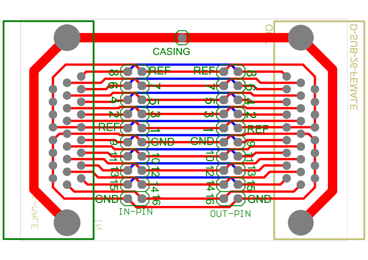
Figure 1: Schematics of the direct adapter between electrodes and amplifiers.

The EEG channels were positioned according to the 10-20 system at AFz, Fz, FCz, C3, C1, Cz, C2, C4, CPz, P3, Pz, P4, POz, O1, Oz and O2 – ground at FPz, reference on the left earlobe. Since the measures between both amplifiers were identical, only one recording session occurred, with one participant – there were no factors to counterbalance with repeated measures. The signals of both amplifier were acquired using OpenViBE 1.0.1; at 512Hz sampling rate for the g.USBamp and 125Hz sampling rate for the OpenBCI board.

The spectral features were investigated with a workload monitoring application, i.e. a BCI that is able to discriminate between several levels of mental effort. The system was trained using the N-back task, a well-known task to induce workload by playing on memory load and time pressure (see, e.g. [Mühl et al., 2014]). The protocol we used was similar to [Mühl et al., 2014], there were 360 trials presented during 6 blocks of alternate difficulty levels (0-back vs 2-back conditions). The recording session lasted approximately 12 minutes.

The temporal features were investigated using an oddball task directly implemented within OpenViBE with a visual P300 speller. P300 spellers are well-established BCI applications during which letters that randomly flash on the screen can be used to spell words with the sole brain activity. Indeed, when the letter that the user wants to spell flashes, a particular event-related potential (ERP) arises within the EEG, which possess a positive “peak” around t=300 ms after the stimulus onset. This is commonly referred to as the “oddball paradigm” since the occurrence of rare stimuli is used to elicit brain responses. During the recordings a matrix of 6 by 6 letters and digits was displayed in full screen on a 24-inch display. Only the calibration session occurred, during which one need to focus one’s attention on a predefined sequence of letters. 32 letters composing a pangram were mentally “spelled” this way. The sentence was, without spaces, “pack my box with five dozen liquor jugs”. Letters were flashing for 0.2s. There were 24 flashes per letter (12 times the row, 12 times the column), hence due to the matrix disposition there were in total 4608 trials, among which 768 were targets – “odd” trials, i.e. the letters of the target sentence were flashing. The recording session lasted approximately 30 minutes.

The acquisition of both amplifiers’ signals and the P300 application occurred within the same OpenViBE scenario (script). The recordings of each amplifier were synchronized with the appropriate events and exported in separate GDF files for later analyses. There was also only one scenario involved in the synchronization of all signals and events in the case of the N-back task; stimulation from the python script supporting this latter task were retrieved using the LSL protocol, a network protocol dedicated to physiological recordings which ensures accurate timings.

2.2 Signal processing

Two kinds of analyses were performed, using standard BCI signal processing pipelines. One aimed at assessing if and how the amplifiers differ in practice, when used for classification. The second then looked at the correlation between the acquired signals.

2.2.1 Classification

The signal processing of the data acquired during the N-back task is analogous to [Mühl et al., 2014], i.e. 2s time windows, 5 frequency bands – delta (1-3 Hz), theta (4-6 Hz), alpha (7-13 Hz), beta (14-25 Hz) and gamma (26-40 Hz) – and spatial filters. We used common spatial patterns spatial filters to reduce the 16 channels to 6 “virtual” channels more discriminant between the workload conditions – see [Ramoser et al., 2000]. Additionally, we also tested a 3 frequency bands version of our pipeline, that consider only the lower frequencies, less prone to muscular artifacts – delta, theta and alpha.

Concerning the oddball task, we band-passed the signal between 0.5Hz and 40Hz, downsampled it by a factor 32 using the “decimate” Matlab function – by a factor 8 for OpenBCI because of the reduced sampling rate –, and applied regularized Eigen Fisher spatial filters – a spatial filter specifically designed for ERPs classification [Hoffmann et al., 2006] – to reduce channels’ dimension from 16 to 5. We used 1s time windows after stimuli onsets – letters’ flashes – to epoch (“slice”) our signal. However, in order to prevent data to overlap between consecutive stimuli due to the rapid pace of the flashes, after a first pass of epoching we discarded overlapping time windows from further analyses. This ensured that no part of the signal could be seen twice by the classifier between the training phase and the testing phase and bias the accuracy. The procedure was automatic, the first non-overlapping epoch in order of appearance being kept. As a result, in the end we obtained 48 target trials and 240 distractor trials for classification, identical between the g.USBamp and the OpenBCI recordings.

Both for the workload and the P300 speller tasks, we used shrinkage LDA (linear discriminant analysis) for classification [Ledoit and Wolf, 2004]. To assess the classifiers’ performance on the calibration data, we used 4-fold cross-validation. I.e. we split the collected data into 4 parts of equal size, used 3 parts to calibrate the classifiers and tested the resulting classifiers on the unseen data from the remaining part. This process occurred 3 more times so that in the end each part was used once as test data. Finally, we averaged the obtained classification accuracies. The accuracy was measured using the area under the receiver-operating characteristic curve (AUROCC). The AUROCC is a metric that is robust against unbalanced classes, as it is the case with oddball tasks. A score of “1” means a perfect classification, a score of “0.5” is chance. In order to make statistical comparisons between both amplifiers for each type of features that we studied, we ran 10 times the analyses – the trials were selected randomly for cross-validation.

2.2.2 Correlations

We compared, on the one hand, the frequency spectra associated to the different workload conditions and, on the other hand, the time course of the ERP that were caused by the flashing target letters. To do so, we used Pearson correlations, on par with the literature for similar analyses – e.g. [Zander et al., 2011]. In order to ensure a 1-to-1 correspondence between our sets of data, the recordings from the g.USBamp were downsampled to 125Hz – same sampling rate as for the OpenBCI – using the “resample” function from Matlab R2014a signal processing toolbox.

Concerning the workload task, we first aggregated the 2s time-windows corresponding to each condition (0-back and 2-back). Then we used the “spectopo” function of the EEGLAB toolbox (version 13.4.4b) to compute the grand average power spectral between 1Hz and 40Hz, for each channel. The output of the function was then passed on to R (version 3.0.2) to compute correlations through the “rcorr” function from the “Hmisc” package.

For the oddball task, we first band-passed the signals between 1Hz and 8Hz – the approximate frequency band used for classification. Then we extracted time epochs starting 0.5s prior to the flashing of the target letters and ending 1s after stimuli onset. Contrary to what occurred for classification, we did not prune overlapping epochs in the oddball task when we compute the averaged ERP – there was no bias that could have been induced here. Finally, we averaged the ERP per channel before exporting the time points to the R environment.

2.3 Results

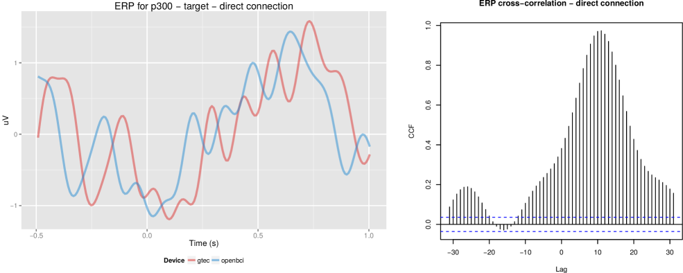
Figure 2: Left: Averaged ERP across channels of the target trials during the oddball task, before time shift correction. Right: Cross-correlation between the amplifiers. The computed lag of 11 data points corresponds to 88ms. (Direct connection.)

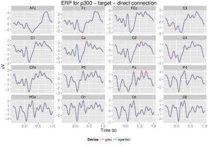
(a)

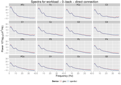
(b)

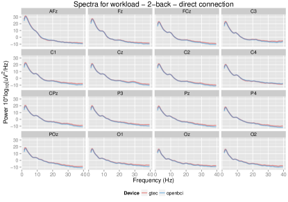
(c)

Figure 3: Direct connection: averaged ERP for the target trials of the oddball task (a), averaged spectra for the 0-back (b) and 2-back (c) trials of the N-bak task.

2.3.1 Classification

The results regarding classification accuracy are presented in Table 1, with the AUROCC scores for each one of the 10 repetitions, for both amplifiers and both tasks – including the 3 and 5 frequency bands pipeline for workload.

We tested for significance using Wilcoxon signed-rank tests. There was a significant difference between amplifiers for the P300 tasks (p < 0.01). The AUROCC mean score for the g.USBamp was 0.961 vs 0.918 for the OpenBCI. There were however no significance but tendencies concerning the workload task, with mean AUROCC scores between 0.85 and 0.86 for the 3 bands pipeline (p = 0.095) and between 0.89 and 0.90 for the 5 bands task (p = 0.079) – see Table 1 for details.

Condition	Amplifier	1	2	3	4	5	6	7	8	9	10	Mean	SD
P300	g.USBamp	0.96	0.96	0.96	0.96	0.96	0.96	0.96	0.96	0.96	0.97	0.961	0.003
	OpenBCI	0.92	0.92	0.91	0.91	0.92	0.92	0.93	0.92	0.92	0.91	0.918	0.006
WL 3b	g.USBamp	0.85	0.85	0.85	0.86	0.85	0.87	0.87	0.87	0.87	0.86	0.860	0.009
	OpenBCI	0.86	0.86	0.85	0.86	0.84	0.86	0.85	0.85	0.85	0.85	0.853	0.007
WL 5b	g.USBamp	0.90	0.89	0.90	0.89	0.91	0.90	0.89	0.90	0.89	0.90	0.897	0.007
	OpenBCI	0.91	0.89	0.87	0.88	0.89	0.88	0.89	0.89	0.89	0.90	0.889	0.011

Table 1: Classification accuracy (AUROCC scores) for the P300 and workload tasks studied during the first experiment – direct connection between the electrodes and the amplifiers. The 4-fold cross validations were repeated 10 times. Two pipelines are presented for the workload: 3 frequency bands (“WL 3b”, $\delta+\theta+\alpha$) as well as 5 frequency bands pipeline (“WL 5b”, $\delta+\theta+\alpha+\beta+\gamma$). Significance was tested using Wilcoxon signed-rank tests.

	AFz	Fz	FCz	C3	C1	Cz	C2	C4	CPz
P300 target	0.998	0.997	0.997	0.997	0.997	0.994	0.996	0.992	0.994
Workload 0-back	0.999	0.999	0.998	0.998	0.998	0.998	0.998	0.999	0.998
Workload 2-back	0.999	0.999	0.998	0.998	0.998	0.998	0.998	0.999	0.997
	P3	Pz	P4	POz	O1	Oz	O2	Mean	SD
P300 target	0.995	0.994	0.996	0.996	0.996	0.994	0.995	0.9965	0.0015
Workload 0-back	0.998	0.998	0.998	0.999	0.998	0.998	0.998	0.9983	0.0003
Workload 2-back	0.998	0.998	0.998	0.998	0.997	0.998	0.998	0.9979	0.0005

Table 2: Pearson correlation R scores between g.USBamp and OpenBCI recordings at the 16 different electrode locations with a direct connection. The “P300 target” condition corresponds to temporal features (ERP averaged across trials) and the workload conditions to spectral features.

2.3.2 Correlations

When we first analyzed our data to seek correlations regarding the oddball tasks, we realized that a shift occurred during the recordings, as denoted in Figure 2 by the grand average of the ERP for target trials across channels. This may have been caused by a software issue (see Discussion). In order to correct the shift and conduct proper comparisons between both amplifiers’ measures, we used a cross-correlation to estimate the time shift, using the “ccf” function from the R “stats” package. We found a delay of 88ms between the two signals – 11 data points at 125Hz, see Figure 2.

In Figure 3a, the averaged ERP were shifted by as much for each channel. Corresponding Pearson correlation R scores, that were computed using the “rcorr” function, are presented in Table 2. The mean R score is 0.9965 and is statistically significant (p < 0.001).

There was also a significant correlation (p < 0.001) for the spectral features, with a mean R score of 0.9983 for the 0-back condition and 0.9979 the 2-back condition (see Table 2 for details). Among the brain signals patterns that could be expected during the completion of a difficult task, the decrease nearby the alpha frequency band during the 2-task condition can be observed within per-channel spectra presented in Figures 3b and 3c. Note that we did not correct time shifts prior to workload analyses due to the nature of the features – i.e. spectral and not temporal.

2.4 Discussion

The correlation between both temporal and spectral features tends so show that the signals acquired by the g.USBamp and the OpenBCI are, if not identical, very closely related. For every condition and channel tested, the Pearson R score was greater than 0.99.

There were however more dissimilarities in the classification accuracy obtained during the corresponding tasks. While there were hardly a difference between the AUROCC scores computed from both amplifiers with the N-back tasks, the g.USBamp performed significantly better than the OpenBCI during the P300 speller task. The time shift observed afterwards between the two amplifiers may partially explain this difference. Indeed, the detection of ERP is particularly sensitive to signals’ latency, and a shift between events’ timestamp and signal’s acquisition could result in such degradation of performance when temporal features are involved.

The radio transmission between the wireless OpenBCI board and the dongle plugged to the computer may be one of the cause of the situation. The problem could also originate from the software. As a matter of fact, the OpenViBE acquisition driver of the OpenBCI board was released no so long before our experiment, and was still labelled as “unstable” as for version 1.0.1 of the software. One “oddity” that may further highlight the youth of OpenBCI software integration: we realized during our analysis that the recorded signals were completely inverted on the Y axis. The voltage reported by the board were the opposite of what g.USBamp was claiming. Since on numerous occasions we acknowledged the accuracy of g.tec devices readings, it is the OpenBCI’s signals that we inverted back to “normal” prior to correlation analyses.

Beside time shifts issues, as mentioned during the introduction we needed to strengthen those first insights by discarding the eventuality that both EEG signals may have influence each other due to the direct wiring with the electrodes.

3 SECOND EXPERIMENT: ISOLATED CONNECTIONS

The second set of recordings is very similar to the what was described during the first study. The second experiment only differs by the nature of the adapter that was employed. As such we will only discuss the changes that were made to the hardware and quickly dive into the results.

3.1 Ideal adapter

We modified the adapter that connects the amplifiers to the g.GAMMAbox – and by extent to the EEG electrodes. Instead of a direct connection between each amplifier’s inputs and the EEG channels, we interposed “ideal” (or “super”) diodes on the branches of the “Y” wiring.

Diodes are electrical components that let the current flow in only one direction, the “forward” direction. Hence, this type of montage ensures that no current could travel directly from one amplifier to the other, contaminating the recordings. However, regular diodes cause a voltage drop. The voltage drop varies depending on the materials used for their construction, but it is at least 0.3V. Meaning that if the current coming in the forward direction is lesser than 0.3V, no signal will pass through. 0.3V is an order of magnitude superior to the range of EEG signal – approximately a thousand time, therefore regular diode could not be used.

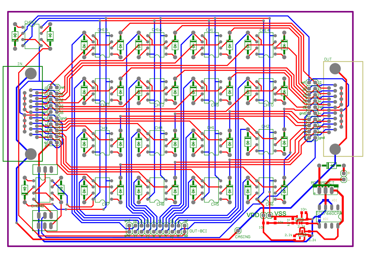
Figure 4: Schematics of the adapter with the ideal diodes montage. Note that there is a set of ideal diodes on the ground channel, but they were shorted with a jumper during our experiment.

To circumvent this problem, we utilized a particular montage that involved operational amplifiers (op-amp). Op-amps are components widely used in electrical circuits, acting as sorts of “building blocks”. Notably, in combination with a regular diode, one could use a precision rectifier configuration to obtain an “ideal” diode. This particular montage is also known as a “super” diode, since there will always be a slight voltage drop, but in this case, thanks to the gain of the op-amp, it becomes negligible.

We mounted 36 of such ideal diodes on the adapter. One on each end of the “Y” section associated to the 16 EEG channels, plus 2 for the reference. Due to the nature of the electrical recordings, only the ground was left without such circuit. We utilized Texas Instrument op-amps, model TLC2272ACPE4. The TLC227xA series are more indicated for precision application, and with 2 op-amps per chip we could limit the overall size of the adapter. The operational amplifiers were powered by an external circuit with regulated -2.5 / +2.5 voltage. The schematics of the adapter – also a 2 layers 2 layers PCB – is presented in Figure 4. The ideal diodes montage, placed before amplifiers’ inputs, prevented any current to flow in reverse direction from either amplifier to the adapter; it ensured that one set of recordings would not bias the other. One recording session occurred for each application and each condition.

3.2 Results

The signal processing and the analyses were strictly identical to the first experiment detailed above, refer to the previous section for related information.

3.2.1 Classification

As with the first study, the results regarding classification accuracy are presented in Table 3, with the AUROCC scores for each one of the 10 repetitions, for both amplifiers and both tasks – including the 3 and 5 frequency bands pipeline for workload. We tested for significance using Wilcoxon signed-rank tests. No matter the task there was no significant difference, although the 5% threshold was nearly reached for spectral features – p-value was 0.157 for the P300 task, 0.051 for the 3 bands version of the workload pipeline and 0.286 for the 5 bands version.

3.2.2 Correlations

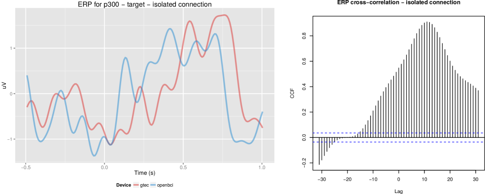
Figure 5: Left: Averaged ERP across channels of the target trials during the oddball task, before time shift correction. Right: Cross-correlation between the amplifiers. The computed lag of 11 data points corresponds to 88ms. (Isolated connection.)

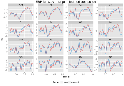
(a)

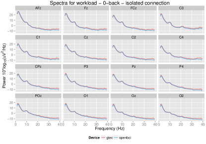
(b)

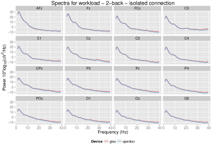
(c)

Figure 6: Isolated connection: averaged ERP for the target trials of the oddball task (a), averaged spectra for the 0-back (b) and 2-back (c) trials of the N-bak task.

Concerning the P300 oddball task, there was a offset of 88ms as well between the recordings of both amplifier with the isolated connection – see Figure 5 for the grand ERP average and the cross correlation. The per-channel averaged ERP are plotted in figure 6a. Corresponding Pearson correlation R scores are presented in Table 4. The mean R score is 0.8847 and is statistically significant (p < 0.001).

There was also a significant correlation (p < 0.001) for the spectral features, with a mean R score of 0.9976 for the 0-back condition and 0.9987 the 2-back condition (see Table 4 for details). The per-channel spectra are presented in Figures 6b and 6c. As with the direct connection, the band frequency changes between the 0-back and the 2-back conditions can be observed in the spectra.

Condition	Amplifier	1	2	3	4	5	6	7	8	9	10	Mean	SD
P300	g.USBamp	0.84	0.82	0.83	0.83	0.81	0.85	0.83	0.84	0.83	0.84	0.832	0.011
	OpenBCI	0.82	0.83	0.83	0.82	0.81	0.82	0.84	0.82	0.83	0.83	0.825	0.008
WL 3b	g.USBamp	0.88	0.88	0.88	0.91	0.89	0.90	0.89	0.88	0.89	0.88	0.888	0.100
	OpenBCI	0.88	0.88	0.89	0.89	0.88	0.89	0.87	0.88	0.88	0.87	0.881	0.007
WL 5b	g.USBamp	0.92	0.91	0.92	0.90	0.91	0.89	0.90	0.91	0.91	0.90	0.907	0.009
	OpenBCI	0.90	0.92	0.92	0.91	0.92	0.90	0.91	0.91	0.90	0.91	0.910	0.008

Table 3: Classification accuracy (AUROCC scores) for the P300 and workload tasks studied during the second experiment – isolated connection between the electrodes and the amplifiers. The 4-fold cross validations were repeated 10 times. Two pipelines are presented for the workload: 3 frequency bands (“WL 3b”, $\delta+\theta+\alpha$) as well as 5 frequency bands pipeline (“WL 5b”, $\delta+\theta+\alpha+\beta+\gamma$). Significance was tested using Wilcoxon signed-rank tests.

	AFz	Fz	FCz	C3	C1	Cz	C2	C4	CPz
P300 target	0.976	0.934	0.892	0.846	0.872	0.881	0.838	0.811	0.912
Workload 0-back	0.999	0.998	0.998	0.997	0.998	0.998	0.998	0.996	0.998
Workload 2-back	0.999	0.999	0.999	0.998	0.998	0.999	0.999	0.999	0.999
	P3	Pz	P4	POz	O1	Oz	O2	Mean	SD
P300 target	0.849	0.823	0.896	0.910	0.878	0.982	0.853	0.8847	0.0483
Workload 0-back	0.998	0.998	0.998	0.997	0.997	0.997	0.997	0.9976	0.0007
Workload 2-back	0.999	0.999	0.999	0.999	0.999	0.998	0.998	0.9987	0.0004

Table 4: Pearson correlation R scores between g.USBamp and OpenBCI recordings at the 16 different electrode locations with an isolated connection. The “P300 target” condition corresponds to temporal features (ERP averaged across trials) and the workload conditions to spectral features.

3.3 Discussion

The results with the isolated connections are not that different from what was obtained during the first experiment. This would suggest that directly connecting two high impedance amplifiers to the same EEG electrodes could be a viable montage for a side-by-side comparison.

Since with both types of connector there was only one set of recordings, we could not draw any conclusion about the lower classification accuracy obtained with the isolated montage. The vigilance level of the participant alone could explain these performances.

Thanks to signals’ correlations, however, we may infer that noise was added to the system due to the presence of additional electrical components in the adapter. Indeed, while the spectra were once again strongly correlated, the averaged ERP achieved “only” a mean R score of 0.88. Here external factors such as the metal state of the participant or the quality of electrodes contacts could not have influenced one amplifier rather than the other. Since temporal features are more sensitive than spectral features to signal quality – e.g. one “peak” in the signal vs oscillatory patterns over several seconds –, it is instead more plausible that the difference with the first experiment comes from the adapter.

Nonetheless, even though the ideal diode montage did not produce ideal signals, those results still advocate for a close proximity between the g.USBamp and the OpenBCI. No device behaved “better” than the other, because no matter the lower correlation between averaged ERP, the classification accuracy is in practice comparable between both amplifiers. Each one probably endured different fluctuations since each had a dedicated set of ideal diodes.

4 CONCLUSION

During this preliminary study, we compared the OpenBCI board to the g.tec g.USBamp amplifier. We employed an original montage, based on the simultaneous recording of the same set of electrodes. While as a first approach we used a simple adapter with a direct connection between the amplifiers and the electrodes, in a second experiment we attempted to discard any possible interference that one amplifier could cause to the other.

To do so, we built an adapter that embedded “ideal” diodes, components that prevented electrical currents to flow “backward”. This ensured that we could test both devices in isolation. We did not try to compare both adapters as the purpose was simply to gather more insights about the possibility of simultaneous recordings – this was a precaution to detect a possible bias. For all applications and conditions AUROCC scores were far beyond chancel level; the OpenBCI amplifier came close to the g.USBamp in terms EEG features and effective performance.

That is not to say that the OpenBCI could replace an equipment such as the g.USBamp, though. For instance, this open-hardware initiative does not aim at medical applications, hence it should be employed in sensitive contexts. It does not possess any certification; one reason why so many cheap EEG device are wireless is not for practicality, but to avoid any hazard due to power supply. Connecting somehow a body to the power grid requires extra precautions and a certified isolation, moreover when the impedance between the electrodes and the brain is intentionally lowered.

There are also few issues with the current state of the OpenBCI project. One concerns the sampling rate of the board. While 125Hz may be enough for our use-cases – no frequencies beyond 40Hz were used during the work presented here – it may not suffice others. The limitation of the sampling rate is caused by the wireless protocol used for data transmission. OpenBCI can deliver up to 250Hz signals to the computer, but only on 8 channels instead of 16. Note that this may be optimized in the future by updating the firmware or using alternate communications – as far as the board itself is concerned, the documentation of the ADS1299 chip ensuring analog-to-digital conversion claims a sampling rate up to 16,000Hz.

With those limitations in mind, overall the results suggest that the OpenBCI board – or a similar solution based also on the Texas Instrument ADS1299 chip – could be an alternative to traditional EEG amplifiers. Even though medical grade equipment possesses certification and still outperforms the OpenBCI board in terms of classification, the latter gives very close EEG readings. In practice, the obtained classification accuracy may be suitable for reliable BCI in popular settings, widening the realm of applications and increasing the number of potential users.

5 ACKNOWLEDGMENTS

I thank Thibault Laine for his technical assistance during this project.

REFERENCES

- [Hoffmann et al., 2006] Hoffmann, U., Vesin, J., and Ebrahimi, T. (2006). Spatial filters for the classification of event-related potentials. In ESANN ’06.
- [Ledoit and Wolf, 2004] Ledoit, O. and Wolf, M. (2004). A well-conditioned estimator for large-dimensional covariance matrices. Journal of Multivariate Analysis, 88(2):365–411.
- [Mühl et al., 2014] Mühl, C., Jeunet, C., and Lotte, F. (2014). EEG-based workload estimation across affective contexts. Frontiers in Neuroscience, 8(8 JUN):1–15.
- [Nijboer et al., 2015] Nijboer, F., van de Laar, B., Gerritsen, S., Nijholt, A., and Poel, M. (2015). Usability of Three Electroencephalogram Headsets for Brain–Computer Interfaces: A Within Subject Comparison. Interacting with Computers, 27(5):500–511.
- [Ramoser et al., 2000] Ramoser, H., Müller-Gerking, J., and Pfurtscheller, G. (2000). Optimal spatial filtering of single trial EEG during imagined hand movement. IEEE Trans Rehabil Eng, 8(4):441–446.
- [Tan and Nijholt, 2010] Tan, D. S. and Nijholt, A. (2010). Brain-Computer Interfaces: Applying Our Minds to Human-Computer Interaction. Springer.
- [Tautan et al., 2013] Tautan, A.-M., Serdijn, W., Mihajlovic, V., Grundlehner, B., and Penders, J. (2013). Framework for evaluating EEG signal quality of dry electrode recordings. 2013 IEEE Biomedical Circuits and Systems Conference (BioCAS), pages 186–189.
- [Wolpaw et al., 2002] Wolpaw, J. R., Birbaumer, N., McFarland, D. J., Pfurtscheller, G., and Vaughan, T. M. (2002). Brain-computer interfaces for communication and control. Clin. Neurophysiol., 113(6):767–91.
- [Zander and Kothe, 2011] Zander, T. O. and Kothe, C. (2011). Towards passive brain-computer interfaces: applying brain-computer interface technology to human-machine systems in general. J. Neural. Eng, 8(2):025005.
- [Zander et al., 2011] Zander, T. O., Lehne, M., Ihme, K., Jatzev, S., Correia, J., Kothe, C., Picht, B., and Nijboer, F. (2011). A Dry EEG-System for Scientific Research and Brain–Computer Interfaces. Frontiers in Neuroscience, 5(May):1–10.