TUM-HEP-1045/16
June 7, 2016

Threshold singularities, dispersion relations and
fixed-order perturbative calculations

M. Beneke and P. Ruiz-Femenía
Physik Department T31,
James-Franck-Straße, Technische Universität München,
D–85748 Garching, Germany

We show how to correctly treat threshold singularities in fixed-order perturbative calculations of the electron anomalous magnetic moment and hadronic pair production processes such as top pair production. With respect to the former, we demonstrate the equivalence of the “non-perturbative”, resummed treatment of the vacuum polarization contribution, whose spectral function exhibits bound state poles, with the fixed-order calculation by identifying a threshold localized term in the four-loop spectral function. In general, we find that a modification of the dispersion relation by threshold subtractions is required to make fixed-order calculations well-defined and provide the subtraction term. We then solve the apparent problem of a divergent convolution of the partonic cross section with the parton luminosity in the computation of the top pair production cross section starting from the fourth-order correction. We find that when the computation is performed in the usual way as an integral of real and virtual corrections over phase space at a given order in the expansion in the strong coupling, an additional contribution has to be added at N3LO.

1 Introduction

The photon vacuum polarization contribution to the electron anomalous magnetic moment $g_{e}-2$, see Figure 1 is given by [1, 2]

$$a_{e}^{\rm(vp)} =-\frac{\alpha}{\pi}\int_{0}^{1}dx\,(1-x)\,\Pi\Big{(}\frac{-x^{2}}{1-x}\,m^{2}\Big{)}\,,$$ (1)

with $\alpha$ the fine structure constant and $m$ the electron mass. Exploiting the analyticity of $\Pi(s)$ and the standard on-shell renormalization condition $\Pi(0)=0$, the once-subtracted dispersion relation

$$\Pi(q^{2}) =\frac{q^{2}}{2\pi i}\oint ds\,\frac{\Pi(s)}{s\,(s-q^{2})}=\frac{q^{2}}{\pi}\int_{0}^{\infty}\frac{ds}{s}\,\frac{{\rm Im}\,\Pi(s+i\eta)}{s-q^{2}}$$ (2)

holds, which allows us to rewrite (1) as

$$a_{e}^{\rm(vp)} =\frac{\alpha}{\pi^{2}}\int_{0}^{\infty}\frac{ds}{s}\,{\rm Im}\,\Pi(s+i\eta)\,K(s)$$ (3)

with kernel function

$$K(s) =\int_{0}^{1}dx\,\frac{x^{2}(1-x)}{x^{2}+(1-x)s/m^{2}}\;.$$ (4)

The spectral function ${\rm Im}\,\Pi(s)$ exhibits a series of positronium poles slightly below the electron-positron threshold $4m^{2}$. In [3] it has been claimed that this results in an additional ${\cal O}(\alpha^{5})$ contribution to the magnetic moment, which is not captured by the ${\cal O}(\alpha^{5})$ QED correction from the four-loop vacuum polarization function [4]. This claim has been quickly refuted [5, 6, 7] — indeed, it is clear from (1) that the vacuum polarization is probed only in the Euclidean region far from the electron-positron threshold, where an ordinary loop expansion is valid —, but the arguments presented leave an interesting point open, namely whether and how an order-by-order calculation of the spectral function gives the correct result for the magnetic moment when the dispersive representation (3) is used. The answer to this question, which we provide in this note, leads to more general considerations on the formulation of the dispersion relation for spectral functions whose perturbative expansions become more and more singular near pair-production thresholds as the order of the expansion increases. This in turn has interesting ramifications for pair production of heavy particles such as top quarks at the Large Hadron Collider as will be discussed.

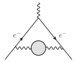
Figure 1: Vacuum polarization contribution to the anomalous magnetic moment of the electron.

2 Equivalence at ${\cal O}(\alpha^{5})$

The vacuum polarization function develops poles of $e^{+}e^{-}$ bound states right below the electron-positron threshold. They cannot be obtained at any finite order in QED perturbation theory, but arise diagrammatically from the summation of an infinite number of Coulomb-photon exchanges between the electron and positron. The systematic resummation can be performed within the framework of non-relativistic effective field theory, and the relevant counting is $v\equiv\sqrt{E/m}\sim\alpha$ with $E=\sqrt{s}-2m$.

The summation generates the bound-state poles and also significantly affects the $e^{+}e^{-}$ continuum near threshold. For the present discussion of ${\cal O}(\alpha^{5})$ effects both are adequately described by the leading-order Coulomb Green function. The photon vacuum polarization near threshold (small $E$) is given by

$$\Pi_{0}(E) =\frac{2\pi\alpha}{m^{2}}\,G_{0}(0,0;E)$$ (5)

in terms of the zero-distance Coulomb Green function [8, 9]

$$G_{0}(0,0;E) =\frac{m^{2}}{4\pi}\left[-\sqrt{-\frac{E}{m}}-\alpha\left\{-\frac{1}{4\epsilon}+\frac{1}{2}\ln\left(\frac{-4mE}{\mu^{2}}\right)-\frac{1}{2}+\gamma_{E}+\Psi(1-\lambda)\right\}\right],$$ (6)

here regulated dimensionally in $d=4-2\epsilon$ dimensions. The Coulomb Green function sums terms of order $(\alpha/v)^{n}$ to all orders in $\alpha$ through the digamma function $\Psi(1-\lambda)$, where $\lambda=\alpha/(2\sqrt{-E/m})$, and the poles of the digamma function at positive integer $\lambda$ correspond to the $S$-wave positronium bound states. The imaginary part of the Green function for real energies reads

$${\rm Im}\,G_{0}(0,0;E) =\sum_{n=1}^{\infty}\left(\frac{m\alpha}{2n}\right)^{3}\,\delta(E-E_{n})+\theta(E)\,\frac{m^{2}}{4\pi}\,\frac{\pi\alpha}{1-e^{-\frac{\pi\alpha}{v}}}\,,$$ (7)

where the second term is the continuum contribution known as the Sommerfeld factor and the positronium bound states at energies $E_{n}=-m\alpha^{2}/(4n^{2})$ are explicit in the first term. We shall now compute the contribution to the anomalous magnetic moment in two ways. First, “non-perturbative”, that is, using the all-order resummed spectral function above. Second, we show that exactly the same result can be obtained at fixed five-loop order in perturbation theory. We then explain why this implies that no additional contribution has to be added to the known result [4].

For the “non-perturbative”, resummed evaluation we multiply (7) by $2\pi\alpha/m^{2}$ and insert the result into (3), obtaining

$$a_{e}^{\rm(vp),res} =\frac{\alpha^{5}}{4\pi}\,\sum_{n=1}^{\infty}\,\frac{1}{n^{3}}\,\frac{K((2m+E_{n})^{2})}{1+E_{n}/2m}+\,\frac{\alpha^{3}}{\pi}\int_{0}^{\infty}\!\!\!dE\,\frac{K((2m+E)^{2})}{2m+E}\frac{1}{1-e^{-\frac{\pi\alpha}{\sqrt{E/m}}}}\,.$$ (8)

The first term represents the positronium contribution. At ${\cal O}(\alpha^{5})$ we can neglect the $E_{n}/m$ corrections, and the expression evaluates to $\alpha^{5}\zeta_{3}/(4\pi)\times K(4m^{2})$, where $\zeta_{k}=\sum_{n=1}^{\infty}1/n^{k}$ is the Riemann zeta function. The integral over the continuum spectral function contains lower order contributions starting from ${\cal O}(\alpha^{2})$, which are of no interest here, and is divergent at large $E$, which is an artifact, since the employed approximation to ${\rm Im}\,G_{0}$ applies only for small $E\ll m$. Subtracting the lower order contributions and applying a cut-off $E_{\rm max}=mv_{\rm max}^{2}$ to the energy integral, we are left with

$$\frac{\alpha^{3}}{\pi}\,K(4m^{2})\int_{0}^{v_{\rm max}}\!\!\!dv\,v\left(\frac{1}{1-e^{-\frac{\pi\alpha}{v}}}-\frac{v}{\pi\alpha}-\frac{1}{2}-\frac{\pi\alpha}{12v}\right)$$ (9)

Note that we are allowed and must choose $v_{\rm max}$ such that $\alpha\ll v_{\rm max}\ll 1$ in order to include the non-perturbative modification of the threshold region. It is straightforward to check that the largest contribution to the integral is ${\cal O}(\alpha^{2})$ and arises from the region $v\sim\alpha$, while for $v\gg\alpha$ the integrand behaves as $\alpha^{3}/v^{2}$ and hence the contribution from that region is at most of order $\alpha^{3}/v_{\rm max}\ll\alpha^{2}$. This allows us to set the upper integration limit $v_{\rm max}$ to infinity and to obtain the analytic result $-\alpha^{5}\zeta_{3}/(8\pi)\times K(4m^{2})$ (already given in [5]) for the above expression (9). Thus, the threshold contribution to the anomalous magnetic moment from the fourth-order vacuum polarization is

$$\big{[}a_{e}^{\rm(vp),res}\big{]}_{{\cal O}(\alpha^{5})} =\underbrace{\frac{\alpha^{5}\zeta_{3}}{4\pi}\,K(4m^{2})}_{\rm positronium\,\,poles}-\underbrace{\frac{\alpha^{5}\zeta_{3}}{8\pi}\,K(4m^{2})}_{\rm continuum}\,.$$ (10)

We now turn to the second, perturbative evaluation. The expansion of $\Pi(E)$ in $\alpha$ can be recovered by expanding $G_{0}(0,0;E)$ in $\alpha$, since the threshold approximation is sufficient for the present purpose. Up to the four-loop order, we find

$$\Pi_{0}^{\rm pert}(E)= -\frac{\alpha}{2}\,\sqrt{\frac{-E}{m}}-\frac{\alpha^{2}}{4}\bigg{(}-\frac{1}{2\epsilon}+\ln\Big{(}\frac{-4mE}{\mu^{2}}\Big{)}-1\bigg{)}+\frac{\pi^{2}\alpha^{3}}{24}\frac{1}{\sqrt{-E/m}}$$

$$-\frac{\alpha^{4}}{8}\,\frac{\zeta_{3}}{E/m}+{\cal O}(\alpha^{5})\,.$$ (11)

The ${\cal O}(\alpha^{4})$ contribution proportional to $1/E$ is particularly relevant for the present discussion. Interpreting $\Pi(E)$ as a distribution with $E\to E+i\eta$, where $\eta$ is positive-infinitesimal, this term implies a threshold-localized contribution to the four-loop spectral function given by

$$\big{[}{\rm Im}\,\Pi_{0}^{\rm pert}(E+i\eta)\big{]}_{{\cal O}(\alpha^{4})}= \;\frac{\pi\alpha^{4}\zeta_{3}}{8}\,m\delta(E)\,.$$ (12)

Using this in (3) we find that the threshold contribution to the anomalous magnetic moment from the fourth-order vacuum polarization is

$$\big{[}a_{e}^{\rm(vp),pert}\big{]}_{{\cal O}(\alpha^{5})} =\frac{\alpha^{5}\zeta_{3}}{8\pi}\,K(4m^{2})\,,$$ (13)

in precise agreement with (10). Thus we have shown that the fixed-order perturbative approximation accurately reproduces the threshold contribution of the exact spectral function including the positronium pole contribution, provided the threshold singularities of the vacuum polarization are interpreted in the distribution sense.

Let us add the following remarks. 1) The “non-perturbative” evaluation essentially coincides with the derivation in [5], but the perturbative one is different, since the $\delta(E)$ term in ${\rm Im}\,\Pi_{0}^{\rm pert}$ was not identified there. Instead, analyticity was invoked to relate the energy integral over ${\rm Im}\,G_{0}(0,0;E)$, which appears in $a_{e}^{\rm(vp)}$, to the asymptotic behaviour of $EG_{0}(0,0;E)$ at $E\to-\infty$. This step, while mathematically correct, is nevertheless physically somewhat dubious, since it should not be necessary to appeal to the behaviour of the Coulomb Green function outside its range of applicability. 2) The direct expansion in $\alpha$ of ${\rm Im}\,G_{0}$ in (7) using $\delta(E-E_{n})=\delta(E)+{\cal O}(\alpha^{2})$ would yield the wrong result, namely

$$\Big{[}\frac{2\pi\alpha}{m^{2}}\,{\rm Im}\,G_{0}^{\rm pert}(0,0;E)\Big{]}_{{\cal O}(\alpha^{4})} =\frac{\pi\alpha^{4}\zeta_{3}}{4}\,m\delta(E)\,,$$ (14)

which differs from the correct result (12) by a factor of two. One must either integrate the resummed spectral function properly or derive the perturbative spectral function from the expansion of $\Pi_{0}(E)$ in the distribution sense. 3) Although the threshold contribution (10) or (13) is non-zero, this does not imply that it has to be added to the result of [4]. In this paper $\Pi(s)$ is computed directly, and (1) is employed to obtain the anomalous magnetic moment, hence the subtlety of the threshold-localized $\delta(E)$ in term in the four-loop spectral function never arises.

3 Threshold-subtracted dispersion relations

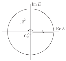
Figure 2: Integration contour defining the dispersion relation for $\Pi(E)$.

The $n$-loop vacuum polarization behaves as $\Pi^{(n)}(s)\propto\alpha^{n}E^{1-n/2}$ when $E=\sqrt{s}-2m\to 0$. The existence of non-integrable singularities at the $e^{+}e^{-}$ threshold starting at ${\cal O}(\alpha^{4})$ calls for a careful analysis of the dispersion relation (2). The first equality in (2) holds order by order, hence

$$\Pi^{(n)}(q^{2})=\frac{q^{2}}{2\pi i}\oint ds\,\frac{\Pi^{(n)}(s)}{s\,(s-q^{2})}\,.$$ (15)

The integration contour in the variable $E$ (with $s=(2m+E)^{2}$) is drawn in Figure 2. For the terms relevant in this paper the functions $\Pi^{(n)}(s)$ have a two-particle cut starting at $s=4m^{2}$, equivalently $E=0$. In order to avoid touching the singular point at $E=0$, we separate an infinitesimal circle $C_{\varepsilon}$ of radius $\varepsilon$, parametrized as $E=\varepsilon\,e^{i\varphi}$, $\varphi\in(0,2\pi)$ from the remainder of the integration contour. The straight lines above and below the cut extend from $\varepsilon$ to $+\infty$ and involve the difference $\Pi(s+i\eta)-\Pi(s-i\eta)=2i\,{\rm Im}\,\Pi(s+i\eta)$ with $\eta$ positive-infinitesimal. The circle at infinity does not contribute to the once-subtracted dispersion relation, hence (15) can be written as

$$\Pi^{(n)}(q^{2}) = \frac{q^{2}}{2\pi i}\left\{\Pi^{(n)}_{C_{\varepsilon}}(q^{2})+\Pi^{(n)}_{\rm cont}(q^{2})\right\}$$ (16)

$$= \frac{q^{2}}{\pi i}\int_{C_{\varepsilon}}\frac{dE}{2m+E}\,\frac{\Pi^{(n)}(E)}{(2m+E)^{2}-q^{2}}+\frac{2q^{2}}{\pi}\int_{\varepsilon}^{\infty}\!\frac{dE}{2m+E}\,\frac{{\rm Im}\,\Pi^{(n)}(E+i\eta)}{(2m+E)^{2}-q^{2}}\,.\qquad$$

The contribution from the small circle $C_{\varepsilon}$ vanishes for $\varepsilon\to 0$, if the vacuum polarization is less singular than $1/E$ at $E=0$; however, this condition is not satisfied in general. For the computation of the small-circle contribution $\Pi^{(n)}_{C_{\varepsilon}}(q^{2})$ we can use the expansion

$$\Pi^{(n)}(E) =\Pi^{(n)}_{0}(E)+\Pi^{(n)}_{1}(E)+\dots$$ (17)

of $\Pi^{(n)}(E)$ around threshold. The leading term, $\Pi^{(n)}_{0}(E)$, is given by the expansion in $\alpha$ of the zero-distance Coulomb Green function $G_{0}(0,0;E)$, see (5), (6) and (11). For $n\geq 3$ we have

$$\Pi_{0}^{(n)}(E)=\frac{\alpha^{2}}{2}\,\lambda^{n-2}\,\zeta_{n-1}\qquad(\lambda=\alpha/(2\sqrt{-E/m}))\,,$$ (18)

from the expansion of the Digamma function $\Psi(1-\lambda)$. The next-to-leading term $\Pi^{(n)}_{1}(E)$ is suppressed by $\sqrt{E/m}$, and equals the leading-order one times an ${\cal O}(\alpha)$ hard matching coefficient [12]:

$$\Pi^{(n)}_{1}(E) =-\frac{4\alpha}{\pi}\,\Pi^{(n-1)}_{0}(E)\,.$$ (19)

Similarly, $\Pi^{(n)}_{2}(E)$ can be extracted from the non-relativistic expansion of vacuum polarization at next-to-next-to-leading order (NNLO), and so on.

It is clear that by construction the two integrals in (16) are well-defined, but each is singular for small $\varepsilon$. We now show explicitly that the sum is well-defined in the limit $\varepsilon\to 0$. Because of the relation (19) it is sufficient to prove this for the leading term $\Pi^{(n)}_{0}(E)$ at the orders in $\alpha$ relevant to this paper. Once $\Pi^{(n)}_{2}(E)$ is included, integrals logarithmic in energy appear, but the generalization of the considerations below to this case is straightforward. Since we are only interested in the region $E\sim\varepsilon\to 0$, we can expand the denominators in the integrands of (16) in $E/m$ and $mE/(4m^{2}-q^{2})$. Then we have to prove that in the limit $\varepsilon\to 0$

$$I_{C_{\varepsilon}}^{(n,k)}(\varepsilon)+I^{(n,k)}_{\rm cont}(\varepsilon)={\cal O}(\varepsilon^{0})\;,$$ (20)

where

$$I_{C_{\varepsilon}}^{(n,k)}(\varepsilon) \equiv\frac{1}{2i}\int_{C_{\varepsilon}}\!\!dE\,E^{k}\,\Pi^{(n)}_{0}(E)\,,$$ (21)

$$I^{(n,k)}_{\rm cont}(\varepsilon) \equiv\int_{\varepsilon}^{E_{\rm max}}\!\!dE\,E^{k}\,{\rm Im}\,\Pi^{(n)}_{0}(E)\,,$$ (22)

and $k=0,1,2\dots$. We have limited the integral along the cut up to a maximum energy $E_{\rm max}$ because the expansion in $E$ potentially leads to integrands which do not converge at infinity; this is however irrelevant for the $\varepsilon\to 0$ limit studied here.

Given (18) the evaluation of the two integrals is straightforward and we find ($n\geq 3$)

$$I_{C_{\varepsilon}}^{(n,k)}(\varepsilon) =\left\{\begin{array}[]{ll}\displaystyle\frac{\alpha^{n}}{2^{n-1}}\,\zeta_{n-1}\,m^{k+1}\,\frac{\sin\frac{n\pi}{2}}{n/2-2-k}\,\Big{(}\frac{\varepsilon}{m}\Big{)}^{k+2-n/2}&\qquad k\not=\frac{n}{2}-2\\[14.22636pt] \displaystyle-\frac{\pi\alpha^{n}}{2^{n-1}}\,\zeta_{n-1}\,(-m)^{n/2-1}&\qquad k=\frac{n}{2}-2\end{array}\right.$$ (25)

and

$$I^{(n,k)}_{\rm cont}(\varepsilon) =-\frac{\alpha^{n}}{2^{n-1}}\,\zeta_{n-1}\,m^{k+1}\,\frac{\sin\frac{n\pi}{2}}{n/2-2-k}\left[\Big{(}\frac{\varepsilon}{m}\Big{)}^{k+2-n/2}\!\!\!-\Big{(}\frac{E_{\rm max}}{m}\Big{)}^{k+2-n/2}\right]\,.$$ (26)

Although we have chosen a particular form for the integration contour $C_{\varepsilon}$ surrounding $E=0$, we would get the same result (25) for any contour which has $E=\varepsilon\,e^{i2\pi^{-}}$ and $E=\varepsilon\,e^{i0^{+}}$ as initial and final points, respectively. Eqs. (25) and (26) explicitly show the cancellation of the $\varepsilon$-divergent terms between integrals $I_{C_{\varepsilon}}^{(n,k)}(\varepsilon)$ and $I^{(n,k)}_{\rm cont}(\varepsilon)$ in the dispersion relation. It is also worth noting that (26) vanishes for even $n$ and so does (25), except for the special case $k=n/2-2$ in which there is only the contribution (25) from the small circle.

We have thus shown that the dispersion relation (2) must be modified in the presence of threshold singularities. The correct dispersion relation is threshold-subtracted and reads

$$\Pi^{(n)}(q^{2})\;=\;\frac{q^{2}}{2\pi i}\,\Pi^{(n)}_{C_{\varepsilon}}(q^{2})+\frac{q^{2}}{\pi}\int_{(2m+\varepsilon)^{2}}^{\infty}\!\!ds\,\frac{{\rm Im}\,\Pi^{(n)}(s+i\eta)}{s\,(s-q^{2})}\,.$$ (27)

In the following we consider the four- and five-loop case explicitly.

The four-loop case is directly related to the discussion in section 2. For $n=4$ we must have $k=0$, and with

$$I_{C_{\varepsilon}}^{(4,0)}(\varepsilon)=\frac{\pi\alpha^{4}}{8}\,\zeta_{3}\,m\,,$$ (28)

the dispersion relation (27) for the ${\cal O}(\alpha^{4})$ vacuum polarization is

$$\Pi^{(4)}(q^{2})=\frac{q^{2}}{8\,(4m^{2}-q^{2})}\,\alpha^{4}\zeta_{3}\,+\frac{q^{2}}{\pi}\,\int_{(2m+\varepsilon)^{2}}^{\infty}\!\!ds\,\frac{{\rm Im}\,\Pi^{(4)}(s+i\eta)}{s\,(s-q^{2})}\;,$$ (29)

where we have written back the continuum integral in terms of $s$. The first term in (29) reproduces the $\alpha^{4}/E$ term in $\Pi_{0}(E)$, see (11), if we specify $q^{2}=(2m+E)^{2}$. In section 2 we interpreted this term in the distribution sense to extract its imaginary part, which then contributes to the electron anomalous moment. This contribution can now be understood as arising from an additional term in the dispersion relation obeyed by the vacuum polarization (see following section). Note that the integration over the continuum starts at $s=4m^{2}+{\cal O}(\varepsilon)$. This prevents that the contribution from the $\alpha^{4}/E$ term in $\Pi^{(4)}(E)$ could be double-counted by including its imaginary part localized at $E=0$ in the spectral density in the continuum integral.

On the other hand, for perturbative contributions to the spectral density with odd $n$, the contour integral around the threshold can be interpreted as providing the necessary subtraction terms to regulate the divergence in ${\rm Im}\,\Pi_{0}^{(n)}$ when $E\to 0$. Explicitly, at the five-loop order, where the first divergence is found, since $\Pi_{0}^{(5)}(E)\sim\alpha^{5}\,(-E/m)^{-3/2}$, the contribution from this term to the contour $C_{\varepsilon}$ reads

$$I_{C_{\varepsilon}}^{(5,k)}(\varepsilon)=\frac{\alpha^{5}}{8}\,\zeta_{4}\,m^{k+1}\,\Big{(}\frac{\varepsilon}{m}\Big{)}^{k-1/2}\,\frac{1}{1-2k}\,,$$ (30)

which is only divergent for $k=0$. At ${\cal O}(\alpha^{5})$ the NLO non-relativistic vacuum polarization $\Pi_{1}(E)$ is divergent at $E=0$ for the first time, and thus also contributes to the $C_{\varepsilon}$-contour integral. The corresponding result is simply $(-4\alpha/\pi)I_{C_{\varepsilon}}^{(4,0)}(\varepsilon)$, see (19). Plugging this together with (30) for $k=0$ into the dispersion relation (16) or (27), we obtain

$$\Pi^{(5)}(q^{2})= \ \frac{q^{2}}{2\,(4m^{2}-q^{2})}\,\frac{\alpha^{5}}{\pi}\,\left(\frac{\zeta_{4}}{4}\,\Big{(}\frac{\varepsilon}{m}\Big{)}^{-1/2}-\,\zeta_{3}\right)$$

$$+\frac{q^{2}}{\pi}\,\int_{(2m+\varepsilon)^{2}}^{\infty}\!\!ds\,\frac{{\rm Im}\,\Pi^{(5)}(s+i\eta)}{s\,(s-q^{2})}\bigg{\}}\;,$$ (31)

which, using $(\varepsilon/m)^{-1/2}=1/2\int_{\varepsilon}^{\infty}dE/m\,(E/m)^{-3/2}$, can be rewritten as

$$\Pi^{(5)}(q^{2}) = -\frac{q^{2}}{4m^{2}-q^{2}}\,\frac{\alpha^{5}}{2\pi}\,\zeta_{3}$$ (32)

$$+\,\frac{q^{2}}{\pi}\int_{(2m+\varepsilon)^{2}}^{\infty}\frac{ds}{s}\,\bigg{\{}\frac{{\rm Im}\,\Pi^{(5)}(s+i\eta)}{(s-q^{2})}+\frac{\alpha^{5}\,\zeta_{4}}{32\,(4m^{2}-q^{2})}\,\frac{\sqrt{s}}{m}\,\Big{(}\frac{m}{\sqrt{s}-2m}\Big{)}^{3/2}\bigg{\}}\,.$$

In this form of the integration over the spectral density is well-defined at the $e^{+}e^{-}$ threshold. The second term in curly brackets effectively acts as a subtraction of the divergent behaviour of the first at $s=4m^{2}$, and the $\varepsilon$ in the integration boundary is only required as a reminder that the threshold-localized $\delta(E)$ term in ${\rm Im}\,\Pi^{(5)}(s)$ should not be included.

4 Dispersive representation of $a_{e}^{\rm(vp)}$ beyond ${\cal O}(\alpha^{4})$

In this section we use the result from above to provide the corrected dispersive representation (3) for the vacuum polarization contribution to the electron anomalous magnetic moment.

At ${\cal O}(\alpha^{5})$ and ${\cal O}(\alpha^{6})$ we set $q^{2}=-x^{2}m^{2}/(1-x^{2})$ and insert the dispersion relations (29), (31) for $\Pi^{(4)}(q^{2})$ and $\Pi^{(5)}(q^{2})$, respectively, into (1). The results read

$$a_{e}^{{\rm(vp)},(5)} =\frac{\alpha^{5}}{8\pi}\,\zeta_{3}\,K(4m^{2})+\frac{\alpha}{\pi^{2}}\int_{(2m+\varepsilon)^{2}}^{\infty}\frac{ds}{s}\,{\rm Im}\,\Pi^{\rm(4)}(s+i\eta)\,K(s)$$ (33)

and

$$a_{e}^{{\rm(vp)},(6)} = -\frac{\alpha^{6}}{2\pi^{2}}\,\zeta_{3}\,K(4m^{2})$$ (34)

$$+\,\frac{\alpha}{\pi^{2}}\int_{(2m+\varepsilon)^{2}}^{\infty}\frac{ds}{s}\,\bigg{\{}{\rm Im}\,\Pi^{\rm(5)}(s+i\eta)\,K(s)+\frac{\alpha^{5}\zeta_{4}}{32}\,\frac{\sqrt{s}}{m}\,\Big{(}\frac{m}{\sqrt{s}-2m}\Big{)}^{3/2}\,K(4m^{2})\,\bigg{\}}\,.\quad$$

These two equations provide the correct expressions for the computation of the ${\cal O}(\alpha^{5})$ and (currently unknown) ${\cal O}(\alpha^{6})$ corrections to the electron anomalous magnetic moment induced by the ${\cal O}(\alpha^{4})$ and ${\cal O}(\alpha^{5})$ vacuum polarization insertions, respectively, exploiting perturbative approximations to the spectral density from $e^{+}e^{-}$ intermediate states without any resummation. In particular, the dispersive representation for $a_{e}^{{\rm(vp)},(6)}$ above is now suitable for numerical integration, since the singular $1/(\sqrt{s}-2m)^{3/2}$ behaviour of ${\rm Im}\,\Pi^{\rm(5)}$ at threshold gets cancelled by the second term. The small $\varepsilon$ dependence in the lower integration limit serves as a reminder that no imaginary part of the form $\delta(E)$ should be accounted for in the spectral density.

The dispersive representation at even higher orders in $\alpha$ can obtained in a similar way. At ${\cal O}(\alpha^{7})$ one has to consider terms arising from the NNLO non-relativistic vacuum polarization $\Pi_{2}(E)$ in the computation of $\Pi^{(n)}_{C_{\varepsilon}}(q^{2})$. Given that the calculation of the ${\cal O}(\alpha^{6})$ electron anomalous magnetic moment has not yet been attempted, it is unlikely that the expression for $a_{e}^{{\rm(vp)},(7)}$ would be needed in the foreseeable future, and we do not pursue this order further here.

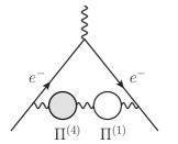
Figure 3: The relevant ${\cal O}(\alpha^{6})$ contribution with two vacuum polarization insertions. The symmetric diagram must also be considered.

Let us finally mention that at ${\cal O}(\alpha^{6})$ the dispersive representation of the diagrams with two vacuum polarization insertions also receives an additional contribution. It is easily obtained from the resummed version of (1) (see, for instance, Eq. (70) of [13]). Retaining the relevant term $2\,\Pi^{(4)}\,\Pi^{(1)}$, see Figure 3, we have

$$\delta a_{e}^{{\rm(vp)},(6)} =\frac{2\alpha}{\pi}\int_{0}^{1}dx\,(1-x)\,\Pi^{(4)}\Big{(}\frac{-x^{2}}{1-x}\,m^{2}\Big{)}\,\Pi^{(1)}\Big{(}\frac{-x^{2}}{1-x}\,m^{2}\Big{)}\;.$$ (35)

Inserting the dispersion relation (29) for $\Pi^{(4)}$ and treating $\Pi^{(1)}$ as part of a new kernel function, we obtain

$$\delta a_{e}^{{\rm(vp)},(6)}= -\frac{\alpha^{5}}{4\pi}\,\zeta_{3}\,K^{(1)}(4m^{2})-\frac{2\alpha}{\pi^{2}}\int_{(2m+\varepsilon)^{2}}^{\infty}\frac{ds}{s}\,{\rm Im}\,\Pi^{\rm(4)}(s+i\eta)\,K^{(1)}(s)\,,$$ (36)

with

$$K^{(1)}(s) \equiv\int_{0}^{1}dx\,\frac{x^{2}(1-x)}{x^{2}+(1-x)s/m^{2}}\,\Pi^{(1)}\Big{(}\frac{-x^{2}}{1-x}\,m^{2}\Big{)}\,.$$ (37)

The analytic expression for the one-loop vacuum polarization $\Pi^{(1)}(q^{2})$ can be found, for instance, in [13].

5 Hadronic pair production

Threshold singularities are also present in higher-order perturbative calculations of heavy particle pair production cross sections. The analysis of dispersion relations for the photon vacuum polarization provides the clue to solving a related divergence problem in the computation of the total pair production cross section. The following applies to any particle species (for instance, of supersymmetric particles), but we discuss it for the specific case of top quark production in hadron collisions, which is presently the most relevant one. The generalization should be evident.

The total hadronic cross section for the production of a $t\bar{t}+X$ final state in collisions of hadrons $N_{1,2}$ with centre-of-mass (cms) energy $s$ is obtained from

$$\sigma_{N_{1}N_{2}\to t\bar{t}X}(s) = \sum_{p,p^{\prime}=q,\bar{q},g}\,\int_{4m_{t}^{2}/s}^{1}\!d\tau\,L_{pp^{\prime}}(\tau,\mu_{f})\,\hat{\sigma}_{pp^{\prime}}(s\tau,\mu_{f})$$ (38)

$$= \sum_{p,p^{\prime}=q,\bar{q},g}\,\int_{0}^{\sqrt{1-4m_{t}^{2}/s}}\!\!d\beta\,L_{pp^{\prime}}(\beta,\mu_{f})\,\frac{8\beta m_{t}^{2}}{s(1-\beta^{2})^{2}}\,\hat{\sigma}_{pp^{\prime}}(\beta,\mu_{f})\,.$$

Here $\hat{\sigma}_{pp^{\prime}}(s\tau,\mu_{f})$ is the (factorization-scale dependent) partonic cross section for partonic cms energy $\hat{s}=\tau s$, $\beta=\sqrt{1-4m_{t}^{2}/\hat{s}}$, and the parton luminosity is defined in terms of the parton distributions functions (PDFs) via

$$L_{pp^{\prime}}(\tau,\mu)=\int_{0}^{1}dx_{1}dx_{2}\,\delta(x_{1}x_{2}-\tau)\,f_{p/N_{1}}(x_{1},\mu)f_{p^{\prime}/N_{2}}(x_{2},\mu)\,.$$ (39)

The parton luminosity approaches a constant near threshold $\hat{s}\to 4m_{t}^{2}$, equivalently $\beta\to 0$. The most singular behaviour of the partonic cross section is $\alpha_{s}^{2}/m_{t}^{2}\times\beta\times(\alpha_{s}/\beta)^{k}$, where in common terminology $k=1$ refers to the next-to-leading order correction to the cross section, $k=2$ to NNLO, and so on. The leading behaviour is absent for $k=3$, where instead it is given by $\alpha_{s}^{2}/m_{t}^{2}\times\beta\times(\alpha_{s}/\beta)^{2}\times\alpha_{s}\ln^{2}\beta$ [14]. Hence the convolution with the parton luminosity diverges beginning at order ${\cal O}(\alpha_{s}^{6})$ or N4LO. On the other hand, when the singular terms are summed into the Coulomb Green function, the convolution becomes convergent and the net effect of the Coulomb corrections is very small for the total cross section. These facts were noted in [14], but lead to a puzzling situation. Resummation should not be required to compute a small effect, or make the total cross section well-defined. Rather, conventional fixed-order perturbation theory should provide the correct result directly.

To approach the problem, we note that the partonic cross sections can be related to the discontinuity of the forward parton scattering amplitude

$$\hat{\sigma}_{pp^{\prime}}(\hat{s})=\frac{1}{\hat{s}}\,\mbox{Im}_{\,t\bar{t}}\,{\cal A}(pp^{\prime}\to pp^{\prime})(\hat{s})\,.$$ (40)

We then observe the similarity of the first line of (38) and the dispersive representation (3) of the vacuum polarization to the electron anomalous magnetic moment, if we identify the forward amplitude ${\cal A}_{pp^{\prime}}(\tau s)\equiv{\cal A}(pp^{\prime}\to pp^{\prime})(\tau s)$ with the vacuum polarization $\Pi(s)$, and the parton luminosity $L_{pp^{\prime}}(\tau,\mu_{f})$ with the kernel function $K(s)$. The subscript “$t\bar{t}\,$” in (40) means that only the cuts with a top-antitop pair should be included. We can ignore the other cuts, since they do not produce threshold singularities at $4m_{t}^{2}$, in the same way as the three-photon intermediate states that contribute to the photon vacuum polarization were of no relevance to the previous discussion.

The correspondence makes it clear, how the convolution (38) should be defined, at each order in perturbation theory, when the parton cross section develops non-integrable threshold singularities. We first write down the dispersion relation for ${\cal A}_{pp^{\prime}}(\hat{s})$ with a circle of infinitesimal radius around $4m_{t}^{2}$ separated, exactly as in (27). The integral term in this relation leads to (38) with the lower limit modified to $(2m_{t}+\epsilon)^{2}/s$ and a corresponding adjustment of the second line. The contribution ${\cal A}^{(n)}_{C_{\varepsilon},\,pp^{\prime}}(\hat{s})$ from the small circle has to be added as an extra contribution to the hadronic cross section. Since both terms in the subtracted dispersion relation (27) are separately divergent as $\epsilon\to 0$, it is again convenient to rewrite the circle contribution as a subtraction in the integrand of the cut contribution, similar to (31), (34). When this is done, only the threshold-localized terms in the spectral function/imaginary part of the forward amplitude remain to be added explicitly. In other words, the correct modification of (38) implies subtracting the partonic cross sections appropriately and adding the delta-function contributions.

The subtraction terms can be determined from the expansion of the forward scattering amplitude near the top threshold. It is convenient to split the production cross section into contributions from $t\bar{t}$ states in a given irreducible colour representation $R_{\alpha}$. Near threshold, the amplitude can be written in the form

$$i{\cal A}_{pp^{\prime}}^{R_{\alpha}}=\int d^{4}x\,\langle pp^{\prime}|{\mathrm{T}}[i{\cal O}_{pp^{\prime}}^{R_{\alpha}\dagger}(0)i{\cal O}_{pp^{\prime}}^{R_{\alpha}}(x)]|pp^{\prime}\rangle.$$ (41)

where ${\cal O}_{pp^{\prime}}^{R_{\alpha}}$ is a local operator, which produces a $t\bar{t}$ pair in representation $R_{\alpha}$ from the $pp^{\prime}$ parton initial state [14]. The leading term in the threshold expansion (similar to (17)) to all orders in perturbation theory reads

$$\frac{1}{\hat{s}}\,{\cal A}_{pp^{\prime},0}^{R_{\alpha}}(\hat{s})=\frac{4\pi^{2}\alpha_{s}^{2}}{m_{t}^{4}}\,\sigma_{pp^{\prime}}^{R_{\alpha}}\,G_{0}^{R_{\alpha}}(0,0;E)$$ (42)

where $G_{0}^{R_{\alpha}}(0,0;E)$ is the Coulomb Green function for the colour representation $R_{\alpha}$, given by (6) with $\alpha\to-\alpha_{s}D_{R_{\alpha}}$. The relevant cases are the attractive colour-singlet channel, $D_{1}=-C_{F}=-4/3$, and the repulsive octet one, $D_{8}=1/(2N_{c})=1/6$. The constants $\sigma_{pp^{\prime}}^{R_{\alpha}}$ can be found by comparison with the threshold-limit of the Born cross section to be

$$\sigma_{gg}^{1}=\frac{1}{96}\,,\quad\qquad\sigma_{gg}^{8}=\frac{5}{192}\,,\quad\qquad\sigma_{q\bar{q}}^{1}=0\,,\quad\qquad\sigma_{q\bar{q}}^{8}=\frac{1}{9}\,.$$ (43)

The perturbative expansion of (42) is very similar to (18).

The inclusive top pair production cross section is presently known to ${\cal O}(\alpha_{s}^{4})$ or NNLO in perturbation theory [15]. It is therefore of particular interest to investigate the implications of the above discussed modification of (38) at the next order, where indeed it arises for the first time. We recall that at this order there is no explicit divergence of the convolution integral, but since

$$\frac{1}{\hat{s}}\,{\cal A}_{pp^{\prime},0}^{R_{\alpha},(5)}(\hat{s})=-\frac{\pi\alpha_{s}^{2}}{4m_{t}^{2}}\,\sigma_{pp^{\prime}}^{R_{\alpha}}\,(-\alpha_{s}D_{R_{\alpha}})^{3}\,\frac{\zeta_{3}}{E/m_{t}}$$ (44)

causes a threshold-localized term $\delta(E)$, the threshold-subtracted dispersion relation contains a non-vanishing contribution from the circle, as in (29), (33). The result therefore reads

$$\sigma_{N_{1}N_{2}\to t\bar{t}X}^{\rm N3LO}(s) = \frac{\pi^{2}\zeta_{3}\alpha_{s}^{5}}{s}\sum_{pp^{\prime}=q\bar{q},gg}\sum_{R_{\alpha}=1,8}\,(-D_{R_{\alpha}})^{3}\sigma_{pp^{\prime}}^{R_{\alpha}}\,L_{pp^{\prime}}(4m_{t}^{2}/s,\mu_{f})$$ (45)

$$+\,\sum_{p,p^{\prime}=q,\bar{q},g}\,\int_{(2m_{t}+\varepsilon)^{2}/s}^{1}\!d\tau\,L_{pp^{\prime}}(\tau,\mu_{f})\,\hat{\sigma}_{pp^{\prime}}^{\rm N3LO}(s\tau,\mu_{f})\,.$$

If it ever becomes feasible to compute the N3LO partonic cross section $\hat{\sigma}_{pp^{\prime}}^{\rm N3LO}(\hat{s})$, it will most likely be as a sum of virtual and real contributions, integrated numerically over phase space, as presently done at NNLO [15]. In this case, the most singular behaviour would be found to be $1/\beta^{2}\times\ln^{2}\beta$ [14], but the delta-function contribution would be missed. The term in the first line of the previous equation must be added explicitly to such a computation. Numerically, however, this additional contribution is very small, as shown in Table 1. This amounts to about or less than a per mil of the total top pair production cross section, and is about an order of magnitude smaller than the cross section beyond NNLO due to the next-to-next-to-leading logarithmic (NNLL) resummation of Coulomb and soft emission effects [17].

The reason for the smallness of the additional contributions is that top pairs are predominantly produced in the colour-octet state, but the octet contribution to the first line of (45) is suppressed by $(D_{8}/D_{1})^{3}=-1/512$ due to the small colour factor. If a new species of heavy strongly interacting particles were produced in a singlet state or another colour state with a strong Coulomb interaction, no matter whether attractive or repulsive, the threshold-localized term could make a relevant contribution to the total cross section.

	Tevatron	LHC ($7\,$TeV)	LHC ($8\,$TeV)	LHC ($13\,$TeV)	LHC ($14\,$TeV)
	$\phantom{0}0.0016$	$\phantom{0}0.14$	$\phantom{0}0.19$	$\phantom{0}0.59$	$\phantom{0}0.69$

Table 1: Additional threshold-localized contribution to the inclusive N3LO top quark pair production cross section for the Tevatron $p\bar{p}$ and LHC $pp$ collider at various cms energies as given in brackets. The MSTW NNLO PDFs [16] with $\mu_{f}=m_{t}=173.3\,$GeV and $\alpha_{s}=\alpha_{s}(m_{t})=0.1085$ have been used in the evaluation. All cross sections in pb.

6 Summary

Inspired by a recent controversy over whether the positronium pole contribution needs to be added explicitly to the dispersive representation of the vacuum polarization contribution to the electron magnetic moment, we showed how this contribution is accounted for in a direct fixed-order computation. This has led us to a more general consideration of dispersion relations in the presence of a pair particle production threshold. We find that the dispersion relation requires threshold subtractions, see (27), similar to subtractions that are often required to account for the ultraviolet behaviour. The threshold-subtraction term can be determined from the expansion of vacuum polarization near the threshold. While our results imply that the dispersion relation receives additional terms, no correction of the anomalous magnetic moment is implied, since the evaluation in [4] is based on the integration of the vacuum polarization at Euclidean momenta. On the other hand, we find interesting ramifications for hadron-collider production of pairs of heavy particles, for which a Euclidean formulation is not available. When the computation is performed in the usual way as an integral of real and virtual corrections over phase space at a given order in the expansion in the strong coupling, an additional contribution has to be added at N3LO and the convolution of the partonic cross section with the parton luminosity must be modified from N4LO. We explicitly evaluated the N3LO contribution for hadronic top pair production and found that it is numerically small, of order of a per mil of the cross section.

Acknowledgements

We thank Antonio Pich for discussions on dispersion relations and Eric Laenen for comments on the manuscript. The work of MB is supported by the BMBF grant 05H15WOCAA. MB thanks the Kavli Institute for Theoretical Physics, Santa Barbara, for hospitality while this work was written up.

References

- [1] B. E. Lautrup, Nuovo Cim. A 64 (1969) 322.
- [2] B. E. Lautrup, A. Peterman and E. de Rafael, Phys. Rept. 3 (1972) 193.
- [3] G. Mishima, arXiv:1311.7109 [hep-ph].
- [4] T. Aoyama, M. Hayakawa, T. Kinoshita and M. Nio, Phys. Rev. D 83 (2011) 053003, arXiv:1012.5569 [hep-ph].
- [5] K. Melnikov, A. Vainshtein and M. Voloshin, Phys. Rev. D 90 (2014) 017301, arXiv:1402.5690 [hep-ph].
- [6] M. I. Eides, Phys. Rev. D 90 (2014) 057301, arXiv:1402.5860 [hep-ph].
- [7] M. Hayakawa, arXiv:1403.0416 [hep-ph].
- [8] D. Eiras and J. Soto, Phys. Rev. D 61 (2000) 114027, [hep-ph/9905543].
- [9] M. Beneke, Perturbative heavy quark-antiquark systems, in: Proceedings of the 8th International Symposium on Heavy Flavor Physics (Heavy Flavors 8), 25-29 July 1999, Southampton, England, [hep-ph/9911490]
- [10] M. Beneke and V. A. Smirnov, Nucl. Phys. B 522 (1998) 321, [hep-ph/9711391].
- [11] Y. Kiyo, A. Maier, P. Maierhofer and P. Marquard, Nucl. Phys. B 823 (2009) 269, arXiv:0907.2120 [hep-ph].
- [12] R. Karplus and A. Klein, Phys. Rev. 87 (1952) 848.
- [13] F. Jegerlehner and A. Nyffeler, Phys. Rept. 477 (2009) 1, arXiv:0902.3360 [hep-ph].
- [14] M. Beneke, P. Falgari, S. Klein and C. Schwinn, Nucl. Phys. B 855 (2012) 695, arXiv:1109.1536 [hep-ph].
- [15] M. Czakon, P. Fiedler and A. Mitov, Phys. Rev. Lett. 110 (2013) 252004, arXiv:1303.6254 [hep-ph].
- [16] A. D. Martin, W. J. Stirling, R. S. Thorne and G. Watt, Eur. Phys. J. C 63 (2009) 189, arXiv:0901.0002 [hep-ph].
- [17] M. Beneke, P. Falgari, S. Klein, J. Piclum, C. Schwinn, M. Ubiali and F. Yan, JHEP 1207 (2012) 194, arXiv:1206.2454 [hep-ph].