Cosmic Infrared Background anisotropies as a window into primordial non-Gaussianity

Abstract

The angular power spectrum of the cosmic infrared background (CIB) is a sensitive probe of the local primordial bispectrum. CIB measurements are integrated over a large volume so that the scale dependent bias from the primordial non-Gaussianity leaves a strong signal in the CIB power spectrum. Although galactic dust dominates over the non-Gaussian CIB signal, it is possible to mitigate the dust contamination with enough frequency channels, especially if high frequencies such as the Planck 857 GHz channel are available. We show that, in this case, measurements of the cosmic microwave background from future space missions should be able to probe the local bispectrum shape down to an amplitude $|f_{\text{NL}}|<1$.

1 Introduction

Cosmology offers powerful probes of the high-energy physics in the early Universe. One of the most important discriminants is primordial non-Gaussianity (PNG), which can in principle be tested across our entire past light-cone. While standard single-field slow-roll inflationary models generically predict only very low levels of PNG, other scenarios can lead to a much larger non-Gaussianity in the primordial fluctuations (for more details see e.g. Bartolo et al., 2004; Komatsu, 2010; Chen, 2010; Liguori et al., 2010; Yadav & Wandelt, 2010). Constraints or detections of PNG can thus give us insight into the physics at energy scales that are otherwise very difficult to access.

The Planck satellite (Planck Collaboration XVII, 2015) has already put stringent constraints on primordial non-Gaussianity, but there is still much space for interesting phenomenology, especially if we can access the regime where the amplitude of the PNG is an order of magnitude smaller than the current limits.

While the cosmic microwave background (CMB) observations are nearly cosmic-variance limited and, therefore, will not improve much over the Planck constraint, future surveys of the large scale structure (LSS) hold the promise of achieving much tighter limits. Much effort has already been devoted to constrain PNG from a scale dependence in the galaxy bias (Dalal et al., 2008; Matarrese & Verde, 2008; Slosar et al., 2008). Current LSS limits are at the level of the CMB pre–Planck constraints (Giannantonio et al., 2014; Leistedt et al., 2014), and they could improve by up to $\sim 1$ order of magnitude in the not so distant future (Agarwal et al., 2014; de Putter & Doré, 2014; Raccanelli et al., 2015; Camera et al., 2015; Alonso & Ferreira, 2015; Raccanelli et al., 2015). Further improvements may come from higher-order statistics such as the galaxy bispectrum (see e.g. Scoccimarro et al., 2004; Sefusatti & Komatsu, 2007; Jeong & Komatsu, 2009), which encodes much more information on the PNG shape than the non-Gaussian bias. The latter is predominantly sensitive to the ‘local’ bispectrum shape, which peaks on squeezed triangles.

Constraints on $f_{\text{NL}}$ from future measurements of the non-Gaussian bias will strongly depend on the survey depth and volume (Carbone et al., 2010; Hamaus et al., 2011; de Putter & Doré, 2014). Unfortunately, even the forthcoming large scale surveys such as Euclid (Laureijs et al., 2011) or LSST (Abell et al., 2009) will only cover a small fraction of the total comoving volume accessible to us. The cosmic infrared background (CIB) traces the LSS over a much larger comoving volume and, thus, could potentially outperform future galaxy redshift surveys. In this paper we show that the CIB indeed is an excellent probe of primordial non-Gaussianity that allows us, in principle, to reach $|f_{\text{NL}}|<1$ in the squeezed bispectrum limit. We demonstrate that such an error can be achieved at Fisher matrix level even upon taking into account the signal produced by galactic dust, which is much stronger than the CIB at low multipoles. However, it is essential to have CIB maps available at enough frequencies.

The paper is organized as follows. We introduce our halo model of the CIB in §2, and present our forecast for a detection of the non-Gaussian bias in the CIB angular power spectrum in §3. We discuss our findings and, in particular, the contamination by galactic dust in §4 and §5 before concluding in §6. Throughout the paper, we adopt the standard $\Lambda$CDM cosmological model as measured by Planck (Planck Collaboration XVI, 2014): $\{\Omega_{m},\Omega_{\Lambda},\Omega_{b}h^{2},\sigma_{8},h,n_{s}\}=\{0.3183,0.6817,0.02205,0.8347,0.6704,0.9619\}$.

2 Model of the Cosmic Infrared Background

2.1 Halo model of the CIB intensity

In the usual Newtonian treatment, the observed CIB brightness is given by

$$I(\nu,\mathrm{\hat{\textbf{\em n}}})=\int_{0}^{\chi_{*}}\!\!{\rm d}z\left(\frac{{\rm d}\chi}{{\rm d}z}\right)\,W_{\nu}^{({\mathtt{CIB}})}(z)\,\Big{(}1+\delta_{\jmath}\Big{)}$$ (1)

where the integral runs over the (unperturbed) comoving distance $\chi$ along the line of sight. It is typically computed up to redshift $z_{*}\sim 10$, corresponding to a comoving distance $\chi_{*}=\chi(z_{*})$, because of the negligible contribution of CIB fluctuations at higher redshifts. The redshift weight for CIB fluctuations is

$$W_{\nu}^{({\mathtt{CIB}})}(z)=a(z)\,\bar{\jmath}_{\nu}(z)\;,$$ (2)

where $a(z)$ is the scale factor and $\bar{\jmath}_{\nu}(z)$ is the mean CIB emissivity per comoving volume at frequency $\nu$:

$$\bar{\jmath}_{\nu}(z)=\int_{0}^{\bar{L}_{{}_{(1+z)\nu}}^{\text{\tiny cut}}}\!\!{\rm d}L\,\bar{n}_{g}(L,z)\,\frac{L_{(1+z)\nu}}{4\pi}\;.$$ (3)

Here, $\bar{n}_{g}(L,z)$ denotes the infrared galaxy luminosity function and $L_{(1+z)\nu}$ is the infrared luminosity (in W Hz^-1) at the rest–frame frequency $(1+z)\nu$. In practice, only faint sources below the flux detection limit $S_{\nu}^{\text{\tiny cut}}$ are included in the CIB, such that the integral in Eq. (3) is cut off at a (redshift and frequency dependent) luminosity $\bar{L}_{{}_{(1+z)\nu}}^{\text{\tiny cut}}(z)$. The brighter sources are detected and removed from the sky maps. Finally, $\delta_{\jmath}\equiv\delta_{\jmath}(\nu,z,\textbf{\em x}=\chi(z)\mathrm{\hat{\textbf{\em n}}})$ is the perturbation to the CIB emissivity at frequency $\nu$, redshift $z$ and comoving position $\textbf{\em x}=\chi(z)\mathrm{\hat{\textbf{\em n}}}$ along the line of sight.

Let us focus first on the contribution from the average emissivity. Following Shang et al. (2012), we split the mean emissivity into a sum of two contributions,

$$\bar{\jmath}_{\nu}(z)=\int\!\!{\rm d}M\,\bar{n}_{h}(M,z)\Bigl{[}f_{\nu}^{\text{c}}(M,z)+f_{\nu}^{\text{s}}(M,z)\Bigr{]}\;,$$ (4)

where the average emissivity produced by the central and satellite galaxies of a given halo at redshift $z$ are

$$f_{\nu}^{\text{c}}(M,z) =\frac{1}{4\pi}N_{\text{c}}L_{\text{c},(1+z)\nu}(M,z)$$ (5)

$$f_{\nu}^{\text{s}}(M,z) =\frac{1}{4\pi}\int\!\!{\rm d}m\,\bar{n}_{s}(m,z|M)L_{\text{s},(1+z)\nu}(m,z)\;.$$ (6)

In the above expressions, $\bar{n}_{h}(M,z)$ and $\bar{n}_{s}(m,z|M)$ are the halo and sub-halo mass functions, and $M$ and $m$ are the parent halo and sub-halo masses. The numbers $N_{\rm c}$ of central galaxies is specified by the halo occupation distribution (HOD; Berlind & Weinberg, 2002; Zheng et al., 2005). Numerical simulations indicate that $N_{\rm c}$ typically follows a step-like function (Kravtsov et al., 2004). We adopt a characteristic mass $M_{\text{cen}}$ of the step function of $3\times 10^{11}\ {\rm M_{\odot}/{\it h}}$ (Zehavi et al., 2011; Desjacques et al., 2015), ignoring any luminosity dependence. In all subsequent calculations, we use the SO (Spherical Overdensity) halo and sub-halo mass functions provided by Tinker et al. (2008) and Tinker & Wetzel (2010), respectively, and integrate the sub-halo mass function from a minimum halo mass $M_{\text{min}}=10^{10}\ {\rm M_{\odot}/{\it h}}$ to the parent halo mass $M$. To identify halos, we adopt a density threshold of $\Delta_{c}=200$ (in unit of the background density $\bar{\rho}_{m}(z)$) at all redshifts.

In the model used here, the luminosity and clustering of infrared galaxies are linked to the host halo mass. The strongly clustered galaxies are situated in more massive halos. They typically have more stellar mass and, therefore, are more luminous. Assuming the same luminosity-mass relation for both central and satellite galaxies, we relate the galaxy infrared luminosity to the host halo mass through the parametric relation (Shang et al., 2012)

$$L_{(1+z)\nu}(M,z)=L_{0}\Phi(z)\Sigma(M)\Theta_{\mathtt{CIB}}[(1+z)\nu]\,.$$ (7)

As regards to the luminosity–mass relation, we shall follow the assumptions used in Planck Collaboration XXX (2014):

• $L_{0}$ is an overall normalisation that is constrained from measurements of CIB power spectra. In principle, it should be a constant but, in order to have a good fit to Planck Collaboration XXX (2014), we allow small variations of $L_{0}$ with the frequency, which are at most a 10 per cent between 217 and 857 GHz.

• The term $\Phi(z)$ describes the redshift-dependence of the normalisation. We adopt a power-law scaling

  $$\Phi(z)=(1+z)^{\delta}.$$

• We assume a log-normal distribution for the dependence $\Sigma(M)$ of the galaxy luminosity on halo mass:

  $$\Sigma(M)=\frac{M}{\sqrt{2\pi\sigma^{2}_{\text{L/M}}}}e^{-[\log(M)-\log(M_{\text{eff}})]^{2}/2\sigma^{2}_{\text{L/M}}}\,,$$ (8)

  where $M_{\text{eff}}$ characterises the peak of the specific IR emissivity and $\sigma_{\text{M/L}}$ describes the range of halo masses that produces a given luminosity $L$, which is fixed to $\sigma^{2}_{\text{M/L}}=0.5$.

• For the galaxy spectral energy distribution (SED), we assume a modified blackbody shape with a power-law emissivity as in Hall et al. (2010),

  $$\Theta_{\mathtt{CIB}}(\nu)=\left\{\begin{array}[]{cc}(\nu/\nu_{0})^{\beta}B_{\nu}(T_{d})/B_{\nu_{0}}(T_{d})&\nu\leq\nu_{b}\\ (\nu/\nu_{0})^{-\gamma}&\nu>\nu_{b}\end{array}\right.\;,$$ (9)

  where $B_{\nu}(T)$ is the brightness of a blackbody with temperature $T$ at the frequency $\nu$, and $\nu_{0}$ is a reference frequency. The dust temperature $T_{d}$ is assumed to be a function of redshift according to $T_{d}=T_{0}(1+z)^{\alpha}$. The grey-body and power-law connect smoothly at the frequency $\nu_{b}$, at which the condition ${\rm d}{\rm ln}\Theta(\nu,z)/{\rm d}{\rm ln}\nu=-\gamma$ is satisfied. For our fiducial parameters, $\nu_{b}$ is always larger than 3000 GHz, and hence the parameter $\gamma$ has small relevance in the frequency range we are interested in.

For our fiducial halo model parameters, we adopt the values found in Planck Collaboration XXX (2014) by fitting (auto– and cross–) power spectra of the CIB anisotropies measured by Planck and IRAS at 217, 353, 545, 857 and 3000 GHz (see Table 1).

Table 1: Fiducial values of the parameters foud by Planck Collaboration XXX (2014) for the luminosity-mass relation of the halo model.

$\alpha$	T0	$\beta$	$\gamma$	$\delta$	$\log(M_{\text{eff}})$	L0
	[K]				[M⊙]	[W Hz-1]
0.36	24.4	1.75	1.7	3.6	12.6	0.95–1.05$\times 10^{-3}$

We now turn to the fluctuations of the CIB brightness across the sky. In the Limber approximation, the angular power spectrum of CIB fluctuations can be written as (e.g., Knox et al., 2001; Song et al., 2003):

$$C_{\ell}^{({\mathtt{CIB}})}(\nu,\nu^{\prime}) =\int_{0}^{z_{*}}\!\!{\rm d}z\left(\frac{{\rm d}\chi}{{\rm d}z}\right)\frac{1}{\chi^{2}}\,W_{\nu}^{({\mathtt{CIB}})}(z)W_{\nu^{\prime}}^{({\mathtt{CIB}})}(z)$$

$$\qquad\times P^{\nu\times\nu^{\prime}}_{jj}\!\!\left(k=\frac{\ell}{\chi},z\right)\,.$$ (10)

Here, $P_{jj}^{\nu\times\nu^{\prime}}$ is the cross-power spectrum $\left\langle\delta_{\jmath}\delta_{\jmath}^{\prime}\right\rangle$ of fluctuations in emissivity at frequency $\nu$ and $\nu^{\prime}$. $P_{jj}(k,z)$ can be set equal to the 3D power spectrum of galaxies, $P_{\rm gg}(k,z)$, under the assumption that fluctuations in the emissivity trace those of the sources. In the context of the halo model (Scherrer & Bertschinger, 1991; Seljak, 2000; Scoccimarro et al., 2001; Cooray & Sheth, 2002), galaxy power spectra are the sum of the contribution of the clustering in one single halo (1–halo term) and in two different halos (2–halo term):

$$P^{\nu\times\nu^{\prime}}_{\rm gg}(k,z)=\bigg{.}P_{\rm gg}^{1h}(k,z,\nu,\nu^{\prime})+P_{\rm gg}^{2h}(k,z,\nu,\nu^{\prime})\,,$$ (11)

where

$$P_{\rm gg}^{1h}(k,z,\nu,\nu^{\prime}) =\bigg{.}\frac{1}{\bar{j}_{\nu}\bar{j}_{\nu^{\prime}}}\int\!\!{\rm d}M\,\frac{{\rm d}N}{{\rm d}M}\Bigl{[}f_{\nu}^{\text{c}}(M,z)f_{\nu^{\prime}}^{\text{s}}(M,z)u(k,z|M)$$

$$\qquad+f_{\nu^{\prime}}^{\text{c}}(M,z)f_{\nu}^{\text{s}}(M,z)u(k,z|M)$$

$$\qquad+f_{\nu}^{\text{s}}(M,z)f_{\nu^{\prime}}^{\text{s}}(M,z)u^{2}(k,z|M)\Bigr{]}\,,$$

$$P_{\rm gg}^{2h}(k,z,\nu,\nu^{\prime}) =\bigg{.}\frac{1}{\bar{j}_{\nu}\bar{j}_{\nu^{\prime}}}D_{\nu}(k,z)D_{\nu^{\prime}}(k,z)P_{\text{lin}}(k,z)\,,$$ (12)

and

$$D_{\nu}(k,z) =\int\!\!{\rm d}M\,\frac{{\rm d}N}{{\rm d}M}\,b_{1}(M,z)u(k,z|M)$$ (13)

$$\qquad\times\Bigl{[}f_{\nu}^{\text{c}}(M,z)+f_{\nu}^{\text{s}}(M,z)\Bigr{]}\,.$$

Here, $u(k,z|M)$ is the normalised Fourier transform of the NFW density profile (Navarro et al., 1997), $P_{\text{lin}}(k,z)$ is the linear mass power spectrum extrapolated to redshift $z$, and $b_{1}$ is the (Eulerian) linear halo bias (we use the fitting formula given in Tinker et al., 2010). In principle, $P_{jj}(k,z)$ receives also a shot noise contribution, but we will ignore it as it is typically of the same order as the 1-halo term.

At very large scales, i.e. at multipole $\ell~{}\hbox to0.0pt{$<$\hss}{\lower 4.30554pt\hbox{$\sim$}}10$, the Limber approximation used in Eq. (10) is not valid. Assuming a negligible contribution from the 1–halo term, for angular scales ranging from $\ell=2$ to 40 CIB power spectra can be computed by (Curto et al., 2015)

$$C^{({\mathtt{CIB}})}_{\ell}( \nu,\nu^{\prime})=\frac{2}{\pi}\int\!\!{\rm d}k\,k^{2}$$ (14)

$$\times\int_{0}^{z_{*}}\!\!{\rm d}z\left(\frac{{\rm d}\chi}{{\rm d}z}\right)\,W_{\nu}^{({\mathtt{CIB}})}(z)j_{\ell}(k\chi(z))P^{1/2}_{\rm gg}(k,z,\nu)$$

$$\times\int_{0}^{z_{*}}\!\!{\rm d}z^{\prime}\left(\frac{{\rm d}\chi}{{\rm d}z}\right)\,W_{\nu^{\prime}}^{({\mathtt{CIB}})}(z^{\prime})j_{\ell}(k\chi(z^{\prime}))P^{1/2}_{\rm gg}(k,z^{\prime},\nu^{\prime})\,,$$

where $j_{\ell}(x)$ are spherical Bessel functions.

2.2 GR corrections and non-Gaussian bias

There are two important ingredients which we wish to add to the above model: General relativistic corrections and non-Gaussian bias. Details about the calculation of the GR effects, which have already been considered in the context of intensity mapping by Hall et al. (2013); Alonso et al. (2015), can be found in Appendix §A.2.

At first order in GR perturbations, the observed CIB specific intensity Eq. (1) eventually reduces to

$$I(\nu,\mathrm{\hat{\textbf{\em n}}}) =\int_{0}^{\chi_{*}}\!\!{\rm d}z\left(\frac{{\rm d}\chi}{{\rm d}z}\right)\,W_{\nu}^{({\mathtt{CIB}})}(z)$$ (15)

$$\qquad\times\bigg{(}1+\delta_{\jmath}+\frac{\partial{\rm ln}\bar{\jmath}_{\nu}}{\partial\eta}\delta\eta+\delta_{\parallel}+2\,s\,\delta_{\perp}\bigg{)}\;,$$

where $\delta_{\jmath}$ is the perturbation to the galaxy emissivity in the source rest-frame and at constant line-of-sight comoving distance $\chi$, the term proportional to $\delta\eta$ arises from the transformation to constant observed redshift, $\delta_{\parallel}$ is the perturbation to the source volume along the line-of-sight, and the term proportional to $\delta_{\perp}$ represents the perturbation to the limiting luminosity generated by fluctuations in the luminosity distance. Note that we have introduced a magnification bias

$$s(z)=\frac{\partial{\rm ln}\bar{\jmath}_{\nu}}{\partial{\bar{L}}_{{}_{(1+z)\nu}}^{\text{\tiny cut}}}=\frac{{\bar{L}}_{{}_{(1+z)\nu}}^{\text{\tiny cut}}}{4\pi}\frac{\bar{n}_{g}}{\bar{\jmath}_{\nu}}$$ (16)

in analogy with source number counts (Broadhurst et al., 1995). The mean comoving emissivity $\bar{\jmath}_{\nu}$ is given by Eq. (3). In the conformal Newtonian gauge adopted for the calculation, the perturbation to the conformal time $\eta$ reads

$${\cal H}\delta\eta=-\Psi-\int_{0}^{\chi}\!\!{\rm d}\chi^{\prime}\,\big{(}\dot{\Psi}+\dot{\Phi}\big{)}+\textbf{\em v}\cdot\mathrm{\hat{\textbf{\em n}}}$$ (17)

while the perturbations to the source volume element parallel and transverse to the beam are

$$\delta_{\parallel} =\bigg{(}{\cal H}-\frac{\dot{\cal H}}{\cal H}\bigg{)}\delta\eta+\Psi+\textbf{\em v}\cdot\mathrm{\hat{\textbf{\em n}}}$$ (18)

$$\qquad+\frac{1}{\cal H}\bigg{[}\frac{{\rm d}\Psi}{{\rm d}\chi}+\big{(}\dot{\Psi}+\dot{\Phi}\big{)}-\frac{{\rm d}\textbf{\em v}}{{\rm d}\chi}\cdot\mathrm{\hat{\textbf{\em n}}}\bigg{]}\;,$$

and

$$\delta_{\perp}={\cal H}\delta\eta-\frac{1}{\chi}\left[\delta\eta-\int_{0}^{\chi}\!\!{\rm d}\chi^{\prime}\,\big{(}\Psi+\Phi\big{)}\right]-\Phi-\kappa\;,$$ (19)

respectively. Here, overdots designate a partial derivative w.r.t. the unperturbed conformal time $\eta$. Note that $\chi$ and $\eta$ are related through $\chi=\eta_{0}-\eta$. Furthermore,

$$\kappa=\frac{1}{2}\int_{0}^{\chi}\!\!{\rm d}\chi^{\prime}\,\frac{\chi-\chi^{\prime}}{\chi\chi^{\prime}}\nabla_{\Omega}^{2}\big{(}\Psi+\Phi\big{)}\;,$$ (20)

where $\nabla_{\Omega}^{2}$ is the Laplacian on the unit sphere, is the lensing convergence. We have restricted ourselves to adiabatic scalar perturbations. There would be more terms, should vector or tensor perturbations or isocurvature modes be present at an appreciable level.

Assuming that spatial variations in the comoving emissivity trace fluctuations in the galaxy number density, intrinsic perturbations to the comoving emissivity $\delta_{\jmath}$ in the Newtonian gauge are related to matter fluctuations $\delta_{m}^{\text{\tiny syn}}$ in a synchronous gauge comoving with dark matter through (Challinor & Lewis, 2011; Baldauf et al., 2011; Jeong et al., 2012)

$$\delta_{\jmath}=b_{1}\,\delta_{m}^{\text{\tiny syn}}+\frac{\partial\,{\rm ln}\,\bar{\jmath}_{\nu}}{\partial\eta}\frac{v}{k}\;,$$ (21)

where $b_{1}(k)=b_{1}^{\text{\tiny G}}(k)+\Delta b_{1}^{\text{\tiny NG}}(k)$ is the linear galaxy bias. We have written $b_{1}(k)$ as generally the sum of a Gaussian piece $b_{1}^{\text{\tiny G}}(k)$ (which, in the halo model, depends on wavenumber through the profile $u(k,z|M)$) and a scale-dependent correction $\Delta b_{1}^{\text{\tiny NG}}(k)$ induced by the primordial non-Gaussianity. Furthermore, $v$ is a scalar function such that the (curl-free) velocity perturbation is $\textbf{\em v}=k^{-1}\textbf{\em$\nabla$}v$ in the Newtonian gauge. Finally, we have ignored the shot-noise contribution for the reasons stated above. Note that Eq. (21) is linear and, thus, corresponds to our halo bias $b(M,z)$ in Eq. (13).

To relate the perturbations $\Psi$, $\Phi$, $\delta_{m}^{\text{\tiny syn}}$ and $v$ to the initial conditions, we use $\Phi_{i}(\textbf{\em k})=(3/5)\zeta(\textbf{\em k})$, where $\zeta(\textbf{\em k})$ is the uniform-density gauge curvature perturbation on super-horizon scales (i.e. $k\ll{\cal H}$), as a reference. Our choice follows from the fact that, in the large scale structure literature, the primordial non-Gaussianity is commonly laid down immediately after matter-radiation equality (see, e.g., Desjacques & Seljak, 2010, for a review), whence the factor of $3/5$. The various transfer functions will generally depend on the matter content of the Universe. Ignoring anisotropic stresses, these are given by

$$T_{\Psi}(k,z) =\bigg{.}g(z)T(k)$$ (22)

$$T_{\Phi}(k,z) =\bigg{.}T_{\Psi}(k,z)$$

$$T_{\delta}(k,z) =\frac{2}{3\Omega_{m}}\bigg{(}\frac{k}{{\cal H}_{0}}\bigg{)}^{2}T(k)D(z)$$

$$T_{v}(k,z) =\bigg{.}\left(\frac{{\cal H}}{k}\right)f\,T_{\delta}(k,z)\;.$$

Here and henceforth, $g(z)$ and $D(z)=a(z)g(z)$ are the growth function of potential and density perturbations, respectively, $f$ is the logarithmic derivative $f=d{\rm ln}D/d{\rm ln}a$ and the matter transfer function $T(k)$ is obtained with the Boltzmann code CAMB in a synchronous gauge comoving with the pressureless matter. Note that, with our definitions, the Fourier modes of the peculiar velocity v are given by $\textbf{\em v}(\textbf{\em k},z)=i\textbf{\em k}{\cal H}fT_{\delta}(k,z)\Phi_{i}(\textbf{\em k})/k^{2}$.

Non-Gaussianity generated outside the horizon induces a 3-point function that is peaked on squeezed or collapsed triangles for realistic values of the scalar spectral index. The resulting non-Gaussianity depends only on the local value of the curvature perturbation, and can thus be conveniently parameterized by $\Phi_{i}=\phi+f_{\text{NL}}(\phi^{2}-\langle\phi^{2}\rangle)$, where $\phi$ denotes a Gaussian field (Salopek & Bond, 1990; Gangui et al., 1994). The quadratic term introduces a coupling between short- and long-wavelength modes, which results in a scale-dependent halo bias at large scales (Dalal et al., 2008; Matarrese & Verde, 2008). This non-Gaussian bias takes the form (Slosar et al., 2008)

$$\Delta b_{1}^{\text{\tiny NG}}(k,z)=3f_{\text{NL}}\left(\frac{\partial{\rm ln}\bar{n}_{h}}{\partial{\rm ln}\sigma_{8}}\right)\frac{\Omega_{m}{\cal H}_{0}^{2}}{a(z)\,T_{\Phi}(k,z)k^{2}}\;.$$ (23)

It is this bias enhancement on large scales that we are trying to measure with the CIB. A large, potentially detectable $f_{\text{NL}}\gtrsim 1$ can be produced e.g. by multiple scalar fields (Linde & Mukhanov, 1997; Lyth et al., 2003).

We have assumed that the halo mass function is universal and, thus, replaced the logarithmic derivative of the mass function by $\delta_{c}(b_{1}(M,z)-1)$, where $\delta_{c}\sim 1.68$ is the present-day (linear) critical density threshold. For the linear Gaussian bias, we use the fitting formula given in Tinker et al. (2010).

Departure from Statistical Gaussianity in the initial conditions significantly affect the abundance of highly biased tracers of the LSS, since their frequency sensitively depends on the tail of the density PDF (e.g. Lucchin & Matarrese, 1988). To ascertain the importance of this effect, we have replaced the halo mass function in Eq. (4) by

$$\bar{n}_{h}(M,z,f_{\text{NL}})=\bar{n}_{h}^{\text{\tiny G}}(M,z)\Big{(}1+R(M,z,f_{\text{NL}})\Big{)}\;,$$ (24)

where $\bar{n}_{h}^{\text{\tiny G}}(M,z)$ is our fiducial Gaussian, Tinker mass function and $R(M,z,f_{\text{NL}})$ is the non-Gaussian fractional correction modelled along the extensions proposed by Matarrese et al. (2000); Lo Verde et al. (2008) (see Desjacques & Seljak (2010) for a discussion). We have found that, for an input value $f_{\text{NL}}=1$, including $R(M,z,f_{\text{NL}})$ amounts to a $\sim 1$% correction to the amplitude of the non-Gaussian CIB bias. We will thus ignore this effect in what follows.

2.3 Signature of PNG in the CIB anisotropies

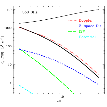
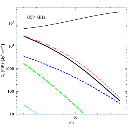
Figure 1: GR corrections (solid thick lines) to the CIB power spectrum (solid thin lines) at 353 (left panel) and 857 GHz (right panel). The different GR contributions are also isolated: the velocity term (dotted red lines); the redshift–space distorsion (short dashed blue lines); the ISW term (long dashed green term); the potential term (dot–dashed cyan lines). The GR corrections are relevant at the very first multipoles, and become lower than 1 per cent at $\ell>10$. The dominant contribution comes from the velocity term.

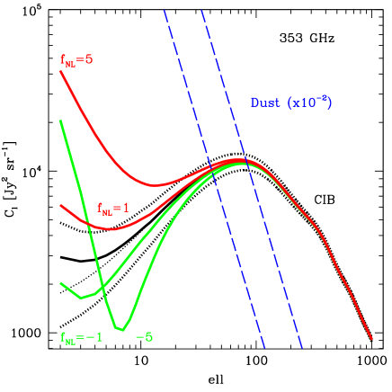
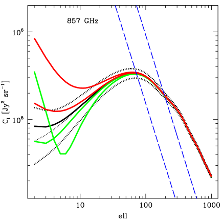
Figure 2: CIB power spectra (including GR corrections) at 353 and 857 GHz assuming Gaussian primordial fluctuations (black solid lines) and $f_{\text{NL}}=\pm 1$ and $\pm 5$ (solid red and green lines). The two, upper and lower thick dotted lines indicate the cosmic variance associated to the Gaussian case, whereas the median, thin dotted curve is the CIB power spectrum without the GR corrections. Also shown as blue dashed line is the dust contamination – reduced by a factor 100 – as measured by Planck Collaboration XXII (2015) for the cleanest sky patches with coverage fraction 10 (left line) and 40 per cent (right line). The dust contamination is still orders of magnitude larger than CIB fluctuations on large angular scales. At $\ell=2$ the CIB spectrum increases by about an order of magnitude as we turn on $f_{\text{NL}}$ from 0 to $\pm 5$. At larger multipoles, the effect of non–Gaussianity quickly decreases, and it is lower than cosmic variance at $\ell\gtrsim 20$ even for $f_{\text{NL}}\sim 5$. For negative values of $f_{\text{NL}}$, the CIB power spectrum presents a minimum at $\ell~{}\hbox to0.0pt{$<$\hss}{\lower 4.30554pt\hbox{$\sim$}}10$ corresponding to the angular scale at which the NG bias contribution becomes dominant over the Gaussian bias term.

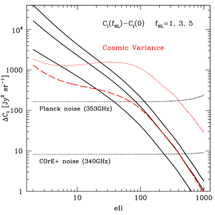
Figure 3: The cosmic variance associated to the CIB power spectrum with Gaussian initial conditions at 353 GHz (red dotted line) is shown in comparison with the PNG signal $\Delta C_{\ell}=C_{\ell}(f_{\text{NL}})-C_{\ell}(0)$ for $f_{\text{NL}}=1$, 3 and 5 (black solid lines). The red dashed line gives the cosmic variance reduced by a factor $\sqrt{\ell}$, corresponding to power spectra binned in multipole intervals of size $\ell$. The cosmic variance becomes lower than $\Delta C_{\ell}$ at $\ell~{}\hbox to0.0pt{$<$\hss}{\lower 4.30554pt\hbox{$\sim$}}20$ for $f_{\text{NL}}=1$ and lower or equal to $\Delta C_{\ell}$ up to $\ell\ga 1000$ for $f_{\text{NL}}=3$. We also plot the noise level for the Planck and COrE+ channels at $\nu\sim 350\,$GHz (black dotted lines).

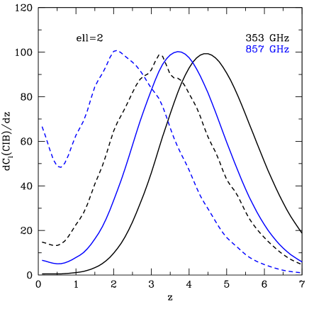
Figure 4: The redshift kernel for the CIB power spectrum at $\ell=2$ for two different frequencies: 353 GHz (black lines) and 857 GHz (blue lines). Dashed lines are for Gaussian primordial fluctuations, whereas solid lines assume local PNG with $f_{\text{NL}}=5$. CIB anisotropies induced by PNG mainly arise from dusty galaxies at redshifts between $2.5~{}\hbox to0.0pt{$<$\hss}{\lower 4.30554pt\hbox{$\sim$}}z~{}\hbox to0.0pt{$<$\hss}{\lower 4.30554pt\hbox{$\sim$}}6$ with a mild dependence on frequency.

The signature imprinted by the scale-dependent, non-Gaussian halo bias is largest at low multipoles where the contribution of the 1-halo term is negligible. We have indeed checked that, for the frequencies considered in our forecast, the 1-halo term is at most $\lesssim 10$% of the 2-halo contribution. This corresponds to an effective nonlinear parameter $|f_{\text{NL}}|\lesssim 0.1$, which is hardly accessible to CMB experiments with the sensitivity considered here. Therefore, we can safely neglect it at the low multipoles $\ell\leq 40$ where Eq. (14) is applied. Notwithstanding, we include it at the higher multipoles used to constrain the CIB model parameters since it dominates over the 2-halo term for $\ell\gtrsim 1000$.

At low multipoles $\ell\lesssim 40$ where the Limber approximation is not valid, we ignore the 1-halo term, but retain the GR corrections and the non-Gaussian bias so that the CIB angular power spectrum is computed as

$$C^{({\mathtt{CIB}})}_{\ell}( \nu,\nu^{\prime})=\frac{2}{\pi}\int\!\!{\rm d}k\,k^{2}$$ (25)

$$\times\int_{0}^{z_{*}}\!\!{\rm d}z\left(\frac{{\rm d}\chi}{{\rm d}z}\right)\,W_{\nu}^{({\mathtt{CIB}})}\!(z)F_{\ell}(\nu,k,\chi(z))P^{1/2}_{\Phi_{i}}\!(k)$$

$$\times\int_{0}^{z_{*}}\!\!{\rm d}z^{\prime}\left(\frac{{\rm d}\chi}{{\rm d}z^{\prime}}\right)\,W_{\nu^{\prime}}^{({\mathtt{CIB}})}\!(z^{\prime})F_{\ell}(\nu,k,\chi(z^{\prime}))P^{1/2}_{\Phi_{i}}\!(k)\;.$$

Here, $P_{\Phi_{i}}\!(k)$ is the power spectrum of our reference curvature pertubation, and is related to the linear matter power spectrum through

$$P_{\text{lin}}(k,z)=\frac{4}{9\Omega_{m}^{2}}\left(\frac{k}{{\cal H}_{0}}\right)^{4}T^{2}(k)D^{2}(z)\,P_{\Phi_{i}}\!(k)\;.$$ (26)

Furthermore, the radial window function $F_{\ell}(\nu,k,\chi)$ is given by

$$F_{\ell}( \nu,k,z)=j_{\ell}(k\chi)\bigg{[}b_{1}(\nu,k,z)T_{\delta}+\frac{\partial{\rm ln}\bar{\jmath}_{\nu}}{\partial\eta}\left(\frac{T_{v}}{k}-\frac{T_{\Psi}}{\cal H}\right)+\frac{\dot{\cal H}}{{\cal H}^{2}}T_{\Psi}$$

$$+\frac{1}{\cal H}\Big{(}\dot{T}_{\Psi}+\dot{T}_{\Phi}\Big{)}\bigg{]}+j_{\ell}^{\prime}(k\chi)\bigg{[}\left(\frac{1}{\cal H}\frac{\partial{\rm ln}\bar{\jmath}_{\nu}}{\partial\eta}-\frac{\dot{\cal H}}{{\cal H}^{2}}+2\right)T_{v}$$

$$+\frac{k}{\cal H}T_{\Psi}\bigg{]}-j_{\ell}^{\prime\prime}(k\chi)\left(\frac{k}{\cal H}\right)T_{v}-\bigg{(}\frac{1}{\cal H}\frac{\partial{\rm ln}\bar{\jmath}_{\nu}}{\partial\eta}-\frac{\dot{\cal H}}{{\cal H}^{2}}+1\bigg{)}$$

$$\quad\times\int_{0}^{\chi}\!\!{\rm d}\chi^{\prime}\,j_{\ell}(k\chi^{\prime})\big{(}\dot{T}_{\Psi}+\dot{T}_{\Phi}\big{)}\;,$$ (27)

with the linear bias

$$b_{1}( \nu,k,z)=\int\!\!{\rm d}M\,\bigg{[}b_{1}^{\text{\tiny G}}(M,z)+3f_{\text{NL}}\delta_{c}\big{(}b_{1}^{\text{\tiny G}}(M,z)-1\big{)}\frac{\Omega_{m}{\cal H}_{0}^{2}}{a\,T_{\Phi}\,k^{2}}\bigg{]}$$

$$\qquad\times\bar{n}_{h}(M,z)\Bigl{[}f_{\nu}^{\text{c}}(M,z)+f_{\nu}^{\text{s}}(M,z)\Bigr{]}\,u(k,z|M)$$ (28)

predicted by the halo model and including the correction due to primordial non-Gaussianity. Details about the calculation of $F_{\ell}(\nu,k,z)$ can be found in Appendix §A.3. Note that Eq. (27) does not include the lensing magnification induced by the luminosity cut–off, see Eq. (3). The typical flux density cuts in CMB maps indeed are of the order of $\approx 100$ mJy, which correspond to luminosities $>10^{27}$W Hz^-1 at $z>1$. These luminosities are much larger than the expected luminosity of submillimeter galaxies.

In Fig. 1, the GR corrections to the CIB power spectrum are shown at frequency 353 and 857 GHz. As expected, these corrections are relevant only at the very large angular scales, $\ell~{}\hbox to0.0pt{$<$\hss}{\lower 4.30554pt\hbox{$\sim$}}10$. At $\ell=2$, they are of the same order of magnitude as the CIB spectrum (assuming Gaussian primordial fluctuations) and decrease to 1–2 per cent at $\ell=10$, with little dependence on the frequency. GR corrections are dominated by the velocity term, whereas the other terms can be considered negligible.

The effect of primordial non–Gaussianity on the CIB power spectrum is much more pronounced than the imprint of GR corrections so long as $|{f_{\rm NL}}|~{}\hbox to0.0pt{$>$\hss}{\lower 4.30554pt\hbox{$\sim$}}1$. For $|f_{\text{NL}}|\lesssim 1$, the GR corrections must be included in the analysis to avoid significant bias on $f_{\text{NL}}$ (see Camera et al. (2015) for related discussion in the context of galaxy redshift surveys). In Figure 2, we compare the CIB spectrum assuming $f_{\text{NL}}=\pm 5$, $\pm 1$ and 0, i.e. with primordial Gaussian conditions. GR corrections are also included (see the small increment in CIB spectra with $f_{\text{NL}}=0$ at the first $\ell$s). Like GR corrections, the non-Gaussian bias leads to a pronounced signal at low multipoles ($\ell~{}\hbox to0.0pt{$<$\hss}{\lower 4.30554pt\hbox{$\sim$}}10$), which decreases proportionally to $\ell^{-1}$. Namely, a local PNG with $f_{\text{NL}}\sim 5$ increases the CIB power spectrum by one order of magnitude at $\ell=2$, and by a factor of $~{}\hbox to0.0pt{$<$\hss}{\lower 4.30554pt\hbox{$\sim$}}2$ at $\ell=10$. When $f_{\text{NL}}<0$, the CIB spectrum has typically less power than in the Gaussian case. It reaches a minimum at some multipole (due to a cancellation in the 2-halo term) before increasing again at very low $\ell$. This leads to a characteristic feature in the CIB power spectrum.

To gain some insight into the redshift and frequency dependence of the non-Gaussian signal, let us assume that the luminosity-mass relation can be approximated by a Dirac delta, i.e. $\Sigma(M)\approx\delta_{D}(M-M_{\text{eff}})$. In this case, the non-Gaussian CIB bias $\Delta b_{1}^{\text{\tiny NG}}(\nu,k,z)$ simplifies to

$$\Delta b_{1}^{\text{\tiny NG}}(\nu,k, z)\approx\frac{3}{4\pi}f_{\text{NL}}\frac{\Omega_{m}{\cal H}_{0}^{2}}{a\,T_{\Phi}\,k^{2}}L_{0}(1+z)^{\delta}\Theta_{\mathtt{CIB}}\big{[}(1+z)\nu\big{]}$$

$$\quad\times\frac{\partial}{\partial{\rm ln}\sigma_{8}}\bigg{[}\bar{n}_{h}(M_{\text{eff}},z)\Theta_{H}(M_{\text{eff}}-M_{\text{cen}})$$

$$\qquad+\int_{M_{\text{eff}}}^{\infty}\!\!dM\bar{n}_{h}(M,z)\bar{n}_{s}(M_{\text{eff}},z|M)\bigg{]}\;,$$ (29)

where $\Theta_{H}$ is the Heaviside step function. The integrand of the second term in the square bracket will be maximized for some halo mass $M=\alpha M_{\text{eff}}$ with $\alpha>1$ and, thus, can be approximated as $\approx\bar{n}_{h}(\alpha M_{\text{eff}},z)\bar{n}_{s}(M_{\text{eff}},z|\alpha M_{\text{eff}})$. Note that $\alpha$ will generally depend on redshift. A similar calculation yields

$$b_{1}^{\text{\tiny G}}(\nu,k,z) \approx\frac{L_{0}}{4\pi}(1+z)^{\delta}\Theta_{\mathtt{CIB}}\big{[}(1+z)\nu\big{]}$$ (30)

$$\quad\times\bigg{[}\bar{n}_{h}(M_{\text{eff}},z)b_{1}^{\text{\tiny G}}(M_{\text{eff}},z)\Theta_{H}(M_{\text{eff}}-M_{\text{cen}})$$

$$\qquad+\int_{M_{\text{eff}}}^{\infty}\!\!dMb_{1}^{\text{\tiny G}}(M,z)\bar{n}_{h}(M,z)\bar{n}_{s}(M_{\text{eff}},z|M)\bigg{]}$$

for the Gaussian part of the CIB bias. Hence, ignoring the contribution from the satellite galaxies, the relative amplitude of the non-Gaussian CIB bias scales like

$$\frac{\Delta b_{1}^{\text{\tiny NG}}}{b_{1}^{\text{\tiny G}}}(\nu,k,z) \sim 3f_{\text{NL}}\frac{\Omega_{m}{\cal H}_{0}^{2}}{a\,T_{\Phi}\,k^{2}}\big{(}b_{1}^{\text{\tiny G}}(M_{\text{eff}},z)\big{)}^{-1}$$ (31)

$$\qquad\times\frac{\partial{\rm ln}\bar{n}_{h}}{\partial{\rm ln}\sigma_{8}}(M_{\text{eff}},z)\,\Theta_{H}(M_{\text{eff}}-M_{\text{cen}})\;,$$

i.e. it does not depend on $\nu$. Therefore, the relative amplitude of the signal will weakly depend on the value of $\delta$ or the exact shape of $\Theta_{\mathtt{CIB}}$ which, in our model, do not depend on halo mass. We thus expect that the CIB non-Gaussian bias mainly depends on the HOD parameters, i.e. $M_{\text{eff}}$, $M_{\text{cen}}$ and the distribution of subhalos hosting galaxies. We will ascertain the sensitivity to HOD modeling in more detail in §5.

2.4 Galactic dust and cosmic variance

Figure 2 shows the two major constraints for the detection of PNG in CIB spectra: the Galactic dust emission and the cosmic variance. The former dominates the CIB emission at all the relevant frequencies by orders of magnitude, especially on the largest angular scales. Its power spectrum is typically $\propto\ell^{-2.4}$ and the amplitude is strongly dependent on the area of the sky considered. We will extensively discuss this point later in §4. The second main constraint comes from the cosmic variance. We can note that $|f_{\text{NL}}|~{}\hbox to0.0pt{$>$\hss}{\lower 4.30554pt\hbox{$\sim$}}1$ is required in order to have corrections to CIB spectra larger than the cosmic variance associated to the “standard” CIB spectrum. The signal is, in any case, tiny already at $\ell\ga 20$ even for larger $f_{\text{NL}}$ and typically below the cosmic variance. However, cosmic variance can be significantly reduced by combining information from independent multipoles. As example, if we assume to measure the CIB power spectra in bins of width $\ell$, the cosmic variance will decrease by a factor $\sqrt{\ell}$, as shown in Figure 3. The cosmic variance will be then of the same level as or lower than the PNG signal for $|f_{\text{NL}}|\ga 3$ at all the multipoles considered.

It is well known that the redshit distribution of dusty galaxies which mainly contribute to CIB anisotropies slowly changes with frequency. Namely, it moves to higher redshifts when the CIB is observed at longer wavelengths (e.g., Planck Collaboration XVIII, 2011). For example, we show in Figure 4 the redshift integrand for the CIB spectra at $\ell=2$: the peak shifts from redshift 2 to $\sim 3$ when the frequency changes from 857 to 353 GHz. In both cases, however, the contribution from high–redshift galaxies ($z~{}\hbox to0.0pt{$>$\hss}{\lower 4.30554pt\hbox{$\sim$}}4$) is not negligible. It is interesting to consider the same in the presence of PNG (in Figure 4, $f_{\text{NL}}=5$). At $\ell=2$, where the CIB spectrum is dominated by anisotropies induced by PNG, the integrand peaks even at higher redshifts, i.e. at $z=3.5$–4.5 according to the frequency. CIB anisotropies induced by PNG are therefore mainly from dusty galaxies at redshifts significantly higher than for the “standard” CIB, covering a redshift interval between $2~{}\hbox to0.0pt{$<$\hss}{\lower 4.30554pt\hbox{$\sim$}}z~{}\hbox to0.0pt{$<$\hss}{\lower 4.30554pt\hbox{$\sim$}}7$.

3 Fisher matrix formalism

We adopt a Fisher matrix approach to provide estimates of the sensitivity of CIB measurements to primordial non–Gaussianity. In terms of power spectra, the Fisher matrix element $F_{ij}$ can be written as (e.g., Tegmark et al., 2000)

$$F_{ij}=\sum_{\ell=\ell_{\text{min}}}^{\ell_{\text{max}}}\,\frac{2\ell+1}{2}f_{\text{sky}}\,{\rm Tr}\Bigg{(}{\bf C}_{\ell}^{-1}\frac{\partial{\bf C}_{\ell}}{\partial\theta_{i}}{\bf C}_{\ell}^{-1}\frac{\partial{\bf C}_{\ell}}{\partial\theta_{j}}\Bigg{)}\,,$$ (32)

The model parameters $\theta_{i}$ and $\theta_{j}$ include the CIB model parameters given in Table 1 plus the primordial non–Gaussianity parameter $f_{\text{NL}}$ and, when considered, the parameters related to the dust emission. The covariance matrix $\bf{C}_{\ell}$ is an $N_{\nu}\times N_{\nu}$ matrix whose elements are defined as the auto– and cross–power spectra of data at $N_{\nu}$ different observational frequencies, i.e. $(\bf{C}_{\ell})_{ij}=C_{\ell}^{\nu_{i}\nu_{j}}$. In absence of residual foregrounds and CMB radiation, $C_{\ell}^{\nu_{i}\nu_{j}}=C_{\ell}^{({\mathtt{CIB}})}(\nu_{i},\nu_{j})+N_{\ell}(\nu_{i})\delta_{ij}$, where the diagonal elements of the covariance matrix contain the Gaussian instrumental noise terms:

$$N_{\ell}(\nu)=w^{-1}_{\nu}\exp{\Bigg{(}\ell(\ell+1)\frac{\theta^{2}_{{\mathtt{FWHM}}}(\nu)}{8\log 2}\Bigg{)}}\,,$$ (33)

where $w^{-1/2}_{\nu}$ is the instrumental white noise level in Jy sr^-1/2 and $\theta_{{\mathtt{FWHM}}}$ is the full-width at half-maximum beam size in radians at the frequency $\nu$. In Eq. (32), $f_{\text{sky}}$ is the fraction of the sky used to recover CIB fluctuations, and the factor $(2\ell+1)f_{\text{sky}}$ gives the effective number of uncorrelated modes per multipole.

The uncertainty on $f_{\text{NL}}$ is computed after marginalizing over the other parameters, i.e. upon inverting the Fisher matrix so that $\sigma(f_{\text{NL}})=\sqrt{[F^{-1}]_{11}}$ (where $i=1$ in the Fisher matrix corresponds to the $f_{\text{NL}}$ parameter). In Eq. (32), we define the smallest observable multipole for an experiment to be $\ell_{\text{min}}=\pi/(2f_{\text{sky}}^{1/2})$, rounding up to the next integer. As maximum multipole, we assume $\ell_{\text{max}}=1000$. This guarantees that the shot–noise contribution from star–forming dusty galaxies is negligible. Moreover, multipoles $\ell\ga 1000$ provide negligible information on $f_{\text{NL}}$.

As a first step, we apply the Fisher formalism to the ideal case of CIB maps from which (Galactic) foregrounds and CMB have been perfectly removed. We refer to the instrumental configuration of a possible future CMB mission like COrE+, as reported in Table 4. Hereafter, only frequencies higher than 200 GHz will be considered in the analysis. Channels at lower frequencies are in fact dominated by the CMB and should be dedicated to removing CMB fluctuations from the signal.

This preliminarly test gives us an idea of the maximum level at which $f_{\text{NL}}$ can be detected through CIB observations by future space missions dedicated to the measurement of the CMB polarization. In Table 2 we report the uncertainty on $f_{\text{NL}}$ assuming $f_{\text{NL}}=0$, using 40% of the sky and a different number of frequencies. $\sigma(f_{\text{NL}})$ is weakly dependent on the value of $f_{\text{NL}}$. We see that, in principle, $|f_{\text{NL}}|$ of 1–2 could be detectable with high significance ($\ga 3$–$\sigma$) using 2–4 frequency channels, while $|f_{\text{NL}}|$ lower than 1 is accessible only if $N_{\nu}>4$. We also quote the results obtained after neglecting the first 20 multipoles, which are the most affected by Galactic dust residuals. While we observe a strong degradation in the $f_{\text{NL}}$ sensitivity when only 1 or 2 frequency channels are employed, the uncertainty on $f_{\text{NL}}$ only marginally increases for $N_{\nu}\geq 4$. This proves that the very large angular scales are not strictly required to detect the PNG signal.

We emphasize that an estimate of CIB fluctuations at different frequencies is crucial to measure $f_{\text{NL}}$. Apart from giving a better control of the foregrounds, it allows 1) a reduction of the noise level by a factor $\approx\sqrt{N_{\nu}}$ (if all channels have the same sensitivity) and 2) an improvement of the determination of CIB parameters (with $\sigma(f_{\text{NL}})\rightarrow 1/F_{11}$ for $N_{\nu}>2$). In addition, because CIB anisotropies are not perfectly correlated at different frequencies, multi–frequency CIB observations allow to combine signals from partly overlapping volumes of the Universe. In the overlapping regions, these measurements trace similar matter fluctuations. Therefore, they can be combined to decrease cosmic variance and improve the signal-to-noise ratio, analogously to the multi-tracer technique in galaxy clustering (see e.g. Seljak, 2009; Hamaus et al., 2011, for applications to $f_{\text{NL}}$).

Table 2: Uncertainty on $f_{\text{NL}}$ obtained from a COrE+–like experiment in purely CIB+noise maps, using 40% of the sky, with different frequency combinations and $\ell_{\text{min}}=3$ and 20.

			$\sigma(f_{\text{NL}}=0)$
#	$\nu$ [GHz]		$\ell_{\text{min}}=3$	$\ell_{\text{min}}=20$
1	340		0.68	3.0
2	340,520		0.52	1.4
4	$[220,520]$		0.36	0.50
8	$[220,600]$		0.21	0.22

4 Forecasts including Galactic dust contamination

Measuring CIB anisotropies is a challenging task, especially over large areas of the sky, even for future high–sensitivity CMB space missions. CIB fluctuations are a sub–dominant component at all frequencies: CMB anisotropies dominate at frequencies $\nu<200\,$GHz (and over the CIB up to $~{}\hbox to0.0pt{$<$\hss}{\lower 4.30554pt\hbox{$\sim$}}350$ GHz), whereas Galactic dust emission is preponderant at higher frequencies. On the one hand, low–frequency templates are quite effective at subtracting the CMB component from maps at few hundreds of GHz (see, e.g. Planck Collaboration XXX, 2014, for a detailed discussion about this point). On the other hand, distinguishing Galactic from extragalactic dust emission is more difficult because of their fairly similar spectral energy distribution (SED) which approximately scales in both cases like a modified blackbody law. In Fig. 5, we plot the SED for the CIB intensity compared to the Galactic dust frequency spectrum (see below for the model description), normalized to the 100–GHz CIB total intensity. The spectra are almost identical at frequencies below $300$ GHz, but the CIB spectrum flattens at higher frequencies, peaking at about 1000 GHz. Therefore, the two SEDs differ most in the Far–Infrared frequencies, suggesting that observations at $\gg 500$ GHz will be crucial to separate these two components.

On large areas of the sky, Galactic dust is orders of magnitude brighter than the CIB. Furthermore, it largely dominates the CIB at multipoles $\ell~{}\hbox to0.0pt{$<$\hss}{\lower 4.30554pt\hbox{$\sim$}}200$ in the cleanest regions of the sky (see Figure 2). Extracting the CIB signal from Galactic contamination thus requires a very accurate component separation. Currently, typical component separation methods rely on N_HI maps, which furnish a tracer of the dust gas (Planck Collaboration XXX, 2014; Planck Collaboration XVIII, 2014). However, this method has only been applied successfully over limited areas of the sky, leaving always Galactic dust residuals at the level of 5–10%. These residuals strongly affects angular scales $\ell<200$. Component separation methods that exploit not only the frequency spectral information but also the spatial information are now being developed, with the aim to separate the two components over large areas of the sky in the Planck data (Planck Collaboration XLVIII, 2016).

Figure 5: Frequency spectrum of the CIB brightness (solid line) and of the Galactic dust emission (dashed line) according to the models used in the paper. Dust spectrum is normalized to the CIB brightness at 100 GHz. The observational frequencies of Planck and COrE+ are also shown.

4.1 Model of the Galactic thermal dust emission

Based on the latest Planck results (Planck Collaboration X, 2015), the frequency spectrum of the Galactic thermal dust can be accurately described by a modified blackbody

$$\Theta_{d}(\nu)=\bigg{(}\frac{\nu}{\nu_{0}}\bigg{)}^{\beta_{d}+3}\frac{\exp(\gamma\nu_{0})-1}{\exp(\gamma\nu)-1}\,,$$ (34)

where $\nu_{0}$ is the reference frequency (we choose $\nu_{0}=353$ GHz, if not otherwise specified) and $\gamma=2\pi\hbar/k_{B}T_{d}$. The emissivity index $\beta_{d}$ and the dust temperature $T_{d}$ can vary on a pixel-by-pixel basis depending on the dust population and environment. We fix them to the mean values found by Planck (Planck Collaboration XXII 2015; Planck Collaboration X 2015), $\beta_{d}=1.53$ and $T_{d}=19.6$ K.

The intensity of the dust emission strongly depends on the area of the sky considered, with high–latitude regions being noticeably less affected vy dust contamination. In Planck Collaboration XXII (2015), the dust angular power spectrum at 353 GHz has been measured at low multipoles, $\ell<100$, as a function of the Galactic mask (with $f_{\text{sky}}$ varying from 40 to 80 per cent). The resulting power spectrum is well fitted by a power law with a slope consistent with $-2.4$ over all the Galactic masks. However, the amplitude varies nonlinearly as a function of $f_{\text{sky}}$. Following their Eq. (D.3), for $f_{\text{sky}}$ between 0.4 and 0.8, we model the 353–GHz dust power spectrum (in unit of Jy² sr^-1) as

$$C^{d}_{\ell}(353) = A_{d}\,\Bigg{(}\frac{\ell}{100}\Bigg{)}^{\alpha_{d}}$$

$$A_{d}(f_{\text{sky}}) = 1.45\times 10^{6}\,\Bigg{(}\frac{f_{\text{sky}}}{0.6}\Bigg{)}^{[4.60+7.11{\rm ln}(f_{\text{sky}}/0.6)]}\,,$$ (35)

with $\alpha_{d}=-2.4$. The amplitude of the spectrum decreases therefore by a factor $\sim 7$ from $f_{\text{sky}}=0.8$ to 0.6, and by a factor 2 from 0.6 to 0.4 (see Table 3).

Moving to smaller areas of the sky, we can get an estimate of the amplitude of dust power spectra from the empirical relation $C^{d}_{\ell}(\nu)\propto\langle I_{\nu}\rangle^{2}$, where $\langle I_{\nu}\rangle$ is the average dust intensity in the sky region considered. This relation, which is somewhat expected, has been tested with data at different frequencies (Miville-Deschênes et al., 2007; Planck Collaboration XXX, 2016). Planck Collaboration XXX (2016) estimated $\langle I_{\nu}\rangle$ over large regions of the sky with $f_{\text{sky}}$ from 0.24 to 0.72, and over 352 patches of 400 deg² ($f_{\text{sky}}\simeq 0.01$) at Galactic latitude $|b|>35^{\circ}$. The dust mean intensity was found to lower from 0.167 to 0.106 MJy sr^-1 as $f_{\text{sky}}$ varies from 0.63 to 0.42. Based on the previous scaling relation, this translates into a decrease in the power spectrum amplitude of a factor 2.5, very close to the value given by Eq. (35) (i.e., 2.65). In the region with $f_{\text{sky}}=0.24$, the measured mean intensity is 0.068 MJy sr^-1. This value is only about a factor 1.5–2 higher than the mean intensity in the cleanest 400 deg² patches (0.04–0.045 MJy sr^-1). Using the measured $\langle I_{\nu}\rangle$, we estimate $A_{d}$ for $f_{\text{sky}}<0.4$, as reported in Table 3. In particular, the value of $A_{d}$ for $f_{\text{sky}}=0.1$ has been obtained assuming a sky fraction of 10% and a dust contamination as low as the cleanest 400 deg² patches observed by Planck. This is an indicative, albeit maybe optimistic, estimate.

Table 3: Estimated amplitude of the dust angular power spectrum at 353 GHz as a function of the fraction of the sky.

$f_{\text{sky}}$	0.8	0.6	0.4	0.2	0.1
$A_{d}/10^{6}$ [Jy2 sr-1]	9.78	1.45	0.72	0.29	0.12

It is convenient to factor the auto– and cross– dust power spectra into a spatial term (Eq. 35), a frequency–dependence term (Eq. 34), and a frequency–correlation term:

$$C^{d}_{\ell}(\nu,\nu^{\prime})=C^{d}_{\ell}(\nu_{0})\,\Theta_{d}(\nu)\Theta_{d}(\nu^{\prime})\,R_{\nu\nu^{\prime}}\,.$$ (36)

The correlation between different frequency channels is then encoded in the matrix ${\bf R}$, which is assumed to be independent of the angular scales $\ell$. If the signal is uncorrelated, ${\bf R}$ reduces to the identity matrix (e.g., uncorrelated detector noises) while, for perfectly correlated signals, it is a rank–1 matrix containing only unit entries (e.g., CMB fluctuations). We expect that Galactic foregrounds typically fall into an intermediate case. Since we presently lack detailed measurements of the foreground correlation matrice ${\bf R}$, we decided to follow the simple model developed by Tegmark (1998); Tegmark et al. (2000) and write the correlation matrix in terms of a parameter $\zeta$, the frequency coherence:

$${\bf R}_{\nu\nu^{\prime}}\simeq\exp\Bigg{\{}-\frac{1}{2}\Bigg{[}\frac{{\rm ln}(\nu/\nu^{\prime})}{\zeta}\Bigg{]}^{2}\Bigg{\}}\,.$$ (37)

The frequency coherence determines the extent to which two frequencies can be separated before their correlation starts to break down. The two limits $\zeta\to 0$ and $\zeta\to\infty$ correspond to the two extreme cases discussed above. For foregrounds with a spectrum such as the dust emission, Tegmark (1998) showed that the frequency coherence is of the order of the inverse spectral index dispersion, $\zeta\approx 1/\sqrt{2}\Delta\beta$, where $\Delta\beta$ is the rms dispersion of the dust emissivity index. Planck Collaboration XXII (2015) measured the mean value of $\beta$ at intermediate latitudes for frequencies $\leq 353$ GHz and found $\langle\beta\rangle=1.51$ with 1–$\sigma$ dispersion of 0.07. We shall hereafter use this value for $\Delta\beta$, which leads to a frequency coherence of $\zeta=10.1$. In the frequency range we are interested in, this guarantees a very high level of correlation, always larger than 99%. We will investigate in §5 the effects of having larger values of $\Delta\beta$.

4.2 Dust foreground removal

Contamination by Galactic dust emission is the strongest limitation for measurements of CIB fluctuations, and accurate methods to separate it from the CIB signal are required. In this section however, we are not interested in the ability of a particular foreground subtraction method to separate dust from CIB. Instead, we shall hereafter assume that the Galactic dust removal can be done correctly down to a given level (e.g., 10%, 1%, etc.), so that we can investigate in which way the presence of foreground residuals propagate into the uncertainty on the $f_{\text{NL}}$ parameter.

The problem is equivalent to forecasting the detectability of the CMB B–mode polarization and the tensor–to–scalar ratio $r$ parameter in CMB experiments (see, e.g., Errard et al., 2016). Analogously to the CMB, CIB fluctuations can be treated as being statistically isotropic on the sky, yet with the important difference that the CIB frequency spectrum is not perfectly known and depends on the CIB model parameters.

Different authors (e.g., Tucci et al., 2005; Stivoli et al., 2010; Errard et al., 2016) have shown that, after the subtraction, power spectra of foreground contaminants leftover in CMB maps can be fairly well described by the original power spectra scaled down by a factor that depends on details of the component separation and properties of signals. Moreover, the noise variance in the reconstructed CMB maps will be degraded according to the frequency spectrum of foregrounds and the noise in the channels involved in the foreground subtraction. Assuming that the frequency dependence of the foregrounds is perfectly known, the noise variance in the reconstructed CMB maps – obtained by a standard minimum–variance solution – is (see, e.g., Tegmark et al., 2000; Stompor et al., 2009; Errard et al., 2016):

$$\Sigma^{2}_{{\mathtt{CMB}}}=\bigg{[}({\bf A}^{T}{\bf N}^{-1}{\bf A})^{-1}\bigg{]}_{{\mathtt{CMB}}\,{\mathtt{CMB}}}\,,$$ (38)

where ${\bf A}$ is the “mixing” matrix that describes the frequency dependence of the sky signal components (i.e., CMB and foregrounds), and has a dimension of $[N_{\nu}\times N_{s}]$ ($N_{\nu}$ is the number of frequencies and $N_{s}$ the number of sky components). The square $[N_{\nu}\times N_{\nu}]$ matrix ${\bf N}$ is the noise covariance matrix. Eq. (38) is a good approximation even when the spectral behavior of foregrounds is parametrized by a set of spectral parameters which need to be determined together with the sky signal (see, however, the discussion in Stompor et al., 2009).

We extend the previous formalism to the CIB, which is now the component to be recovered. For simplicity, we assume that the sky signal is composed only of Galactic dust emission and CIB fluctuations. The elements ${\bf A}_{i1}$ and ${\bf A}_{i2}$ of the [$N_{\nu}\times 2$] mixing matrix at the frequency $i$ are then given by Eqs. (9) and (34), where the reference frequency $\nu_{0}$ now is the frequency at which we want to recover the CIB map. If the noise in the different channels is uncorrelated, the noise variance in CIB reconstructed maps is

$$\Sigma^{2}_{{\mathtt{CIB}}}(\nu_{0})=\frac{\sum_{i}\Theta_{d}^{2}(i)/\sigma^{2}_{i}}{{\rm det}({\bf A}^{T}{\bf N}^{-1}{\bf A})}\,,$$ (39)

with

$${\rm det}({\bf A}^{T}{\bf N}^{-1}{\bf A}) =\sum_{i}\frac{\Theta_{{\mathtt{CIB}}}^{2}(i)}{\sigma^{2}_{i}}\sum_{i}\frac{\Theta_{d}^{2}(i)}{\sigma^{2}_{i}}$$ (40)

$$\qquad-\Bigg{[}\sum_{i}\frac{\Theta_{{\mathtt{CIB}}}(i)\Theta_{d}(i)}{\sigma^{2}_{i}}\Bigg{]}^{2}\,,$$

and $\sigma_{i}$ is the noise level at the $i$th frequency. We see that, in the regime $\Theta_{{\mathtt{CIB}}}\sim\Theta_{d}$ expected at frequencies $~{}\hbox to0.0pt{$<$\hss}{\lower 4.30554pt\hbox{$\sim$}}300$ GHz (see Figure 5), the noise in the reconstructed map diverges. Frequencies much larger than 300 GHz are therefore mandatory to separate CIB fluctuations and dust emission.

Following, e.g., Errard et al. (2016), we assume that the mixing matrix ${\bf A}$ can be directly estimated with a set of frequency maps produced by one (or more) experiment. The reconstructed CIB map (at our reference frequency $\nu_{0}$) will be then obtained by linearly combining the set of frequency maps on the basis of the mixing matrix. This can be seen as a general approach, independently of the specific component separation method employed. However, unlike for the CMB, we want to recover independent CIB maps at several frequencies. I f observations are available at $n$ frequencies ($\nu\ga 200$ GHz), we assume that “clean” CIB maps can be reconstructed only in $n_{{\mathtt{CIB}}}\leq n/2$ frequencies, while the other $n_{d}=n-n_{{\mathtt{CIB}}}$ channels are dedicated to the estimation of the mixing matrix and the Galactic dust template used in the subtraction. The noise variance in a recovered CIB map is then given by Eq. (39), where the mixing matrix is evaluated using the $n_{d}$ “dust” channels plus the CIB channel at $\nu_{0}$.

The auto– and cross– power spectra in clean CIB maps read

$$C_{\ell}^{\nu_{i}\nu_{j}}=C_{\ell}^{({\mathtt{CIB}})}(\nu_{i},\nu_{j})+\varepsilon C_{\ell}^{d}(\nu_{i},\nu_{j})+\Sigma_{{\mathtt{CIB}}}^{2}(\nu_{i})\delta_{ij}\,,$$ (41)

where $\Sigma_{{\mathtt{CIB}}}$ is the noise variance obtained from Eq. (39), and $\varepsilon$ is the fraction of the total Galactic dust power spectrum leftover in CIB maps. We use as reference value $\varepsilon=10^{-2}$, which implies a subtraction of the dust emission at the level of 99%. This level should be the minimum goal for future space missions characterized by high sensitivity and large frequency coverage.

In the following forecasts, we will include two extra parameters in the Fisher matrix (Eq. 32): the amplitude $A_{d}$ of the dust power spectrum and the spectral power–law index $\alpha_{d}$, shown Eq. (35). $\sigma(f_{\text{NL}})$ will be also marginalized over them.

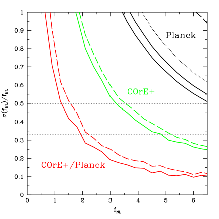
Figure 6: The relative uncertainty for positive $f_{\text{NL}}$ obtained by Fisher forecasts for Planck (black lines), COrE+ (green lines) and a combination of COrE+ and Planck (red lines). The two black solid lines are for Planck with $f_{\text{sky}}=0.2$ (upper) and 0.4 (lower curve; the case with $f_{\text{sky}}=0.6$ is very close to the case with 0.4); the dotted black line is for $f_{\text{sky}}=0.1$ and the dashed line (in the upper–right corner) for $f_{\text{sky}}=0.8$. For COrE+, the solid (dashed) green line corresponds to the configuration with 4 (3) CIB frequency maps. The red dashed line is for COrE+ adding only the 857–GHz channels, and the solid line adding all the Planck frequencies $\geq 353$ GHz (see the text and Table 4)

Figure 7: The value of $f_{\text{NL}}$ for which its relative uncertainty is equal to 1 (solid lines, corresponding to a $1\sigma$ detection), 1/2 (long dased lines) and 1/3 (short dashed lines) is plotted as a function of the fraction of the dust residual. This is computed for Planck (left panel), COrE+ (middle panel) and the combination COrE+/Planck (right panel), in their best configuration for CIB measurements.

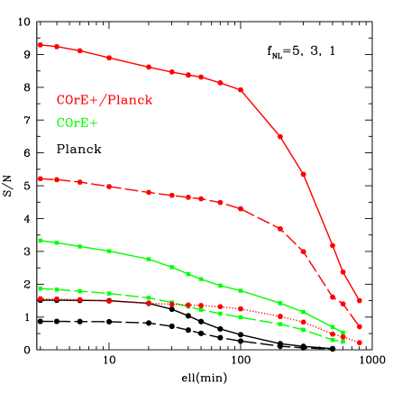
Figure 8: Signal–to–noise ratio for $f_{\text{NL}}=5,$ 3 and 1 (solid, dashed and dotted lines, respectively) as expected for Planck (red lines), COrE+ (green lines) and the combination COrE+/Planck (red lines). This is computed for $f_{\text{sky}}=0.4$ and 1% dust residual.

4.3 Fisher forecasts for present and future experiments

In this section we aim to provide realistic forecasts for the detection of the $f_{\text{NL}}$ parameter including 1) the Galactic dust contamination, as discussed above, and 2) the instrumental properties of CMB space missions. We focus on Planck, and on possible future experiments like COrE+, LiteBIRD (Matsumura et al., 2014) and PIXIE (Kogut et al., 2014). Table 4 gives the instrumental specifications we consider for these experiments. We take into account frequencies $\nu>200$ GHz solely.

Planck. Observations from the Planck mission cover a large range of frequencies, up to 857 GHz. The 545– and 857–GHz channels are crucial for the CIB/dust separation. In our analysis we suppose that the channels at 353 and 857 GHz are dedicated to provide the dust template, while CIB maps are recovered at 217 and 545 GHz. In Table 4 we report the degraded sensitivity in these channels after the subtraction of the dust contamination (see Eq. 39). In this particular case, the 217–GHz channel gains, in term of (squared) sensitivity, a factor $\sim 1.5$, while the 545–GHz channel loses sensitivity by almost a factor 6.

Assuming that the dust emission has been cleaned at a level of 1%, we find that the uncertainty on $f_{\text{NL}}$ provided by Planck is $\sigma(f_{\text{NL}})\simeq 3.5$, almost independently of the value of $f_{\text{NL}}$. In Figure 6 we show the relative uncertainty on $f_{\text{NL}}$. According to our estimates, Planck should be able to detect $|f_{\text{NL}}|$ at about 2–$\sigma$ level if it is larger than 6, and give an upper limit of $\sim 3.5$ at 1–$\sigma$. This would significantly improve the current constraints on the local $f_{\text{NL}}$ provided by Planck using the CMB bispectrum (Planck Collaboration XVII, 2015), i.e. $f_{\text{NL}}=0.8\pm 5.0$.

We have also considered CIB maps covering different fractions of the sky. The optimal configurations have a sky fraction $f_{\text{sky}}\simeq 0.4$, although similar results are obtained for $0.2~{}\hbox to0.0pt{$<$\hss}{\lower 4.30554pt\hbox{$\sim$}}f_{\text{sky}}~{}\hbox to0.0pt{$<$\hss}{\lower 4.30554pt\hbox{$\sim$}}0.6$. For smaller areas, the sensitivity to $f_{\text{NL}}$ gets worse, while very large fractions of the sky are not useful for the $f_{\text{NL}}$ detection due to the strong dust contamination. Finally, we show in Figure 7 the dependence of our results on the amplitude of the dust residual. The possible detection of $f_{\text{NL}}$ strongly depends on the dust contamination. In order to improve the current Planck constraint on $f_{\text{NL}}$, dust contamination has to be removed at least at a 3% level. On the other hand, a 1 per mil cleaning would give an uncertainty of $\sigma(f_{\text{NL}})\simeq 2$.

COrE+. This project represents an approximately optimal space mission for the search of the CMB B–mode polarization, characterized by a high sensitivity of a few $\mu$K–arcmin, a few arcmin resolution and a large frequency coverage. The COrE+ project is planned to include 8 frequencies at $\nu>200$ GHz, with the highest channel at 600 GHz. We consider two possible configurations for the measurement of the CIB: a more conservative choice involving 3 frequencies for CIB and 5 for dust, and a optimistic one with half of the frequencies reserved for each component (see Table 4). In both cases, after the component separation, the noise in the reconstructed CIB maps increases by a factor 5–10. This significant degradation in sensitivity may be related to the frequency coverage, which does not include the wavelengths at which the SEDs of the two components start to differ. As expected however, the sensitivity on $f_{\text{NL}}$ significantly increases with respect to Planck, being $\sigma(f_{\text{NL}})\ga 1.6$. Consequently, $|f_{\text{NL}}|=5$ would be measured at $\sim 3$–$\sigma$, and $|f_{\text{NL}}|$ of 2–3 would be also detectable with a significance of about 1– 2 $\sigma$ (see Figure 6). The difference between the two configurations is modest, although an extra CIB frequency has been added. Here again, the best results are for sky fractions around 0.4–0.6. Looking at Figure 7, the COrE+ results appear to be less dependent on the dust residual, presumably owing to the higher instrumental sensitivity.

COrE+/Planck. The sensitivity of COrE+ to the $f_{\text{NL}}$ parameter strongly improves when the highest Planck channels are also taken into account and combined with COrE+ data. Extending the frequency coverage to 857 GHz is key to better separate CIB and dust emission. It is actually enough to include the Planck 857–GHz channel in the mixing matrix to reduce the noise degradation in reconstructed CIB maps, at a level close to the COrE+ sensitivity (see Table 4). This is due to the different scaling of the dust and the CIB at high frequencies, see Fig. 5. In Figure 6 we show the results when Planck data are included to estimate the mixing matrix and the noise degradation. We see that a 3– (2–)$\sigma$ detection of $|f_{\text{NL}}|$ is now possible down to values of 2 (1.5). This means that, with this configuration, the residual dust emission can be accurately separated from the CIB fluctuations. This is confirmed by the fact that reducing the level of the dust residual there is a very small improvement in the detection of $f_{\text{NL}}$ (see Figure 7). In addition, if we increase the fraction of the sky up to $f_{\text{sky}}=0.8$, $\sigma(f_{\text{NL}})$ always decreases.

Figure 8 shows the signal–to–noise ratio (defined as ${\rm SNR}=f_{\text{NL}}/\sigma(f_{\text{NL}})$) for $f_{\text{NL}}$ as a function of the minimum observable multipole $\ell_{\text{min}}$ for the three cases discussed above. It is interesting to note that for Planck the SNR is constant up to $\ell_{\text{min}}=20$, indicating that at the largest angular scales the signal is completely dominated by the dust contamination. On the contrary, COrE+ succeeds to better separate the two components and to access information also at $\ell~{}\hbox to0.0pt{$<$\hss}{\lower 4.30554pt\hbox{$\sim$}}20$. The multipole range that contributes the most to the SNR changes according to the experiment and the configuration: in Planck this range is about $\ell=20$–70; in COrE+ it extends almost up to $\ell=300$–400; in COrE+/Planck large angular scales seem to contribute less than in the previous examples, and the SNR clearly drops only at $\ell>100$ and the main contribution comes from scales between $\ell\sim 100$ and $~{}\hbox to0.0pt{$<$\hss}{\lower 4.30554pt\hbox{$\sim$}}600$.

LiteBIRD. This satellite could provide interesting constraints on $f_{\text{NL}}$ in its extended version, with several spectral bands spanning 40–400 GHz and 4 bands between 200 and 400 GHz. Clearly, without external information, LiteBIRD alone is not suitable for detecting PNG through the CIB ($\sigma(f_{\text{NL}})\ga 6$, see Table 4). However, jointly with Planck data, we find $\sigma(f_{\text{NL}})\simeq 1.3$ (in a configuration where three out of four LiteBIRD channels are dedicated to the CIB), only a factor 2 larger than with COrE+.

PIXIE. The planned PIXIE mission presents almost the optimal requirements for detecting $f_{\text{NL}}$ through CIB anisotropies, thanks to its 400 channels between 30 GHz and 6 THz and a rms sensitivity of the order of 70 nK in $1^{\circ}$ pixels. In these conditions, dust emission should be extremely well constrained, even at the peak of the thermal emission. We expect therefore that PIXIE will be able to investigate very tiny PNG signals, with $|f_{\text{NL}}|\ll 1$. As an example, we have considered 8 frequency bands between 200 and 600 GHz with a squared sensitivity of 1 Jy sr^-1 and a resolution of $1.6^{\circ}$: we obtain $\sigma(f_{\text{NL}})\simeq 0.08$ assuming 1% of dust residual and $\sim 0.07$ without dust contamination. Extending the frequency range to 900 GHz (but with a similar number of frequency bands) seems not to produce any relevant improvement in the $f_{\text{NL}}$ uncertainty. However, these results should be taken as indicative. On one hand, we expect that increasing the number of frequency bands dedicated to CIB, $\sigma(f_{\text{NL}})$ could still decrease. On the other hand, especially for the PIXIE case that can investigate very low values of $f_{\text{NL}}$, a more accurate analysis should be required, taking into account effects of other contaminants (CMB, extragalactic sources, etc.) and model uncertainties (e.g., in the CIB and bias prescriptions). We will discuss these issues in the next Section.

Table 4: Instrumental specifications of the space missions considered in the paper, the corresponding noise variance in the reconstructed CIB maps for different configurations ($\Sigma^{2}$) and the uncertainty on $f_{\text{NL}}$ (assuming $f_{\text{NL}}=0$).

	Planck											$\sigma(f_{\text{NL}})$
$\nu$ [GHz]		217			353			545		857
fwhm [arcmin]		5.02			4.94			4.83		4.64
w-1 [Jy2 sr${-1}$]		43.32			164.7			185.3		157.9
$\Sigma^{2}$ [Jy2 sr${-1}$]		29.0			–			1100		–		3.6
	COrE+
$\nu$ [GHz]		220	255	295	340	390	450	520	600
fwhm [arcmin]		3.82	3.29	2.85	2.47	2.15	1.87	1.62	1.40
w-1 [Jy2 sr${-1}$]		0.654	1.43	5.20	8.31	13.50	22.98	39.88	69.26
$\Sigma^{2}$ [Jy2 sr${-1}$]		–	8.03	–	47.3	–	–	377.	–			1.8
		–	8.04	–	47.3	–	212.	382.	–			1.6
with Planck 857 GHz		–	1.83	–	10.0	–	–	82.6	147.			0.7
with Planck		–	1.97	–	10.8	–	45.6	90.2	163.6			0.6
	LiteBIRD
$\nu$ [GHz]		235		280	337	402
fwhm [arcmin]		30		30	30	30
w-1 [Jy2 sr${-1}$]		0.36		1.45	1.1	0.7
$\Sigma^{2}$ [Jy2 sr${-1}$]		11.3			149.5							6.4
with Planck		1.0			6.7	14.6						1.3
	PIXIE
$\nu$ [GHz]		218	248	293	353	398	443	548	593
fwhm [arcmin]		96	96	96	96	96	96	96	96
$\Sigma^{2}$ [Jy2 sr${-1}$]		1.0	1.0	1.0	1.0	1.0	1.0	1.0	1.0			0.08
no dust		1.0	1.0	1.0	1.0	1.0	1.0	1.0	1.0			0.07

5 Discussion

Model of CIB power spectra. Our Fisher forecasts rely on the fact that the CIB model we adopt provides a good description of actual CIB spectra, at least on the angular scales of interest. This is a reasonable hypothesis, considering that the model is able to fit observations for auto– and cross–frequency power spectra, number counts, and absolute CIB levels simultaneously (Viero et al., 2013; Planck Collaboration XXX, 2014). However, although it successfully describes Planck data, it remains nonetheless a fairly simplified description of the actual CIB. Future high–quality CIB measurements (necessary to detect the $f_{\text{NL}}$ parameter) may require an additional level of sophistication.

The CIB angular power spectra are currently well determined only at small/intermediate angular scales, i.e. $\ell\ga 200$. No information is thus far available at larger scales, where the PNG effects on CIB anisotropies are most pronounced. Some concern could arise if the shape of the low–$\ell$ part of CIB spectra depends depends on model assumptions. To test this, we have compared the large–scale power spectra obtained with different CIB models, all providing a good fit to the Planck data. Besides the extended halo model used in this paper, we have considered: 1) a linear model where the 2–halo contribution is determined by an effective bias and by the star formation history, which in turn are constrained by Planck data (see §5.4 of Planck Collaboration XXX, 2014); 2) a simplified halo model in which all galaxies have the same luminosity regardless of their host dark matter halo used, e.g.. in Planck Collaboration XVIII (2011); Curto et al. (2015). Although they agree at $\ell\ga 200$, the power spectra exhibit a different behavior at the largest scales (see left panel of Figure 9). Our reference model peaks at higher angular scales and has significantly less power at $\ell~{}\hbox to0.0pt{$<$\hss}{\lower 4.30554pt\hbox{$\sim$}}100$. The main factor that determines the low–$\ell$ behavior in the CIB spectra is the redshift evolution of the average galaxy emissivity, $\bar{\jmath}_{\nu}(z)$. In fact, when the same $\bar{\jmath}_{\nu}(z)$ is applied to the different CIB models, the low–$\ell$ power spectra become very similar, and even indistinguishable (after a proper renormalization) as shown in the right panel of Figure 9. Overall, the PNG features in the CIB power spectra seem to weakly depend on the model prescription.

In order to distinguish PNG signals, it is therefore key to correctly model the evolution of the infrared galaxy emissivity. Accurate measurements of CIB power spectra at degree scales should further strengthen the model reliability, especially concerning this point. Estimates of number counts, luminosity and correlation functions of infrared galaxies at shorter wavelengths should also provide complementary information. In addition, as shown in Planck Collaboration XXX (2016), the evolution of the galaxy emissivity can be related to the star formation density history. The linear model and the extended halo model recover consistent star formation histories below $z=2$, in agreement with recent measurements by Spitzer and Herschel, while at higher redshifts, there are discrepancies between the two models and between models and observational estimates (see discussion in Planck Collaboration XXX, 2016). In the future, we expect that a better determination of the history of the star formation density will improve significantly the constraints on the galaxy emissivity and then will help to fix the CIB spectral behavior at low $\ell$s.

Moreover, we have shown in §2.3 that the relative amplitude of the non–Gaussian CIB bias could depend on the HOD parameter $M_{\text{eff}}$, i.e. on the range of halo masses that are most efficient at hosting star formation. In the extended halo model this parameter is assumed to be constant in time, in agreement with results from Behroozi et al. (2013), at least out to $z=4$. However, they found a much lower value for the characteristic halo mass (i.e. $\log(M_{\text{eff}}/M_{\odot})=11.7$) compared to the Planck results. We have verified that, using this value for $M_{\text{eff}}$, CIB spectra change in amplitude but not in shape, even with $f_{\text{NL}}\neq 0$. This is an important indication that the PNG signal is fairly insensitive to the HOD parameters. Note, however, that we have extrapolated the subhalo mass function of Tinker & Wetzel (2010) much beyond its actual range of validity, i.e. $0.8<z<1.6$. Furthermore, while the amplitude non-Gaussian bias is generally given by derivative of $\bar{n}_{h}$ relative to the normalisation $\sigma_{8}$ (Slosar et al., 2008), we have assumed a universal halo mass function $\bar{n}_{h}$, which implies $\partial{\rm ln}\bar{n}_{h}/\partial{\rm ln}\sigma_{8}=\delta_{c}b_{1}$. The validity of this assumption may, however, depend on the halo identification algorithm (Desjacques & Seljak, 2010). Although N-body simulations support universality when the mass of SO halos is $M\gtrsim 10^{13}M_{\odot}$ (Desjacques et al., 2009), the extent to which this assumption holds at smaller masses is still a matter of debate.

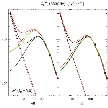
Figure 9: Left panel CIB power spectra with $f_{\text{NL}}=0$ and 5, according to different model approaches: the extended halo model used in the paper (solid black lines); the simplified halo model (red long dashed lines); the linear model (green dash–dotted line, only $f_{\text{NL}}=0$). Short dotted lines shows the difference between the Gaussian case and $f_{\text{NL}}=5$. Points represent Planck measurements (Planck Collaboration XXX, 2016). CIB spectra differ at $\ell<200$. Right panel The same as in the left panel, but here spectra are computed using the same galaxy emissivity evolution as given by the extended halo model. Differences in CIB spectra are now small or negligible over all the multipole range considered. In either case, the PNG signal seems to be independent on the model approach.

Galactic dust emission. Due to its relevance, we should investigate the extent to which our results are sensitive to the Galactic dust model used in the analysis. Dust residual in CIB reconstructed maps is parametrized – see Section 4.1 and Eq. (36) – by the product of spatial, frequency and correlation terms. In particular, by taking the correlation matrix $R_{\nu\nu^{\prime}}$ independent of the angular scale, we are supposing that the shape of dust residual power spectra are the same over all the frequencies. This is something expected and supported by simulations of component separation performance (Curto et al., 2016).

Two free parameters are considered for dust residual power spectra and then marginalized in the Fisher approach: the amplitude and the power–law index of the power spectrum at the reference frequency. The dust SED is instead assumed to be perfectly known. This is motivated by the fact that this Galactic contaminant largely dominates the sky emission at $\nu\ga 300$ GHz, especially on large angular scales, and the frequency spectrum is expected to be accurately determined across the sky. This hypothesis can be relaxed by adding as extra free parameter the dust emissivity index $\beta_{d}$. We have verified however that it has a negligible impact on the $f_{\text{NL}}$ uncertainty.

A more critical issue in the Fisher analysis is the frequency coherence in the dust residual. We have related it to the spatial dispersion of the dust emissivity index, according to the prescription proposed by Tegmark (1998). Planck Collaboration XXII (2015) found that the variance across the sky of the dust spectral index is $\Delta\beta\simeq 0.07$ which corresponds to a frequency correlation level larger than 99% (between 200 and 900 GHz). It is clear that reducing the frequency coherence of the dust emission can significantly degrade the sensitivity on the $f_{\text{NL}}$ parameter for experiments covering a large frequency range. In Table 5 we compute the frequency coherence values as increasing $\Delta\beta$. We can see that dust emission is still highly correlated for $\Delta\beta\simeq 0.1$, even between well separated frequencies, while some decorrelation is observed for $\Delta\beta\sim 0.3$ and $\nu/\nu^{\prime}>2$. The uncertainty on $f_{\text{NL}}$ from Planck or COrE+ seems to be quite sensitive to the frequency coherence and increases by $\sim 20$% if $\Delta\beta=0.1$. On the contrary, when Planck and COrE+ are combined, the frequency decorrelation has little impact on results.

Table 5: Frequency coherence of the dust emission and the uncertainty on the $f_{\text{NL}}$ parameters as a function of the spatial dispersion of the dust spectral index.

$\Delta\beta$	0.07	0.1	0.3	0.5
$\nu/\nu^{\prime}$	$R_{\nu\nu^{\prime}}$
1.5	$>0.99$	$>0.99$	0.985	0.96
2	$>0.99$	$>0.99$	0.96	0.89
3	$>0.99$	0.99	0.90	0.74
4	0.99	0.98	0.84	0.62
	$\sigma(f_{\text{NL}})$
Planck	3.6	4.2	7.5	9.1
COrE+	1.6	1.9	2.9	3.3
COrE+/Planck	0.6	0.64	0.72	0.76

Dust contamination and Fisher forecasts. As an alternative approach to estimate $f_{\text{NL}}$ constraints in the presence of dust contamination, we compute the Fisher matrix without assuming any foreground removal. We include in the analysis all the observational frequencies for a given experiment at their nominal sensitivity. We expect this approach to produce more conservative results. Dust removal on maps should be in fact more powerful and effective than a CIB–dust emission separation at the level of power spectra. It is also an useful test to check if our working hypothesis (e.g., dust removal at a 1 per cent level in about half of the observational frequencies) are too conservative or too optimistic. For Planck we find $\sigma(f_{\text{NL}})\simeq 5$, about a 50 per cent larger than previous results with 1% dust residual. In this case, a component separation approach to remove the dust contamination is strictly required. On the other hand, in the case of COrE+, if we consider all the 8 frequencies between 200 and 600 GHz at their nominal sensitivity, the uncertainty on $f_{\text{NL}}$ significantly decreases with respect to previous values, and we find $\sigma(f_{\text{NL}})\simeq 0.25$ (to be compared with $\sim 1.6$ and 0.6 for COrE+ and COrE+/Planck, respectively). This result is very close to the one obtained without any dust contamination in §3. Similarly, for LiteBIRD we obtain $\sigma(f_{\text{NL}})\simeq 0.33$. Such an improvement can be explained by the very small noise level expected in future experiments (not degraded by component separation) together with a larger number of frequency channels. We therefore conclude that, in principle, the dust contamination should be fully controlled by high–sensitive observations at a sufficient number of frequencies. Previous results for COrE+ and LiteBIRD mission might be then conservative, at least in terms of the number of frequencies to be exploited for the CIB.

For the purpose of computing the Fisher matrix we fixed the fiducial cosmological model. This assumption contributes to a possible theoretical systematic uncertainty. However, the Planck satellite has measured the parameters of the cosmological standard model to high precision (Planck Collaboration XIII, 2015). For example, the tilt of the primordial spectrum might be partially degenerate with the CIB slope at low $\ell$. But Planck has determined the value of the scalar spectral index with tiny error bars, $n_{s}=0.968\pm 0.006$. In addition, the Planck data covers a wide range of scales, and there is no indication for a running of the scalar spectral index or any other significant deviation from a power law spectrum, except maybe a (not significant) power deficit on large scales (Planck Collaboration XX, 2015). The power deficit can hardly be confused with the expected excess power on the largest scales in the CIB from non-Gaussian bias if $f_{\text{NL}}>0$, and also the curves for $f_{\text{NL}}<0$ turn back up at the lowest $\ell$ so that we do not expect this to be a problem.

Finally, we did not fully take into account the non-Gaussianity of the CIB covariance matrix, although the CIB power spectrum includes the non-Gaussian bias. We have ignored the contribution induced by a primordial four-point function (or trispectrum) which, in the PNG model considered here, is proportional to $f_{\text{NL}}^{2}$. This term might not be negligible at low multipoles. The covariance will also include contributions generated by the nonlinear gravitational evolution. They will involve, among others, the CIB bispectrum. However, these terms scale at best like $k^{2}$ in the power of biased tracers. Therefore, we expect them to contribute much less than the 1-halo term at low multipoles.

Overall, $\sigma(f_{\text{NL}})<1$ results should be taken with some caution. For example, according to our estimates, PIXIE has the potentiality to detect PNG signals from $f_{\text{NL}}<0.1$. However, as discussed in this section, our Fisher forecasts are based on some theoretical assumptions (e.g., the bias prescription, Gaussian covariance matrix, etc.), and on a particular CIB modeling framework, whose validity and impact on results has not been fully investigated. Finally, possible systematics in future data and extra astrophysical contaminants (as CMB, point sources, thermal Sunyaev–Zeldovich effect) have not been considered in the present analysis. All these aspects should be investigated in future works.

6 Conclusion

In this paper we investigate the ability of CIB observations at frequencies of a few hundred GHz (i.e. where CMB experiments operate) to detect local primordial non-Gaussianity, and measure the nonlinear parameter $f_{\text{NL}}$ by leveraging the scale dependent bias on large scales.

We model the CIB angular power spectrum under the assumption that the cosmic infrared background is produced by star–forming galaxies emitting at infrared wavelengths. We describe the clustering of these galaxies using a halo model, with a galaxy luminosity–halo mass relation as adopted in Shang et al. (2012); Planck Collaboration XXX (2014). We take into account both general relativistic corrections and the scale–dependent non–Gaussian halo bias induced by the local primordial non-Gaussianity. We perform a Fisher forecast to ascertain the precision at which $f_{\text{NL}}$ can be measured by CMB space missions.

We find that the GR corrections are subdominant except at the largest angular scales. The leading contribution arises from the Doppler term, although it only makes up less than 50% of the CIB angular power spectrum at 353 GHz for $\ell=2$ (where cosmic variance is largest), higher frequencies. At $\ell=10$, the GR corrections are reduced to the percent level, corresponding to a local bispectrum shape with amplitude $f_{\text{NL}}\simeq 0.1$.

Under the ideal condition of perfect dust subtraction over 40% of the sky, future CMB space missions like COrE+, operating at frequencies between 200 and 600 GHz, shall be able to detect $f_{\text{NL}}\sim 1$ with high significance ($>2\,\sigma$), when several frequencies are combined. In this case, information from the very large angular scales, i.e. the ones most affected by Galactic dust, is not strictly required.

Of course, a complete subtraction of dust is unlikely. Therefore, we have also produced forecasts assuming a dust subtraction at the 1% level in the best scenario. In this case, an experiment with a Planck–like sensitivity should be able to reach an uncertainty on $f_{\text{NL}}$ of $\sigma(f_{\text{NL}})\sim 3.5$ for sky fractions between 0.2 and 0.6. Larger sky fractions are not useful because of the strong dust contamination, which actually degrades the constraints. Future probes like COrE+, LiteBIRD and PIXIE, which have a higher sensitivity and more frequency channels, should be able to constrain $f_{\text{NL}}$ to much lower values, even in a situation where the lowest multipoles could not be used owing to foreground contamination, systematic effects, or a residual dust fraction higher than expected after the cleaning. We have found that the presence of high-frequency channels in the range of 800 to 1000 GHz is especially important to reduce the impact of dust and reach $|f_{\text{NL}}|<1$. Future missions should thus either include detectors at those frequencies or,alternatively, combine their data with the Planck 857 GHz to achieve this precision.

To conclude, an analysis of current CIB observations should in principle already yield bounds on the local $f_{\text{NL}}$ competitive with those obtained from the analysis of non-Gaussianity in the Planck CMB maps. The CIB holds the promise of reaching $|f_{\text{NL}}|~{}\hbox to0.0pt{$<$\hss}{\lower 4.30554pt\hbox{$\sim$}}1$ in a not so distant future. Although not considered here, additional information could also be harvested from a cross-correlation of the “CMB lensing potential” and CIB anisotropies. This is expected to be less sensitive to the PNG but, at the same time, less affected by dust contamination (Anthony Challinor, private communication). While direct observations of the large scale structure might eventually prove even more sensitive, the CIB will remain an invaluable tool to cross-check detections or limits from LSS due to the different systematics present in these various probes.

Appendix A General Relativistic corrections to the CIB intensity

We provide details about the calculation of the GR correction to the CIB brightness. We refer the reader to the intensity mapping studies of Hall et al. (2013); Alonso et al. (2015) for complementary information.

A.1 CIB brightness

Let $I(\nu_{o})$ be the observed CIB brightness (in units of Jy sr^-1), i.e. the amount of energy ${\rm d}E_{o}$ that passes through a proper surface element ${\rm d}A_{o}$ (transverse to the observed ray direction) per frequency interval ${\rm d}\nu_{o}$, per proper time ${\rm d}\tau_{o}$ and per solid angle $d\Omega_{o}$,

$$I(\nu_{o})=\frac{{\rm d}E_{o}}{{\rm d}\tau_{o}{\rm d}\nu_{o}{\rm d}\Omega_{o}{\rm d}A_{o}}\;.$$ (42)

The corresponding number of photons received by the observer is ${\rm d}N_{o}={\rm d}E_{o}/h\nu_{o}$. Conservation of photon number (which follows from Liouville’s phase space conservation law) implies ${\rm d}N_{o}={\rm d}N_{s}$, where $\d{d}N_{s}$ is the infinitesimal number of photons emitted by the source. Namely,

$$I(\nu_{o}) =\frac{\nu_{o}}{\nu_{s}}\frac{{\rm d}E_{s}}{{\rm d}\tau_{s}{\rm d}\nu_{s}{\rm d}\Omega_{s}{\rm d}A_{s}}\,\frac{{\rm d}\tau_{s}{\rm d}\nu_{s}}{{\rm d}\tau_{o}{\rm d}\nu_{o}}\,\frac{{\rm d}\Omega_{s}{\rm d}A_{s}}{{\rm d}\Omega_{o}{\rm d}A_{o}}$$ (43)

$$=\left(1+z\right)^{-3}\frac{{\rm d}E_{s}}{{\rm d}\tau_{s}{\rm d}\nu_{s}{\rm d}\Omega_{s}{\rm d}A_{s}}\;.$$

To derive the second equality, we have used $\nu_{o}/\nu_{s}={\rm d}\tau_{s}/{\rm d}\tau_{o}=(1+z)^{-1}$ and the reciprocity relation $D_{L}=(1+z)D_{A}$, where $D_{A}=\sqrt{{\rm d}A_{s}/{\rm d}\Omega_{o}}$ and $D_{L}=\sqrt{{\rm d}A_{o}/{\rm d}\Omega_{s}}$ are the angular diameter distance and (redshift-corrected) luminosity distance, respectively. Note that the luminosity and angular distances have canceled each other out of the last expression.

Let $\lambda$ be the affine parameter of the light ray $x^{\mu}(\lambda)$, so that $k^{\mu}={\rm d}x^{\mu}/{\rm d}\lambda$ is its wavevector. During an interval $d\lambda$, the wavefront seeps out a proper volume ${\rm d}V_{s}={\rm d}l_{s}{\rm d}A_{s}$, where ${\rm d}l_{s}=k_{\mu}u^{\mu}_{s}{\rm d}\lambda$ is proportional to the 4-velocity $u_{s}^{\mu}$ of the emitter. Therefore, the above relation becomes

$$I(\nu_{o}) =\left(1+z\right)^{-3}\,\frac{{\rm d}E_{s}}{{\rm d}\tau_{s}{\rm d}\nu_{s}{\rm d}\Omega_{s}{\rm d}V_{s}}\,(k_{\mu}u^{\mu}_{s}){\rm d}\lambda$$ (44)

$$=\left(1+z\right)^{-3}\jmath_{\nu_{s}}^{\text{\tiny phys}}\,(k_{\mu}u_{s}^{\mu}){\rm d}\lambda\;,$$

where

$$\jmath_{\nu_{s}}^{\text{\tiny phys}}=\frac{{\rm d}E_{s}}{{\rm d}\tau_{s}{\rm d}\nu_{s}{\rm d}\Omega_{s}{\rm d}V_{s}}$$ (45)

is the source emissivity per physical volume (in unit of Jy sr^-1 m^-1). In the case of a continuous medium, Eq. (44) must be integrated along the light ray. Hence, we can write

$$I(\nu_{o},\mathrm{\hat{\textbf{\em n}}})=\int\!\!{\rm d}\lambda\,(k_{\mu}u_{s}^{\mu})\,\frac{\jmath_{(1+z)\nu_{o}}^{\text{\tiny phys}}\!(\lambda)}{(1+z)^{3}}\;,$$ (46)

where $\mathrm{\hat{\textbf{\em n}}}$ is the observed angular position. In principle, we should also take into account the loss of intensity as the photons propagate through the intergalactic medium and modify the above relation accordingly:

$$I(\nu_{o},\mathrm{\hat{\textbf{\em n}}})=\int\!\!{\rm d}\lambda\,(k_{\mu}u_{s}^{\mu})\,\frac{\jmath_{(1+z)\nu_{o}}^{\text{\tiny phys}}\!(\lambda)}{(1+z)^{3}}e^{-\tau(\nu_{o},\mathrm{\hat{\textbf{\em n}}},\lambda)}\;,$$ (47)

where $\tau(\nu_{o},\mathrm{\hat{\textbf{\em n}}},\lambda)$ is the optical depth along the path of the ray. For simplicity however, we will ignore the beam absorption in what follows, as the focus is the evaluation of Eq. (46) at linear order in metric perturbations.

A.2 GR corrections at first order in perturbations

We consider a perturbed FRW metric in the conformal Newtonian gauge with coordinates $x^{\mu}=(\eta,x^{i})$,

$${\rm d}s^{2}=a^{2}(\eta)\big{(}\eta_{\mu\nu}+h_{\mu\nu}\big{)}{\rm d}x^{\mu}{\rm d}x^{\nu}\;,$$ (48)

where

$$h_{00}=-2\Psi\;,\qquad h_{0i}=0\;,\qquad h_{ij}=-2\Phi\delta_{ij}\;.$$ (49)

The perturbed photon wavevector $k^{\mu}={\rm d}x^{\mu}/{\rm d}\lambda$ corresponding to the light ray $x^{\mu}(\lambda)$ can be written as

$$k^{\mu}=\frac{1}{a^{2}}\big{(}-1+\delta\nu,\mathrm{\hat{\textbf{\em n}}}+\delta\mathrm{\hat{\textbf{\em n}}}\big{)}\;,$$ (50)

where $\delta\nu$ is the fractional frequency perturbation and $\delta\mathrm{\hat{\textbf{\em n}}}$ is the change in the propagation direction, which is such that $\mathrm{\hat{\textbf{\em n}}}^{2}=1$ and $\mathrm{\hat{\textbf{\em n}}}\cdot\delta\mathrm{\hat{\textbf{\em n}}}=0$. Since lightlike geodesics are conformally invariant, the metric $(\eta_{\mu\nu}+h_{\mu\nu}){\rm d}x^{\mu}{\rm d}x^{\nu}$ admits the same photon geodesics which we parametrize as $x^{\mu}(\tilde{\lambda})$. The corresponding photon wavevector $\tilde{k}^{\mu}={\rm d}x^{\mu}/{\rm d}\tilde{\lambda}$ is related to $k^{\mu}$ through

$$\tilde{k}^{\mu}=a^{2}k^{\mu}\;.$$ (51)

Hence, the two affine parameters satisfy $\lambda=a^{2}\tilde{\lambda}$ up to an irrelevant constant.

We calculate the change in the perturbed photon wavevector $\tilde{k}^{\mu}$ using the geodesic equation

$$\frac{{\rm d}}{{\rm d}\tilde{\lambda}}\tilde{k}^{\mu}=-\Gamma^{\mu}_{\alpha\beta}\tilde{k}^{\alpha}\tilde{k}^{\beta}\;,$$ (52)

where $\Gamma^{\mu}_{\nu\lambda}$ are the Christoffel symbols in the conformally transformed metric. At linear order in perturbations, only the first geodesic equation describing the frequency shift is relevant as lensing of the uniform CIB yields the same CIB. Nonetheless, lensing magnification induces a first order perturbation to the CIB brightness through the flux limiting value. We will discuss this effect below. The relevant Christoffel symbols are $\Gamma^{0}_{00}=\dot{\Psi}$, $\Gamma^{0}_{0i}=\Psi_{,i}$ and $\Gamma^{0}_{ij}=-\dot{\Phi}\delta_{ij}$, where $\dot{X}$ and $X_{,i}$ designate a derivative w.r.t. $\eta$ and $x^{i}$, respectively. Linearizing the first geodesic equation, we arrive at

$$\frac{{\rm d}}{{\rm d}\tilde{\lambda}}\delta\nu=2\frac{{\rm d}\Psi}{{\rm d}\tilde{\lambda}}+\dot{\Psi}+\dot{\Phi}$$ (53)

upon taking advantage of the fact that the derivative w.r.t. $\tilde{\lambda}$ is

$$\frac{{\rm d}}{{\rm d}\tilde{\lambda}}\equiv\tilde{k}^{\mu}\partial_{\mu}\approx-\partial_{\eta}+\mathit{\hat{n}}^{i}\partial_{i}$$ (54)

at first order in perturbations. Eq. (53) easily integrates to

$$\delta\nu(\lambda)-\delta\nu_{o}=2\big{(}\Psi(\lambda)-\Psi_{o}\big{)}+\int_{0}^{\lambda}\!\!{\rm d}\lambda^{\prime}\big{(}\dot{\Psi}+\dot{\Phi}\big{)}\;.$$ (55)

It is now expressed in terms of the affine parameter $\lambda$, which we assume to be $\lambda=0$ at the observer position. Furthermore, $\Psi_{o}=\Psi(\lambda=0)$, $\delta\nu_{o}=\delta\nu(\lambda=0)$ etc.

Assuming that the source at affine parameter $\lambda$ (a galaxy contributing to the CIB) and the observer move with a 4-velocity $u^{\mu}=a^{-1}(1-\Psi,v^{i})$ and $u_{o}^{\mu}=a_{o}^{-1}(1-\Psi_{o},v_{o}^{i})$, where $v_{i}$ is the proper peculiar velocity, the redshift of the emitter relative to the observer (which could be measured if e.g. emission lines were resolved) is

$$1+z(\lambda)=\frac{\big{(}a^{-2}u_{\mu}\tilde{k}^{\mu}\big{)}_{\lambda}}{\big{(}a^{-2}u_{\mu}\tilde{k}^{\mu}\big{)}_{o}}\equiv\frac{1+\delta z(\lambda)}{a\big{(}\eta(\lambda)\big{)}}\;,$$ (56)

where $1/a\big{(}\eta(\lambda)\big{)}$ is the source redshift in an unperturbed universe, and

$$\delta z(\lambda)=-(\Psi-\Psi_{o})-\int_{0}^{\lambda}\!\!{\rm d}\lambda^{\prime}\,\big{(}\dot{\Psi}+\dot{\Phi}\big{)}+(\textbf{\em v}-\textbf{\em v}_{o})\cdot\mathrm{\hat{\textbf{\em n}}}$$ (57)

is the redshift perturbation. Note that the boundary terms at the observer position generate an unmeasurable monopole ($-\Psi_{o}$) and a dipole ($\textbf{\em v}_{o}\cdot\mathrm{\hat{\textbf{\em n}}}$), which we will ignore in what follows.

Since the emissivity $\jmath_{\nu}^{\text{\tiny phys}}$ explicitly depends on the observed redshift through $\nu=(1+z)\nu_{o}$, it is convenient to re-parametrize the light ray as a function of $z$, so that

$$I(\nu_{o};\mathrm{\hat{\textbf{\em n}}})=\int\!\!{\rm d}z\,\left(k_{\mu}u^{\mu}\frac{{\rm d}\lambda}{{\rm d}z}\right)\,\frac{\jmath_{(1+z)\nu_{o}}^{\text{\tiny phys}}\!\!(z,\textbf{\em x}(z))}{(1+z)^{3}}\;.$$ (58)

Therefore, fluctuations are now defined at the hypersurfaces of constant observed redshift $z$. We begin by evaluating the term $k_{\mu}u^{\mu}({\rm d}\lambda/{\rm d}z)$. Using $k_{\mu}u^{\mu}=a^{-1}(\eta)(1+z)$ with $z(\lambda)$ given by Eq. (56), we obtain

$$k_{\mu}u^{\mu}\frac{{\rm d}\lambda}{{\rm d}z}=\frac{a^{2}(\eta(z))}{{\cal H}(\eta(z))}\left(1+\delta\nu-\frac{a^{2}(\eta(z))}{{\cal H}(\eta(z))}\frac{{\rm d}\delta z}{{\rm d}\lambda}\right)\;.$$ (59)

We must now take into account the fact that the coordinate time fluctuates at fixed observed redshift $z$. Writing $\eta(z)=\bar{\eta}(z)+\delta\eta$, where $\bar{\eta}$ is the conformal time corresponding to the observed redshift $z$ in the unperturbed background, the perturbation to $a^{2}/{\cal H}$ reads

$$\frac{a^{2}(\eta)}{{\cal H}(\eta)}=\frac{a^{2}(z)}{{\cal H}(z)}\left[1+\left(2{\cal H}-\frac{\dot{\cal H}}{{\cal H}}\right)\delta\eta\right]\;,$$ (60)

where $a(z)\equiv a(\bar{\eta}(z))$, ${\cal H}(z)\equiv{\cal H}(\bar{\eta}(z))$ and the overdot designates a derivative w.r.t. $\bar{\eta}$. The time perturbation $\delta\eta$ can be read off from Eqs. (56) and (57) as

$${\cal H}\delta\eta=-\Psi-\int_{0}^{\lambda(z)}\!\!{\rm d}\lambda^{\prime}\big{(}\dot{\Psi}+\dot{\Phi}\big{)}+\textbf{\em v}\cdot\mathrm{\hat{\textbf{\em n}}}\;.$$ (61)

Here, $\lambda(z)$ is the value of the affine parameter at the observed redshift $z$. Therefore, with the help of the relation ${\cal H}\delta\eta+\delta\nu=\Psi+\textbf{\em v}\cdot\mathrm{\hat{\textbf{\em n}}}$, we eventually arrive at

$$k_{\mu}u^{\mu}\frac{{\rm d}\lambda}{{\rm d}z}=\frac{a^{2}(z)}{{\cal H}(z)}\left(1+\delta_{\parallel}\right)$$ (62)

where

$$\delta_{\parallel} =-\bigg{(}\frac{\dot{\cal H}}{\cal H}-{\cal H}\bigg{)}\delta\eta+\Psi+\textbf{\em v}\cdot\mathrm{\hat{\textbf{\em n}}}$$ (63)

$$\qquad+\frac{a^{2}(z)}{{\cal H}(z)}\bigg{[}\frac{{\rm d}\Psi}{{\rm d}\lambda}+\big{(}\dot{\Psi}+\dot{\Phi}\big{)}-\frac{{\rm d}\textbf{\em v}}{{\rm d}\lambda}\cdot\mathrm{\hat{\textbf{\em n}}}\bigg{]}$$

is the fractional change in ${\rm d}l_{s}$, i.e. in the source volume element along the line of sight. Note that the second term in the square brackets can be evaluated using $({\rm d}/{\rm d}\tilde{\lambda})=a^{2}({\rm d}/{\rm d}\lambda)$.

We now turn to the emissivity $\jmath^{\text{\tiny phys}}_{\nu}$. With the time slicing adopted here, perturbations to the emissivity are defined at constant observed redshift $z$:

$$a^{3}\jmath_{\nu}^{\text{\tiny phys}}(z,\textbf{\em x})=a^{3}(z)\,\bar{\jmath}_{\nu}^{\text{\tiny phys}}(z)\Big{(}1+\delta_{\jmath}^{z}(z,\textbf{\em x})\Big{)}\;,$$ (64)

where it is understood that all quantities are evaluated at a frequency $\nu=(1+z)\nu_{o}$. In practice, it is useful to relate the (gauge-invariant) fluctuation $\delta_{\jmath}^{z}$ to the perturbation $\delta_{\jmath}^{N}$ in the conformal Newtonian gauge adopted for this calculation. $\delta_{\jmath}^{N}$ is defined on slices of constant coordinate time $\eta$, whence

$$a^{3}(z)\bar{\jmath}_{\nu}^{\text{\tiny phys}}(z)\Big{(}1+\delta_{\jmath}^{z}(z,\textbf{\em x})\Big{)}=a^{3}(\eta)\bar{\jmath}_{\nu}^{\text{\tiny phys}}(\eta)\Big{(}1+\delta_{\jmath}^{N}(\eta,\textbf{\em x})\Big{)}$$ (65)

Since, at fixed observed redshift, $\eta(z)=\bar{\eta}(z)+\delta\eta$ where $\delta\eta$ is given by Eq. (61), we find after some algebra

$$\delta_{\jmath}^{z}=\delta_{\jmath}^{N}+\left(\frac{\dot{\bar{\jmath}}_{\nu}^{\text{\tiny phys}}}{\bar{\jmath}_{\nu}^{\text{\tiny phys}}}+3{\cal H}\right)\delta\eta=\delta_{\jmath}^{N}+\frac{\dot{\bar{\jmath}}_{\nu}}{\bar{\jmath}_{\nu}}\delta\eta$$ (66)

at first order in perturbations. Here and henceforth, $\jmath_{\nu}=a^{3}\jmath_{\nu}^{\text{\tiny phys}}$ is the comoving emissivity. Taking into account the factor $(1+z)^{-3}\equiv a^{3}(z)$ in Eq. (58), the CIB brightness simplifies to

$$I(\nu_{o};\mathrm{\hat{\textbf{\em n}}})=\int\!\!{\rm d}z\,\frac{a^{2}(z)}{{\cal H}(z)}\bar{\jmath}_{\nu}(z)\left(1+\delta_{\jmath}^{N}+\frac{\partial{\rm ln}\bar{\jmath}_{\nu}}{\partial\bar{\eta}}\delta\eta+\delta_{\parallel}\right)\;,$$ (67)

with $\nu=(1+z)\nu_{o}$.

Lastly, we must also take into account the fact that the CIB is produced by sources below a certain flux limiting value $S_{\nu}^{\text{\tiny cut}}$. Owing to fluctuations in the luminosity distance, this corresponds to a maximum luminosity $L_{\nu}^{\text{\tiny cut}}(z,\mathrm{\hat{\textbf{\em n}}})$ which depends on redshift and position on the sky. At first order in perturbations, we get

$$L_{\nu}^{\text{\tiny cut}}(z,\mathrm{\hat{\textbf{\em n}}})=\bar{L}_{\nu}^{\text{\tiny cut}}(z)\big{(}1+2\delta_{\perp}\big{)}\;.$$ (68)

The threshold luminosity $\bar{L}_{\text{\tiny cut}}(z)$ is related to the flux detection limit $S_{\text{\tiny cut}}$ through

$$\bar{L}_{\nu}^{\text{\tiny cut}}(z)=4\pi\big{(}1+z\big{)}^{4}a^{2}(z)\bar{\chi}^{2}(z)S_{\nu}^{\text{\tiny cut}}\;,$$ (69)

where $\bar{\chi}(z)$ is the line-of-sight comoving distance corresponding to the redshift $z$ in the unperturbed background. The perturbation $\delta_{\perp}$ transverse to the photon propagation at the source position is given by Eq. (19). Therefore, the average CIB emissivity $\bar{\jmath}_{\nu}$ per comoving volume in Eq. (67) should be replaced by

$$\int_{0}^{L_{\nu}^{\text{\tiny cut}}(z,\mathrm{\hat{\textbf{\em n}}})}\!\!\!{\rm d}L\,\bar{n}_{g}(L,z)\frac{L_{(1+z)\nu}}{4\pi}\\ =\bar{\jmath}_{\nu}(z)+2\,\bar{n}_{g}\big{(}\bar{L}_{\nu}^{\text{\tiny cut}}(z)\big{)}\frac{\bar{L}_{\nu}^{\text{\tiny cut}}(z)}{4\pi}\delta_{\perp}\;,$$ (70)

where, in $\bar{\jmath}_{\nu}(z)$, the integral over galaxy luminosities runs from 0 to $\bar{L}_{\nu}^{\text{\tiny cut}}(z)$. The perturbed CIB comoving emissivity at hypersurfaces of constant observed redshift thus reads

$$\jmath_{\nu}(z,\textbf{\em x})=\bar{\jmath}_{\nu}(z)\left(1+\delta_{\jmath}^{N}+\frac{\partial{\rm ln}\bar{\jmath}_{\nu}}{\partial\eta}\delta\eta+\delta_{\parallel}+2\frac{\bar{n}_{g}}{\bar{\jmath}_{\nu}}\frac{\bar{L}_{\nu}^{\text{\tiny cut}}}{4\pi}\delta_{\perp}\right)$$ (71)

for a given flux detection limit $S_{\nu}^{\text{\tiny cut}}$.

Finally, all the background quantities are thus far been evaluated at $\bar{\eta}(z)$. However, since the unperturbed photon path can also be parametrized as $x^{\mu}(\bar{\chi})=(\eta_{0}-\bar{\chi},\bar{\chi})$, we can recast the CIB brightness into Eq. (15) with the aid of ${\rm d}\bar{\chi}/{\rm d}z=a(\bar{\eta}(z))/{\cal H}(\bar{\eta}(z))$.

A.3 Imprint on the CIB angular power spectrum

Fluctuations in the CIB intensity can be expanded in the basis of spherical harmonics $Y_{\ell}^{m}$ as

$$I(\nu,\mathrm{\hat{\textbf{\em n}}})=\sum_{\ell m}a_{\ell m}(\nu)Y_{\ell}^{m}(\mathrm{\hat{\textbf{\em n}}})\;.$$ (72)

The frequency-dependent multipoles $a_{\ell m}(\nu)$ are given by the line-of-sight integral

$$a_{\ell m}(\nu)=\int\!\!{\rm d}z\left(\frac{{\rm d}\chi}{{\rm d}z}\right)\,a(z)\bar{\jmath}_{\nu}(z)\,\Delta_{\ell m}(\nu,z)\;,$$ (73)

where $\chi$ now is the unperturbed line-of-sight comoving distance (we drop hereafter the overline for shorthand convenience), and

$$\Delta_{\ell m}(\nu,z) =\int\!\!{\rm d}\mathrm{\hat{\textbf{\em n}}}\,Y_{\ell}^{m\star}\!(\mathrm{\hat{\textbf{\em n}}})\,\left(\delta_{\jmath}^{N}+\frac{\dot{\bar{\jmath}}_{\nu}}{\bar{\jmath}_{\nu}}\delta\eta+\delta_{\parallel}+2\frac{\bar{n}_{g}}{\bar{\jmath}_{\nu}}\frac{\bar{L}_{\text{\tiny cut}}}{4\pi}\delta_{\perp}\right)$$

$$=\sum_{S}\Delta_{\ell m}^{S}(\nu,z)$$ (74)

has been schematically decomposed in §2.2 into a sum of contributions induced by the first-order Newtonian gauge perturbations $\Psi$, $\Phi$, $v$ and the synchronous gauge density $\delta_{m}^{\text{\tiny syn}}$. Going to Fourier space and using the plane-wave expansion, some of the basic building blocks are, for instance,

$$\Delta_{\ell m}^{\Phi} =\frac{i^{\ell}}{2\pi^{2}}\int\!\!{\rm d}^{3}k\,T_{\Phi}(k,\chi)j_{\ell}(k\chi)Y_{\ell}^{m\star}\!(\mathrm{\hat{\textbf{\em k}}})\,\Phi_{i}(\textbf{\em k})$$ (75)

$$\Delta_{\ell m}^{\textbf{\em v}\cdot\mathrm{\hat{\textbf{\em n}}}} =\frac{i^{\ell}}{2\pi^{2}}\int\!\!{\rm d}^{3}k\,T_{v}(k,\chi)j_{\ell}^{\prime}(k\chi)Y_{\ell}^{m\star}\!(\mathrm{\hat{\textbf{\em k}}})\,\Phi_{i}(\textbf{\em k})$$

$$\Delta_{\ell m}^{\frac{{\rm d}\textbf{\em v}}{{\rm d}\eta}\cdot\mathrm{\hat{\textbf{\em n}}}} =-\frac{i^{\ell}}{2\pi^{2}}\int\!\!{\rm d}^{3}k\,k\,T_{v}(k,\chi)j_{\ell}^{\prime\prime}(k\chi)Y_{\ell}^{m\star}\!(\mathrm{\hat{\textbf{\em k}}})\,\Phi_{i}(\textbf{\em k})\;.$$

In the second line, the prime denotes a derivative w.r.t. the argument of the spherical bessel function $j_{\ell}(x)$. Total derivatives w.r.t. the unperturbed conformal time, ${\rm d}/{\rm d}\eta\equiv-{\rm d}/{\rm d}\chi$, bring an additional derivative w.r.t. the argument of $j_{\ell}(x)$.

Collecting all the terms and substituting into Eq. (73), we eventually arrive at

$$a_{\ell m}(\nu) =\frac{i^{\ell}}{2\pi^{2}}\int\!\!{\rm d}^{3}k\!\int\!\!{\rm d}z\left(\frac{{\rm d}\chi}{{\rm d}z}\right)\,a(z)\bar{\jmath}_{\nu}(z)$$ (76)

$$\qquad\times F_{\ell}(\nu,k,z)\,Y_{\ell}^{m\star}\!(\mathrm{\hat{\textbf{\em k}}})\Phi_{i}(\textbf{\em k})\;.$$

The radial window function $F_{\ell}(\nu,k,z)$ sourced by the perturbations $\delta_{\jmath}^{N}$, $\delta\eta$ and $\delta_{\parallel}$ is given by Eq. (27).

For the lensing magnification effect, which is not included in the Fisher analysis as it is small, $F_{\ell}(\nu,k,z)$ reads

$$F_{\ell}(\nu,k, z)=\bigg{\{}j_{\ell}(k\chi)\bigg{[}\left(\frac{1}{{\cal H}\chi}-1\right)T_{\Psi}-T_{\Phi}\bigg{]}+\left(\frac{1}{{\cal H}\chi}-1\right)$$

$$\qquad\times\int_{0}^{\chi}\!\!{\rm d}\chi^{\prime}\bigg{[}\big{(}T_{\Psi}+T_{\Phi}\big{)}+\frac{1}{\chi}\big{(}\dot{T}_{\Psi}+\dot{T}_{\Phi}\big{)}\bigg{]}j_{\ell}(k\chi^{\prime})$$

$$\quad+\frac{1}{2\chi}\int_{0}^{\chi}\!\!{\rm d}\chi^{\prime}\,\frac{\chi-\chi^{\prime}}{\chi^{\prime}}\big{(}T_{\Psi}+T_{\Phi}\big{)}j_{\ell}(k\chi^{\prime})$$

$$\quad+j_{\ell}^{\prime}(k\chi)\left(1-\frac{1}{{\cal H}\chi}\right)T_{v}\bigg{\}}2\,s(\chi)\;,$$ (77)

with the magnification bias $s(\chi)$ given by Eq. (16).

References

- Abell et al. (2009) Abell P. A., et al., 2009
- Agarwal et al. (2014) Agarwal N., Ho S., Shandera S., 2014, JCAP, 1402, 038
- Alonso et al. (2015) Alonso D., Bull P., Ferreira P. G., Maartens R., Santos M., 2015, Astrophys. J., 814, 145
- Alonso & Ferreira (2015) Alonso D., Ferreira P. G., 2015, Phys. Rev., D92, 063525
- Baldauf et al. (2011) Baldauf T., Seljak U., Senatore L., Zaldarriaga M., 2011, JCAP , 10, 031
- Bartolo et al. (2004) Bartolo N., Komatsu E., Matarrese S., Riotto A., 2004, Phys. Rept., 402, 103
- Behroozi et al. (2013) Behroozi P. S., Wechsler R. H., Conroy C., 2013, Astrophys. J. Lett., 762, L31
- Berlind & Weinberg (2002) Berlind A. A., Weinberg D. H., 2002, Astrophys. J., 575, 587
- Broadhurst et al. (1995) Broadhurst T. J., Taylor A. N., Peacock J. A., 1995, Astrophys. J., 438, 49
- Camera et al. (2015) Camera S., Maartens R., Santos M. G., 2015, Mon. Not. Roy. Astron. Soc., 451, L80
- Camera et al. (2015) Camera S., Santos M. G., Maartens R., 2015, Mon. Not. Roy. Astron. Soc., 448, 1035
- Carbone et al. (2010) Carbone C., Mena O., Verde L., 2010, JCAP, 1007, 020
- Challinor & Lewis (2011) Challinor A., Lewis A., 2011, Phys. Rev. D, 84, 043516
- Chen (2010) Chen X., 2010, Adv. Astron., 2010, 638979
- Cooray & Sheth (2002) Cooray A., Sheth R. K., 2002, Phys. Rept., 372, 1
- Curto et al. (2016) Curto A., Casaponsa B., et al. 2016, in preparation
- Curto et al. (2015) Curto A., Tucci M., Kunz M., Martinez-Gonzalez E., 2015, Mon. Not. Roy. Astron. Soc., 450, 3778
- Dalal et al. (2008) Dalal N., Dore O., Huterer D., Shirokov A., 2008, Phys. Rev., D77, 123514
- de Putter & Doré (2014) de Putter R., Doré O., 2014
- Desjacques et al. (2015) Desjacques V., Chluba J., Silk J., de Bernardis F., Doré O., 2015, Mon. Not. R. Astron. Soc., 451, 4460
- Desjacques & Seljak (2010) Desjacques V., Seljak U., 2010, Classical and Quantum Gravity, 27, 124011
- Desjacques et al. (2009) Desjacques V., Seljak U., Iliev I. T., 2009, Mon. Not. R. Astron. Soc., 396, 85
- Errard et al. (2016) Errard J., Feeney S. M., Peiris H. V., Jaffe A. H., 2016, JCAP , 3, 052
- Gangui et al. (1994) Gangui A., Lucchin F., Matarrese S., Mollerach S., 1994, Astrophys. J., 430, 447
- Giannantonio et al. (2014) Giannantonio T., Ross A. J., Percival W. J., Crittenden R., Bacher D., Kilbinger M., Nichol R., Weller J., 2014, Phys. Rev., D89, 023511
- Hall et al. (2013) Hall A., Bonvin C., Challinor A., 2013, Phys. Rev., D87, 064026
- Hall et al. (2010) Hall N. R., Keisler R., Knox L., Reichardt C. L., et al. 2010, Astrophys. J., 718, 632
- Hamaus et al. (2011) Hamaus N., Seljak U., Desjacques V., 2011, Phys. Rev., D84, 083509
- Jeong & Komatsu (2009) Jeong D., Komatsu E., 2009, Astrophys. J., 703, 1230
- Jeong et al. (2012) Jeong D., Schmidt F., Hirata C. M., 2012, Phys. Rev., D85, 023504
- Knox et al. (2001) Knox L., Cooray A., Eisenstein D., Haiman Z., 2001, Astrophys. J., 550, 7
- Kogut et al. (2014) Kogut A., Chuss D. T., Dotson J., Dwek E., Fixsen D. J., Halpern M., Hinshaw G. F., Meyer S., Moseley S. H., Seiffert M. D., Spergel D. N., Wollack E. J., 2014, in Space Telescopes and Instrumentation 2014: Optical, Infrared, and Millimeter Wave Vol. 9143 of Proc. SPIE, The Primordial Inflation Explorer (PIXIE). p. 91431E
- Komatsu (2010) Komatsu E., 2010, Class. Quant. Grav., 27, 124010
- Kravtsov et al. (2004) Kravtsov A. V., Berlind A. A., Wechsler R. H., Klypin A. A., Gottloeber S., Allgood B., Primack J. R., 2004, Astrophys. J., 609, 35
- Laureijs et al. (2011) Laureijs R., et al., 2011
- Leistedt et al. (2014) Leistedt B., Peiris H. V., Roth N., 2014, Phys. Rev. Lett., 113, 221301
- Liguori et al. (2010) Liguori M., Sefusatti E., Fergusson J. R., Shellard E. P. S., 2010, Adv. Astron., 2010, 980523
- Linde & Mukhanov (1997) Linde A., Mukhanov V., 1997, Phys. Rev. D, 56, 535
- Lo Verde et al. (2008) Lo Verde M., Miller A., Shandera S., Verde L., 2008, Journal of Cosmology and Astro-Particle Physics, 4, 14
- Lucchin & Matarrese (1988) Lucchin F., Matarrese S., 1988, Astrophys. J., 330, 535
- Lyth et al. (2003) Lyth D. H., Ungarelli C., Wands D., 2003, Phys. Rev. D, 67, 023503
- Matarrese & Verde (2008) Matarrese S., Verde L., 2008, Astrophys. J., 677, L77
- Matarrese et al. (2000) Matarrese S., Verde L., Jimenez R., 2000, Astrophys. J., 541, 10
- Matsumura et al. (2014) Matsumura T., Akiba Y., Borrill J., Chinone Y., Dobbs M., Fuke H., Ghribi A., Hasegawa M., Hattori K., et al. 2014, Journal of Low Temperature Physics, 176, 733
- Miville-Deschênes et al. (2007) Miville-Deschênes M.-A., Lagache G., Boulanger F., Puget J.-L., 2007, Astron. Astrophys., 469, 595
- Navarro et al. (1997) Navarro J. F., Frenk C. S., White S. D. M., 1997, Astrophys. J., 490, 493
- Planck Collaboration X (2015) Planck Collaboration X 2015, ArXiv 1502.01588
- Planck Collaboration XIII (2015) Planck Collaboration XIII 2015, ArXiv 1502.01589
- Planck Collaboration XLVIII (2016) Planck Collaboration XLVIII 2016, ArXiv 1605.09387
- Planck Collaboration XVI (2014) Planck Collaboration XVI 2014, Astron. Astrophys., 571, A16
- Planck Collaboration XVII (2015) Planck Collaboration XVII 2015, ArXiv 1502.01592
- Planck Collaboration XVIII (2011) Planck Collaboration XVIII 2011, Astron. Astrophys., 536, A18
- Planck Collaboration XVIII (2014) Planck Collaboration XVIII 2014, Astron. Astrophys., 571, A18
- Planck Collaboration XX (2015) Planck Collaboration XX 2015, ArXiv 1502.02114
- Planck Collaboration XXII (2015) Planck Collaboration XXII 2015, Astron. Astrophys., 576, A107
- Planck Collaboration XXX (2014) Planck Collaboration XXX 2014, Astron. Astrophys., 571, A30
- Planck Collaboration XXX (2016) Planck Collaboration XXX 2016, Astron. Astrophys., 586, A133
- Raccanelli et al. (2015) Raccanelli A., et al., 2015, JCAP, 1501, 042
- Raccanelli et al. (2015) Raccanelli A., Shiraishi M., Bartolo N., Bertacca D., Liguori M., Matarrese S., Norris R. P., Parkinson D., 2015
- Salopek & Bond (1990) Salopek D. S., Bond J. R., 1990, Phys. Rev., D42, 3936
- Scherrer & Bertschinger (1991) Scherrer R. J., Bertschinger E., 1991, Astrophys. J., 381, 349
- Scoccimarro et al. (2004) Scoccimarro R., Sefusatti E., Zaldarriaga M., 2004, Phys. Rev., D69, 103513
- Scoccimarro et al. (2001) Scoccimarro R., Sheth R. K., Hui L., Jain B., 2001, Astrophys. J., 546, 20
- Sefusatti & Komatsu (2007) Sefusatti E., Komatsu E., 2007, Phys. Rev., D76, 083004
- Seljak (2000) Seljak U., 2000, Mon. Not. R. Astron. Soc., 318, 203
- Seljak (2009) Seljak U., 2009, Physical Review Letters, 102, 021302
- Shang et al. (2012) Shang C., Haiman Z., Knox L., Oh S. P., 2012, Mon. Not. R. Astron. Soc., 421, 2832
- Slosar et al. (2008) Slosar A., Hirata C., Seljak U., Ho S., Padmanabhan N., 2008, JCAP, 0808, 031
- Song et al. (2003) Song Y.-S., Cooray A., Knox L., Zaldarriaga M., 2003, Astrophys. J., 590, 664
- Stivoli et al. (2010) Stivoli F., Grain J., Leach S. M., Tristram M., Baccigalupi C., Stompor R., 2010, Mon. Not. R. Astron. Soc., 408, 2319
- Stompor et al. (2009) Stompor R., Leach S., Stivoli F., Baccigalupi C., 2009, Mon. Not. R. Astron. Soc., 392, 216
- Tegmark (1998) Tegmark M., 1998, Astrophys. J., 502, 1
- Tegmark et al. (2000) Tegmark M., Eisenstein D. J., Hu W., de Oliveira-Costa A., 2000, Astrophys. J., 530, 133
- Tinker et al. (2008) Tinker J. L., Kravtsov A. V., Klypin A., Abazajian K., Warren M. S., Yepes G., Gottlober S., Holz D. E., 2008, Astrophys. J., 688, 709
- Tinker et al. (2010) Tinker J. L., Robertson B. E., Kravtsov A. V., Klypin A., Warren M. S., Yepes G., Gottlober S., 2010, Astrophys. J., 724, 878
- Tinker & Wetzel (2010) Tinker J. L., Wetzel A. R., 2010, Astrophys. J., 719, 88
- Tucci et al. (2005) Tucci M., Martínez-González E., Vielva P., Delabrouille J., 2005, Mon. Not. R. Astron. Soc., 360, 935
- Viero et al. (2013) Viero M. P., Wang L., Zemcov M., Addison G., Amblard A., Arumugam V., Aussel H., Béthermin M., Bock J. e. a., 2013, Astrophys. J., 772, 77
- Yadav & Wandelt (2010) Yadav A. P. S., Wandelt B. D., 2010, Adv. Astron., 2010, 565248
- Zehavi et al. (2011) Zehavi I., Zheng Z., Weinberg D. H., Blanton M. R., Bahcall N. A., Berlind A. A., Brinkmann J., Frieman J. A., Gunn J. E., Lupton R. H., Nichol R. C., Percival W. J., Schneider D. P., Skibba R. A., Strauss M. A., Tegmark M., York D. G., 2011, Astrophys. J., 736, 59
- Zheng et al. (2005) Zheng Z., Berlind A. A., Weinberg D. H., Benson A. J., Baugh C. M., Cole S., Dave R., Frenk C. S., Katz N., Lacey C. G., 2005, Astrophys. J., 633, 791