The Price of Anarchy in Transportation Networks: Data-Driven Evaluation and Reduction Strategies

Abstract

Among the many functions a Smart City must support, transportation dominates in terms of resource consumption, strain on the environment, and frustration of its citizens. We study transportation networks under two different routing policies, the commonly assumed selfish user-centric routing policy and a socially-optimal system-centric one. We consider a performance metric of efficiency – the Price of Anarchy (PoA) – defined as the ratio of the total travel latency cost under selfish routing over the corresponding quantity under socially-optimal routing. We develop a data-driven approach to estimate the PoA, which we subsequently use to conduct a case study using extensive actual traffic data from the Eastern Massachusetts road network. To estimate the PoA, our approach learns from data a complete model of the transportation network, including origin-destination demand and user preferences. We leverage this model to propose possible strategies to reduce the PoA and increase efficiency.

1 Introduction

As of 2014, 54% of the earth’s population resides in urban areas, a percentage expected to reach 66% by 2050. This increase would amount to 2.5 billion people added to urban populations [1]. At the same time, there are now 28 mega-cities (with population $\geq 10$ million) worldwide, accounting for 22% of the world’s urban dwellers, and projections indicate more than 41 mega-cities by 2030. It stands to reason that the management and sustainability of urban areas has become one of the most critical challenges our societies face today, leading to a quest for “smart” cities.

Among the many functions a city supports, transportation dominates in terms of resource consumption, strain on the environment, and frustration of its citizens. Commuter delays have risen by 260% over the past 25 years and 28% of U.S. primary energy is now used in transportation [2]. It is estimated that the cumulative cost of traffic congestion by 2030 will reach $2.8 trillion [3] – equal roughly to the U.S. annual tax revenue. This estimate accounts for direct costs to drivers (time, fuel) and indirect costs resulting from businesses passing these same costs on to consumers, but it does not include the equally alarming environmental impact due to a large proportion of toxic air pollutants attributed to mobile sources. At the individual citizen level, traffic congestion led to $1,740 in average costs per driver during 2014. If unchecked, this number is expected to grow by more than 60%, to $2,900 annually, by 2030 [3].

A transportation network is a system with non-cooperative agents (drivers) in which each agent seeks to minimize her own individual cost by choosing the best route (resources) to reach her destination without taking into account the overall system performance. In these systems, the cost for each agent depends on the resources chosen as well as the number of agents choosing the same resources. This results in a Nash equilibrium, i.e., a point where no agent can benefit by altering its actions, assuming that the actions of all the other agents remain fixed [4]. However, it is known that the user optimal policy leading to a Nash equilibrium is generally inefficient and results in a suboptimal behavior compared to the socially optimal policy that could be attained through a centrally controlled system [4]. In order to quantify this inefficiency due to selfish driving, we define the Price of Anarchy (PoA) as the ratio of the total travel latency cost under the user optimal (user-centric) routing policy vs. the socially optimal (system-centric) one. The PoA is, therefore, a measure of the efficiency achieved by any transportation network as it currently operates.

The first issue addressed in the paper is how to measure the PoA from data. The user flow equilibrium in a transportation network is known as a Wardrop equilibrium [5] (an instantiation of the generic Nash equilibrium). It is the solution of the Traffic Assignment Problem (TAP) [6], which we call the user-centric forward problem. To solve this TAP, we need to know a priori: (i) the specific travel latency cost functions involved [7], and (ii) the traffic demand expressed through an Origin-Destination (OD) demand matrix [6]. Starting from the equilibrium link flows (assuming they can be inferred or directly observed), we first estimate an initial OD demand matrix. We note that the OD demand estimation problem has been widely-studied; see, e.g., [8, 9], and the references therein. Then, based on inverse optimization techniques recently developed in [10], we propose a novel user-centric inverse problem formulation. Specifically, given observed link flow data (Wardrop equilibrium), we estimate the associated travel latency cost functions. In other words, we seek cost functions which, when applied to the TAP, would yield the link flows that are actually observed. Once this is accomplished, based on a bi-level optimization problem formulation considered in [11, 12], we develop an algorithmic procedure for iteratively adjusting the values of the OD demands so that the observed link flows are as close as possible to the solution of the user-centric forward problem (i.e., TAP). The OD demand and the user travel latency cost functions, completely parametrize a predictive model of the transportation network. We use this model to calculate the total travel latency cost under the user optimal routing policy, thus obtaining the numerator of the PoA ratio.

Next, using the same predictive model, we formulate a system-centric forward problem [6, 13], a Non-Linear Program (NLP), in which all agents (drivers) cooperate to optimize the overall system performance. Its solution enables us to calculate the total travel latency cost under the socially optimal routing policy, i.e., the denominator of the PoA ratio. Thus, the combination of the inverse and forward optimization problems results in measuring the PoA for a given transportation network whose equilibrium link flows are observed based on collected traffic data.

Having an accurate predictive model allows us to go beyond estimation (of the PoA) and consider specific control actions that could reduce the PoA. To that end, we analyze the sensitivity of the optimal objective function value of an optimization problem formulation for the TAP with respect to key parameters, such as road capacities and free-flow travel times. The results can help prioritize road segments for interventions that can mitigate congestion. We derive sensitivity analysis formulae and propose their finite difference approximations.

As an illustration of our data-driven approach outlined above, we use actual traffic data from the Eastern Massachusetts (EMA) transportation network, in the form of spatial average speeds and road segment flow capacities. These data were provided to us by the Boston Region Metropolitan Planning Organization (MPO) and include average speeds over 13,000 road segments at every minute of the year 2012. By using a traffic flow model, we first infer equilibrium flows on each road segment and then apply our approach to evaluate the PoA for two highway subnetworks of the EMA network. In addition, we derive sensitivity analysis results and conduct a meta-analysis comparing the user-centric and socially optimal routing policies.

As a final step, we propose strategies for reducing the PoA. First, by taking advantage of the rapid emergence of Connected Automated Vehicles (CAVs) [14, 15, 16, 17], it has become feasible to automate routing decisions, thus solving a system-centric forward problem in which all CAVs (bypassing driver decisions) cooperate to optimize the overall system performance. Second, we propose a modification to existing GPS navigation algorithms recommending to all drivers socially optimal routes. Finally, our sensitivity analysis results provide the means to prioritize road segments for specific interventions that can mitigate congestion.

The rest of the paper is organized as follows. We review the related literature in Sec. 2. In Sec. 3, we introduce models and methods we use. In Sec. 4, we describe the datasets and explain the data processing procedures for a case study of the EMA network. Numerical results for the case study are shown in Sec. 5. In Sec. 6, we propose possible strategies to reduce the PoA. We provide concluding remarks and point out some directions for future research in Sec.  7.

Notation: All vectors are column vectors. For economy of space, we write ${\mathbf{x}}=\left(x_{1},\ldots,x_{\text{dim}({\mathbf{x}})}\right)$ to denote the column vector ${\mathbf{x}}$, where $\text{dim}({\mathbf{x}})$ is the dimension of ${\mathbf{x}}$. We use ${\mathbf{0}}$ and $\mathbf{1}$ for the vectors with all entries equal to zero and one, respectively. We denote by $\mathbb{R}_{+}$ the set of all nonnegative real numbers. ${\mathbf{M}}\geq\textbf{0}$ (resp., ${\mathbf{x}}\geq\textbf{0}$) indicates that all entries of a matrix ${\mathbf{M}}$ (resp., vector ${\mathbf{x}}$) are nonnegative. We use “prime” to denote the transpose of a matrix or vector. Unless otherwise specified, $\|\cdot\|$ denotes the $\ell_{2}$ norm. We let $\left|\mathcal{D}\right|$ denote the cardinality of a set $\mathcal{D}$, and $\left[\kern-1.49994pt\left[\mathcal{D}\right]\kern-1.49994pt\right]$ the set $\left\{{1,\ldots,\left|\mathcal{D}\right|}\right\}$.

2 Related Work

The classical static Traffic Assignment Problem (TAP) [6], i.e., the user-centric forward problem in our terminology, has been widely studied; see, e.g., [18, 19] for the single-class (i.e., all vehicles are modeled as belonging to the same class) transportation networks and [20, 21, 22] for the multi-class (i.e., different types of vehicles, such as cars or trucks, are modeled as belonging to different classes) transportation networks. The static TAP has also been generalized to the case that has a dynamic network equilibrium modeling capability; see, e.g., [23, 24], among others.

Based on road traffic counts within selected time intervals (i.e., road traffic flows), the problem of estimating the Origin-Destination (OD) demand matrix of a given transportation network has been considered in [25, 8, 9], and references therein. In particular, [26] proposed a Generalized Least Squares (GLS) method to estimate the OD demand matrices of uncongested networks, and [11, 27, 12] considered networks that could include congested roads.

Sensitivity analyses of traffic equilibria were conducted in [23, 28, 29], among others, by evaluating the directions of change that occur in the link flows with respect to the change of travel costs as parameters in the cost and demand functions.

Preliminary PoA evaluation results of this paper have been presented in two conferences, [30] and [31], where results of a case study for a much smaller subnetwork of EMA were reported and no PoA reduction strategies were proposed. A similar topic was also discussed in [32] and the references therein; in particular, based on real traffic data from the transportation network of Singapore, [32] used a different framework from ours to quantify the PoA.

3 Models and Methods

3.1 Model for a single-class transportation network

We begin by reviewing the model of [30]. Denote a road network by $\left({\mathcal{V},\mathcal{A},\mathcal{W}}\right)$, where $\left({\mathcal{V},\mathcal{A}}\right)$ forms a directed graph with $\mathcal{V}$ being the set of nodes and $\mathcal{A}$ the set of links, and $\mathcal{W}=\left\{{{{\mathbf{w}}_{i}}:{{\mathbf{w}}_{i}}=\left({{w_{si}},{w_{ti}}}\right),\,i\in[\kern-1.49994pt[\mathcal{W}]\kern-1.49994pt]}\right\}$ indicates the set of all OD pairs. Note that only nodes of the road network can be origin/destination of flows; we make this standard modeling assumption to accommodate our graph-based view of the transportation system. Assume the graph $\left({\mathcal{V},\mathcal{A}}\right)$ is strongly connected and let ${\mathbf{N}}\in{\left\{{0,1,-1}\right\}^{\left|\mathcal{V}\right|\times\left|\mathcal{A}\right|}}$ be its node-link incidence matrix. Denote by $\textbf{e}_{a}$ the vector with an entry being 1 corresponding to link $a$ and all the other entries being 0. For any OD pair ${\mathbf{w}}=\left({{w_{s}},{w_{t}}}\right)$, denote by ${d^{{\mathbf{w}}}}\geq 0$ the amount of the flow demand from $w_{s}$ to $w_{t}$. Let ${{\mathbf{d}}^{{\mathbf{w}}}}\in{\mathbb{R}^{\left|\mathcal{V}\right|}}$ be the vector which is all zeros, except for two entries $-{d^{{\mathbf{w}}}}$ and ${d^{{\mathbf{w}}}}$ corresponding to nodes $w_{s}$ and $w_{t}$ respectively.

Denote by $\mathcal{R}_{i}$ the set of simple routes (a route without cycles is called a “simple route”) for OD pair $i$. For each $a\in\mathcal{A}$, $i\in[\kern-1.49994pt[\mathcal{W}]\kern-1.49994pt]$, $r\in\mathcal{R}_{i}$, define the link-route incidence by

$${\delta^{i}_{ra}}=\left\{\begin{gathered}1,{\text{ if route }}r\in{\mathcal{R}_{i}}{\text{ uses link }}a,\hfill\\ 0,{\text{ otherwise.}}\hfill\\ \end{gathered}\right.$$

Let $x_{a}$ denote the flow on link $a\in\mathcal{A}$ and ${\mathbf{x}}=(x_{a};\;a\in\mathcal{A})$ the flow vector. Denote by ${t_{a}({\mathbf{x}})}:\mathbb{R}_{+}^{\left|\mathcal{A}\right|}\to{\mathbb{R}_{+}}$ the travel latency cost (i.e., travel time) function for link $a\in\mathcal{A}$. If for all $a\in\mathcal{A}$, ${t_{a}({\mathbf{x}})}$ only depends on $x_{a}$, we say the cost function ${\mathbf{t}}\left({\mathbf{x}}\right)=\left({{t_{a}}\left({{x_{a}}}\right);\;a\in\mathcal{A}}\right)$ is separable [6]. Throughout the paper, we assume that the travel latency cost functions are separable and take the following form [10, 7]:

$${t_{a}}\left({{x_{a}}}\right)={t^{0}_{a}}f\left({\frac{{{x_{a}}}}{{{m_{a}}}}}\right),$$ (1)

where $t^{0}_{a}$ is the free-flow travel time of $a\in\mathcal{A}$, $f(0)=1$, $f(\cdot)$ is strictly increasing and continuously differentiable on $\mathbb{R}_{+}$, and $m_{a}$ is the flow capacity of $a\in\mathcal{A}$. Note that the flow capacity is not a “hard” constraint; $x_{a}$ could exceed $m_{a}$ for various $a$ at the cost of increased travel time.

Define the set of feasible flow vectors $\mathcal{F}$ as [10]:

$$\begin{array}[]{l}\mathcal{F}\stackrel{{\scriptstyle\text{def}}}{{=}}\Big{\{}{{\mathbf{x}}:\exists{{\mathbf{x}}^{{\mathbf{w}}}}\in\mathbb{R}_{+}^{\left|\mathcal{A}\right|}~{}\text{s.t.}~{}{\mathbf{x}}=\sum\limits_{{\mathbf{w}}\in\mathcal{W}}{{{\mathbf{x}}^{{\mathbf{w}}}}},}\Big{.}\\ ~{}~{}~{}~{}~{}~{}~{}~{}~{}\Big{.}{\mathbf{N}}{{\mathbf{x}}^{{\mathbf{w}}}}={{\mathbf{d}}^{{\mathbf{w}}}},\,\forall{\mathbf{w}}\in\mathcal{W}\Big{\}},\end{array}$$

where ${\mathbf{x}}^{\mathbf{w}}$ indicates the flow vector attributed to OD pair ${\mathbf{w}}$. In order to formulate appropriate forward and inverse optimization problems arising in transportation networks, we next state the definition of Wardrop equilibrium.

Definition 1 ([6])

A feasible flow ${\mathbf{x}}^{*}\in\mathcal{F}$ is a Wardrop equilibrium if for every OD pair ${\mathbf{w}}=\left({{w_{s}},{w_{t}}}\right)\in\mathcal{W}$, and any route connecting $(w_{s},w_{t})$ with positive flow in ${\mathbf{x}}^{*}$, the cost of traveling along that route is no greater than the cost of traveling along any other route that connects $(w_{s},w_{t})$. Here, the cost of traveling along a route is the sum of the costs of each of its constituent links.

3.2 The user-centric forward problem

As in [30], here we refer to the classical static Traffic Assignment Problem (TAP) as the user-centric forward problem, whose goal is to find the Wardrop equilibrium for a given single-class transportation network with a given travel latency cost function and a given OD demand matrix. It is a well-known fact that, for network $\left({\mathcal{V},\mathcal{A},\mathcal{W}}\right)$, the TAP can be formulated as the following optimization problem [18, 6]:

$$\text{(userOpt)}\quad\mathop{\min}\limits_{{{\mathbf{x}}\in\mathcal{F}}}\sum\limits_{a\in\mathcal{A}}{\int_{0}^{{x_{a}}}{t_{a}(s)ds}}.$$ (2)

As an alternative, we also formulate the TAP as a Variational Inequality (VI) problem:

Definition 2 ([10])

The VI problem, denoted as $\text{VI}\left({{\mathbf{t}},\mathcal{F}}\right)$, is to find an ${{\mathbf{x}}^{*}}\in\mathcal{F}$ s.t.

$${\mathbf{t}}{\left({{{\mathbf{x}}^{*}}}\right)^{\prime}}\left({{\mathbf{x}}-{{\mathbf{x}}^{*}}}\right)\geq 0,\quad\forall{\mathbf{x}}\in\mathcal{F}.$$ (3)

To proceed, let us first recall the definition of the strong monotonicity for a cost function: ${\mathbf{t}}(\cdot)$ is strongly monotone [6] on $\mathcal{F}$ if there exists a constant $\eta>0$ such that

$$\left[{{\mathbf{t}}\left({\mathbf{x}}\right)-{\mathbf{t}}\left({\mathbf{y}}\right)}\right]^{\prime}\left({{\mathbf{x}}-{\mathbf{y}}}\right)\geq\eta{\left\|{{\mathbf{x}}-{\mathbf{y}}}\right\|^{2}},\quad\forall{\mathbf{x}},{\mathbf{y}}\in\mathcal{F}.$$ (4)

It is known that if ${\mathbf{t}}(\cdot)$ is continuously differentiable on $\mathcal{F}$, then (4) is equivalent to the positive definiteness of the Jacobian of ${\mathbf{t}}(\cdot)$ [6, p. 180]. Note that a strictly increasing $f(\cdot)$ in (1) would not necessarily ensure the strong monotonicity of ${\mathbf{t}}(\cdot)$; e.g., $f(x)\stackrel{{\scriptstyle\text{def}}}{{=}}x^{3}$ and ${\mathbf{t}}({\mathbf{x}})\stackrel{{\scriptstyle\text{def}}}{{=}}({x_{1}^{3}},{x_{2}^{3}})$ would lead to the Jacobian of ${\mathbf{t}}({\mathbf{x}})$ as

$$\begin{bmatrix}3x_{1}^{2}&0\\ 0&3x_{2}^{2}\end{bmatrix},$$

which is not positive definite over $\mathbb{R}^{2}$. We next introduce a key assumption.

Assumption A

${\mathbf{t}}(\cdot)$ is strongly monotone on $\mathcal{F}$ and continuously differentiable on $\mathbb{R}_{+}^{\left|\mathcal{A}\right|}$. $\mathcal{F}$ is nonempty and contains an interior point (Slater’s condition [33]).

For the existence and uniqueness of the TAP, the following result is available:

Theorem 3.1 ([6])

Assumption A implies that there exists a Wardrop equilibrium of the network $\left({\mathcal{V},\mathcal{A},\mathcal{W}}\right)$, which is the unique solution to $\text{VI}({\mathbf{t}},\mathcal{F})$.

3.3 The user-centric inverse problem

To solve the user-centric forward problem, we need to know the travel latency cost function and the OD demand matrix. Assuming that we know the OD demand matrix and have observed the Wardrop equilibrium link flows, we seek to formulate the user-centric inverse problem (the inverse VI problem, in particular), so as to estimate the travel latency cost function. To provide some insight, given $|\mathcal{K}|$ samples of the link flow vector ${\mathbf{x}}$, one can think of them as flow observations on $|\mathcal{K}|$ different networks/subnetworks which are nevertheless produced by the exact same cost function. The inverse formulation seeks to determine the cost function so that each flow observation is as close to an equilibrium as possible. Given that the inverse problem will rely on measured flows, we should expect measurement noise which will prevent the flows from being an exact solution of the forward VI problem $\operatorname{\text{VI}}(\mathbf{t},\mathcal{F})$. Therefore, we will first define the notion of an approximate solution.

For a given $\epsilon>0$, we define an $\epsilon$-approximate solution to $\operatorname{\text{VI}}(\mathbf{t},\mathcal{F})$ by changing the right-hand side of (3) to $-\epsilon$:

Definition 3 ([10])

Given $\epsilon>0$, $\hat{{\mathbf{x}}}\in\mathcal{F}$ is called an $\epsilon$-approximate solution to $\operatorname{\text{VI}}(\mathbf{t},\mathcal{F})$ if

$$\mathbf{t}(\hat{{\mathbf{x}}})^{\prime}({\mathbf{x}}-\hat{{\mathbf{x}}})\geq-\epsilon,\quad\forall{\mathbf{x}}\in\mathcal{F}.$$ (5)

Assume now we are given $|\mathcal{K}|$ networks $(\mathcal{V}^{\scriptscriptstyle{(k)}},\mathcal{A}^{\scriptscriptstyle{(k)}},\mathcal{W}^{\scriptscriptstyle{(k)}}),\,k\in[\kern-1.49994pt[\mathcal{K}]\kern-1.49994pt]$ (as a special case, these could be $|\mathcal{K}|$ replicas of the same network $\left({\mathcal{V},\mathcal{A},\mathcal{W}}\right)$), and the observed link flow data $\{{\mathbf{x}}^{\scriptscriptstyle{(k)}}=(x_{a}^{\scriptscriptstyle{(k)}};\,a\in\mathcal{A}^{\scriptscriptstyle{(k)}});\,k\in[\kern-1.49994pt[\mathcal{K}]\kern-1.49994pt]\}$, where $k$ is the network index and $x_{a}^{\scriptscriptstyle{(k)}}$ is the flow for link $a\in\mathcal{A}^{\scriptscriptstyle{(k)}}$ correspondingly. The inverse VI problem amounts to finding a function ${\mathbf{t}}$ such that ${\mathbf{x}}^{\scriptscriptstyle{(k)}}$ is an $\epsilon_{k}$-approximate solution to $\operatorname{\text{VI}}({\mathbf{t}},\mathcal{F}^{\scriptscriptstyle{(k)}})$ for each $k$. Denoting $\bm{\epsilon}=(\epsilon_{k};\,k\in[\kern-1.49994pt[\mathcal{K}]\kern-1.49994pt])$, we can formulate the inverse VI problem as [10]:

$$\min_{{\mathbf{t}},\bm{\epsilon}}\quad \|\bm{\epsilon}\|$$ (6)

s.t. $${\mathbf{t}}({{\mathbf{x}}^{\scriptscriptstyle{(k)}}})^{\prime}({\mathbf{x}}-{{\mathbf{x}}^{\scriptscriptstyle{(k)}}})\geq-\epsilon_{k},\quad\forall{\mathbf{x}}\in\mathcal{F}^{\scriptscriptstyle{(k)}},\,k\in[\kern-1.49994pt[\mathcal{K}]\kern-1.49994pt],$$

$$\epsilon_{k}>0,\quad\forall k\in[\kern-1.49994pt[\mathcal{K}]\kern-1.49994pt],$$

where the optimization is over the selection of function $\mathbf{t}$ and the vector $\bm{\epsilon}$.

Aiming at recovering a cost function ${\mathbf{t}}$ that has both good data reconciling and generalization properties (i.e., ${\mathbf{t}}$ should fit “old” data well but should not be overfitting; it must also have great power to predict “new” data), to make (6) solvable, we apply an estimation approach which expresses the function $f(\cdot)$ (in (1)) in a Reproducing Kernel Hilbert Space (RKHS) $\mathcal{H}$ [10, 34]. In particular, by [10, Thm. 2], we reformulate the inverse VI problem (6) as

$$\text{(invVI-1)}\quad\min_{{f},{\mathbf{y}},\bm{\epsilon}}\quad\left\|\bm{\epsilon}\right\|+\gamma\|{f}\|^{2}_{\mathcal{H}}$$ (7)

s.t. $${{\textbf{e}}}_{a}^{\prime}{\mathbf{N}}_{k}^{\prime}{{\mathbf{y}}^{\mathbf{w}}}\leq t_{a}^{0}{{f}{\left({\frac{{{x_{a}}}}{{{m_{a}}}}}\right)}},\;$$ (8)

$$~{}~{}~{}~{}~{}~{}~{}~{}~{}~{}\forall{\mathbf{w}}\in{\mathcal{W}^{\scriptscriptstyle{(k)}}},~{}a\in{\mathcal{A}^{\scriptscriptstyle{(k)}}},~{}k\in[\kern-1.49994pt[\mathcal{K}]\kern-1.49994pt],$$

$$\sum\limits_{a\in{\mathcal{A}^{\scriptscriptstyle{(k)}}}}{t_{a}^{0}{x_{a}}{{{f}\left({\frac{{{x_{a}}}}{{{m_{a}}}}}\right)}}}-\sum\limits_{{\mathbf{w}}\in{\mathcal{W}^{\scriptscriptstyle{(k)}}}}{\left({{{\mathbf{d}}^{\mathbf{w}}}}\right)^{\prime}{{\mathbf{y}}^{\mathbf{w}}}}\leq{\epsilon_{k}},$$ (9)

$$~{}~{}~{}~{}~{}~{}~{}~{}~{}~{}\forall k\in[\kern-1.49994pt[\mathcal{K}]\kern-1.49994pt],$$

$${{{f}\left({\frac{{{x_{a}}}}{{{m_{a}}}}}\right)}}\leq{{{f}\left({\frac{{{x_{\tilde{a}}}}}{{{m_{\tilde{a}}}}}}\right)}},$$ (10)

$$~{}~{}~{}~{}~{}~{}~{}~{}~{}~{}\forall a,~{}\tilde{a}\in{{\bigcup\nolimits_{k=1}^{|\mathcal{K}|}{{\mathcal{A}^{\scriptscriptstyle{(k)}}}}}}~{}\text{s.t. }\frac{{{x_{a}}}}{{{m_{a}}}}\leq\frac{{{x_{\tilde{a}}}}}{{{m_{\tilde{a}}}}},$$

$$\bm{\epsilon}\geq\textbf{0},\quad{f}\in\mathcal{H},$$

$${f}(0)=1,$$ (11)

which is a counterpart of [10, (22)]. Note that ${\mathbf{y}}=\left({{{\mathbf{y}}^{{\mathbf{w}}}};\,{\mathbf{w}}\in{\mathcal{W}^{\scriptscriptstyle{(k)}}},k\in[\kern-1.49994pt[\mathcal{K}]\kern-1.49994pt]}\right)$ and $\bm{\epsilon}=(\epsilon_{k};\,k\in[\kern-1.49994pt[\mathcal{K}]\kern-1.49994pt])$ are decision vectors (${\mathbf{y}}^{{\mathbf{w}}}$ is a dual variable which can be interpreted as the “price” of ${\mathbf{d}}^{{\mathbf{w}}}$, in particular). Note also that $\gamma>0$ is a regularization parameter – a smaller $\gamma$ should result in recovering a “tighter” $f(\cdot)$ in terms of data reconciling; a larger $\gamma$, on the other hand, would lead to a “better” $f(\cdot)$ in terms of generalization properties. Moreover, $\|{f}\|^{2}_{\mathcal{H}}$ denotes the squared norm of $f(\cdot)$ in $\mathcal{H}$, (8) is for dual feasibility, (9) is the suboptimality (primal-dual gap) constraint, (10) enforces $f(\cdot)$ to be non-decreasing, and (11) is a normalization constraint.

It can be seen that the above formulation is still too abstract for us to solve, because it is an optimization over functions. To make it tractable, in the following we will specify $\mathcal{H}$ by selecting its reproducing kernel [34] to be a polynomial ${\phi}(x,y)=(c+xy)^{n}$ for some choice of $c\geq 0$ and $n\in\mathbb{N}$ (for the specifications of $c$ and $n$, see [35]). Then, writing

$$\phi\left({x,y}\right)={\left({c+xy}\right)^{n}}=\sum\limits_{i=0}^{n}{{n\choose i}{c^{n-i}}{x^{i}}{y^{i}}},$$

by [34, (3.2), (3.3), and (3.6)], we instantiate invVI-1 as

$$\text{(invVI-2)}\quad\mathop{\min}\limits_{\bm{\beta},{\mathbf{y}},\bm{\epsilon}}\quad\left\|\bm{\epsilon}\right\|+\gamma\sum\limits_{i=0}^{n}{\frac{{\beta_{i}^{2}}}{{{n\choose i}{c^{n-i}}}}}$$

s.t. $${\textbf{e}}_{a}^{\prime}{\mathbf{N}}_{k}^{\prime}{{\mathbf{y}}^{\mathbf{w}}}\leq t_{a}^{0}{\sum\limits_{i=0}^{n}{{\beta_{i}}\left({\frac{{{x_{a}}}}{{{m_{a}}}}}\right)}^{i}},\;$$

$$~{}~{}~{}~{}~{}~{}~{}~{}~{}~{}\forall{\mathbf{w}}\in{\mathcal{W}^{\scriptscriptstyle{(k)}}},~{}a\in{\mathcal{A}^{\scriptscriptstyle{(k)}}},~{}k\in[\kern-1.49994pt[\mathcal{K}]\kern-1.49994pt],$$

$$\sum\limits_{a\in{\mathcal{A}_{k}}}{t_{a}^{0}{x_{a}}{\sum\limits_{i=0}^{n}{{\beta_{i}}\left({\frac{{{x_{a}}}}{{{m_{a}}}}}\right)}^{i}}}-\sum\limits_{{\mathbf{w}}\in{\mathcal{W}_{k}}}{\left({{{\mathbf{d}}^{\mathbf{w}}}}\right)^{\prime}{{\mathbf{y}}^{\mathbf{w}}}}\leq{\epsilon_{k}},\;$$

$$~{}~{}~{}~{}~{}~{}~{}~{}~{}~{}\forall k\in[\kern-1.49994pt[\mathcal{K}]\kern-1.49994pt],$$

$${\sum\limits_{i=0}^{n}{{\beta_{i}}\left({\frac{{{x_{a}}}}{{{m_{a}}}}}\right)}^{i}}\leq{\sum\limits_{i=0}^{n}{{\beta_{i}}\left({\frac{{{x_{\tilde{a}}}}}{{{m_{\tilde{a}}}}}}\right)}^{i}},\;$$

$$~{}~{}~{}~{}~{}~{}~{}~{}~{}~{}\forall a,~{}\tilde{a}\in{{\bigcup\nolimits_{k=1}^{|\mathcal{K}|}{{\mathcal{A}^{\scriptscriptstyle{(k)}}}}}}~{}\text{s.t. }\frac{{{x_{a}}}}{{{m_{a}}}}\leq\frac{{{x_{\tilde{a}}}}}{{{m_{\tilde{a}}}}},$$

$$\bm{\epsilon}\geq\textbf{0},\quad{\beta_{0}}=1,$$

where the function $f(\cdot)$ in invVI-1 is parameterized by $\bm{\beta}=\left({{\beta_{i}};\;i=0,1,\ldots,n}\right)$. Assuming an optimal ${\bm{\beta}^{*}}=\left({\beta_{i}^{*};\,i=0,1,\ldots,n}\right)$ is obtained by solving invVI-2, then our estimator for $f(\cdot)$ is

$$\hat{f}\left(x\right)=\sum\limits_{i=0}^{n}{\beta_{i}^{*}{x^{i}}}=1+\sum\limits_{i=1}^{n}{\beta_{i}^{*}{x^{i}}}.$$ (12)

3.4 OD demand estimation

Given a network $\left({\mathcal{V},\mathcal{A},\mathcal{W}}\right)$, to estimate an initial OD demand matrix, we borrow the Generalized Least Squares (GLS) method proposed in [26], which assumes that the transportation network $\left({\mathcal{V},\mathcal{A},\mathcal{W}}\right)$ is uncongested (in other words, for each OD pair the route choice probabilities are independent of traffic flow), and that the OD trips (traffic counts) are Poisson distributed. Note that such assumptions may be strong and we will relax them when finalizing our OD demand estimator by performing an adjustment procedure.

Denote by $\{{{{\mathbf{x}}^{\scriptscriptstyle{(k)}}}};\,k\in[\kern-1.49994pt[\mathcal{K}]\kern-1.49994pt]\}$ $|\mathcal{K}|$ observations of the flow vector. Let $\bar{\mathbf{x}}=(1/|\mathcal{K}|)\sum\nolimits_{k=1}^{|\mathcal{K}|}{{{\mathbf{x}}^{\scriptscriptstyle{(k)}}}}$ be the sample mean vector and

$${\mathbf{S}}=\frac{1}{(|\mathcal{K}|-1)}\sum_{k=1}^{|\mathcal{K}|}{\big{(}{{{\mathbf{x}}^{\scriptscriptstyle{(k)}}}-\bar{{\mathbf{x}}}}\big{)}{{\big{(}{{{\mathbf{x}}^{\scriptscriptstyle{(k)}}}-\bar{{\mathbf{x}}}}\big{)}}^{\prime}}}$$

the sample covariance matrix. Let ${\mathbf{P}}=\left[{{p_{ir}}}\right]$ denote the route choice probability matrix, where $p_{ir}$ is the probability that a traveler associated with OD pair $i$ uses route $r$. Vectorize the OD demand matrix as ${\mathbf{g}}=(g_{i};\,i\in[\kern-1.49994pt[\mathcal{W}]\kern-1.49994pt])$. After finding feasible routes for each OD pair, thus obtaining the link-route incidence matrix ${\mathbf{A}}$, the GLS method amounts to solving the following optimization problem:

$$\text{(P0)}\quad\mathop{\min}\limits_{{\mathbf{P}}\geq\textbf{0},\,{\mathbf{g}}\geq\textbf{0}}\quad \sum\limits_{k=1}^{|\mathcal{K}|}{\left({{{\mathbf{x}}^{\left(k\right)}}-{\mathbf{A}}{\mathbf{P}}^{\prime}{\mathbf{g}}}\right)^{\prime}{{\mathbf{S}}^{-1}}\left({{{\mathbf{x}}^{\left(k\right)}}-{\mathbf{A}}{\mathbf{P}}^{\prime}{\mathbf{g}}}\right)}$$

s.t. $$p_{ir}=0\quad\forall(i,r)\in\{(i,r):r\notin\mathcal{R}_{i}\},$$

$${\mathbf{P}}\textbf{1}=\textbf{1},$$

which minimizes a weighted sum of the squared errors in the flow observations. Directly solving (P0) is cumbersome due to the complicated form of the objective function, and we in turn decouple (P0) into two subproblems. To that end, we perform a variable substitution by setting $\bm{\xi}={\mathbf{P}}^{\prime}{\mathbf{g}}$ and we let $h({\mathbf{P}},{\mathbf{g}})$ be an arbitrarily selected smooth scalar-valued function. Then, we solve sequentially the following two problems [30]:

$$\text{(P1)}\quad\mathop{\min}\limits_{\bm{\xi}\geq\textbf{0}}\quad\frac{|\mathcal{K}|}{2}\bm{\xi}^{\prime}{\mathbf{Q}}\bm{\xi}-{\mathbf{b}}^{\prime}\bm{\xi},$$ (13)

where ${\mathbf{Q}}={\mathbf{A}}^{\prime}{{\mathbf{S}}^{-1}}{\mathbf{A}}$ and ${\mathbf{b}}=\sum\nolimits_{k=1}^{|\mathcal{K}|}{{\mathbf{A}}^{\prime}{{\mathbf{S}}^{-1}}{{\mathbf{x}}^{\scriptscriptstyle{(k)}}}}$, and

(P2) $$\mathop{\min}\limits_{{\mathbf{P}}\geq\textbf{0},\,{\mathbf{g}}\geq\textbf{0}}\quad h\left({{\mathbf{P}},{\mathbf{g}}}\right)$$ (14)

s.t. $$p_{ir}=0,\quad\forall(i,r)\in\{(i,r):r\notin\mathcal{R}_{i}\},$$

$${\mathbf{P}}^{\prime}{\mathbf{g}}={\bm{\xi}^{0}},$$

$${\mathbf{P}}\textbf{1}=\textbf{1},$$

where $\bm{\xi}^{0}$ is the optimal solution to (P1). Essentially, (P1) uses the variable substitution to eliminate the constrains on ${\mathbf{P}}$ and (P2) seeks to find a feasible ${\mathbf{P}}$ consistent with the optimal solution of (P1) and the relationship $\bm{\xi}={\mathbf{P}}^{\prime}{\mathbf{g}}$. We write the feasibility problem (P2) as an optimization problem with some “dummy” cost function because this allows us to use an optimization solver; in fact, we can simply set $h({\mathbf{P}},{\mathbf{g}})\equiv 0$. Specifically, (P1) (resp., (P2)) is a typical Quadratic Program (QP) (resp., Quadratically Constrained Program (QCP)). Letting $({\mathbf{P}}^{0},{\mathbf{g}}^{0})$ be an optimal solution to (P2), then ${\mathbf{g}}^{0}$ is our initial estimate of the demand vector.

Remark 1

It is seen that each entry of ${\mathbf{g}}^{0}$ can always be expressed as a sum of certain entries in $\bm{\xi}^{0}$; in other words, given $\bm{\xi}^{0}\geq\textbf{0}$, (P2) always has a feasible solution. Thus, (P0) is actually equivalent to (P1) and (P2), in the sense that if $({\mathbf{P}}^{0},{\mathbf{g}}^{0})$ is an optimal solution to (P0) (resp., (P2)), then it is also an optimal solution to (P2) (resp., (P0)). In addition, we note that the GLS method above would encounter numerical difficulties when the network size is large, because there would be too many decision variables. Note also that this method is valid under a “no-congestion” assumption and, to take the congestion on the link flows into account, we in turn consider a bi-level optimization problem in the following.

Assume now the function $f(\cdot)$ in (1) is available. For any given feasible ${\mathbf{g}}$ ($\geq\textbf{0}$), let ${\mathbf{x}}({\mathbf{g}})$ be the optimal solution to the TAP (2). In the following, denote by $\tilde{{\mathbf{x}}}=(\tilde{x}_{a};\;a\in\mathcal{A})$ the observed flow vector. Assuming an initial demand vector ${\mathbf{g}}^{0}$ is given (the ${\mathbf{g}}^{0}$ obtained by solving (P1) and (P2) is a good candidate; we will take it as ${\mathbf{g}}^{0}$ hereafter), we consider the following bi-level optimization problem [11, 12]:

$${\text{(BiLev)}}\;\;\;\mathop{\min}\limits_{{\mathbf{g}}\geq\textbf{0}}{\text{ }}F\left({\mathbf{g}}\right)\stackrel{{\scriptstyle\text{def}}}{{=}} {\gamma_{1}}\sum\limits_{i\in[\kern-1.04996pt[\mathcal{W}]\kern-1.04996pt]}{{{\left({{g_{i}}-g_{i}^{0}}\right)}^{2}}}$$

$$+{\gamma_{2}}\sum\limits_{a\in\mathcal{A}}{{{\left({{x_{a}}\left({\mathbf{g}}\right)-{{\tilde{x}}_{a}}}\right)}^{2}}},$$ (15)

where $\gamma_{1},\gamma_{2}\geq 0$ are two weight parameters. The first term penalizes moving too far away from the initial demand, and the second term ensures that the optimal solution to the TAP is close to the flow observation. Note that the BiLev formulation (15) is more general than the one considered in [31], which includes the second term only. It is worth pointing out that $F\left({\mathbf{g}}\right)$ has a lower bound $0$ which guarantees the convergence of the algorithm (see Alg. 1) that we will apply.

Remark 2

From now on, let us fix $\gamma_{2}=1$ in (15). Intuitively, the closer the initial ${\mathbf{g}}^{0}$ to the ground truth ${\mathbf{g}}^{*}$, the larger the $\gamma_{1}$ we should set; otherwise the contribution of the first term to the objective function will be small. In practice, however, we typically do not have exact information about how far ${\mathbf{g}}^{0}$ is from ${\mathbf{g}}^{*}$; we therefore have to appropriately tune $\gamma_{1}$. One possible criterion is that, fixing the parameters involved in Alg. 1, a “good” $\gamma_{1}$ should lead to a reduction of the objective function value of the BiLev as much as possible.

To solve the BiLev numerically, thus adjusting the demand vector iteratively, we leverage a gradient-based algorithm (Alg. 1). In particular, suppose that the route probabilities are locally constant. For OD pair $i\in[\kern-1.49994pt[\mathcal{W}]\kern-1.49994pt]$, we consider only the fastest route $r_{i}({\mathbf{g}})$, where in each iteration, based on the updated link flows after the previous iteration, we update link travel times and assign them as current link weights in the graph model introduced in Sec. 3.1. Then, we have [11]

$$\frac{{\partial{x_{a}}\left({\mathbf{g}}\right)}}{{\partial{g_{i}}}}\approx{\delta_{{r_{i}({\mathbf{g}})}a}}=\left\{\begin{gathered}1,{\text{ if }}a\in{r_{i}({\mathbf{g}})},\hfill\\ 0,{\text{ otherwise}}{\text{.}}\hfill\\ \end{gathered}\right.$$ (19)

(Note that we have assumed the partial derivatives do exist; a comprehensive discussion on the existence and calculation of $\partial{x_{a}}({\mathbf{g}})/\partial g_{i}$ can be found in [29].) Thus, by (19) we obtain an approximation to the Jacobian matrix

$$\left[{\frac{{\partial{x_{a}}\left({{{\mathbf{g}}}}\right)}}{{\partial{g_{i}}}};\;a\in\mathcal{A},\;i\in[\kern-1.49994pt[\mathcal{W}]\kern-1.49994pt]}\right].$$ (20)

Let us now compute the gradient of $F\left({\mathbf{g}}\right)$. We have

$$\nabla F\left({\mathbf{g}}\right)=\left({\frac{{\partial F\left({\mathbf{g}}\right)}}{{\partial{g_{i}}}};\;i\in[\kern-1.49994pt[\mathcal{W}]\kern-1.49994pt]}\right)$$

$$=\bigg{(}2{\gamma_{1}}\left({{g_{i}}-g_{i}^{0}}\right)+2{\gamma_{2}}\sum\limits_{a\in\mathcal{A}}{\left({{x_{a}}\left({\mathbf{g}}\right)-{{\tilde{x}}_{a}}}\right)\frac{{\partial{x_{a}}\left({\mathbf{g}}\right)}}{{\partial{g_{i}}}}};\;$$

$$~{}~{}~{}~{}~{}~{}i\in[\kern-1.49994pt[\mathcal{W}]\kern-1.49994pt]\bigg{)}.$$ (21)

Remark 3

There are three reasons why we consider only the fastest routes for the purpose of calculating the Jacobian: (i) GPS navigation is widely-used by vehicle drivers so that they tend to always select the fastest routes between their OD pairs. (ii) There are very efficient algorithms for finding the fastest route for each OD pair. (iii) If considering more than one route for an OD pair, then the route flows cannot be uniquely determined by solving the TAP (2), thus leading to unstable route-choice probabilities, which would undermine the accuracy of the approximation to the Jacobian matrix in (20).

We summarize the procedures for adjusting the OD demand matrices as Alg. 1, whose convergence will be proven in the following proposition.

Algorithm 1 Adjusting OD demand matrices

1:the road network $\left({\mathcal{V},\mathcal{A},\mathcal{W}}\right)$; the function $f(\cdot)$ in (1); the observed flow vector from given data $\tilde{{\mathbf{x}}}=(\tilde{x}_{a};\;a\in\mathcal{A})$; the initial demand vector ${{\mathbf{g}}^{0}}=(g^{0}_{i};\;i\in[\kern-1.49994pt[\mathcal{W}]\kern-1.49994pt])$; two positive integer parameters $\rho$, $T$; two real parameters $\varepsilon_{1}\geq 0$, $\varepsilon_{2}>0$.

2:Step 1: Initialization. Take the demand vector ${\mathbf{g}}^{0}$ as the input, solve the TAP (2) (using the Method of Successive Averages (MSA) [36]) to obtain ${\mathbf{x}}^{0}$. Set $l=0$. If $F\left({\mathbf{g}}^{0}\right)=0$, stop; otherwise, go onto Step 2.

3:Step 2: Computation of a descent direction. Calculate ${{\mathbf{h}}^{l}}=-\nabla F\left({{{\mathbf{g}}^{l}}}\right)$ by (21).

4:Step 3: Calculation of a search direction. For $i\in[\kern-1.49994pt[\mathcal{W}]\kern-1.49994pt]$ set

$$\bar{h}_{i}^{l}=\left\{\begin{gathered}h_{i}^{l},{\text{ if }}\left({g_{i}^{l}>\varepsilon_{1}}\right){\text{ or }}\left({g_{i}^{l}\leq\varepsilon_{1}{\text{ and }}h_{i}^{l}>0}\right){\text{, }}\lx@algorithmicx@hfill\\ 0,{\text{ otherwise.}}\lx@algorithmicx@hfill\\ \end{gathered}\right.$$

5:Step 4: Armijo-type line search.

• 4.1: Calculate the maximum possible step-size $\theta_{\max}^{l}=\min\left\{{-{{g_{i}^{l}}}\big{/}{{\bar{h}_{i}^{l}}};\;\bar{h}_{i}^{l}<0,i\in[\kern-1.49994pt[\mathcal{W}]\kern-1.49994pt]}\right\}$.

• 4.2: Determine ${\theta^{l}}=\mathop{\arg\min}\limits_{\theta\in\mathcal{S}}F\left({{{\mathbf{g}}^{l}}+\theta{{\bar{{\mathbf{h}}}}^{l}}}\right)$, where $\mathcal{S}\stackrel{{\scriptstyle\text{def}}}{{=}}\left\{{\theta_{\max}^{l},{{\theta_{\max}^{l}}\mathord{\left/{\vphantom{{\theta_{\max}^{l}}\rho}}\right.\kern-1.2pt}\rho},{{\theta_{\max}^{l}}\mathord{\left/{\vphantom{{\theta_{\max}^{l}}{{\rho^{2}}}}}\right.\kern-1.2pt}{{\rho^{2}}}},\ldots,{{\theta_{\max}^{l}}\mathord{\left/{\vphantom{{\theta_{\max}^{l}}{{\rho^{T-1}}}}}\right.\kern-1.2pt}{{\rho^{T}}}}},0\right\}$.

6:Step 5: Update and termination.

• 5.1: Set ${{\mathbf{g}}^{l+1}}={{\mathbf{g}}^{l}}+{\theta^{l}}{{\bar{\mathbf{h}}}^{l}}$. Using ${\mathbf{g}}^{{l+1}}$ as the input, solve the TAP (2) to obtain ${\mathbf{x}}^{{l+1}}$.

• 5.2: If $\frac{{F\left({{{\mathbf{g}}^{l}}}\right)-F\left({{{\mathbf{g}}^{l+1}}}\right)}}{{F\left({{{\mathbf{g}}^{0}}}\right)}}<{\varepsilon_{2}}$, stop the iteration; otherwise, go onto Step 5.3.

• 5.3: Set $l=l+1$ and return to Step 2.

Proposition 3.2

Alg. 1 converges.

Proof: If the initial demand vector ${\mathbf{g}}^{0}$ satisfies $F\left({\mathbf{g}}^{0}\right)=0$, then, by Step 1, the algorithm stops (trivial case). Otherwise, we have $F\left({\mathbf{g}}^{0}\right)>0$, and it is seen from (15) that the objective function $F\left({\mathbf{g}}\right)$ has a lower bound $0$. In addition, by the line search and the update steps (Steps 4.2 and 5.1, in particular), we obtain

$$F\left({{{\mathbf{g}}^{l+1}}}\right)= F\left({{{\mathbf{g}}^{l}}+{\theta^{l}}{{\bar{\mathbf{h}}}^{l}}}\right)$$

$$= \mathop{\min}\limits_{\theta\in\mathcal{S}}F\left({{{\mathbf{g}}^{l}}+\theta{{\bar{\mathbf{h}}}^{l}}}\right)\leq F\left({{{\mathbf{g}}^{l}}}\right),\forall l,$$

where the last inequality holds due to $0\in\mathcal{S}$, indicating that the nonnegative objective function in (15) is non-increasing as the number of iterations increases. Thus, by the well-known monotone convergence theorem, the convergence of the algorithm can be guaranteed. ∎

Remark 4

Alg. 1 is a variant of the algorithms proposed in [11] and [12]. We use a different method to calculate the step-sizes (resp., Jacobian matrix) than that in [11] (resp., [12]). The optimization problem BiLev is not convex because of the potential nonlinearity in ${\mathbf{x}}({\mathbf{g}})$. Thus, one would not necessarily expect Alg. 1’s convergence to a global minimum. In addition, due to inaccuracies in the gradient calculation, one would not expect Alg. 1’s convergence to a local minimum either. A discussion on the performance of similar heuristics can be found in [12]. It is worth noting that, in [12], the proposed “descent” algorithm could possibly not “descend” in some iterations due to computational inaccuracy of the gradient. We will demonstrate our findings for the performance of Alg. 1 by numerical experiments in Sec. 5.2. We also note that, in terms of decreasing the objective function value of the BiLev, the performance of Alg. 1 definitely depends heavily on the initial demand vector ${\mathbf{g}}^{0}$.

3.5 Price of Anarchy

As discussed in Sec. 1, one of our goals is to measure inefficiency in the network due to the non-cooperative behavior of drivers. Thus, we compare the network performance under a user-centric routing policy vs. a system-centric one. As a metric for this comparison, we conceptually define the PoA as the ratio between the total travel latency cost, i.e., the total travel time over all drivers, obtained under Wardrop flows (user-centric routing policy) and that obtained under socially optimal flows (system-centric routing policy).

Given road network $\left({\mathcal{V},\mathcal{A},\mathcal{W}}\right)$, as in [30], we calculate its total travel latency cost as

$$L({\mathbf{x}})=\sum_{a\in\mathcal{A}}x_{a}t_{a}(x_{a}).$$ (22)

The socially optimal flow vector, denoted by ${\mathbf{x}}^{\text{social}}=(x_{a}^{\text{social}};\,a\in\mathcal{A})$, is the solution to the following system-centric forward problem, which is a Non-Linear Program (NLP) [6, 13]:

$$\text{(socialOpt)}\quad\mathop{\min}\limits_{{{\mathbf{x}}\in\mathcal{F}}}{\text{ }}\sum_{a\in\mathcal{A}}x_{a}t_{a}(x_{a}).$$ (23)

We therefore explicitly define the Price of Anarchy as

$$\text{PoA}\stackrel{{\scriptstyle\text{def}}}{{=}}\dfrac{L({\mathbf{x}}^{\text{user}})}{L({\mathbf{x}}^{\text{social}})}=\frac{\sum_{a\in\mathcal{A}}x_{a}^{\text{user}}t_{a}(x_{a}^{\text{user}})}{\sum_{a\in\mathcal{A}}x_{a}^{\text{social}}t_{a}(x_{a}^{\text{social}})}\geq 1,$$ (24)

where ${\mathbf{x}}^{{\text{user}}}=(x_{a}^{{\text{user}}};\,a\in\mathcal{A})$ is the Wardrop equilibrium flow vector assumed to be directly observable or indirectly inferrable. By the definition of ${\mathbf{x}}^{\text{social}}$, we always have $\text{PoA}\geq 1$; the larger the PoA, the larger the inefficiency induced by selfish drivers. Thus, PoA quantifies the inefficiency that a societal group has to deal with due to non-cooperative behavior of its members.

We note that the objective function in (23) is different from its counterpart in (2); for a detailed explanation, see [18]. However, the two forward problem formulations have a very tight connection. Let us take a close look at the following equalities [6]:

$${\overline{t}_{a}}\left({{x_{a}}}\right)\stackrel{{\scriptstyle\text{def}}}{{=}}\frac{d}{{d{x_{a}}}}\left({{x_{a}}{t_{a}}\left({{x_{a}}}\right)}\right)={t_{a}}\left({{x_{a}}}\right)+{x_{a}}{\dot{t}_{a}}\left({{x_{a}}}\right),\ \forall a\in\mathcal{A}.$$ (25)

By (25) we see that the socialOpt in (23) is equivalent to

$$\text{(userOpt)}\quad\mathop{\min}\limits_{{{\mathbf{x}}\in\mathcal{F}}}\sum\limits_{a\in\mathcal{A}}{\int_{0}^{{x_{a}}}{\overline{t}_{a}(s)ds}}.$$

The remarkable implication of the above is that in order to find the socially optimal flows $x_{a}^{\text{social}}$, $a\in\mathcal{A}$, instead of directly solving (23), it suffices to solve (2) with $t_{a}(\cdot)$ replaced by $\overline{t}_{a}(\cdot)$. As noted in [6], the difference between the social cost and the user cost is ${x_{a}}{\dot{t}_{a}}\left({{x_{a}}}\right)$, which can be interpreted as the cost a user (driver) imposes on the other users.

Let $\overline{\mathbf{t}}({\mathbf{x}})\stackrel{{\scriptstyle\text{def}}}{{=}}(\overline{t}_{a}(x_{a});\,a\in\mathcal{A})$. To ensure the existence and uniqueness of the solution to (23), we need the following assumption:

Assumption B

$\overline{\mathbf{t}}(\cdot)$ is strongly monotone on $\mathcal{F}$ and continuously differentiable on $\mathbb{R}_{+}^{\left|\mathcal{A}\right|}$. $\mathcal{F}$ satisfies Slater’s condition [33].

We note that if Assump. A holds and, for all $a\in\mathcal{A}$, $t_{a}(x_{a})$ is convex and twice continuously differentiable on $\mathbb{R}_{+}$ (e.g., $t_{a}(x_{a})=2x_{a}^{2}+x_{a}+1$), then Assump. B holds as well.

3.6 Sensitivity analysis

To prioritize road segments for potential congestion reducing interventions by the local transportation authorities, we investigate the sensitivities of the optimal objective function value of (2) with respect to key parameters, specifically, free-flow travel time and flow capacity. In particular, we first derive two rigorous formulae, and then propose their finite difference approximations as an alternative.

Write ${{\mathbf{t}}^{0}}\stackrel{{\scriptstyle\text{def}}}{{=}}\left({{t^{0}_{a};\,a\in\mathcal{A}}}\right)$, ${\mathbf{m}}\stackrel{{\scriptstyle\text{def}}}{{=}}\left({{m_{a};\,a\in\mathcal{A}}}\right)$, and

$$V\left({{{\mathbf{t}}^{0}},{{\mathbf{m}}}}\right)\stackrel{{\scriptstyle\text{def}}}{{=}}\mathop{\min}\limits_{{{\mathbf{x}}\in\mathcal{F}}}\sum\limits_{a\in\mathcal{A}}{\int_{0}^{{x_{a}}}{{t^{0}_{a}}f\left({\frac{s}{{{m_{a}}}}}\right)ds}}.$$ (26)

Differentiating (26), for each $a\in\mathcal{A}$ we obtain

$$\frac{{\partial V\left({{{\mathbf{t}}^{0}},{\mathbf{m}}}\right)}}{{\partial{t^{0}_{a}}}} =\int_{0}^{x_{a}^{\text{user}}}{f\left({\frac{s}{{{m_{a}}}}}\right)ds},$$ (27)

$$\frac{{\partial V\left({{{\mathbf{t}}^{0}},{\mathbf{m}}}\right)}}{{\partial{m_{a}}}} =\int_{0}^{x_{a}^{\text{user}}}{{t^{0}_{a}}\dot{f}\left({\frac{s}{{{m_{a}}}}}\right)\left({-\frac{s}{{m_{a}^{2}}}}\right)ds},$$ (28)

where $\dot{f}(\cdot)$ denotes the derivative of $f(\cdot)$.

Note that typically we have $\frac{{\partial V\left({{{\mathbf{t}}^{0}},{\mathbf{m}}}\right)}}{{\partial{t^{0}_{a}}}}>0$ and $\frac{{\partial V\left({{{\mathbf{t}}^{0}},{\mathbf{m}}}\right)}}{{\partial{m_{a}}}}<0$, meaning a slight decrease (resp., increase) of $t_{a}^{0}$ (resp., $m_{a}$) would reduce the objective function value of (2). Based on this observation, for $a^{\prime}\in\mathcal{A}$ we define the following quantities:

$$\Delta V\left({{{\mathbf{t}}^{0}},{\mathbf{m}};\Delta t_{a^{\prime}}^{0}}\right)\stackrel{{\scriptstyle\text{def}}}{{=}}\mathop{\min}\limits_{{\mathbf{x}}\in\mathcal{F}}\sum\limits_{a\in\mathcal{A}}{\int_{0}^{{x_{a}}}{t_{a}^{0}f\left({\frac{s}{{{m_{a}}}}}\right)ds}}$$

$$-\mathop{\min}\limits_{{\mathbf{x}}\in\mathcal{F}}\Bigg{[}{\sum\limits_{a\in\mathcal{A},a\neq a^{\prime}}{\int_{0}^{{x_{a}}}{t_{a}^{0}f\left({\frac{s}{{{m_{a}}}}}\right)ds}}}$$

$$~{}~{}~{}~{}~{}~{}~{}~{}~{}~{}+\int_{0}^{{x_{a^{\prime}}}}{\left({t_{a^{\prime}}^{0}+\Delta t_{a^{\prime}}^{0}}\right)f\left({\frac{s}{{{m_{a^{\prime}}}}}}\right)ds}\Bigg{]},$$ (29)

and

$$\Delta V\left({{{\mathbf{t}}^{0}},{\mathbf{m}};\Delta m_{a^{\prime}}}\right)\stackrel{{\scriptstyle\text{def}}}{{=}}\mathop{\min}\limits_{{\mathbf{x}}\in\mathcal{F}}\sum\limits_{a\in\mathcal{A}}{\int_{0}^{{x_{a}}}{t_{a}^{0}f\left({\frac{s}{{{m_{a}}}}}\right)ds}}$$

$$-\mathop{\min}\limits_{{\mathbf{x}}\in\mathcal{F}}\Bigg{[}{\sum\limits_{a\in\mathcal{A},a\neq a^{\prime}}{\int_{0}^{{x_{a}}}{t_{a}^{0}f\left({\frac{s}{{{m_{a}}}}}\right)ds}}}$$

$$~{}~{}~{}~{}~{}~{}~{}~{}~{}~{}+\int_{0}^{{x_{a^{\prime}}}}{{t_{a^{\prime}}^{0}}f\left({\frac{s}{{{m_{a^{\prime}}+\Delta m_{a^{\prime}}}}}}\right)ds}\Bigg{]},$$ (30)

where $\Delta t_{a^{\prime}}^{0}\stackrel{{\scriptstyle\text{def}}}{{=}}-0.2\times\min\left\{{t_{a}^{0};\,a\in\mathcal{A}}\right\}$ and $\Delta{m_{a^{\prime}}}\stackrel{{\scriptstyle\text{def}}}{{=}}0.2\times\min\left\{{{m_{a}};\,a\in\mathcal{A}}\right\}$. Note that, by construction, for each and every $a\in\mathcal{A}$, we approximately have $0<\Delta V\left({{{\mathbf{t}}^{0}},{\mathbf{m}};\Delta t_{a}^{0}}\right)\propto{\partial V\left({{{\mathbf{t}}^{0}},{\mathbf{m}}}\right)}/{{\partial{t^{0}_{a}}}}$ and $0<\Delta V\left({{{\mathbf{t}}^{0}},{\mathbf{m}};\Delta m_{a}}\right)\propto\left|{\partial V\left({{{\mathbf{t}}^{0}},{\mathbf{m}}}\right)}/{{\partial{m_{a}}}}\right|$.

4 Dataset Description and Processing

In this section, based on our data-driven approach outlined in Sec. 3, we conduct a case study using actual traffic data from the Eastern Massachusetts (EMA) road network [37, 35].

4.1 Description of the Eastern Massachusetts dataset

We deal with two datasets concerning the EMA road network: (i) The speed dataset, made available to us by the Boston Region Metropolitan Planning Organization (MPO), includes the spatial average speeds for more than 13,000 road segments (with an average length of 0.7 miles; see Fig. 1) of EMA, providing the average speed for every minute of the year 2012. For each road segment, identified with a unique tmc (traffic message channel) code, the dataset provides information such as speed data (instantaneous, average and free-flow speed) in miles per hour (mph), date and time, and traveling time (in minutes) through that segment. (ii) The flow capacity (in vehicles per hour) dataset, also provided by the MPO, includes capacity data for more than 100,000 road segments (with an average length of 0.13 miles) in EMA. For more detailed information of these two datasets, see [30].

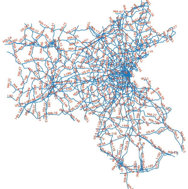
Figure 1: All available road segments in Eastern Massachusetts (from [30]).

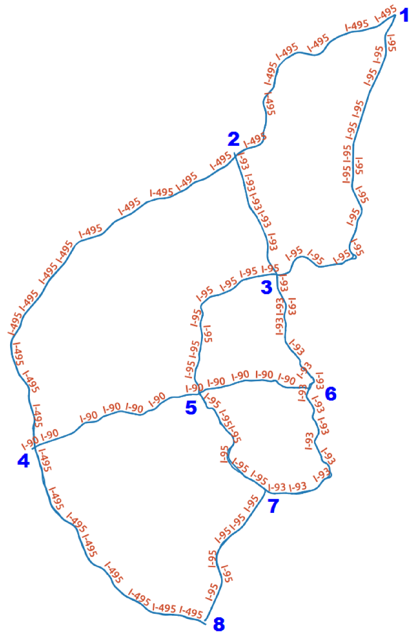
(a)

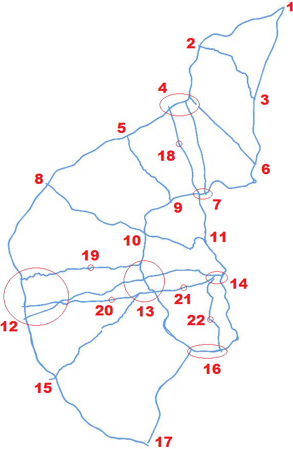
(b)

Figure 2: (a) An interstate highway sub-network of EMA ($\mathcal{I}_{1}$) (the blue numbers indicate node indices); (b) An extended highway sub-network of EMA ($\mathcal{I}_{2}$) (the red numbers indicate node indices). (See [35] for the correspondences between nodes and link indices.)

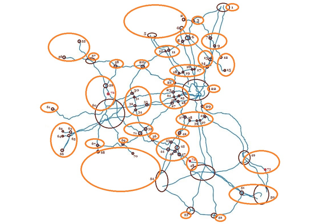
Figure 3: A wider EMA highway subnetwork ($\mathcal{I}_{3}$); details on the correspondences between nodes and link indices are in [35]. (“nodes:zone” pairs – {1}: Seabrook (NH); {2, 4, 5}: NH; {3}: Haverhill; {6, 8}: Lawrence; {7, 9}: Georgetown; {10, 11}: Lowell; {12, 15}: Salem; {13, 14}: Peabody; {16, 17, 18, 19}: Burlington; {20}: Littleton; {21}: Lexington; {22}: Boston; {23, 24, 25, 26, 27, 28}: Waltham; {29}: Quincy; {30, 31, 32, 33, 34}: Marlborough/Framingham; {35, 71}: Milford; {36}: Franklin; {37, 38, 39, 40, 41}: Westwood/Quincy; {42}: Dedham; {43, 44, 45, 46, 47}: Foxborough; {48, 74}: Taunton; {49, 73}: Plymouth; {50, 51}: Cape Cod; {52}: Dartmouth; {53}: Fall River; {54, 68, 70}: RI; {55, 56}: VT; {57}: Westminster; {58}: Leominster; {59, 60, 72}: Worcester; {61}: Amherst; {62, 63, 64, 65, 66}: CT; {67}: Webster; {69}: Uxbridge.)

4.2 Preprocessing

In [30] and [31] we investigate two relatively small subnetworks (denoted by $\mathcal{I}_{1}$ and $\mathcal{I}_{2}$ and shown in Figs. 2(a) and 2(b), respectively) of the EMA road network. Here, we further consider a much larger subnetwork (denoted by $\mathcal{I}_{3}$ and shown in Fig. 3). Performing similar preprocessing procedures as those in [30, 31], we end up with traffic flow data (Wardrop equilibria) and road (link) parameters (flow capacity and free-flow travel time) for the three subnetworks $\mathcal{I}_{1}$, $\mathcal{I}_{2}$, and $\mathcal{I}_{3}$, where $\mathcal{I}_{1}$ contains only interstate highways, $\mathcal{I}_{2}$ also contains state highways, and $\mathcal{I}_{3}$ covers a much wider area of EMA. Note that $\mathcal{I}_{1}$ (resp., $\mathcal{I}_{2}$, $\mathcal{I}_{3}$) consists of 8 (resp., 22, 74) nodes and 24 (resp., 74, 258) links. Assuming that each node could be an origin and a destination, then there are $8\times(8-1)=56$ (resp., $22\times(22-1)=462$) OD pairs in $\mathcal{I}_{1}$ (resp., $\mathcal{I}_{2}$). For $\mathcal{I}_{3}$, we simplify the analysis by grouping nodes within the same area, assigning them the same zone label, thus obtaining 34 zones (as opposed to 74 nodes). Assuming that each zone could be an origin and a destination, then there are $34\times(34-1)=1122$ OD pairs in $\mathcal{I}_{3}$. It is worth pointing out that nodes 18, 19, 20, 21, and 22 (resp., 72, 73, and 74) in $\mathcal{I}_{2}$ (resp., $\mathcal{I}_{3}$) are introduced for ensuring the identifiability of the OD demand matrices. More specifically, to “recover” uniquely an OD demand matrix from observed link flow data, the link-route incidence matrix ${\mathbf{A}}$ is required to satisfy certain structural properties; see [26, Lemma 2].

4.3 Estimating initial OD demand matrices

Operating on $\mathcal{I}_{1}$, we solve the QP (P1) (cf. (13)) and the QCP (P2) (cf. (14)) using data corresponding to five different time periods (AM, MD (middle day), PM, NT (night), and WD (weekend)) of four months (Jan., Apr., Jul., and Oct.) in 2012, thus obtaining 20 different OD demand matrices for these scenarios. Expanding each and every of the 20 OD demand matrices of $\mathcal{I}_{1}$ by setting the demand for any OD pair that belongs to $\mathcal{I}_{2}$ but does not belong to $\mathcal{I}_{1}$ to zero, we obtain “rough” initial demand matrices for $\mathcal{I}_{2}$.

On the other hand, for the much larger subnetwork $\mathcal{I}_{3}$, to obtain initial OD demand matrices corresponding to the same 20 scenarios, we perform a different simplification procedure. In particular, we only consider the shortest route for each OD pair of $\mathcal{I}_{3}$, thus leading to a deterministic route choice matrix ${\mathbf{P}}$ and significantly reducing the number of decision variables in the QCP (P2).

As noted in [30], the GLS method assumes the traffic network to be uncongested. It follows, that the estimated OD demand matrices for non-peak periods (MD/NT/WD) are relatively more accurate than those for peak periods (AM/PM). After obtaining estimates for travel latency cost functions in Sec. 4.4, based on the observed Wardrop flows and the initial estimates for the OD demand matrices, we will conduct demand adjustment procedures for $\mathcal{I}_{2}$ and $\mathcal{I}_{3}$ in Sec. 4.5.

4.4 Cost function estimation and sensitivity analysis

First, to validate the effectiveness and efficiency of the cost function estimator (12), we conduct numerical experiments over the Anaheim benchmark network [37], whose ground truth cost functions, OD demand matrices, and all necessary road parameters are available. Next, operating on $\mathcal{I}_{1}$ using the flow data and the OD demand matrices obtained in Secs. 4.2 and 4.3 respectively, we estimate the travel latency cost functions, $f(\cdot)$ in particular, for 20 different scenarios, via the estimator (12), by solving the QP invVI-2 accordingly. As in [30], to make the estimates reliable, for each scenario, we perform a 3-fold cross-validation. Note that [30] applied a different estimator, which is numerically not as stable.

We assume that such estimates for $f(\cdot)$, as obtained from $\mathcal{I}_{1}$, can be shared by all the three subnetworks $\mathcal{I}_{1}$, $\mathcal{I}_{2}$, and $\mathcal{I}_{3}$; this makes sense, because the function $f(\cdot)$ is common for all links and, when estimating it through $\mathcal{I}_{1}$, we have already made use of a large amount of data (note that there are 24 links in $\mathcal{I}_{1}$ and the flow data and the corresponding OD demand matrices that we use have covered $120$ different time instances for each of the 20 scenarios; for details, see [35]).

To illustrate our method of analyzing sensitivities for the TAP formulation (2), we again conduct numerical experiments on $\mathcal{I}_{1}$. In particular, we investigate a scenario corresponding to the AM peak period of April 2012.

4.5 OD demand adjustments

First, we demonstrate the effectiveness of Alg. 1 using the Anaheim benchmark network. Then, assuming the per-road travel latency cost functions are available (we take the travel latency cost functions derived from $\mathcal{I}_{1}$ as in Sec. 4.4), we apply Alg. 1 to $\mathcal{I}_{2}$, which contains $\mathcal{I}_{1}$ as one of its representative subnetworks. Note that the main difference between $\mathcal{I}_{1}$ and $\mathcal{I}_{2}$ is the modeling emphasis; specifically, $\mathcal{I}_{1}$ only takes account of interstate highways, while $\mathcal{I}_{2}$ also encompasses state highways, thus containing more details of the real road network of EMA. We can think of $\mathcal{I}_{1}$ as a “landmark” subnetwork of $\mathcal{I}_{2}$. Based on the initially estimated demand matrices for $\mathcal{I}_{1}$, we will implement the following generic demand-adjusting scheme so as to derive the OD demand matrices for $\mathcal{I}_{2}$.

Given a network ($\mathcal{I}_{2}$ in our case) of any size we can select its “landmark” subnetworks ($\mathcal{I}_{1}$ in our case) (based on the information of road types, pre-identified centroids, etc.) with acceptably smaller sizes; say we end up with $N$ ($N=1$ in our case) such subnetworks. Then, for each subnetwork, we estimate its demand matrix by solving sequentially the QP (P1) and the QCP (P2) (cf. Sec. 4.3). Setting the demand for any OD pair not belonging to this subnetwork to zero, we obtain a “rough” initial demand matrix for the entire network ($\mathcal{I}_{2}$ in our case). Next, we take the average of these initial demand matrices. Finally, we adjust the average demand matrix based on the flow observations of the entire network.

Next, taking again the travel latency cost functions derived from $\mathcal{I}_{1}$, we apply Alg. 1 to $\mathcal{I}_{3}$, based on the initial OD demand matrices estimated from $\mathcal{I}_{3}$ (see Sec. 4.3) and the Wardrop flows inferred from $\mathcal{I}_{3}$ (see Sec. 4.2).

As noted in Remark 1, the reason for not directly solving (P1) and (P2) for the larger networks ($\mathcal{I}_{2}$ and $\mathcal{I}_{3}$ in our case) is that there are too many decision variables in (P2) and this would lead to numerical difficulties.

4.6 PoA evaluation and meta analysis

We calculate the PoA values for $\mathcal{I}_{2}$ and $\mathcal{I}_{3}$ for the PM period of April 2012. For each day, in (24) we take the average observed link flows over the PM period as the “user flows,” and obtain the “social flows” by solving the NLP (23) using the estimated cost functions and demand matrix exclusively for the PM period. To solve (23), we use the IPOPT solver [38] which implements a primal-dual interior point method [39].

To better understand the performance of the road network under the user-centric vs. the system-centric routing policy, we conduct a meta analysis on $\mathcal{I}_{3}$. In particular, under the two policies, we compare congestion for various zones of the network, the maximum/minimum link flows, and link-specific congestion.

5 Numerical Results

For economy of space, we will not show the detailed results for the initial estimation of OD demand matrices. However, we report in Tab. 1 the entries of the route choice probability matrix ${\mathbf{P}}$ derived for $\mathcal{I}_{1}$ for some specific OD pairs (the complete results can be found in [35]). It is seen from Tab. 1 that we cannot always expect a higher probability for a shorter/faster route; randomness exists. However, this is not necessarily counterintuitive, because the selected routes for the same OD pair have close lengths/travel times. We note here that when identifying (and refining) the feasible routes for each OD pair of $\mathcal{I}_{1}$, we consider at most three shortest routes (ranked #1-#3) and discard all the routes with a length larger than that of the shortest route (ranked #1) by more than $50\%$. Note also that since this initial OD estimation procedure does not involve real-time updates of traffic conditions, we may use either travel times or lengths as weights for links in the graph model.

Table 1: Selected route choice analysis results for $\mathcal{I}_{1}$ (corresponding to the PM peak period of April 2012).

OD pair	refined feasible route	route length (in miles)	free-flow travel time (in hours)	route choice probability
(1, 8)	$1\to 2\to 3\to 5\to 7\to 8$ $1\to 3\to 5\to 7\to 8$ $1\to 2\to 3\to 6\to 7\to 8$	74.2072 74.6696 74.8692	1.0235 1.0297 1.0522	0.3265 0.3394 0.3341
(2, 4)	$2\to 4$ $2\to 3\to 5\to 4$ $2\to 3\to 6\to 5\to 4$	37.6346 43.4554 50.7995	0.5123 0.6010 0.7274	0.8274 0.1004 0.0722
(3, 5)	$3\to 5$ $3\to 6\to 5$	16.2154 23.5596	0.2262 0.3526	0.8375 0.1625
(8, 3)	$8\to 7\to 5\to 3$ $8\to 7\to 6\to 3$ $8\to 7\to 5\to 6\to 3$	43.3260 43.4313 50.2382	0.6065 0.6310 0.7308	0.4364 0.3022 0.2614

In the following, we will focus on presenting the results for the estimates of the travel latency cost functions (derived for the Anaheim benchmark network and $\mathcal{I}_{1}$), the demand adjustment procedure (derived for the Anaheim benchmark network; note that we will not show the detailed demand adjustment results for $\mathcal{I}_{2}$ and $\mathcal{I}_{3}$, because we do not have the ground truth for a comparison), the PoA evaluations (derived for $\mathcal{I}_{2}$ and $\mathcal{I}_{3}$), the sensitivity analysis (derived for $\mathcal{I}_{1}$), and the meta analysis (derived for $\mathcal{I}_{3}$).

5.1 Results from estimating the cost functions

5.1.1 Results for the Anaheim benchmark network

The Anaheim network contains 38 zones (hence $38\times(38-1)=1406$ OD pairs), 416 nodes, and 914 links. The ground truth $f\left(\cdot\right)$ is taken as $f\left(z\right)=1+0.15z^{4},\,z\geq 0$. Fig. 4 shows the estimation results for $f(z)$ by solving invVI-2 corresponding to different parameter settings. In particular, Fig. 4(a) shows the curves of the ground truth $f(z)$ and the estimator $\hat{f}(z)$ corresponding to $n$ taking values from $\{3,4,5,6\}$ while keeping $c$ and $\gamma$ fixed to 1.5 and 0.01 respectively; it is seen that except for the case $n=3$, all estimation curves are very close to the ground truth. Note that the ground truth $f(z)$ is a polynomial function with degree 4, which is greater than 3. This suggests the use of a value $n\geq 4$ in recovering the cost function $f(\cdot)$. The intuition here is that we can use a higher order polynomial with appropriate coefficients to approximate a lower order polynomial, but not vice versa. Fig. 4(b) shows the curves of the ground truth $f(z)$ and the estimator $\hat{f}(z)$ corresponding to $c$ taking values from $\{0.5,1.0,1.5\}$ while keeping $n$ and $\gamma$ fixed to 6 and 1.0 respectively; it is seen that except for the case $c=0.5$, the estimation curves are very close to the ground truth. This suggests that setting $c$ reasonably larger should give better estimation results. Fig. 4(c) plots the curves of the ground truth $f(z)$ and the estimator $\hat{f}(z)$ corresponding to $\gamma$ taking values from $\{0.01,0.1,1.0,10.0,100.0\}$ while keeping $n$ and $c$ fixed to 5 and 1.5 respectively; it is seen that as $\gamma$ is set smaller and smaller, the estimation curve gets closer and closer to the ground truth. This suggests that choosing a smaller regularization parameter $\gamma$ should give tighter estimation results in terms of data reconciling.

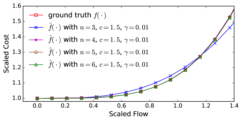
(a) Vary $n$ ($c$ and $\gamma$ fixed).

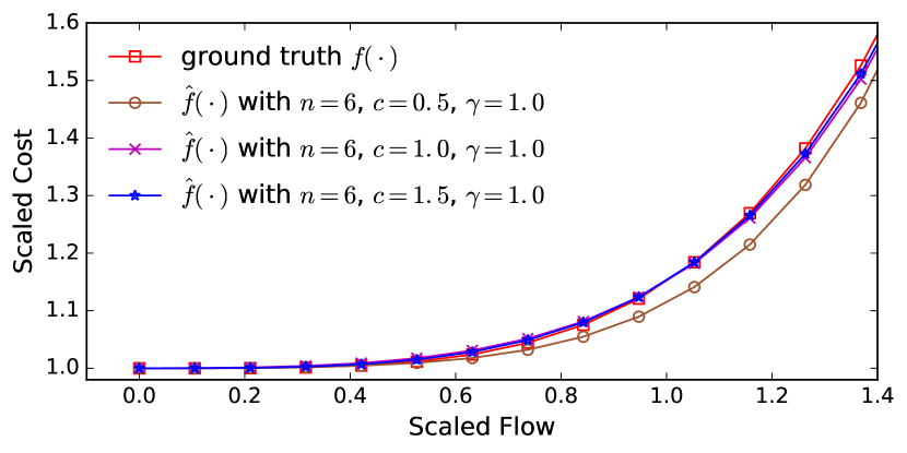
(b) Vary $c$ ($n$ and $\gamma$ fixed).

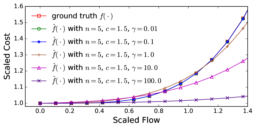
(c) Vary $\gamma$ ($n$ and $c$ fixed).

Figure 4: Estimations for cost function $f(\cdot)$ by solving invVI-2 corresponding to different parameter settings (Anaheim).

5.1.2 Results for $\mathcal{I}_{1}$

We show the comparison results of the cost functions in Fig. 5, where in each sub-figure, we plot the curves of the estimated $f(\cdot)$ corresponding to five different time periods. For economy of space, we will not list the parameter setting details of $n$, $c$, and $\gamma$, which were selected by conducting a 3-fold cross-validation.

We observe from Figs. 5(a)-5(d) that the costs for peak periods (AM/PM) are more sensitive to traffic flows than for non-peak periods (MD/NT/WD). This can be explained as follows: during rush hour, it is very common for vehicles to pass through a congested road network while during non-rush hour, drivers mostly enjoy an uncongested road network.

In addition, it is seen that, for different months, the cost curves for non-peak periods differ more significantly than for peak periods. Aside from the observation and modeling errors, this can also be explained by seasonal traveling patterns.

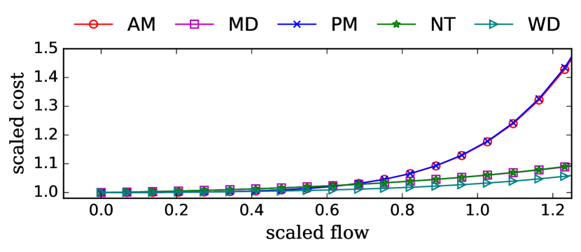
(a) Jan.

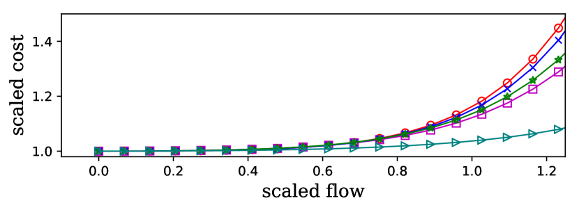
(b) Apr.

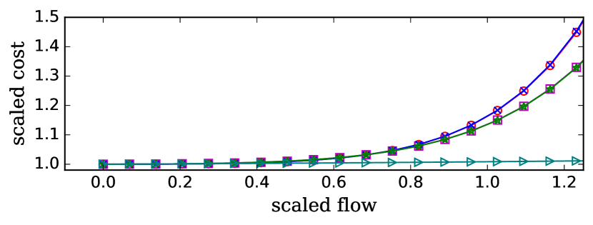
(c) Jul.

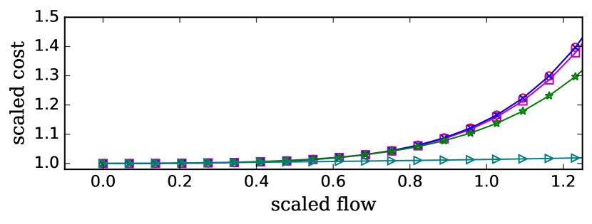
(d) Oct.

Figure 5: Estimates for $f(\cdot)$ corresponding to different time periods (AM, MD (middle day), PM, NT (night), WD (weekend)), derived from data over $\mathcal{I}_{1}$ for 2012.

5.2 Results from OD demand adjustment

We now present the OD demand adjustment results from the Anaheim network. For each OD pair, the initial demand is taken by scaling the ground truth demand using a random factor with uniform distribution over $[0.8,1.2]$. The ground truth $f\left(\cdot\right)$ is taken as $f\left(z\right)=1+0.15z^{4},\;\forall z\geq 0$, and is assumed directly available. When implementing Alg. 1, we set $\gamma_{1}=0$, $\gamma_{2}=1$, $\rho=2$, $T=10$, $\varepsilon_{1}=0$, and $\varepsilon_{2}=10^{-20}$. Fig. 6(a) shows that, after 7 iterations, the objective function value of the BiLev (15) has been reduced by more than $50\%$. Fig. 6(b) shows that, the distance between the adjusted demand and the ground truth demand keeps decreasing with the number of iterations, and the distance changes very slightly, meaning the adjustment procedure does not alter the initial demand much. Note that in Fig. 6(a), the vertical axis corresponds to the normalized objective function value of the BiLev, i.e., $F({\mathbf{g}}^{l})/F({\mathbf{g}}^{0})$ and, in Fig. 6(b), the vertical axis denotes the normalized distance between the adjusted demand vector and the ground truth, i.e., $\|{\mathbf{g}}^{l}-{\mathbf{g}}^{*}\|/\|{\mathbf{g}}^{*}\|$, where ${\mathbf{g}}^{*}$ is the ground-truth demand vector.

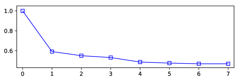
(a) $F({\mathbf{g}}^{l})/F({\mathbf{g}}^{0})$ vs. # of iterations.

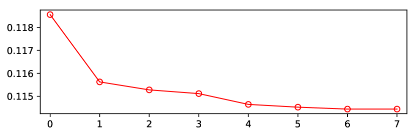
(b) $\|{\mathbf{g}}^{l}-{\mathbf{g}}^{*}\|/\|{\mathbf{g}}^{*}\|$ vs. # of iterations.

Figure 6: Key quantities vs. # of iterations (Anaheim).

5.3 Results for PoA evaluation

After implementing the demand adjusting scheme, we obtain the demand matrices for $\mathcal{I}_{2}$ and $\mathcal{I}_{3}$ on a daily-basis, as opposed to those for $\mathcal{I}_{1}$ on a monthly-basis. Note that, even for the same period of a day and within the same month, slight demand variations among different days are possible; thus, our PoA results for $\mathcal{I}_{2}$ and $\mathcal{I}_{3}$ would be more accurate than those for $\mathcal{I}_{1}$ (shown in [30]).

The PoA values for $\mathcal{I}_{2}$ shown in Fig. 7(a) have larger variations than those for $\mathcal{I}_{1}$ in [30] and for $\mathcal{I}_{3}$ shown in Fig. 7(b); some are closer to 1 but some go beyond 2.2, meaning we have larger potential to improve the road network. It is also seen that, although $\mathcal{I}_{2}$ is extracted from $\mathcal{I}_{3}$, there is no obvious correlation between the PoA values estimated for $\mathcal{I}_{2}$ and $\mathcal{I}_{3}$. To explain this, one should notice the fact that $\mathcal{I}_{2}$ is only a small subnetwork of $\mathcal{I}_{3}$, where the latter contains many more nodes/links/OD pairs (see Figs. 2(b) and 3). Specifically, in Fig. 3 many more links have been added which significantly alter the feasible routing patterns relative to Fig. 2(b). Thus, even though there may be correlations at the individual link flow level, once we add links and then aggregate over all links, any correlation is likely weakened or lost. Moreover, the social optimization problems solved to obtain the denominator of the PoA ratio in (24) are very different since the subnetwork topologies are different. However, when taking the average of the PoA values for all 30 days of Apr. 2012, all $\mathcal{I}_{1}$, $\mathcal{I}_{2}$, and $\mathcal{I}_{3}$ result in an average PoA approximately equal to 1.5, meaning we can gain an efficiency improvement of about 50%; thus, the results are consistent.

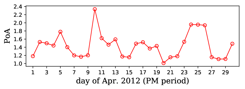
(a) for $\mathcal{I}_{2}$

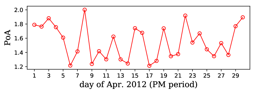
(b) for $\mathcal{I}_{3}$

Figure 7: Daily PoAs for $\mathcal{I}_{2}$ and $\mathcal{I}_{3}$ (PM period for Apr. 2012).

5.4 Results from sensitivity analysis

Investigating the AM peak period of Apr. 2012 for $\mathcal{I}_{1}$, instead of directly applying the formulae (27) and (28), we calculate the two quantities defined in (29) and (30), and plot the results in Fig. 8, where the blue (resp., red) curve indicates the quantity $\Delta V\left({{{\mathbf{t}}^{0}},{\mathbf{m}};\Delta t_{a}^{0}}\right)$ (resp., $\Delta V\left({{{\mathbf{t}}^{0}},{\mathbf{m}};\Delta m_{a}}\right)$) for each and every link of $\mathcal{I}_{1}$. It is seen from Fig. 8 that the largest four values of $\Delta V\left({{{\mathbf{t}}^{0}},{\mathbf{m}};\Delta t_{a}^{0}}\right)$ (resp., $\Delta V\left({{{\mathbf{t}}^{0}},{\mathbf{m}};\Delta m_{a}}\right)$) correspond to links 10, 19, 9, and 5 (resp., 10, 19, 9, and 1). This suggests that, during the AM peak period of Apr. 2012, the transportation management department could have most efficiently reduced the objective function value of the TAP (2), thus mitigating congestion, by taking actions with priorities on these links (e.g., improving road conditions to reduce the free-flow travel time for links 10, 19, 9, and 5, and increasing the number of lanes to enlarge the flow capacity for links 10, 19, 9, and 1).

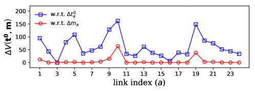
Figure 8: Sensitivity analysis (finite difference approximation) results for $\mathcal{I}_{1}$; AM period of Apr. 2012.

5.5 Results from meta analysis

We conduct meta analysis for $\mathcal{I}_{3}$, under the user-centric routing policy vs. the system-centric one. Our analysis includes the zone costs, the maximum/minimum link flows, and the link-specific congestion.

5.5.1 Meta analysis for zone costs

Let $\mathcal{A}_{3}^{i}$ denote the set of links related to zone $i$ of $\mathcal{I}_{3}$ (each link in $\mathcal{A}_{3}^{i}$ has at least one node contained in zone $i$). Then, the total users’ travel latency cost for zone $i$ is defined as

$${C_{i}}=\sum\limits_{a\in{\mathcal{A}_{3}^{i}}}{{{x_{a}}}{{t_{a}}\left(x_{a}\right)}}.$$

We consider two scenarios, one corresponding to the PM peak period of a typical weekday (Wednesday, 4/18/2012) and the other the PM period of a typical weekend (Sunday, 4/15/2012). The zone costs under the user-centric (resp., system-centric) routing policy are visualized in Fig. 9(a) (resp., 9(b)). Three observations can be made: (i) Overall, most zone costs would be reduced when switching from the user-centric routing policy to the system-centric one. (ii) In general, the zone costs for weekends are less than their counterparts for weekdays; this is consistent with intuition. (iii) The decrease seems more consistent for all zones during weekends than during weekdays, suggesting it is easier to optimize the network during weekends; this is again consistent with intuition.

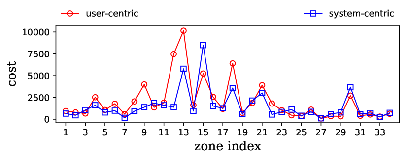
(a) weekday (4/18/2012)

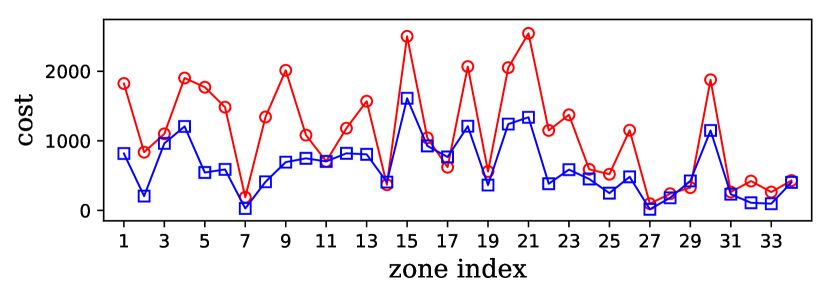
(b) weekend (4/15/2012)

Figure 9: Zone costs under user-centric vs. system-centric routing policy (PM period of Apr. 2012).

5.5.2 Meta analysis for maximum/minimum link flows

The maximum/minimum link flows for the PM peak period of each and every day of Apr. 2012 are plotted in Fig. 10(a), and the corresponding link indices are shown in Fig. 10(b). A major observation, based on Fig. 10(a), is that the maximum link flow values would increase for most of the days when switching the routing policy from the user-centric one to the system-centric one, which is desirable. In addition, it is seen that, among the entire month (April 2012), both the maximum link flows under the two routing policies have a weekly periodic distribution; this is consistent with intuition.

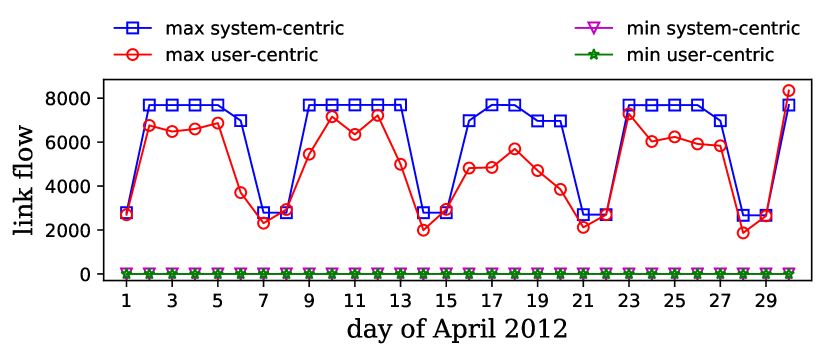
(a)

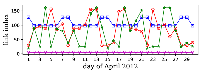
(b)

Figure 10: Maximum/minimum link flows and the corresponding link indices under user-centric vs. system-centric routing policy (PM period of Apr. 2012).

5.5.3 Meta analysis for link congestion

For any given link $a$, we define its Congestion Metric (CM) [40] as the ratio of the travel time to free-flow travel time:

$${\text{CM}_{a}}\stackrel{{\scriptstyle\text{def}}}{{=}}\frac{{{t_{a}}\left({{x_{a}}}\right)}}{{t_{a}^{0}}}=f\left({\frac{{{x_{a}}}}{{{m_{a}}}}}\right),$$ (31)

where $f(\cdot)$ is the cost function that we have estimated. By this definition, we always have $\text{CM}_{a}\geq 1$.

We first consider a PM peak period scenario for a typical workday (Wednesday, 4/18/2012). The CM values of all the 258 links are plotted in Fig. 11 in a logarithmic scale (base 2). It is seen that, for some links (indexed with 79, 92, and 86) the CM value is significantly higher ($\text{gap}>1$) under the user-centric routing policy than under the system-centric one. There are some links for which we have the opposite, but, overall, the CM peak is reduced under the system-centric policy. We then investigate a PM period scenario for a typical weekend (Sunday, 4/15/2012), and find that all the CM values for this scenario are very close to 1, meaning there was almost no congestion for all links; we have omitted the weekend CM plot for economy of space.

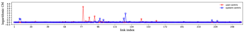
Figure 11: Link congestion under user-centric vs. system-centric routing policy (PM period of 4/18/2012).

6 Strategies for PoA reduction

After quantifying the PoA, a natural question we must answer is the following: How can we reduce the PoA for a given transportation network? We propose three practical strategies for reducing the PoA, especially when $\text{PoA}\gg 1$.

First, by taking advantage of the rapid emergence of Connected Automated Vehicles (CAVs), it has become feasible to automate routing decisions, thus solving a system-centric forward problem (cf. (23)) in which all CAVs (bypassing driver decisions) cooperate to optimize the overall system performance.

Second, we propose a modification to existing GPS navigation algorithms recommending to all drivers socially optimal routes, which could be implemented by making use of (25). In particular, we can solve the user-centric forward problem (2), embedded in a typical GPS navigation application, with $t_{a}(\cdot)$ replaced by $\overline{t}_{a}(\cdot)$, whose common cornerstone part, $f(\cdot)$, is estimated using (12). It is worth pointing out that some existing work simply took $f(\cdot)$ to be the Bureau of Public Roads (BPR)’s [7] empirical polynomial function $f(z)=1+0.15z^{4},\,\forall z\geq 0$, which would not be as accurate.

Finally, our sensitivity analysis results provide the means to prioritize road segments for specific interventions that can mitigate congestion.

7 Conclusions and Future Work

In this paper, we assess the efficiency of transportation networks under a selfish user-centric routing policy as opposed to a socially-optimal system-centric routing policy. To that end, we define and quantify the Price of Anarchy (PoA) and propose possible strategies to reduce it. All the procedures involved are data-driven, thus having the capability of dynamically optimizing any given transportation network (by using the data collected in real-time manner), in terms of reducing the PoA (especially when $\text{PoA}\gg 1$) such that it gets as close to 1 as possible.

We must keep in mind that, due to unavoidable inaccuracies in data and modeling, all the numerical results shown in Sec. 5 are only estimates. In particular, the speed-to-flow conversion model that we use (Greenshield’s model) is a macroscopic model with naturally limited accuracy, the GLS method that we leverage also is based on an approximation, and the MSA subroutine in Alg. 1 is an approximate scheme.

In terms of the computational challenges of our proposed approaches, we encountered numerical difficulties when solving (13) and (14) to obtain OD demands for large-sized (say a network like $\mathcal{I}_{3}$) networks. However, we subsequently developed a simplification procedure by considering only the fastest route for each OD pair, thus successfully resolving this issue. We conducted case studies on a workstation with 24 GB memory and a 12-core Intel Core i5 CPU, and for the largest network ($\mathcal{I}_{3}$) that we investigated, the total CPU time (including estimating OD demands, recovering link latency cost functions, adjusting OD demands, solving for socially-optimal flows, and finally calculating PoA values) is about 10 hours. The total CPU times for $\mathcal{I}_{1}$ and $\mathcal{I}_{2}$ are about 30 minutes and 2 hours, respectively. We note that the most time-consuming task is adjusting OD demands using Alg. 1. However, it is seen that Steps 2-4 of Alg. 1 and the MSA subroutine can easily benefit from parallel computing. Thus, scalability can be further improved through parallel computation. Moreover, following an approach of “divide and conquer,” several decomposition methods could possibly also be leveraged as we move to larger networks; the difficulty lies in how to reasonably “merge” results derived for subnetworks so as to obtain the final result for the whole network.

Our ongoing work includes extending the PoA analysis and reduction framework from single-class to multi-class transportation networks. We have recently obtained results for the multi-class user-centric inverse problem [41], which paves the way for data-driven PoA estimation in these networks. We are also considering alternative models/methods to improve the accuracy in the PoA evaluation. In addition, it is of interest to consider jointly estimating/adjusting the OD demand matrices and recovering the travel latency cost functions.

References

- [1] “World’s population increasingly urban with more than half living in urban areas,” Report on World Urbanization Prospects, United Nations Department of Economic and Social Affairs, July 2014, http://www.un.org/en/development/desa/news/population/world-urbanizatio%n-prospects-2014.html.
- [2] D. Shrank, T. Lomax, and B. Eisele, “The 2011 urban mobility report,” Texas A&M Transportation Institute, Tech. Rep., 2011, https://nacto.org/docs/usdg/2011_urban_mobility_report_schrank.pdf.
- [3] “Economic and environmental of traffic congestion in Europe and the U.S.” INRIX, http://www.inrix.com/economic-environment-cost-congestion/, 2015.
- [4] H. Youn, M. T. Gastner, and H. Jeong, “Price of anarchy in transportation networks: Efficiency and optimality control,” Physical review letters, vol. 101, no. 12, pp. 128 701/1–128 701/4, 2008.
- [5] J. G. Wardrop, “Some theoretical aspects of road traffic research,” Proceedings of the Institution of Civil Engineers, vol. 1, pp. 325–378, 1952.
- [6] P. Patriksson, The traffic assignment problem: models and methods. Utrecht, 1994.
- [7] D. Branston, “Link capacity functions: A review,” Transportation Research, vol. 10, no. 4, pp. 223–236, 1976.
- [8] T. Abrahamsson, “Estimation of origin-destination matrices using traffic counts–a literature survey,” IIASA Interim Report IR-98-021/May, vol. 27, p. 76, 1998.
- [9] S. Bera and K. Rao, “Estimation of origin-destination matrix from traffic counts: the state of the art,” 2011.
- [10] D. Bertsimas, V. Gupta, and I. C. Paschalidis, “Data-driven estimation in equilibrium using inverse optimization,” Mathematical Programming, pp. 1–39, 2015.
- [11] H. Spiess, “A gradient approach for the OD matrix adjustment problem,” Centre de Recherche sur les Transports, Universite de Montreal, no. 693, 1990.
- [12] J. T. Lundgren and A. Peterson, “A heuristic for the bilevel origin–destination-matrix estimation problem,” Transportation Research Part B: Methodological, vol. 42, no. 4, pp. 339–354, 2008.
- [13] S. Pourazarm, C. G. Cassandras, and T. Wang, “Optimal routing and charging of energy-limited vehicles in traffic networks,” International Journal of Robust and Nonlinear Control, vol. 26, no. 6, pp. 1325–1350, 2016.
- [14] J. Alonso, V. Milanés, J. Pérez, E. Onieva, C. González, and T. De Pedro, “Autonomous vehicle control systems for safe crossroads,” Transportation research part C: emerging technologies, vol. 19, no. 6, pp. 1095–1110, 2011.
- [15] J. Lee, B. B. Park, K. Malakorn, and J. J. So, “Sustainability assessments of cooperative vehicle intersection control at an urban corridor,” Transportation Research Part C: Emerging Technologies, vol. 32, pp. 193–206, 2013.
- [16] Y. J. Zhang, A. A. Malikopoulos, and C. G. Cassandras, “Optimal control and coordination of connected and automated vehicles at urban traffic intersections,” in American Control Conference (ACC), 2016. IEEE, 2016, pp. 6227–6232.
- [17] J. Rios-Torres and A. A. Malikopoulos, “A survey on the coordination of connected and automated vehicles at intersections and merging at highway on-ramps,” IEEE Transactions on Intelligent Transportation Systems, vol. 18, no. 5, pp. 1066–1077, 2017.
- [18] S. C. Dafermos and F. T. Sparrow, “The traffic assignment problem for a general network,” Journal of Research of the National Bureau of Standards B, vol. 73, no. 2, pp. 91–118, 1969.
- [19] L. J. LeBlanc, E. K. Morlok, and W. P. Pierskalla, “An efficient approach to solving the road network equilibrium traffic assignment problem,” Transportation Research, vol. 9, no. 5, pp. 309–318, 1975.
- [20] S. C. Dafermos, “The traffic assignment problem for multiclass-user transportation networks,” Transportation science, vol. 6, no. 1, pp. 73–87, 1972.
- [21] A. Nagurney, “A multiclass, multicriteria traffic network equilibrium model,” Mathematical and Computer Modelling, vol. 32, no. 3-4, pp. 393–411, 2000.
- [22] S. Ryu, A. Chen, and K. Choi, “Solving the stochastic multi-class traffic assignment problem with asymmetric interactions, route overlapping, and vehicle restrictions,” Journal of Advanced Transportation, 2015.
- [23] T. L. Friesz, J. Luque, R. L. Tobin, and B.-W. Wie, “Dynamic network traffic assignment considered as a continuous time optimal control problem,” Operations Research, vol. 37, no. 6, pp. 893–901, 1989.
- [24] B. N. Janson, “Dynamic traffic assignment for urban road networks,” Transportation Research Part B: Methodological, vol. 25, no. 2, pp. 143–161, 1991.
- [25] S. Nguyen, “Estimating origin destination matrices from observed flows,” Publication of: Elsevier Science Publishers BV, 1984.
- [26] M. L. Hazelton, “Estimation of origin–destination matrices from link flows on uncongested networks,” Transportation Research Part B: Methodological, vol. 34, no. 7, pp. 549–566, 2000.
- [27] H. Yang, Q. Meng, and M. G. Bell, “Simultaneous estimation of the origin-destination matrices and travel-cost coefficient for congested networks in a stochastic user equilibrium,” Transportation Science, vol. 35, no. 2, pp. 107–123, 2001.
- [28] H. Yang, “Sensitivity analysis for the elastic-demand network equilibrium problem with applications,” Transportation Research Part B: Methodological, vol. 31, no. 1, pp. 55–70, 1997.
- [29] M. Patriksson, “Sensitivity analysis of traffic equilibria,” Transportation Science, vol. 38, no. 3, pp. 258–281, 2004.
- [30] J. Zhang, S. Pourazarm, C. G. Cassandras, and I. C. Paschalidis, “The price of anarchy in transportation networks by estimating user cost functions from actual traffic data,” in Proceedings of IEEE 55th Conference on Decision and Control (CDC), Dec 2016, pp. 789–794.
- [31] ——, “Data-driven estimation of origin-destination demand and user cost functions for the optimization of transportation networks,” in Proceedings of the 20th IFAC World Congress, Toulouse, France, July 9–14 2017, pp. 9680–9685.
- [32] B. Monnot, F. Benita, and G. Piliouras, “How bad is selfish routing in practice?” arXiv preprint arXiv:1703.01599, 2017.
- [33] S. Boyd and L. Vandenberghe, Convex optimization. Cambridge university press, 2004.
- [34] T. Evgeniou, M. Pontil, and T. Poggio, “Regularization networks and support vector machines,” Advances in computational mathematics, vol. 13, no. 1, pp. 1–50, 2000.
- [35] J. Zhang, S. Pourazarm, C. G. Cassandras, and I. C. Paschalidis, “InverseVIsTraffic,” https://github.com/jingzbu/InverseVIsTraffic, 2017.
- [36] Y. Noriega and M. A. Florian, “Algorithmic approaches for asymmetric multi-class network equilibrium problems with different class delay relationships,” https://www.cirrelt.ca/DocumentsTravail/CIRRELT-2007-30.pdf, CIRRELT, 2007.
- [37] H. Bar-Gera et al., “Transportation networks for research,” https://github.com/bstabler/TransportationNetworks, 2017.
- [38] A. Wächter and C. Laird, “Interior Point OPTimizer,” https://en.wikipedia.org/wiki/IPOPT, 2016.
- [39] S. J. Wright, Primal-dual interior-point methods. Siam, 1997.
- [40] M. Aftabuzzaman, “Measuring traffic congestion-a critical review,” in Australasian Transport Research Forum, vol. 30, no. 1, 2007.
- [41] J. Zhang and I. C. Paschalidis, “Data-driven estimation of travel latency cost functions via inverse optimization in multi-class transportation networks,” in Proceedings of the 56th IEEE Conference on Decision and Control, Melbourne, Australia, December 12–16 2017, available in arXiv:1703.04010.