Adapting Sampling Interval of Sensor Networks Using On-Line Reinforcement Learning

Abstract

Monitoring Wireless Sensor Networks (WSNs) are composed of sensor nodes that report temperature, relative humidity, and other environmental parameters. The time between two successive measurements is a critical parameter to set during the WSN configuration because it can impact the WSN’s lifetime, the wireless medium contention and the quality of the reported data. As trends in monitored parameters can significantly vary between scenarios and within time, identifying a sampling interval suitable for several cases is also challenging. In this work, we propose a dynamic sampling rate adaptation scheme based on reinforcement learning, able to tune sensors’ sampling interval on-the-fly, according to environmental conditions and application requirements. The primary goal is to set the sampling interval to the best value possible so as to avoid oversampling and save energy, while not missing environmental changes that can be relevant for the application. In simulations, our mechanism could reduce up to $73\%$ the total number of transmissions compared to a fixed strategy and, simultaneously, keep the average quality of information provided by the WSN. The inherent flexibility of the reinforcement learning algorithm facilitates its use in several scenarios, so as to exploit the broad scope of the Internet of Things.

I Introduction

The broad adoption of wireless sensor nodes for environmental monitoring purposes happened not only because of their capacity of sensing and transmitting (via radio) several environmental parameters but mainly thanks to their low production costs. In fact, their low production costs are a result of limited resources, such as battery and memory, which have boosted lots of research work aimed at extending their lifetime without affecting their most valuable asset: the sensed data.

In monitoring Wireless Sensor Networks (WSNs), the sensor nodes’ sampling interval is crucial for generating high-quality data. The data quality is reduced when the interval between two measurements is not sufficiently short to report significant changes in the monitored parameters, or if it is too brief and report several similar (and, consequently, unimportant) successive values. Furthermore, a sampling interval set under some conditions may occasionally become too short (or too long) within time, due to the environment’s evolution. Additionally, besides the data quality, the sampling interval affects the wireless medium access and stirs up network congestion, end-to-end delays, and sensor nodes’ energy consumption. In conclusion, the sampling interval configuration must focus on the trade-off between data quality and resource savings.

In this work, we propose an on-line sampling interval adaptation scheme. Our mechanism relies on real-time analysis of the data produced by sensor nodes to dynamically adapt the WSN operation to the current environmental conditions. Our primary goal is to guarantee the minimum number of transmissions needed to avoid losing valuable environmental data. To achieve that, we aim to keep the maximum difference between two consecutive measurement values below a threshold, which is set according to the application needs.

We formally represent the scenario of a monitoring WSN through the reinforcement learning model and apply a Q-Learning algorithm to learn the most suitable sampling intervals under different conditions, without an a-priori model of the environment’s evolution. The learning agent may be placed in the cloud, a central gateway or each sensor, according to the resource constraints. The scope of our work is to evaluate the algorithm and observe factors that impact its performance, whereas analyzing the performance difference between centralized and distributed solutions is left for future work.

The rest of the paper is organized as follows: Section II describes the basics of reinforcement learning; Section III enumerates related works that adopted reinforcement learning to optimize sensor networks at different layers, and those that focused on avoiding unnecessary transmissions without losing important changes in the environment; Section IV formulates the problem of adapting the sensor nodes’ sampling interval as a reinforcement learning problem; Section V explains how we generated controlled scenarios and experimental results; Section VI shows experimental results of the reinforcement learning technique applied to real datasets; Section VII shows our conclusions and ideas for future work.

II Background - Reinforcement Learning

Reinforcement Learning (RL) is a machine learning technique that allows an agent to determine automatically a system’s optimal behavior to achieve its goal [1]. Such an optimal behavior is based on the positive and negative feedbacks received from the environment after taking certain actions. Assuming that interactions between the agent and the environment occur at a sequence of discrete time instant $t$, an RL model is defined by:

• a set of possible observations $O$ that the agent may make, such that $o_{t}\in O$ is the observation made at time $t$;

• a set of states $S$, such that the state $s_{t}\in S$ is observed at time $t$;

• a set of actions $A$, such that the action $a_{t}\in A$ is taken at time $t$;

• a state transition function $T(s_{t},a_{t},s_{t+1})$ that calculates the probability of making a transition from $s_{t}$ to $s_{t+1}$ after performing $a_{t}$; and

• a set of rules that determine the scalar immediate reward $r_{t+1}=R(s_{t},a_{t})$, which scales the goodness of taking $a_{t}$ in $s_{t}$.

Each state should satisfy the Markov property, that is, to be independent of any state or action previous to time $t$. An RL agent aims to obtain the maximum long-term reward for a Markov Decision Process environment, even when the model of the environment is unknown or difficult to learn. The strategy adopted to maximize the long-term reward defines the agent’s way of behaving at a certain time and is called a policy.

II-A Q-Learning

Q-Learning is an RL algorithm that does not depend on a state transition function to work. More precisely, the algorithm relies on an optimal action-value function $Q(s,a)$, which value is the estimated reward of executing $a$ in $s$, assuming that the agent will always follow the policy that provides the maximum long-term reward.

At any state $s_{t}$, a selected action $a_{t}$ determines the transition to the state $s_{t+1}$ and the value associated to the pair ($s_{t}$, $a_{t}$) is updated:

$$\begin{split}Q_{t+1}(s_{t},a_{t})=&~{}\alpha\left(r_{t+1}+\gamma\max_{a}Q_{t}(s_{t+1},a)-Q_{t}(s_{t},a_{t})\right)\\ &+Q_{t}(s_{t},a_{t})\text{,}\end{split}$$ (1)

where $s_{t+1}$ and $r_{t+1}$ are the state and reward, respectively, obtained after performing $a_{t}$ in $s_{t}$, the learning rate $\alpha\in[0,1]$ is a positive step-size parameter, and the discount factor $\gamma\in[0,1]$ is used to determine the weight of future rewards. If $\gamma=0$, the agent will behave so as to maximize its immediate reward, even if this would imply a lower long-term return.

By visiting several times each ($s$, $a$) pair, the agent learns which is the action that gives the best long-term reward in each state. Hence, if the number of states is high, the algorithm takes longer and requires more data to find the best action for each state, i.e., to converge. Therefore, it is critical to have a concise representation of the environment, thus to define the set of states according to the goals of the algorithm and do not include unnecessary information. In short, the set of states should illustrate only and all the characteristics that are relevant for the problem under consideration.

III Related Work

Several works have already adopted reinforcement learning techniques at various layers to improve wireless networks’ performance. In [2], the authors proposed a self-adaptive routing framework for wireless mesh networks. Using the Q-Learning algorithm, it was possible, in runtime, to select the most proper routing protocol from a pre-defined set of options and successfully increase the average data throughput in comparison to static techniques. Other examples of the use of reinforcement learning techniques in sensor networks include locating mobile sensor nodes [3] and aggregating sensed data [4].

WSNs are mainly composed of wireless sensor nodes that make measurements and transmit them to a Gateway (GW). There are many solutions to reduce their number of transmissions, which include clustering, data aggregation, and data prediction. In [5], the authors suggest that future measurements can be predicted by sensor nodes and GWs. Therefore, sensor nodes only transmit a measurement if they observe that the prediction is not correct, i.e., the real measurement differs by more than a certain threshold from the predicted value. The success of this technique highly depends on the capacity of the sensor nodes to compute efficient prediction methods that will accurately predict future values. However, sensor nodes usually have very limited computing capacities and must rely on GWs to regularly generate and transmit new predictions. Moreover, GWs and sensor nodes must share the same knowledge, which requires additional control messages and reduces the benefit of decreasing measurement transmissions, especially if predictions are not sufficiently accurate.

In [6], the authors propose an approach to answering queries in GWs without fetching the data directly from sensor nodes. The Principal Component Analysis method was used to analyze historical data and select only the sensor nodes that measured most of the variance observed in the environment. This technique reduced the workload of the sensor nodes and reduced up to $50\%$ the number of transmissions, according to the results obtained from experiments in real testbeds. However, the authors do not define how the environment’s evolution would be addressed. For example, if the temperature varies more often during the day, it would be necessary more measurements from more sensor nodes during these hours to build datasets that reliably describe the environment.

Our work does not necessarily rely on the computational capacity of sensor nodes or GWs because the incorporation of WSNs into the IoT allows the use of external entities and cloud computing services that can perform powerful machine learning techniques over sensed data if needed [7]. To the best of our knowledge, this is the first approach that dynamically adapts the sampling interval of the sensor nodes based on a reinforcement learning technique.

IV Adaptive sampling as a reinforcement learning problem

In this Section, we formulate the adaptive sampling interval problem as a reinforcement learning problem. For this work, we take as a reference the real scenario of a WSN with several nodes measuring temperature values in an office [8]. From this real dataset, we use a sub-set of measurements in the preliminary analysis presented in Section IV-B, and a different sub-set in the performance evaluation in Section VI (missing values were interpolated and added to a small white noise). Moreover, as the sensors of this scenario were set to sample temperature nearly every $30$ seconds, we set this as the shortest sampling interval and let the range of possible sampling intervals be (i) $\mathbf{30}$seconds; (ii) $\mathbf{60}$seconds; (iii) $\mathbf{120}$seconds; or (iv) $\mathbf{240}$seconds.

A valuable adaptive sampling algorithm should systematically set up the most proper sampling interval so as to guarantee the best quality-resource trade-off under the current environmental conditions. As for the quality, we define the goal of the agent in terms of an accepted threshold $\tau$. The algorithm should avoid that the absolute difference between consecutive measurements exceeds a pre-defined value ($\tau$), which is configured according to the monitoring application requirements. Meanwhile, higher sampling intervals are preferred to reduce the number of transmissions and, consequently, the energy consumption in sensor nodes.

In our experiments, we consider the number of transmissions as a general measure of resource optimization, which is also valuable in scenarios with energy constraints. For space limitation, we can not include other metrics that may be more relevant in specific scenarios, such as the energy saved by reducing report transmissions or by increasing the idle time of the sensor nodes.

IV-A Observations

First, we define wireless sensor nodes as the source of the observations made by an agent. Observations may vary, among other parameters, between temperature, relative humidity and solar radiation. In our scenario example, an observation $o_{t}$ is the temperature measured at time $t$.

Factor	Description
Quality ($q$)	$q\triangleq|o_{t}-o_{t-1}|\leq\tau\therefore q\in\{\text{true},\text{false}\}$
Hour of the day ($h$)	$h\in[0,1,\ldots,23]$
Is it working hour? ($\omega$)	$\omega\triangleq h\geq 7~{}\text{and}~{}h\leq 18\therefore\omega\in\{\text{true},\text{false}\}$
Day of the week ($d$)	$d\in\{\text{Monday},~{}\text{Tuesday},~{}\ldots,~{}\text{Sunday}\}$
Is it weekend? ($e$)	$e\triangleq d\in\{\text{Sat.},~{}\text{Sun.}\}\therefore e\in\{\text{true},\text{false}\}$
Sampling interval ($s$)	$s\in\{30,60,120,240\}$ seconds
Node ID ($i$)	Individual sensor node identification.

TABLE I: Factors that can impact the quality of measurements.

IV-B States

To properly define the set of possible states, we make a preliminary evaluation of part of the data collected by the WSN, to identify characteristics that have a high correlation with our goal. Such characteristics are transformed into predictors, and a Random Forest [9] is built to classify in which periods of time each sampling interval would make consecutive measurements that differ by less than $\tau$.

In this process, we use the data from three different sensor nodes sampled every $30$ seconds for three days. To simulate different sampling intervals, we removed intermediate measurements and, after analyzing the generated data, the value of $\tau$ was set to $0.02^{o}$C. Using this value, a sampling interval of $120$ seconds would be sufficient to observe a difference of less than $\tau$ in nearly one-half of the time. Furthermore, sampling intervals of $30$, $60$ and $240$ seconds would be sufficient to observe a difference of less than $\tau$ in, respectively, approximately $73.2\%$, $59.2\%$ and $26.1\%$ of the time. Note that we do not expect to measure fast enough to make all measurements differ by less than $\tau$, but we know that there are many cases in which sensors do not have to sample every $30$ seconds to achieve it.

Finally, we annotate each measurement with the characteristics shown in Table I and build a Random Forest to observe what are the most relevant factors to predict if a measurement will differ by less than $\tau$ from the previous one (i.e., $q=\text{true}$). Based on the results obtained using the Random Forest algorithm and considering the importance of keeping a small number of states, we defined the set of states for our RL model as a combination of quality, sampling interval and a verification of whether it is a working hour or not (see Table I) . Thus, each state is defined by a tuple: $\{q,s,\omega\}$. In short, as we are looking for states that will be used by different sensor nodes, we ignored any factor that was less important than the node ID to predict the quality of the measurements and those that would represent a significant increase in the number of states, such as the hour of the day.

IV-C Actions and transitions

In the adaptive sampling interval problem, actions are used to control the sensor nodes’ sampling interval. An action can be specific, such as “set the sampling interval to 30 seconds”, or more abstract, like “increase the sampling interval” requiring the new sampling interval to be calculated based on the last value set. To avoid abrupt changes provoked by occasional outliers and noise in the data, we adopt only “smooth” actions, i.e., they only move to neighboring states. Therefore, an action $a$ can take one of the following values: (i) increase the sampling interval; (ii) keep the sampling interval; or (iii) reduce the sampling interval.

IV-D Reward

A reward is a mathematical representation of the gains obtained after reacting to the environment with a particular action. In our case, after changing the sampling interval to a new value, while in $s$. As the reward defines the target of the algorithm, in our problem, it should ensure that the difference between consecutive measurements is less than $\tau$, while not oversampling.

The algorithm adopted for the reward is based on the rate of transmissions avoided. For instance, if the sampling interval is $120$ seconds, the sensor node is transmitting four times less than if it was $30$ seconds. In this case, therefore, the original reward would be set to four. Then, if the absolute difference between two consecutive measurements ($\delta$) is less than $\tau$, we assume that the sampling interval is small enough to avoid losing significant changes in the environment and take the original reward. If $\delta$ is smaller than one-half of $\tau$, the sampling interval might be doubled, so we multiply the original reward by $\mathbf{1.5}$. Otherwise, if $\delta$ is greater than $\tau$, the sampling interval is too long, and the reported data may be missing important changes in the environment. In this case, we multiply the original reward by$~{}\mathbf{-1}$.

V Synthetic scenarios

To check the feasibility of using RL as a means of intelligently adapting sampling intervals, we simulate its use in artificial and realistic scenarios. In this Section, we present the simplest scenarios, using synthetic data with evident characteristics, such as vast and significant (versus small and negligible) variations in a short period. Having control over the data characteristics allows us first to verify if the RL algorithm decides for the most proper actions in different scenarios. Later, we analyze the impact of the values of learning rate $\alpha$ and discount factor $\gamma$ on the time that the agent needs to reach the most proper state when it occurs.

Learning rate $\alpha$	Discount factor $\gamma$	Convergence time (s)	% of wrong decisions	% of measurements over $\tau$
0.9	0.1	1013.00	4.79	2.31
0.8	0.2	1050.32	6.11	4.38
0.8	0.1	1088.01	8.36	1.80
0.8	0.4	1163.05	13.46	8.80
0.8	0.5	1640.30	12.82	10.79
0.9	0.2	1920.57	11.57	3.65
0.5	0.2	18330.53	25.39	10.89
0.9	0.4	18457.82	19.90	4.63
0.6	0.1	21922.80	18.47	5.47
0.9	0.5	23512.98	20.68	4.34

TABLE II: Simulations over the Controlled datasets: average convergence times and percentage of wrongly taken decisions by each combination of $\alpha$ and $\gamma$. These values are sorted by the lowest convergence times.

V-A Fixed expectations

We generated six synthetic scenarios in which we have control about the sampling intervals that the algorithm should set. In these datasets, the difference between consecutive measurements is proportional to $\tau$. For instance, if the difference between two consecutive measurements made over a period of $60$ seconds is always smaller than $\tau$, setting the sampling interval to $30$ or $60$ seconds is sufficient to satisfy the requirements of quality. However, setting the sampling interval to $60$ seconds would be preferred, because it reduces the number of transmissions, in comparison with the $30$ seconds interval.

In the Controlled 30 dataset, the difference between subsequent measurements made over an interval of $30$ seconds between each other is always $110\%$ of $\tau$. In practice, even the smallest sampling interval ($30$ seconds) is not sufficient to provide measurements in which consecutive values differ by less than $\tau$. Therefore, the agent must define the ideal sampling interval as $30$ seconds to reduce as much as possible the quality loss. Note that in this particular scenario, a difference between subsequent measurements higher than the maximum threshold is unavoidable. Therefore, we do not consider this dataset when reporting the percentage of measurements over $\tau$.

In the Controlled 60, Controlled 120 and Controlled 240 datasets, the difference between subsequent measurements made at an interval of $30$ seconds between each other is respectively $47.5\%$ $23.75\%$ and $10\%$ of $\tau$. Hence, $60$, $120$ and $240$ seconds are respectively the largest possible sampling intervals such that the sensor node will never report a difference greater than $\tau$. Hence, the agent must define the ideal sampling interval respectively to $60$, $120$ and $240$ seconds in each scenario. Note that, antagonistically to the Controlled 30 dataset, in Controlled 240, successive measurements never have an absolute difference higher than the maximum threshold. Therefore, we also do not consider this dataset when reporting the percentage of measurements over $\tau$.

To observe the impact of $\alpha$ and $\gamma$ in the decisions taken by the agent, we observe how long the Q-Learning algorithm takes to decide for the correct sampling interval. We call this period convergence time, and we assume that the agent has converged to a final value if the sampling interval does not change in, at least, $75\%$ of the future decisions. The reported values are the average of all considered scenarios.

In our simulations, the average convergence time was less than $2000$ seconds (around $33$ minutes) only in six cases and nearly ten times longer in the remaining. We highlight, as WSNs are usually long-term deployments that last for months (or years), the period of one day (or less) spent to find the most proper sampling intervals represents less than $1\%$ of their average lifetime. Table II shows the combinations with the ten lowest average convergence times, the percentage of times that the agent took a wrong decision (using the expected sampling interval as a reference) and the percentage of consecutive measurements that differed by more than $\tau$. Half of these combinations had high $\alpha$ (i.e., $\alpha\in\{0.8,0.9\}$), and low $\gamma$ (i.e., $\gamma\in\{0.1,0.2\}$), which means that the agent performs better when its decisions are mostly based on the current status of the environment, and little importance is given to future estimated rewards. In practice, it shows that if a particular action resulted in high rewards in the day before, it would not necessarily result in high rewards in the future due to the environment’s evolution.

V-B Moving expectations

In real world applications, the environment may constantly be changing and evolving, requiring that agents never stop to learn, because there might not exist an answer that stands forever as the most proper one. To synthesize these situations, we generated three datasets that are combinations of the Controlled datasets presented before. Finally, we simulate four days in which the agent should converge to a new value each day, updating its previous belief. In practice, these scenarios will show how good is the algorithm to keep learning from the environment’s evolution, even after a decision has been already taken.

The sequence of expected sampling intervals varies in each dataset. In Evolving I, the sampling interval that satisfies $\tau$ evolves in the sequence: $30$ seconds in the first day, $60$ seconds in the second day, $120$ seconds in the third day and $240$ seconds in the last day. In Evolving II, the most proper sequence of sampling intervals is $240$, $120$, $60$ and $30$ seconds. In Evolving III, the most proper sequence of sampling intervals is $60$, $120$, $240$ and $30$ seconds.

To evaluate the impact of $\alpha$ and $\gamma$ on how fast the Q-Learning algorithm can adapt to changes in the environment, we observe the average convergence time among different days. Again, the convergence time is defined as the initial period that the agent takes to decide for the correct sampling interval and does not change in, at least, $75\%$ of the future decisions. The reported values are the daily average of all considered scenarios.

Table III shows the three parameter combinations that took less than $16$ hours to converge on every simulated day and the respective percentage of the agent’s decisions that were wrongly taken. Recall in these–more realistic–scenarios the conditions change every $24$ hours. Therefore, every day the agent revisits states and updates its knowledge to set the most proper sampling intervals, which increases the time necessary to converge: on average, at least $4.5$ hours more than in the previous simulations. Once again, a high $\alpha$ (namely, $\alpha=0.9$) combined with low $\gamma$ (i.e., $\gamma\in\{0.1,0.2,0.5\}$) is the best option to reduce the average time that the agent takes to converge to the most proper sampling interval value, considering that the environment is continuously evolving.

Learning rate	Discount factor	Convergence time (s)	% of wrong decisions	% of measurements over $\tau$
0.9	0.2	18417.80	22.78	7.56
0.9	0.1	31420.31	37.45	3.24
0.9	0.5	31782.82	48.30	13.64

TABLE III: Simulations over the Evolving datasets: average convergence times and percentage of wrongly taken decisions by each combination of $\alpha$ and $\gamma$. The values are sorted by the lowest convergence times.

VI Real world Scenarios

In real world scenarios, the environment is constantly changing, and there are external (uncontrolled) factors that impact the measurements. To simulate that, we adopted real measurements collected during five days by five wireless sensor nodes and set $0.02^{\text{o}}C$ as the value of $\tau$, using the strategy explained in Section IV-B. These measurements were collected in the same experiment we considered to setup the states in Section IV-B, but now we use data from different nodes.

To illustrate the results, we assume that during the first $12$ hours, the Q-Learning algorithm “calibrates” the action-value function, i.e., it tries to visit all state-action pairs to estimate the long-term rewards that each action would provide in each state. Therefore, we consider only the results observed in the last $4.5$ simulated days.

As before, we observed how the values of $\alpha$ and $\gamma$ impact the quality of the measurements and the number of wireless transmissions in a sensor node. However, differently from the synthetic scenarios, it is not possible to define the expected values in real world situations. The main reason is that the environment is constantly changing and evolving, besides external factors that produce noise and change the environment itself. Indeed, this is the core motivation of this work and what requires the design of a solution that can adaptively adjust sensor nodes’ sampling intervals.

VI-A Number of transmissions

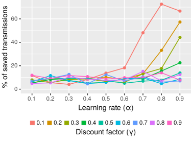
Figure 1: Impact of the Q-Learning agent in the reduction of the number of transmissions.

In our experiments, the number of transmissions in a sensor node achieves its maximum when the sampling interval is $30$ seconds and its minimum when the sampling interval is $240$ seconds. Intuitively, setting the sampling interval to $60$, $120$ and $240$ seconds represents a reduction of respectively $50\%$, $75\%$ and $87.5\%$ in the maximum number of transmissions.

Figure 1 illustrates how many transmissions could be saved when the Q-Learning was adopted to adjust the sensor node’s sampling interval. In this plot, we consider that the Q-Learning agent triggers one new transmission every time a new sampling interval is set. In the best case, the number of transmissions can be reduced to up to $72.57\%$ of its maximum, when $\alpha=0.8$ and $\gamma=0.1$. As observed in our preliminary results, the highest savings happen when $\alpha$ is high (i.e., $\alpha\in\{0.7,0.8,0.9\}$) and $\gamma$ is low (i.e., $\gamma\in\{0.1,0.2,0.3\}$). That is, when the agent learns mostly from recent environment feedback and minimally from the expected reward. We highlight the importance of setting proper values to $\alpha$ and $\gamma$, given that most of the cases do not reduce by more than $15\%$ the maximum number of transmissions.

VI-B Efficiency

Figure 2 shows the percentage of consecutive measurements that differ by more than $\tau$. To help the understanding of the magnitude of the errors, we added four baselines that represent the rates that would be observed if the sampling intervals were fixed, based on the same data used in the simulations. Again, the best results happen in scenarios using higher $\alpha$ (i.e., $\alpha\in\{0.7,0.8,0.9\}$) and lower $\gamma$ (i.e., $\gamma\in\{0.1,0.2,0.3\}$).

In the best result ($\alpha=0.9$ and $\gamma=0.1$), the rate of measurements over $\tau$ is similar to the scenario with a fixed sampling interval of $30$ seconds. With the sampling interval set to $30$ seconds, we observed $16509$ pairs of consecutive measurements that differed by more than $\tau$ with an average of $0.063^{\text{o}}$C. Using Q-Learning, we observed $13679$ pairs of consecutive measurements that differed by more than $\tau$, which differed by $0.078^{\text{o}}$C on average.

These small values strengthen the relevance of the reduction in the number of transmissions shown above, because they indicate that the avoided transmissions are, in fact, worthless in this scenario. In conclusion, a real application that adopted Q-Learning with $\alpha=0.9$ and $\gamma=0.1$ would have saved around $65\%$ of its transmissions and observed an average of $0.024^{\text{o}}$C in the absolute difference between two consecutive measurements.

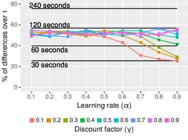
Figure 2: Percentage of consecutive measurements that differ by more than $\tau$. The black lines show the percentage observed the sampling intervals fixed to the values written in the plot.

VII Conclusion

In this work, we adopted a Reinforcement Learning (RL) technique called Q-Learning to adjust the sampling interval of sensor nodes according to the expected changes in the environment. After explaining how the adaptive sampling can be formulated as a machine learning problem and showing that the environment’s evolution can impact our algorithm, we evaluated the reduction in the number of transmissions and the quality of the reported data. We presented the steps to setup the algorithm (i.e., states, actions, and reward) in a way that can be further exploited in several scenarios.

In our simulations, we could avoid nearly $73\%$ of transmissions in the best combination of parameters for the Q-Learning algorithm. Observing the quality of the reported data, we noticed that the proposed mechanism keeps similar quality to what would be observed if the smallest sampling interval was adopted. Assuming that the radio transmissions are the main cause of energy consumption in monitoring WSNs, this solution may lead to significant savings in any scenario with wireless sensor nodes. Furthermore, the reduction in the number of transmissions can support WSNs to admit more sensor nodes, increasing their range and generating more knowledge about the monitored area. To optimize resource usage, this mechanism can be further combined with other approaches, such as data aggregation and data compression.

We conclude that the use of an RL algorithm to control sensor nodes’ sampling intervals can be very profitable. Furthermore, we highlight that the proper choice of its parameters ($\alpha$ and $\gamma$) can significantly impact the results. For instance, in our experiments, higher values of $\alpha$ (i.e., $\alpha\in\{0.8,0.9\}$) and lower values of $\gamma$ (i.e., $\gamma\in\{0.1,0.2\}$) provided the best cost-benefit in the “saved transmissions”-“high quality” relationship. In our future work, we plan to implement the mechanism presented here to control the sampling interval of wireless sensor nodes in a real deployment.

References

- [1] R. S. Sutton and A. G. Barto, Introduction to Reinforcement Learning, 1st ed. Cambridge, MA, USA: MIT Press, 1998.
- [2] M. Nurchis, R. Bruno, M. Conti, and L. Lenzini, “A self-adaptive routing paradigm for wireless mesh networks based on reinforcement learning,” in Proceedings of the 14th ACM international conference on Modeling, analysis and simulation of wireless and mobile systems. ACM, 2011, pp. 197–204.
- [3] S. Li, X. Kong, and D. Lowe, “Dynamic path determination of mobile beacons employing reinforcement learning for wireless sensor localization,” in Advanced Information Networking and Applications Workshops (WAINA), 2012 26th International Conference on. IEEE, 2012, pp. 760–765.
- [4] M. Mihaylov, K. Tuyls, and A. Nowé, Adaptive and Learning Agents: Second Workshop, ALA 2009, Held as Part of the AAMAS 2009 Conference in Budapest, Hungary, May 12, 2009. Revised Selected Papers. Berlin, Heidelberg: Springer Berlin Heidelberg, 2010, ch. Decentralized Learning in Wireless Sensor Networks, pp. 60–73.
- [5] Y.-A. Le Borgne, S. Santini, and G. Bontempi, “Adaptive model selection for time series prediction in wireless sensor networks,” Signal Processing, vol. 87, no. 12, pp. 3010–3020, Dec. 2007.
- [6] H. Malik, A. S. Malik, and C. K. Roy, “A methodology to optimize query in wireless sensor networks using historical data,” Journal of Ambient Intelligence and Humanized Computing, vol. 2, pp. 227–238, Jun. 2011.
- [7] G. M. Dias, T. Adame, B. Bellalta, and S. Oechsner, “A self-managed architecture for sensor networks based on real time data analysis,” to appear in Future Technologies Conference 2016. IEEE, Dec. 2016. [Online]. Available: http://arxiv.org/abs/1605.09011
- [8] S. Madden, “Intel lab data,” http://db.lcs.mit.edu/labdata/labdata.html, Jun. 2004.
- [9] L. Breiman, “Random forests,” Machine learning, pp. 1–33, 2001.