Quasi-periodic oscillations in superfluid, relativistic magnetars with nuclear pasta phases

Abstract

We study the torsional magneto-elastic oscillations of relativistic superfluid magnetars and explore the effects of a phase transition in the crust-core interface (nuclear pasta) which results in a weaker elastic response. Exploring various models with different extension of nuclear pasta phases, we find that the differences in the oscillation spectrum present in purely elastic modes (weak magnetic field), are smeared out with increasing strength of the magnetic field. For magnetar conditions, the main characteristic and features of models without nuclear pasta are preserved. We find in general two classes of magneto-elastic oscillations which exhibit a different oscillation pattern. For $B_{p}<4\times 10^{14}$G, the spectrum is characterised by the turning points and edges of the continuum which are mostly confined into the star’s core, and have no constant phase. Increasing the magnetic field, we find, in addition, several magneto-elastic oscillations which reach the surface and have an angular structure similar to crustal modes. These global magneto-elastic oscillations show a constant phase and become dominant when $B_{p}>5\times 10^{14}$G. We do not find any evidence of fundamental pure crustal modes in the low frequency range (below 200 Hz) for $B_{p}\geq 10^{14}$G.

1 Introduction

The first data set for applying Astereoseismology in neutron stars was provided by magnetars. The strong magnetic field of these stars, $B>10^{14}$G, powers a rich X-ray activity of persistent and sporadic emission (Mereghetti, 2008). The most energetic events are the giant flares which can radiate up to $10^{46}$ erg per second. In the tail of the three giant flares so far observed (SGR 0526-66, SGR 1900+14, SGR 1806-20), a series of Quasi Periodic Oscillations (QPOs) with different duration and frequency was revealed by spectral analyses (Israel et al., 2005; Strohmayer & Watts, 2005; Watts & Strohmayer, 2006). The majority of them reside in the low frequency band $18~{}\textrm{Hz}<\nu<200$ Hz, but oscillations have also been observed in the SGR 1806-20 at $625$ Hz and $1840$ Hz. Recently, the analysis of the storm events in magnetars have revealed a few QPOs also in intermediate flares (Huppenkothen et al., 2014a, b), which occur more frequently than giant flares but are less energetic.

Since their detection, it was immediately clear that QPOs could originate from star oscillations and therefore used to explore the properties of magnetar physics. Initially, they were identified with crustal shear modes (Duncan, 1998; Israel et al., 2005), but it was soon pointed out that the strong magnetic field of magnetars might dominate the global oscillations and significantly influence the vibrations of the crust (Levin, 2006; Glampedakis et al., 2006; Levin, 2007). In particular, torsional magnetic oscillations of a purely poloidal magnetic field can produce bands of continuum spectrum, which can rapidly absorb the crustal modes that reside within them (van Hoven & Levin, 2011, 2012). In this theoretical model, the spectrum is characterised by magnetically dominated modes, the turning points and edges of the continuum bands, and the crustal modes whose frequency lies within the continuum gaps. In particular, the interpretation of the $625$ Hz QPO as a torsional shear overtone appeared difficult. At this high frequency the continuum bands should overlap and therefore quickly damp this mode. Recently Huppenkothen, Watts & Levin (2014) have re-analysed this QPO in the data and found that it can be consistent with either a long-lived or an intermittent oscillation with decaying time $\sim 0.5s$. In the latter case, the QPO must be re-excited during the giant flare many times from a process at moment unknown. The continuum spectrum may be however an artefact of oversimplified theoretical models, which consider magneto-elastic torsional oscillations in a purely poloidal magnetic field. Indeed, the continuum could be reduced or destroyed by the interaction between the torsional and poloidal modes via mixed poloidal-toroidal magnetic field configurations (Colaiuda & Kokkotas, 2012) or by tangled magnetic fields (van Hoven & Levin, 2011; Link & van Eysden, 2015; Sotani, 2015).

Several works have studied the oscillations of magnetised neutron stars with various degrees of model sophistication. With plane wave approximation (van Hoven & Levin, 2008; Andersson et al., 2009), in time domain simulations (Sotani et al., 2007, 2008; Colaiuda et al., 2009; Gabler et al., 2011; van Hoven & Levin, 2011, 2012; Gabler et al., 2012; Gabler et al., 2013) and as eigenvalue problems (Lee, 2008; Asai & Lee, 2014; Asai et al., 2015, 2016). In particular, Colaiuda & Kokkotas (2011) were able to identify the QPOs with a set of magnetic and crustal modes and a specific Equation of State (EoS) without superfluid matter.

Mature neutron stars are however expected to contain superfluid and superconducting constituents, which may strongly influence the dynamics and the oscillation spectrum. The effects of superfluidity on the crustal modes have been studied by many authors (Samuelsson & Andersson, 2009; Passamonti & Andersson, 2012; Sotani et al., 2013), while the effects on the non-axisymmetric magnetic oscillations were addressed by Passamonti & Lander (2013). In superfluid magnetars, the torsional magneto-elastic waves were recently studied in relativistic (Gabler et al., 2013, 2016) and in Newtonian stars (Passamonti & Lander, 2014), which show a richer spectrum in superfluid models. Besides the magneto-elastic oscillations found in non-superfluid stars, there are several waves which have an angular structure similar to crustal oscillations. These waves are however present both in the core and the crust and may have discrete character (Gabler et al., 2013, 2016).

Another important aspect for the QPO interpretation is the wave transmission from the star to the external magnetosphere. In the standard magnetar model, it is believed that the star’s vibrations can modulate the X-ray emission of a fireball anchored in the magnetosphere near the star surface and thus produce the observed QPOs. Progresses in this direction were recently made by Link (2014) with a plane-wave analysis and by Gabler et al. (2014) with more elaborated models, which couple the internal wave dynamics with the magnetosphere oscillations.

In this work, we study the torsional magneto-elastic oscillations of magnetars. In our model, we consider the effects of entrainment as well as that of nuclear pasta phase on the oscillation spectrum. This new phase can be present as a transition region between the bottom of the crust and the core (e.g. see Schneider et al., 2013; Caplan et al., 2015, and references therein), where nuclei can assume exotic shapes, like rods, plates, bubbles, etc. The elasticity of this part of the crust can be quite different from regular cubic lattices of ions (Pethick & Potekhin, 1998), and its effects on the crustal modes quite relevant (Sotani, 2011; Gearheart et al., 2011). These works have shown, in fact, that the crustal modes have lower frequencies and a denser spectrum when the pasta phase region is wider. The possible identification of these modes with the QPOs can therefore provide interesting results to understand the physics of the crust. However, Sotani (2011) and Gearheart et al. (2011) focus on the crustal modes and neglect the magnetic field, which, as described before, can significantly modify the results. In this work, we try to clarify this issue and see whether the presence of nuclear pasta phases changes the spectrum of the torsional magneto-elastic waves.

We present the formalism and the properties of our magnetar model in Secs. 2 and 3. The perturbation equations to study the magneto-elastic torsional oscillations are given in Sec. 4 and in the Appendix, while the numerical framework is described in Sec. 5. The results are presented in Sec. 6 and the conclusions can be found in Sec. 7.

2 Formalism

During the cooling of a neutron star, when the temperature drops below the superfluid critical temperature, $T_{c}\simeq 10^{9}$K, the neutrons of the core and the inner crust and the protons of the core can become, respectively, superfluid and superconducting. As a result, the neutron interaction with the other particles is weaker and completely different from the non-superfluid state. On the other hand, protons and electrons in the core are so strongly coupled by electromagnetic interaction that they can be considered as a single comoving neutral fluid. The dynamics is then naturally described by two degrees of freedom, a gas of free superfluid neutrons and a neutral mixture of charged particles, which for simplicity we will call “protons”. In the inner crust, the second degree of freedom is given by the heavy nuclei of the lattice. To discern the various components we use Roman letter x, y, …as constituent index. Specifically, we denote with the letter $\mathrm{n}$ and $\mathrm{p}$ the superfluid neutrons and the neutral mixture of the core, and with $\mathrm{f}$ and $\mathrm{c}$ the free superfluid neutrons and the nuclei of the inner crust. These matter indices are not summed over when repeated. We assume in this work a strong superfluid regime, i.e. the star’s temperature is well below the neutron critical temperature $T_{\mathrm{c}\mathrm{n}}$.

In general, superfluid gap models suggest that protons become superconducting at $T\approx 5\times 10^{9}$K, when neutrons might be still in a normal state. The proton superfluid transition modifies significantly the properties of the magnetic field, which now likely reconfigures itself in an array of fluxtubes (Type II superconductivity). Although very interesting, we neglect in this work the effects of superconductivity on the oscillation modes. However, it is not still clear if the magnetic field in magnetars exceeds the critical value ($10^{15}\textrm{G}-10^{16}$G), above which Type II superconductivity is destroyed. Another possibility is that the superconducting states could be limited to a shell near the crust/core interface (Sinha & Sedrakian, 2014).

We study the dynamics of this system with the relativistic two-fluid model, based on the constrained variational approach developed by Carter and collaborators (Carter, 1989; Carter & Langlois, 1998; Carter & Samuelsson, 2006). The fundamental quantities of the constrained variational formalism are the master function $\Lambda$ and the particle currents. The particle fluxes are defined by the following expression:

$$n_{\mathrm{x}}^{\alpha}\equiv n_{\mathrm{x}}u^{\alpha}_{\mathrm{x}}\,,$$ (1)

where $u^{\alpha}_{\mathrm{x}}$ is the velocity of the x fluid, and $n_{\mathrm{x}}$ is the particle density. It is determined by the normalization condition, $n_{\mathrm{x}}^{2}=-n_{\mathrm{x}}^{\alpha}n_{\alpha}^{\mathrm{x}}$. The master function of a fluid star is in general a function of the scalars which can be built from the number density currents, i.e. $n_{\mathrm{x}}^{2}$ and $n_{\mathrm{x}\mathrm{y}}^{2}=-n_{\mathrm{x}}^{\alpha}n_{\alpha}^{\mathrm{y}}$. The conjugate momenta arise naturally, in the variational approach, from the definition

$$\mu_{\alpha}^{\mathrm{x}}=\left(\frac{\partial\Lambda}{\partial n_{\mathrm{x}}^{\alpha}}\right)_{n_{\mathrm{y}}^{\alpha}}\,.$$ (2)

For superfluid relativistic stars with crust and magnetic field, the master function as well as the derivation of the dynamical equations have been described in detail by Carter & Samuelsson (2006) (see also Samuelsson & Andersson, 2009, for an application to non-magnetised stars). We do not provide here all the details of the formalism but consider only the essential parts (see Andersson & Comer, 2007, for a review).

The dynamical equations are given by the particle number conservation equations:

$$\nabla_{\alpha}n_{\mathrm{x}}^{\alpha}=0\,,$$ (3)

and by the momentum equations:

$$2n_{\mathrm{f}}^{\alpha}\nabla_{\left[\alpha\right.}\mu^{\mathrm{f}}_{\left.\beta\right]}=0\,,$$ (4)

$$2n_{\mathrm{c}}^{\alpha}\nabla_{\left[\alpha\right.}\mu^{\mathrm{c}}_{\left.\beta\right]}=f_{\beta}^{\mathrm{c}}\,,$$ (5)

where $f_{\beta}^{\mathrm{c}}$ is the force density acting on the mixture of charged particles $\mathrm{c}$. The same equations are valid for the core, provided the indices $\mathrm{f}$ and $\mathrm{c}$ are, respectively, replaced with $\mathrm{n}$ and $\mathrm{p}$. The force density in the crust reads

$$f_{\beta}^{\mathrm{c}}=-\nabla_{\alpha}\left(\pi^{\alpha}_{\beta}+M^{\alpha}_{\beta}\right)\,,$$ (6)

where $\pi^{\alpha\beta}$ is the stress-energy tensor of the solid crust, while $M^{\alpha\beta}$ is the magnetic stress energy tensor. In the core, the “proton” fluid feels only the magnetic force:

$$f_{\beta}^{\mathrm{p}}=-\nabla_{\alpha}M^{\alpha}_{\beta}\,.$$ (7)

In ideal MHD, the magnetic energy-momentum tensor is given by

$$M^{\alpha\beta}=\frac{1}{4\pi}\left(B^{2}u^{\alpha}_{\mathrm{x}}u^{\beta}_{\mathrm{x}}+\frac{B^{2}}{2}g^{\alpha\beta}-B^{\alpha}B^{\beta}\right)\,,$$ (8)

where $\mathrm{x}=\mathrm{p}$ in the core and $\mathrm{x}=\mathrm{c}$ in the crust.

The stress energy tensor for an isotropic crust can be derived with the formalism introduced by Carter & Quintana (1972) (see also Karlovini & Samuelsson, 2003, for more general cases). The first step is to define the stress energy tensor in terms of the shear modulus $\check{\mu}$ and the shear tensor $\Sigma^{\alpha\beta}$:

$$\pi^{\alpha\beta}=-2\check{\mu}\Sigma^{\alpha\beta}\,.$$ (9)

Secondly, the shear tensor is defined by the following equation:

$$\mathcal{L}_{u}\Sigma^{\alpha\beta}=\sigma^{\alpha\beta}\,,$$ (10)

where $\mathcal{L}_{u}$ is the Lie derivative with respect to $u^{\alpha}$. The stress tensor is

$$\sigma^{\alpha\beta}=\frac{1}{2}\left(u^{\alpha}_{\mathrm{c};\nu}\bot^{\nu\beta}+u^{\beta}_{\mathrm{c};\nu}\bot^{\nu\alpha}\right)-\frac{1}{3}\bot^{\alpha\beta}u^{\nu}_{\mathrm{c};\nu}\,,$$ (11)

and the projector tensor, $\bot^{\alpha\beta}$, is defined as follows

$$\bot^{\alpha\beta}=g^{\alpha\beta}+u_{\mathrm{c}}^{\alpha}u_{\mathrm{c}}^{\beta}\,.$$ (12)

To close the system of equations (3)-(5) we need an evolution equation for the magnetic field, which is given by the relativistic induction equation. In ideal MHD it reads

$$\nabla_{\alpha}\left(u_{\mathrm{c}}^{\alpha}B^{\beta}+u_{\mathrm{c}}^{\beta}B^{\alpha}\right)=0\,.$$ (13)

The usual replacement of $u_{\mathrm{c}}^{\alpha}$ with $u_{\mathrm{p}}^{\alpha}$ must be done in the core.

3 Neutron star model

In this section, we describe the properties of our neutron star model, which represents a relativistic superfluid magnetar with a poloidal magnetic field and a realistic equation of state. The strong magnetic field and the slow rotation of magnetars have a negligible effect on the global structure of the star. These stars are therefore well described by a spherically symmetric spacetime. Considering a star with an unstrained crust, the spacetime is given by the following line element:

$$ds^{2}=-e^{2\nu}dt^{2}+e^{2\lambda}dr^{2}+r^{2}d\theta^{2}+r^{2}\sin\theta^{2}d\phi^{2}\,,$$ (14)

where $\nu$ and $\lambda$ are functions only of the radial coordinate. They are determined by solving the Tolman-Oppenheimer-Volkoff equations with a specific EoS. The background 4-velocity and the conjugate momenta, respectively, read

$$u^{\alpha}=\left(e^{-\nu},\vec{0}\right)\,,\qquad\mu^{\mathrm{x}}_{\alpha}=\left(-\mu^{\mathrm{x}}e^{\nu},\vec{0}\right)\,,$$ (15)

where $\mu^{\mathrm{x}}$ is the chemical potential of the x fluid.

3.1 Equation of State

We use the Douchin-Haensel EoS, which describes the state of matter both in the core and the crust of a neutron star  (Douchin & Haensel, 2001). It is based on a Skyrme-type energy density functional (SLy model). Our baseline neutron star model has $M=1.4M_{\odot}$ and $R=11.66$ km, while the crust-core transition appears at density $\rho_{cc}=1.285\times 10^{14}\textrm{g cm}^{-3}$, which corresponds to a radial position $R_{cc}=10.79$ km. It is important to notice that the entrainment properties illustrated in Sec. 3.4 have not been derived for the DH EoS. Similar concerns apply to the pasta phases which are not present in this EoS (Douchin & Haensel, 2000). We use the DH EoS because it provides all necessary inputs to model our superfluid neutron star and to facilitate the comparison with previous works. In any case, the qualitative nature of our results should not change dramatically with other EoSs which we plan to explore in future work (see for instance Fantina et al., 2012; Potekhin et al., 2013; Sharma et al., 2015).

3.2 Background magnetic field

The magnetic field in our model has a poloidal geometry and it is determined by solving the Grad-Shafranov equation. In a multi-fluid system, the electric currents can be quite different from a single fluid case. For instance the superfluid neutrons do not contribute to the inertia and in the crust only the free electrons can be able to produce electric currents. To simplify our approach we neglect the effect of multi-fluid physics on the background magnetic field configuration. We therefore solve the Grad-Shafranov as in a single fluid star and avoid unnecessary complexity at this point. In fact, the uncertainty introduced by this assumption is smaller than other approximations made in this kind of studies. For instance, it is well known that purely poloidal fields are unstable and cannot be the final magnetic field configuration in a mature neutron star. Furthermore, by adopting a single fluid magnetic field solution we can much easily compare our results with the literature.

In the coordinate basis, the magnetic field components of a dipolar field can be defined as follows

$$B^{r}=\mathrm{e}^{-\lambda}\frac{2\cos\theta}{r^{2}}a_{1}\,,\qquad B^{\theta}=-{\mathrm{e}^{-\lambda}}\frac{\sin\theta}{r^{2}}\frac{da_{1}}{dr}\,,$$ (16)

where $a_{1}(r)$ is a solution of the Grad-Shafranov equation:

$$\frac{d^{2}a_{1}}{dr^{2}}+\frac{d}{dr}\left(\nu-\lambda\right)\frac{da_{1}}{dr}-\frac{2}{r^{2}}\mathrm{e}^{2\lambda}a_{1}=-4\mathrm{\pi}c_{0}r^{2}\left(\varepsilon+p\right)\mathrm{e}^{2\lambda}\,.$$ (17)

The quantities $\varepsilon$ and $p$ are, respectively, the mass-energy and the pressure, while $c_{0}$ is a constant. To solve equation (17) we must specify the boundary conditions at both the origin and the surface. Regularity of the solution at the origin requires $a_{1}=\alpha_{0}r^{2}$ (when $r\to 0$), where $\alpha_{0}$ is a constant. At the surface, the solution must be matched with an external magnetic field, which we consider a dipolar field in the vacuum. The condition at the surface is therefore:

$$a_{1}=-\frac{3\mu_{0}}{8M^{3}}r^{2}\left[\ln\left(1-\frac{2M}{r}\right)+\frac{2M}{r}+\frac{2M^{2}}{r^{2}}\right]\,,$$ (18)

where $M$ is the star’s mass and $\mu_{0}$ the magnetic dipole moment in geometric units. The two constants $\alpha_{0}$ and $c_{0}$ can be determined from the numerical integration in order to satisfy the boundary conditions. The solution is determined up to the arbitrary multiplicative factor $\mu_{0}$, which is fixed by the value of the poloidal magnetic field at the magnetic pole $B_{p}$. In our model, the average magnetic field of the star is roughly $\langle B\rangle\simeq 1.45B_{p}$.

3.3 Shear modulus

For the shear modulus in the crust we use the low temperature limit of the formula derived by Strohmayer et al. (1991):

$$\check{\mu}=0.1194\left(\frac{4\pi}{3}\right)^{1/3}n_{i}^{4/3}\left(Ze\right)^{2}\,,$$ (19)

where $n_{i}$ is the ion number density and $Ze$ the ion charge. Equation (19) assumes a body-centered-cubic crystalline lattice, while at the bottom layers of the crust there might be, in some EoS, stable configurations of “pasta phases”. In these regions, the strong and Coulomb interaction can modify the shape of the nuclei, which can adopt non-spherical shapes. These exotic phases can appear when the density is $\rho_{0}\lesssim\rho\lesssim 0.1\rho_{0}$, where $\rho_{0}=2.7\times 10^{14}~{}\textrm{g cm}^{-3}$ is the nuclear saturation density (Schneider et al., 2013). It is worth noticing that if the various shapes which form the nuclear pasta have regular structures, the shear modulus may be anisotropic. However, if these structures are disordered, on average, the anisotropy degree can be partially reduced (Schneider et al., 2013; Horowitz et al., 2015).

The elastic reaction of this exotic phases is still unknown, even if some preliminary work is present in the literature (see Chamel & Haensel, 2008, for a review), but in any case the rigidity of the crust is expected to decrease. To model the shear modulus between a “normal” solid crust, which is described by equation (19), and the core, where $\check{\mu}=0$, we use a function which smoothly joins these to regions given by

$$\check{\mu}=c_{1}\left(\rho-\rho_{cc}\right)\left(\rho-c_{2}\right)\,,$$ (20)

where $\rho_{cc}$ is the density at the crust/core interface, and $c_{1}$ and $c_{2}$ are two interpolation constants. Eq. 20 describes the shear modulus in the density range $\rho_{ph}\leq\rho\leq\rho_{cc}$ where $\rho_{ph}$ is the pasta phase transition density. In this work we consider this transition in the range $10^{13}\textrm{g cm}^{-3}\lesssim\rho_{ph}\lesssim 10^{14}\textrm{g cm}^{-3}$ (see Fig. 1).

The only difference between Eq. 20 and the expression used by Sotani (2011) is in the term given by the first bracket, which was originally squared, i.e. $\left(\rho-\rho_{cc}\right)^{2}$. We have first tried the same expression, but we found some problems of convergence for the eigenfrequencies of the shear mode overtones. This problem is removed by using equation (20), which goes linearly to zero when $\rho$ gets close to $\rho_{cc}$ (see Fig. 1).

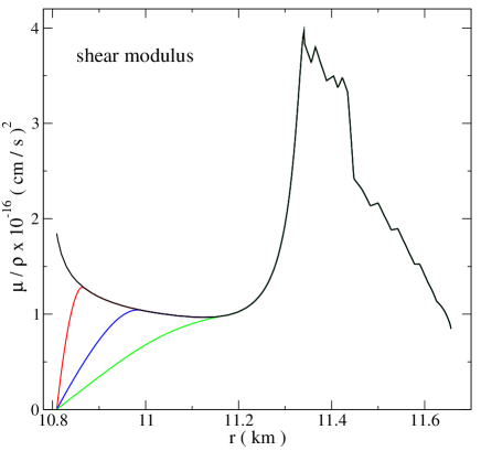
Figure 1: Shear modulus ($\mu/\rho$) of our stellar model with different pasta phase transition density $\rho_{ph}$ . The black line describe a star without pasta phase, while the other three curves show model with decreasing $\rho_{ph}$. More precisely, the red line corresponds to $\rho_{ph}=10^{14}$ g cm^-3, the blue line to $\rho_{ph}=5\times 10^{13}$ g cm^-3 and the green lines represent the $\rho_{ph}=10^{13}$ g cm^-3 case.

3.4 Entrainment

In superfluid stars the interaction between the various particle species changes with respect to normal dissipative processes. Superfluid neutrons and protons can interact via the mutual friction which is a dissipative processes mediated by superfluid vortices, which depends on the star’s rotation rate. Magnetars are slowly rotating stars, thus this effect is likely negligible in the magneto-elastic oscillations. There is also another non-dissipative process, called entrainment, that couples the dynamics of various constituents of a superfluid system. The entrainment in the core of a neutron star is driven by the strong interaction force between the nucleons and is typically weak. In the inner crust, superfluid neutrons interact with the nuclei lattice via Bragg scattering and the entrainment can be quite strong (see Chamel, 2012, and reference therein). A result of entrainment is that, in a superfluid, the constituent momentum is not aligned with the velocity, but contains also a contribution of the other particle specie. Normally, the entrainment is described by a quantity $\varepsilon_{\mathrm{x}}$ which is strictly related to the effective mass, $m_{\mathrm{x}}^{\star}$, through the following relation:

$$\varepsilon_{\mathrm{x}}=1-\frac{m_{\mathrm{x}}^{\star}}{m_{\mathrm{x}}}\,.$$ (21)

In our model, we consider the entrainment profile provided in Chamel (2008) for the core, and Chamel (2005, 2006, 2012) for the crust. In practise, we use the same mathematical structure described in Passamonti & Lander (2014), but applied to a tabulated EoS. The maximum effect of the entrainment is expected in the inner crust where the effective mass of neutrons can be as large as $m_{\mathrm{f}}^{\star}\simeq 14m_{\mathrm{f}}$.

4 Perturbation Equations

In this section, we summarize the perturbation equations used to study axisymmetric axial (torsional) oscillations of relativistic superfluid magnetars. We use the Cowling approximation, i.e. we neglect the perturbations of the space-time. It provides accurate results for the crustal and Alfvén torsional modes.

In a non-rotating axisymmetric star, the torsional modes satisfy the number conservation equation by definition, $\nabla_{\alpha}\delta n_{\mathrm{x}}^{\alpha}=0$. The perturbed momentum conservation equations (4)-(5) read

$$2\delta\left(n_{\mathrm{f}}^{\alpha}\nabla_{\left[\alpha\right.}\mu^{\mathrm{f}}_{\left.\beta\right]}\right)=0\,,$$ (22)

$$2\delta\left(n_{\mathrm{c}}^{\alpha}\nabla_{\left[\alpha\right.}\mu^{\mathrm{c}}_{\left.\beta\right]}\right)=\delta f_{\beta}^{\mathrm{c}}\,,$$ (23)

which, using the symmetry of the problem, leads to the following equations:

$$\partial_{t}\delta\mu_{\phi}^{\mathrm{f}}=0\,,$$ (24)

$$n_{\mathrm{c}}\,\mathrm{e}^{-\nu}\,\partial_{t}\delta\mu^{\mathrm{c}}_{\phi}=\delta f_{\phi}^{\mathrm{c}}\,.$$ (25)

Here, we have used the indices $\mathrm{c}$ and $\mathrm{f}$ for the crust constituents, but equations (24)-(25) are formally valid also for the core. The conjugate momenta are related to the velocity perturbations as follows:

$$\delta\mu^{\mathrm{f}}_{\phi}=\mathcal{K}_{\mathrm{f}\mathrm{f}}n_{\mathrm{f}}\,\delta u^{\mathrm{f}}_{\phi}+\mathcal{K}_{\mathrm{f}\mathrm{c}}n_{\mathrm{c}}\,\delta u^{\mathrm{c}}_{\phi}\,,$$ (26)

$$\delta\mu^{\mathrm{c}}_{\phi}=\mathcal{K}_{\mathrm{c}\mathrm{f}}n_{\mathrm{f}}\,\delta u^{\mathrm{f}}_{\phi}+\mathcal{K}_{\mathrm{c}\mathrm{c}}n_{\mathrm{c}}\,\delta u^{\mathrm{c}}_{\phi}\,,$$ (27)

where we have used the components of the entrainment matrix:

$$\mathcal{K}_{\mathrm{f}\mathrm{f}}=-2\frac{\partial\Lambda}{\partial n_{\mathrm{f}}^{2}}\,,$$ (28)

$$\mathcal{K}_{\mathrm{c}\mathrm{c}}=-2\frac{\partial\Lambda}{\partial n_{\mathrm{c}}^{2}}\,,$$ (29)

$$\mathcal{K}_{\mathrm{f}\mathrm{c}}=\mathcal{K}_{\mathrm{c}\mathrm{f}}=-\frac{\partial\Lambda}{\partial n_{\mathrm{c}\mathrm{f}}^{2}}\,.$$ (30)

Up to second order corrections in the relative velocity between the $\mathrm{c}$ and $\mathrm{f}$ fluids, the entrainment matrix is given by (Samuelsson & Andersson, 2009):

$$\mathcal{K}_{\mathrm{f}\mathrm{f}}=\frac{1}{nn_{\mathrm{f}}}\left[\left(\varepsilon+p\right)-\rho\epsilon_{\mathrm{f}}\right]\,,$$ (31)

$$\mathcal{K}_{\mathrm{c}\mathrm{c}}=\frac{1}{nn_{\mathrm{c}}}\left[\left(\varepsilon+p\right)-\frac{n_{\mathrm{f}}}{n_{\mathrm{c}}}\rho\epsilon_{\mathrm{f}}\right]\,,$$ (32)

$$\mathcal{K}_{\mathrm{f}\mathrm{c}}=\mathcal{K}_{\mathrm{c}\mathrm{f}}=\frac{\rho\epsilon_{\mathrm{f}}}{nn_{\mathrm{c}}}\,,$$ (33)

where $n=n_{\mathrm{c}}+n_{\mathrm{f}}$. The entrainment parameter $\varepsilon_{\mathrm{f}}$ is related to the effective mass of the free neutrons and has been defined in equation (21).

The torsional oscillations in a spherical star with magnetic field can be studied with a single wave-like equation for the conglomerate of charged components. From equation (24) we can write

$$\partial_{t}\delta u^{\mathrm{f}}_{\phi}=-\frac{\mathcal{K}_{\mathrm{f}\mathrm{c}}}{\mathcal{K}_{\mathrm{f}\mathrm{f}}}\frac{n_{\mathrm{c}}}{n_{\mathrm{f}}}\,\partial_{t}\delta u^{\mathrm{c}}_{\phi}\,,$$ (34)

which inserted in equation (25) provides

$$\chi\left(\varepsilon+p\right)e^{-2\nu}\,\frac{\partial^{2}\xi_{\phi}^{\mathrm{c}}}{\partial t^{2}}=\delta f_{\phi}^{\mathrm{c}}\,.$$ (35)

Here, we have defined the Lagrangian displacement $\xi_{\mathrm{c}}^{\alpha}$ for the $\mathrm{c}$ fluid:

$$\delta u_{\mathrm{c}}^{\alpha}=\mathcal{L}_{u}\xi_{\mathrm{c}}^{\alpha}=\mathrm{e}^{-\nu}\xi_{\mathrm{c}}^{\alpha}\,,$$ (36)

and a quantity that accounts for the entrainment (Samuelsson & Andersson, 2009):

$$\chi=\frac{x_{\mathrm{c}}\left(\varepsilon+p\right)-\rho\epsilon_{\mathrm{f}}}{\varepsilon+p-\rho\epsilon_{\mathrm{f}}}=1-x_{\mathrm{f}}\frac{\varepsilon+p}{\varepsilon+p-\rho\epsilon_{\mathrm{f}}}\,,$$ (37)

where $x_{\mathrm{c}}=n_{\mathrm{c}}/n$ and $x_{\mathrm{f}}=n_{\mathrm{f}}/n$. For a zero entrainment system, $\varepsilon_{\mathrm{f}}=0$, and $\chi=x_{\mathrm{c}}$. Note that in the Newtonian limit, $\chi$ tends to $x_{\mathrm{c}}\,\varepsilon_{\star}^{-1}$ which is the entrainment parameter used in Passamonti & Lander (2014).

In the crust the linearised force reads:

$$\delta f_{\phi}^{\mathrm{c}}=-\nabla_{\alpha}\delta\pi_{\,\,\phi}^{\alpha}-\nabla_{\alpha}\delta M_{\,\,\phi}^{\alpha}\,,$$ (38)

while in the core only the magnetic force is present,

$$\delta f_{\phi}^{\mathrm{p}}=-\nabla_{\alpha}\delta M_{\,\,\phi}^{\alpha}\,.$$ (39)

The equations for the perturbation of the magnetic stress-energy tensor have been already presented in several works (see for instance Sotani et al., 2007). In particular, the perturbation of the magnetic field $\delta B^{\alpha}$, can be expressed in terms of the Lagrangian displacement $\xi^{\alpha}$ by using the linearised induction equation

$$\delta\left[\nabla_{\alpha}\left(u^{\alpha}_{\mathrm{c}}B^{\beta}+u^{\beta}_{\mathrm{c}}B^{\alpha}\right)\right]=0\,.$$ (40)

Without repeating the same calculations we directly provide the final linearised equation, written in the coordinate basis, to study axisymmetric torsional oscillations in a magnetised superfluid star with crust:

$$\left[\chi\left(\varepsilon+p\right)+\frac{B^{2}}{4\pi}\right]\textrm{e}^{-2\nu}\frac{\partial^{2}\xi_{\mathrm{c}}^{\phi}}{\partial t^{2}} =A_{1}\frac{\partial^{2}\xi_{\mathrm{c}}^{\phi}}{\partial r^{2}}+A_{2}\frac{\partial^{2}\xi_{\mathrm{c}}^{\phi}}{\partial\theta^{2}}+A_{3}\frac{\partial^{2}\xi_{\mathrm{c}}^{\phi}}{\partial r\partial\theta}$$

$$+A_{4}\frac{\partial\xi_{\mathrm{c}}^{\phi}}{\partial r}+A_{5}\frac{\partial\xi_{\mathrm{c}}^{\phi}}{\partial\theta}\,.$$ (41)

The coefficients $A_{k}$ depends on the background variables and are given in the Appendix A. The core’s protons obey the same wave equation with the coefficients $A_{k}$ taken in the zero shear modulus limit, $\check{\mu}=0$.

4.1 Boundary conditions

The symmetry of the problem allows us to study the time evolution of equation (41) in the 2D-region $0\leq r\leq R$ and $0\leq\theta\leq{\rm\pi}/2$. At the boundary of this domain we must obviously impose appropriate conditions.

The regularity of the perturbation equation at the origin requires that $\xi^{\phi}_{\mathrm{p}}=0$ at $r=0$. At the magnetic axis, $\theta=0$, the Lagrangian displacement must satisfy, in the coordinate basis, the following relation $\partial_{\theta}\xi^{\phi}_{\mathrm{x}}=0$.

The magneto-elastic waves can be symmetric or antisymmetric with respect to the equator, $\theta=\pi/2$. Symmetric perturbations obey the condition $\partial_{\theta}\xi^{\phi}_{\mathrm{x}}=0$, and antisymmetric perturbations must vanish at the equator $\xi^{\phi}_{\mathrm{x}}=0$. In this work, we focus on the antisymmetric perturbations which have the right symmetry to move the surface footprints of the magnetic field in opposite directions and produce oscillations in a ‘twisted magnetosphere’. These twists are believed to modulate the X-ray emission (Gabler et al., 2014) and produce QPOs.

At the star’s surface we match our internal solution with an external magnetosphere. If we do not allow current sheets on the star’s surface, the perturbation of the $\phi$-component of the magnetic field is continuous. This leads to $\partial_{r}\xi_{\mathrm{c}}^{\phi}=0$ at $r=R$ (Gabler et al., 2011).

Due to the presence of an elastic crust, we must also consider the junction conditions at the crust/core interface, $r=R_{cc}$. We impose here the continuity of the Lagrangian displacement,

$$\xi_{\mathrm{c}}^{\phi}=\xi_{\mathrm{p}}^{\phi}\,,$$ (42)

and the continuity of the traction,

$$\delta t^{r\phi}=\left(\mu+\mathrm{e}^{-2\lambda}\frac{B_{r}^{2}}{4\pi}\right)\frac{\partial\xi_{\mathrm{c}}^{\phi}}{\partial r}+\mathrm{e}^{2\lambda}\frac{B^{r}B^{\theta}}{4\pi}\frac{\partial\xi_{\mathrm{c}}^{\phi}}{\partial\theta}\,.$$ (43)

From equation (42) and assuming that the tangential derivatives are continuous on $r=R_{cc}$ we obtain a condition for the radial derivatives of the Lagrangian displacement:

$$\left(\mathrm{e}^{2\lambda}\mu+\frac{B_{r}^{2}}{4\pi}\right)\frac{\partial\xi_{\mathrm{c}}^{\phi}}{\partial r}=\frac{B_{r}^{2}}{4\pi}\frac{\partial\xi_{\mathrm{p}}^{\phi}}{\partial r}\,.$$ (44)

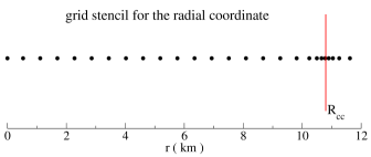
Figure 2: This figure shows the grid stencil for the radial coordinate, which results from the coordinate transformation (46). The refinement of the mesh near the crust/core interface is evident. For clarity, we have shown here a grid with 26 points, while in this work we use 200 points.

5 Numerical method

The numerical code to study the time evolutions of equation (41) is based on the numerical framework developed in Passamonti & Lander (2014). The spatial partial derivatives are approximated by using a second order finite difference scheme, while the evolution in time is performed with an iterative explicit Crank-Nicholson algorithm. To stabilise the simulation we add also a fourth order Oliger-Kreiss numerical dissipation, $\varepsilon_{D}D_{4}\xi$, with a small dissipation coefficient $\varepsilon_{D}\sim 10^{-5}$. The numerical domain covers the 2D-region $0\leq r\leq R$ and $0\leq\theta\leq{\rm\pi}/2$, and the grid resolution used in this work is 200 points in the radial coordinate and 64 points in the angular coordinate.

The crust/core interface is the region where the core and crust oscillations interact, and it is very important to have an adequate grid resolution to describe the wave dynamics. Therefore, we introduce the following transformation to refine the grid around $R_{cc}$:

$$\frac{dr}{dx}=\beta_{r}\,,$$ (45)

where

$$\beta_{r}\equiv 1-a\exp\left[{-\frac{1}{2}\left(\frac{r-r_{0}}{b}\right)^{2}}\right]\,.$$ (46)

We use $a=0.8$, $b=0.5$ km and $r_{0}=10.8$ km, which is close to the actual crust/core transition. Considering an even spaced grid in the x radial coordinate, equation (45) guarantees that the mesh of the r coordinate is finer nearby the crust/core interface (see Fig. 2). The radius of our stellar model in the x-coordinate is $R_{x}=14.54$ km.

To evolve in time the perturbation equation $(\ref{eq:wv})$ in the new grid, we replace the radial derivatives with the following expression:

$$\frac{\partial}{\partial r}\to\frac{1}{\beta_{r}}\frac{\partial}{\partial x}\,,$$ (47)

and the same transformation is applied also to the boundary conditions. We determine the properties of the magneto-elastic modes by post-processing the results of the time simulations. First we get the mode frequencies by using a Fast Fourier Transformation (FFT) of the time evolved Lagrangian displacement $\xi^{\phi}_{\mathrm{c}}$. To monitor the mode pattern we perform an effective FFT on the entire grid by using a code developed by Stergioulas et al. (2004). To study the presence of the continuum spectrum we extract the FFT at different positions inside the star.

6 Results

Several magnetar internal properties (composition, superfluidity, extent of the nuclear pasta region) can influence the QPO spectrum. We begin our discussion by reviewing the main characteristics of the QPOs spectra. We first consider the crustal torsional modes in models without magnetic field, then we study the oscillations in magnetised stars without pasta phases, and finally address the full problem with both magnetic field and pasta configurations.

With respect to superfluidity, the first order effect of the decoupling of the superfluid neutrons from the charged components leads to an increase of the crustal and Alfvén mode frequencies by a factor $x_{\mathrm{c}}^{-1/2}$. This can be seen from the definition of the Alfvén and shear velocities, which in a two-fluid Newtonian system, respectively, read

$$v_{A}=\frac{B}{\sqrt{4\pi\rho_{\mathrm{c}}}}\,,\qquad v_{s}=\sqrt{\frac{\check{\mu}}{\rho_{\mathrm{c}}}}\,,$$ (48)

where the charged particle mass density now replaces the total density appropriate for single fluid stars. However, this frequency increase can be mitigated in the inner crust by the strong entrainment (see Sec. 6.1). The influence of entrainment on the magneto-elastic oscillations has been already studied in Newtonian models by Passamonti & Lander (2013, 2014) and recently in the relativistic case by Gabler et al. (2016). In order not to repeat the same analysis, in this work we consider only the single entrainment configuration which has been described in Sec. 3.4.

Table 1: Frequencies of torsional crustal modes ${}^{l}t_{n}$ (in Hz) for non-magnetised neutron stars. FD and TD correspond to frequencies determined with frequency and time domain approaches, respectively. The second and third columns show the results for a model without entrainment, while the fourth and fifth columns are calculated with the strong entrainment discussed in Sec. 3.4. The sixth column displays the mode frequencies for a non-superfluid (single fluid) star.

Mode	FD	TD	FD	TD	FD
	no entr.	no entr.	with entr.	with entr.	1-fluid
${}^{2}t_{0}$	51.1	51.4	27.4	27.7	25.1
${}^{3}t_{0}$	80.7	81.5	43.2	43.3	39.8
${}^{4}t_{0}$	108.3	108.5	58.0	58.5	53.4
${}^{5}t_{0}$	135.1	135.8	72.4	72.5	66.5
${}^{6}t_{0}$	161.4	161.8	86.5	87.1	79.5
${}^{7}t_{0}$	187.6	188.1	100.5	100.5	92.4
${}^{2}t_{1}$	1388.9	1402.6	891.4	893.2	822.4
${}^{2}t_{2}$	1855.4	1863.2	1424.1	1437.3	1348.2
${}^{2}t_{3}$	2435.5	2488.4	1710.2	1718.2	1659.7

Table 2: Frequencies of the torsional modes ${}^{l}t_{n}$ in Hz for a neutron star model with entrainment, for three different phase transition densities $\rho_{ph}=1,5,10\times 10^{13}\textrm{g cm}^{-3}$. These results are obtained with the FD approach.

		$\rho_{ph}/10^{13}\textrm{g cm}^{-3}$
Mode	10	5	1
${}^{2}t_{0}$	25.0	20.8	16.5
${}^{3}t_{0}$	39.0	32.8	26.1
${}^{4}t_{0}$	53.1	44.0	34.9
${}^{5}t_{0}$	66.3	54.9	43.6
${}^{6}t_{0}$	79.2	65.6	52.1
${}^{7}t_{0}$	92.0	76.2	60.5
${}^{2}t_{1}$	891.1	857.6	690.7
${}^{2}t_{2}$	1422.7	1319.3	1096.0
${}^{2}t_{3}$	1708.2	1936.6	1452.6

6.1 Crustal modes

For testing purposes, we study the torsional shear modes of a non-magnetised star with two methods, the time evolution code and solving a 1D eigenvalue problem (see Appendix B). Our results are reported in Table 1, where we compare the mode frequencies obtained with both our Time Domain (TD) and Frequency Domain (FD) approaches. The results obtained with these two methods agree to better than one percent. As expected, the effect of the high neutron effective mass resulting from entrainment is important. The mode frequency is roughly decreased by a 50 percent with respect to models without entrainment and tend to be closer to the results of non-superfluid stars. In fact, the relative difference of models including entrainment with respect 1-fluid models is about a 10 percent, in agreement with previous works (Samuelsson & Andersson, 2009; Passamonti & Andersson, 2012; Sotani et al., 2013). All the results reported in Table 1 follow the scaling expected for the fundamental modes with respect to the harmonic index $l$ (Samuelsson & Andersson, 2007):

$$\nu\approx\sqrt{\left(l-1\right)\left(l+2\right)}\,.$$ (49)

The effect of the existence of a nuclear pasta layer is shown in Table 2. The mode frequencies decrease with $\rho_{ph}$ (the wider pasta phase region, the lower frequency), as a consequence of the average smaller shear modulus at the bottom of the inner crust (see Fig.1). This trend is in agreement with the results presented in Sotani (2011) and Gearheart et al. (2011).

We use a frequency domain code to determine also the eigenfunctions of the crustal modes. They will be used as initial conditions for the time evolutions of magneto-elastic oscillations. More precisely, we consider the eigenfunctions of the fundamental modes, up to $l=20$, and the first six overtones with $l=2$.

6.2 Magneto-elastic waves

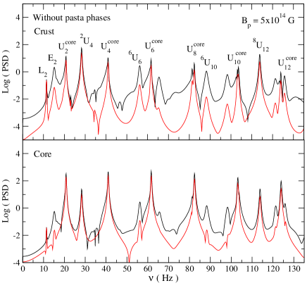
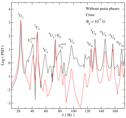
Figure 3: This figure displays the Power Spectrum Density (PSD) of a star without nuclear pasta and with two different magnetic field strength. The left-hand panel shows an FFT taken for a star with $B_{p}=5\times 10^{14}$G in two positions near the magnetic axis, in the crust (upper left-hand panel) and the core (lower left-hand panel). The black line refers to an FFT performed for a 8 s time simulation, while the red line corresponds to the interval $1~{}\textrm{s}<t<8~{}\textrm{s}$. For a model with $B_{p}=10^{15}$G, the right-hand panel shows the results of an FFT performed in the crust near the magnetic axis, for the time interval $0~{}\textrm{s}<t<2~{}\textrm{s}$ (black line) and $0.6~{}\textrm{s}<t<2~{}\textrm{s}$ (red line). The horizontal axis provides the mode frequency in Hz, while the vertical axis the logarithm of the PSD.

The interpretation of the low frequency QPOs as crustal modes drastically depends on the magnetic field strength and the star model. In strongly magnetised stars, crustal modes can live longer if they appear in continuum gaps. This situation is more feasible at low frequencies where the continuum gaps are more likely present (van Hoven & Levin, 2011, 2012). As seen in Sec. 6.1, a way to have a more dense population of shear modes at lower frequencies is to assume an extended nuclear pasta region (low shear) in the inner crust, in the density range $10^{13}\textrm{g cm}^{-3}\lesssim\rho\lesssim 10^{14}\textrm{g cm}^{-3}$ (see e.g. Schneider et al., 2013). Therefore, it is worth investigating whether these modes survive in the spectrum of strongly magnetised stars.

We first study the magneto-elastic oscillations in a neutron star model without nuclear pasta. As described in Sec. 6.1, we initially excite several purely crustal modes and let the system evolve. In this work, we consider a poloidal magnetic field which strength varies in the range $10^{14}$G $\leq B_{p}\leq 2\times 10^{15}$G. To study the properties of the oscillations, we extract the mode frequencies by using the FFT of the time evolved perturbation. We find that for $B_{p}\lesssim 4\times 10^{14}$G, the oscillation modes show the same characteristics of non-superfluid models, which have been thoroughly discussed in the literature. After a transition, where many oscillations of the magnetic field continuum are excited, the spectrum is characterised by the edge modes (vibrations of the last open field lines), the upper modes (mostly localised near the magnetic axis), and the oscillations confined into the closed field line region. For a stronger magnetic field, $B_{p}\gtrsim 5\times 10^{14}$G, there are new features in the spectrum with some of them clearly showing a constant phase character. This kind of magneto-elastic waves have been already found by Gabler et al. (2013) and Passamonti & Lander (2014) and recently studied more extensively by Gabler et al. (2016). One interesting property of these modes is that they are not confined into the core and their amplitude patterns reproduce, in many cases, the longitudinal nodal lines of pure torsional crustal oscillations.

In the literature, there is a proliferation of notation for the mode classification (see Table 1 in Gabler et al., 2016). In this work, we prefer to converge toward the notation recently introduced by Gabler et al. (2016) in order to make easier future comparisons. We denote by E_n and U_n, respectively, the edges and the upper turning points of the continuum bands. The oscillations of the closed magnetic field lines will be labelled as L_n . In addition, we add the superscript ‘core’ to specify the modes which remain mostly confined into the core, while the label $n$ now corresponds to the number of maxima that a mode has along the field lines. For example, in the new notation, an U${}_{2}^{\rm core}$ mode corresponds to the antisymmetric U${}_{0}^{(-)}$ mode of Passamonti & Lander (2014). We label the global magneto-elastic oscillations by ^lU_n, where $n$ denotes, as for the core confined modes, the number of maxima present along the magnetic field lines, while the index $l$ describes the angular structure of the mode pattern. Therefore, a magneto-elastic mode with $l=2$ has the same angular structure of a purely $l=2$ crustal mode.

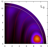
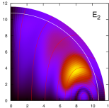
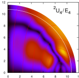
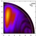
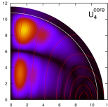
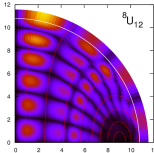
Figure 4: Effective 2D-FFT of six magneto-elastic waves for a model with $B_{p}=5\times 10^{14}$G and without nuclear pasta. We show the absolute value of the amplitude of $\xi^{\phi}$ as determined in the orthonormal basis. From the spectral features of Fig. 3 we select the following modes L₀, E₂, ²U₄/E₄, U${}_{2}^{\rm core}$, U${}_{4}^{\rm core}$, ⁸U₁₂. The magnetic field lines are shown in red, while the crust/core interface with a white line.

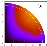
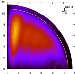
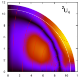
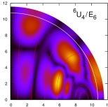
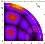
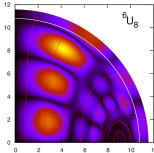
Figure 5: Same as Fig. 4 for $B_{p}=10^{15}$G. The modes selected in this case are ²U₂, U${}_{2}^{\rm core}$, ²U₄ , ⁶U₄ /E₆, ⁶U₆ and ⁶U₈.

For a star with $B_{p}=5\times 10^{14}$G, we show in Fig. 3 an FFT of the Lagrangian displacement taken in two positions near the magnetic axis, in the crust (left-upper panel) and in the core (left-lower panel). To identify the long living oscillations, we have determined the FFT for two different time intervals: the entire evolution $t<8$ s and for $1~{}\textrm{s}<t<8$ s. As pointed out before, many modes are initially excited, but some of them are already significantly damped after one second. The core confined U^core mode, the L modes, and a couple of global magneto-elastic modes (²U₄ and ⁸U₁₂) persist longer and appear to be only weakly damped by numerical dissipation. In particular, the Upper modes are clearly dominant in the core. The 2D patterns of six selected magnetic-elastic modes are shown in Fig. 4. As expected, the E and U^core modes are mainly confined into the core, due to the velocity step present at the crust/core interface, which results in a low efficiency in the transmission of Alfven waves. However, already at this magnetic field strength, the magneto-elastic modes ²U₄ and ⁸U₁₂ have a small damping, as seen in Fig. 3, and clearly reach the surface. In particular, the 2D-pattern of the ²U₄ oscillation shows also the presence of an E₄ mode. Since these two oscillations have similar frequency, the routine that extracts the pattern amplitude from the time simulation is not able to discern between the two modes. Also for the E₂ mode, the 2D pattern indicates the presence of a global oscillation with amplitude much smaller than the edge mode. For stronger magnetic fields, this global oscillation will emerge as an ²U₂ magneto-elastic wave.

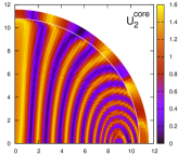
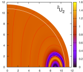
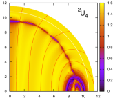
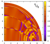
Figure 6: For some of the modes shown in Fig. 5, this figure displays the absolute value of the phase, given in radiants. The star is a model without nuclear pasta and $B_{p}=10^{15}$G. The modes represented are the core confined U${}_{2}^{\rm core}$ mode and the following three global magneto-elastic oscillations ²U₂, ²U₄ and ⁶U₈.

By gradually increasing $B_{p}$, we find that the core confined U modes are less excited while the global magneto-elastic oscillations become dominant. Tracking these modes with varying magnetic field strength, we find that the long-living global magneto-elastic oscillations are actually at the frequency expected for the E_n modes. In our stellar model these two kinds of oscillation modes have similar frequencies. The E_n modes are more excited when the magnetic field is weaker, while the global magneto-elastic oscillations dominate for stronger magnetic fields.

For a star with $B_{p}=10^{15}$G, we show in Fig. 3 an FFT taken close to the magnetic axis and in the crust for two time intervals, $0~{}\textrm{s}<t<2$ s (black line) and $0.6~{}\textrm{s}<t<2$ s (red line), respectively. Several magneto-elastic modes are now excited with different damping times. The 2D patterns (Fig. 5) show that the magneto-elastic oscillations reach the surface and have more angular structure than the core confined U modes. Note that in the ⁶U₄, ⁶U₆ and ⁶U₈ oscillations, the difference between the various local maxima of the amplitude is at most a factor of five.

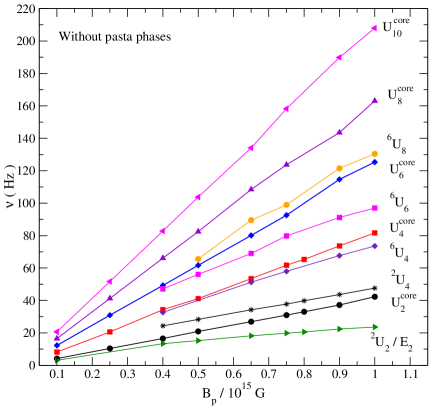
Figure 7: Antisymmetric magneto-elastic modes for a model without nuclear pasta. The figure shows the frequency dependence of several core-confined U-modes and global magneto-elastic oscillations on the magnetic field $B_{p}$ (see legend).

As mentioned above, a way to identify a global oscillation which does not arise from the continuum is to study the oscillation phase (Gabler et al., 2013, 2016). If it is constant, each fluid element oscillates in phase indicating a global coherent character. If instead a mode belongs to the continuum, the fluid element associated with a magnetic field line must oscillate out of phase with the neighbour lines. Calculating the phase of various magneto-elastic oscillations we find some modes which clearly exhibit a coherent character. However, it is not always easy to identify a constant phase in the mode overtones, as other modes with similar frequency can appear in the same pattern and numerical noise might be present around the nodal lines. We show in Fig. 6 the phase of some modes for a star without nuclear pasta and with $B_{p}=10^{15}$G. The core confined U${}_{2}^{\rm core}$ mode exhibits a highly variable phase, while the other global magneto elastic modes, which reach the surface, show a nearly constant phase. This is specially evident for the ²U₂ mode, and less clear for the other two, due to the existence of nodal zones where the amplitude of the oscillation is zero and the color scale does not reflect correctly the phase. It is also seen how the equatorial ring confined into the closed field lines is effectively decoupled from the rest of the star.

Finally, we have checked that the frequency of the magneto-elastic modes scales linearly with the magnetic field strength. By tracking the mode frequency and identifying its 2D-pattern for models with different magnetic field strengths, we find the results shown in Fig. 7. In the explored range, the mode frequencies have a clear linear trend with respect to $B_{p}$. As found also by Gabler et al. (2016) the frequencies of the global magneto-elastic oscillations cannot be determined for $B_{p}<4\times 10^{14}$ G, due to numerical limitation. Therefore, we cannot follow their behaviour for weaker magnetic fields.

To compare our results with the literature, we must determine the relation between the magnetic field at the pole $B_{p}$ and the quantity introduced by Gabler et al. (2016). The authors of this work provide the results as a function of the magnetic field strength, $\bar{B}$, of a uniformly magnetised sphere, which has the same magnetic dipole moment as the stellar model under exam. Furthermore, to rescale the value to a standard model with a radius of 10 km, they used the following equation (Eq. 19 in Gabler et al. (2016))

$$\bar{B}=\frac{m_{dip}}{\left(10~{}\textrm{km}\right)^{3}}\left(\frac{10~{}\textrm{km}}{R}\right)^{2}\,,$$ (50)

where $m_{dip}$ is the magnetic dipole moment of the background model. For the star used in our work Eq. (50) provides $\bar{B}=0.425B_{p}$. For equivalent $\bar{B}$, we find that our results are consistent with those of Gabler et al. (2016). The main characteristics of the oscillation spectrum and the 2D amplitude patterns are very similar. However, we cannot directly compare the oscillation frequencies, because the stellar models used in these two works are different.

6.2.1 Magnetar oscillations with a nuclear pasta layer

Now we discuss the possibility of a region with nuclear pasta phase. In Sec. 3.2 we presented our approximated model for the shear modulus, which smoothy decreases toward the crust/core interface in order to mimic the reduced elasticity expected in the non-uniform pasta structures. We explored a wide range of the pasta phase transition density, $10^{13}\textrm{g cm}^{-3}\leq\rho_{ph}\leq 10^{14}\textrm{g cm}^{-3}$. In general, we find that the excitation of the continuum is more evident during the initial transition period for these models than for models without nuclear pasta, but the system quickly re-distributes the initial energy among the various modes. Depending on the magnetic field strength, the long living modes are the modes at the turning points and edges of the continuum for $B_{p}\lesssim 5\times 10^{14}$G, and the global magneto-elastic modes for stronger magnetic fields, $B_{p}>5\times 10^{15}$G.

Table 3: Frequencies of the antisymmetric magneto-elastic oscillations (in Hz) for a neutron star with entrainment and magnetic field $B_{p}=10^{15}$G. The second column refers to the model without nuclear pasta, while the last three columns present the results for different pasta phase transition densities, $\rho_{ph}=1,5,10\times 10^{13}\textrm{g cm}^{-3}$. These results are determined from the FFT of the time evolution results.

			$\rho_{ph}/10^{13}\textrm{g cm}^{-3}$
Mode	No pasta	10	5	1
2U2	23.8	23.3	22.8	22.1
2U4	47.4	46.1	47.7	47.4
6U4	73.6	72.5	72.8	71.9
6U6	97.1	100.3	93.7	97.3
6U8	125.6	121.6	119.4	120.3
10U8	145.7	137.8	146.8	144.4
10U10	169.4	170.4	171.6	168.6

We focus on a star with $\rho_{ph}=10^{13}\textrm{g cm}^{-3}$, which has the widest nuclear pasta layer within the models considered. In the left panel of Fig. 8, we compare the FFT of the Lagrangian displacement for $B_{p}=5\times 10^{14}$G and $B_{p}=10^{15}$G. The FFTs are taken in the crust near the magnetic axis and in two different time intervals, for the entire evolution $t=2$ s (black line) and for $0.6~{}\textrm{s}<t<2$ s (red line). The main oscillations excited in the star with $B_{p}=5\times 10^{14}$G are clearly the E₂ and U${}_{n}^{\rm core}$ modes. Compared with the model without nuclear pasta, it seems that less magneto-elastic modes are excited in this frequency range (compare Fig. 3 and Fig. 8). For $B_{p}=10^{15}$G (top panel), more magneto-elastic modes show a persistent character or in general a smaller damping than for the $B_{p}=5\times 10^{14}$G case. In the right panel of Fig. 8 we compare the FFTs of two models, with and without pasta phase, with the same magnetic field, $B_{p}=10^{15}$G. The frequency of each magneto-elastic oscillation is quite similar, especially for modes with higher amplitude. In the range $120\textrm{Hz}<\nu<160$ Hz there is a richer spectrum in the model without nuclear pasta, with modes showing more nodal lines along the $\theta$ coordinate (higher harmonic index $l$), but maintaining the same radial structure (see also Fig. 3). It is likely that in some frequency range different initial conditions can excite different overtones, but the frequency of the dominant modes seems to be closer to models without nuclear pasta.

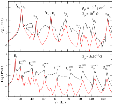
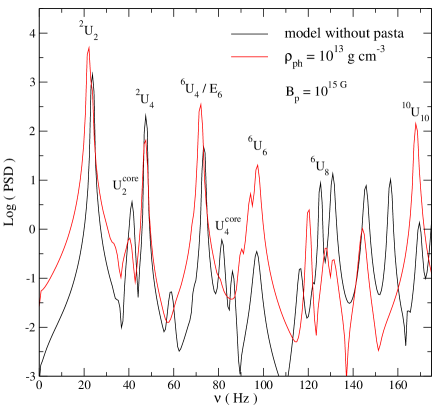
Figure 8: Power spectrum density of a star’s model with nuclear pasta transition $\rho_{ph}=10^{13}~{}\textrm{g cm}^{-3}$. The FFTs are taken in the crust near the magnetic axis. The left-hand panel displays the FFT for the two intervals: $0~{}\textrm{s}\leq t\leq 2~{}\textrm{s}$ (black line) and $0.6~{}\textrm{s}\leq t\leq 2~{}\textrm{s}$ (red line). The star with $B_{p}=5\times 10^{14}$G is shown on the lower-left panel, while the $B_{p}=10^{15}$G case on the upper-left panel. The right-hand panel compares the FFT of a model with $\rho_{ph}=10^{13}~{}\textrm{g cm}^{-3}$ (black line) with a star without nucelar pasta (red line). Both models have $B_{p}=10^{15}$G and the FFT is taken for $0.6~{}\textrm{s}\leq t\leq 2~{}\textrm{s}$.

Considering various models with different $\rho_{ph}$ transition, we find that the spectrum maintains the same basic structure of models without nuclear pasta, and that the frequency of global magneto-elastic modes barely changes with $\rho_{ph}$ (especially for the first three magneto-elastic oscillations). In Table 3 we provide the mode frequencies of the magneto-elastic modes for a model with $B_{p}=10^{15}$G and for different pasta phase transition densities $\rho_{ph}$. We do not show in this table the core confined U modes, as they are less excited into the crust at this magnetic field strength. In any case, their frequencies are very close to those of models without nuclear pasta.

7 Conclusions

The interpretation of magnetar QPOs as driven by the magneto-elastic oscillations is a well established scenario, and it is therefore important to investigate all the physical effects which can modify the oscillation spectrum. In this work we have studied the torsional oscillations of relativistic superfluid magnetars, where the magnetic field has a purely poloidal geometry.

The main properties of the spectrum for stars with and without nuclear pasta are similar to the results obtained by Gabler et al. (2013) and Passamonti & Lander (2014), and consistent with Gabler et al. (2016). In the magnetic field range explored in this work, we find two different families of magneto-elastic modes: a first class of core confined oscillations and a second family of modes which penetrate the crust and reach the surface. The modes of the first class show a no-constant phase and can be associated with the oscillations at the turning points and edges of the continuum bands. The modes which reach the surface have instead a more structured angular pattern which reminds that of the crustal modes, and many of them show a constant phase. We find that these two classes coexist in our simulations, but the core confined modes are dominant at ‘weak’ magnetic fields, typically when $B_{p}\lesssim 4\times 10^{14}$G, while the global magneto-elastic oscillations dominate at stronger magnetic fields, roughly for $B_{p}\gtrsim 5\times 10^{14}$G. Interestingly, if we linearly extrapolate the frequencies of the edge modes for stronger magnetic fields, we find that the magneto-elastic modes with higher amplitude, which persist longer in the evolution, reside close to the edge mode frequency. Imprints of edge modes are in fact found in the 2D oscillation patterns.

Although the crustal modes densely populate, in models with nuclear pasta and strong entrainment, the low frequency part of the spectrum where the continuum gaps are more likely present, we do not find any direct imprints of a fundamental crustal mode for stars with $B_{p}\geq 10^{14}$G. The magneto-elastic oscillations that reach the star’s surface in fact depend linearly on the magnetic field strength. This behaviour should exclude a direct identification of these magneto-elastic modes with purely crustal modes, as the frequency variation for the magneto-corrected crustal modes is very small for the magnetic field strength considered in this work (Sotani et al., 2007; van Hoven & Levin, 2012). Furthermore, the basic structure of the magneto-elastic spectrum does not seem to depend strongly on the presence of nuclear pasta, despite the various models have crustal modes with very different frequencies.

We also explored the high frequency QPOs, around 625 Hz, which can be in the frequency range of the first overtone of torsional crustal modes. Our simulation suggests that the first crustal mode overtone used to excite the time evolution is efficiently absorbed by the continuum when the pasta phase is present and $B_{p}\gtrsim 4\times 10^{14}$G. Therefore the identification of this mode with the 625 Hz QPOs appears more difficult in models with nuclear pasta. This can be due to the smoother transition of the shear modulus across the crust/core interface which facilitates the wave transmission. However, we think that the identification of the high frequency QPOs require a more complex analysis of the spectrum which involves both polar (spheroidal) and axial (torsional) oscillations. This is a key requisite for studying more realistic magnetic field configurations with mixed poloidal-toroidal geometry. With the presence of a toroidal magnetic field component, the polar and axial perturbations couple and the spectrum can change significantly. For instance, there are indications that due to this coupling the continuum spectrum can disappear (Colaiuda & Kokkotas, 2012). This result is in part expected. Works in tokamak and solar physics have in fact shown that the coupling between Alfvén, gravity and pressure waves can open gaps in the continuum bands (see for instance Heidbrink, 2008; Blokland & Keppens, 2011)

Appendix A Wave equation coefficients

We write here the coefficients of the wave equation (41):

$$A_{1} =\check{\mu}\mathrm{e}^{-2\lambda}+\frac{1}{4\pi}\left(B^{r}\right)^{2}\,,$$ (51)

$$A_{2} =\frac{\check{\mu}}{r^{2}}+\frac{1}{4\pi}\left(B^{\theta}\right)^{2}\,,$$ (52)

$$A_{3} =\frac{1}{2\pi}B^{r}B^{\theta}\,,$$ (53)

$$A_{4} =\mathrm{e}^{-2\lambda}\frac{d\check{\mu}}{dr}+\left[\frac{d}{dr}\left(\nu-\lambda\right)+\frac{4}{r}\right]\mathrm{e}^{-2\lambda}\check{\mu}+\frac{1}{4\pi}B^{\theta}\frac{\partial B^{r}}{\partial\theta}$$

$$+\frac{1}{4\pi}\left(\frac{d\nu}{dr}+\frac{2}{r}\right)\left(B^{r}\right)^{2}+\frac{1}{4\pi}\left[2\cot\theta B^{\theta}+\frac{\partial B^{r}}{\partial r}\right]B^{r}\,,$$ (54)

$$A_{5} =\frac{\cot\theta}{r^{2}}\left[3\check{\mu}+\frac{1}{2\pi}\left(B^{\theta}\right)^{2}\right]+\frac{1}{4\pi}\left[\left(\frac{d\nu}{dr}+\frac{2}{r}\right)B^{\theta}+\frac{\partial B^{\theta}}{dr}\right]B^{r}$$

$$+\frac{1}{4\pi}B^{\theta}\frac{\partial B^{\theta}}{\partial\theta}$$ (55)

In the limit of zero shear modulus $\mu=0$, the quantities $A_{k}$ become the coefficients of the wave equation for the core’s protons.

Appendix B Crustal modes

The relativistic equations for studying the crustal torsional modes of a superfluid star have been already derived by Samuelsson & Andersson (2009). By using the harmonic vector expansion the problem becomes a 1D eigenvalue problem. For axisymmetric modes the Lagrangian displacement can be written as following

$$\xi_{\mathrm{c}}^{\phi}=\sum_{l}\frac{\hat{\xi}_{l}}{\sin\theta}\frac{\partial P_{l}}{\partial\theta}\mathrm{e}^{\i\omega_{l}t}\,,$$ (56)

where $\omega_{l}$ is the mode eigenfrequency, $\hat{\xi}_{l}$ is function of $r$, and $P_{l}$ is the Legendre polynomial. The label $l$ denotes the harmonic index. If we introduce the variable expansion (56) into the perturbation equation (41) with zero magnetic field, after some algebra, we find the following equation in the coordinate basis:

$$\check{\mu}\frac{\partial^{2}\hat{\xi}_{l}}{\partial r^{2}}=\left[-\frac{d\check{\mu}}{dr}+\left(\frac{d\lambda}{dr}-\frac{d\nu}{dr}-\frac{4}{r}\right)\check{\mu}\right]\frac{\partial\hat{\xi}_{l}}{\partial r}$$

$$+\left[\left(l+2\right)\left(l-1\right)\frac{\check{\mu}}{r^{2}}-\left(\varepsilon+p\right)\chi\mathrm{e}^{-2\nu}\omega_{l}^{2}\right]\mathrm{e}^{2\lambda}\hat{\xi}_{l}\,.$$ (57)

This equation can be solved as an eigenvalue problem with boundary conditions at the crust/core interface, $r=R_{cc}$, and the star’s surface, $r=R$. In both these boundaries, the continuity of traction leads to the following condition:

$$\frac{\partial\hat{\xi}_{l}}{\partial r}=0\,.$$ (58)

References

- Andersson & Comer (2007) Andersson N., Comer G. L., 2007, Living Reviews in Relativity, 10
- Andersson et al. (2009) Andersson N., Glampedakis K., Samuelsson L., 2009, MNRAS, 396, 894
- Asai & Lee (2014) Asai H., Lee U., 2014, ApJ, 790, 66
- Asai et al. (2015) Asai H., Lee U., Yoshida S., 2015, MNRAS, 449, 3620
- Asai et al. (2016) Asai H., Lee U., Yoshida S., 2016, MNRAS, 455, 2228
- Blokland & Keppens (2011) Blokland J. W. S., Keppens R., 2011, AA, 532, A94
- Caplan et al. (2015) Caplan M. E., Schneider A. S., Horowitz C. J., Berry D. K., 2015, Phys. Rev. C, 91, 065802
- Carter (1989) Carter B., 1989, Lecture Notes in Mathematics, Berlin Springer Verlag, 1385, 1
- Carter & Langlois (1998) Carter B., Langlois D., 1998, Nuclear Physics B, 531, 478
- Carter & Quintana (1972) Carter B., Quintana H., 1972, Proceedings of the Royal Society of London Series A, 331, 57
- Carter & Samuelsson (2006) Carter B., Samuelsson L., 2006, Class. and Quantum Grav., 23, 5367
- Chamel (2005) Chamel N., 2005, Nucl. Phys. A, 747, 109
- Chamel (2006) Chamel N., 2006, Nucl. Phys. A, 773, 263
- Chamel (2008) Chamel N., 2008, MNRAS, 388, 737
- Chamel (2012) Chamel N., 2012, Phys. Rev. C, 85, 035801
- Chamel & Haensel (2008) Chamel N., Haensel P., 2008, Living Reviews in Relativity, 11
- Colaiuda et al. (2009) Colaiuda A., Beyer H., Kokkotas K. D., 2009, MNRAS, 396, 1441
- Colaiuda & Kokkotas (2011) Colaiuda A., Kokkotas K. D., 2011, MNRAS, 414, 3014
- Colaiuda & Kokkotas (2012) Colaiuda A., Kokkotas K. D., 2012, MNRAS, 423, 811
- Douchin & Haensel (2000) Douchin F., Haensel P., 2000, Phys. Lett. B, 485, 107
- Douchin & Haensel (2001) Douchin F., Haensel P., 2001, AA, 380, 151
- Duncan (1998) Duncan R. C., 1998, ApJ, 498, L45
- Fantina et al. (2012) Fantina A. F., Chamel N., Pearson J. M., Goriely S., 2012, Journal of Physics Conference Series, 342, 012003
- Gabler et al. (2011) Gabler M., Cerdá Durán P., Font J. A., Müller E., Stergioulas N., 2011, MNRAS, 410, L37
- Gabler et al. (2013) Gabler M., Cerdá-Durán P., Font J. A., Müller E., Stergioulas N., 2013, MNRAS, 430, 1811
- Gabler et al. (2012) Gabler M., Cerdá-Durán P., Stergioulas N., Font J. A., Müller E., 2012, MNRAS, 421, 2054
- Gabler et al. (2013) Gabler M., Cerdá-Durán P., Stergioulas N., Font J. A., Müller E., 2013, Phys. Rev. Lett., 111, 211102
- Gabler et al. (2014) Gabler M., Cerdá-Durán P., Stergioulas N., Font J. A., Müller E., 2014, MNRAS, 443, 1416
- Gabler et al. (2016) Gabler M., Cerdá-Durán P., Stergioulas N., Font J. A., Müller E., 2016, MNRAStmp..954G
- Gearheart et al. (2011) Gearheart M., Newton W. G., Hooker J., Li B.-A., 2011, MNRAS, 418, 2343
- Glampedakis et al. (2006) Glampedakis K., Samuelsson L., Andersson N., 2006, MNRAS, 371, L74
- Heidbrink (2008) Heidbrink W. W., 2008, Physics of Plasmas, 15, 055501
- Horowitz et al. (2015) Horowitz C. J., Berry D. K., Briggs C. M., Clapan M. E., Cumming A., Schneider A. S., 2015, Phys. Rev. Lett., 114, 031102
- Huppenkothen et al. (2014a) Huppenkothen D., et al., 2014, ApJ, 787, 128
- Huppenkothen et al. (2014b) Huppenkothen D., Heil L. M., Watts A. L., Göğüş E., 2014, ApJ, 795, 114
- Huppenkothen et al. (2014) Huppenkothen D., Watts A. L., Levin Y., 2014, ApJ, 793, 129
- Israel et al. (2005) Israel G. L., Belloni T., Stella L., Rephaeli Y., Gruber D. E., Casella P., Dall’Osso S., Rea N., Persic M., Rothschild R. E., 2005, ApJ, 628, L53
- Karlovini & Samuelsson (2003) Karlovini M., Samuelsson L., 2003, Class. and Quantum Grav., 20, 3613
- Lee (2008) Lee U., 2008, MNRAS, 385, 2069
- Levin (2006) Levin Y., 2006, MNRAS, 368, L35
- Levin (2007) Levin Y., 2007, MNRAS, 377, 159
- Link (2014) Link B., 2014, MNRAS, 441, 2676
- Link & van Eysden (2015) Link B., van Eysden C. A., 2015, ArXiv e-prints
- Mereghetti (2008) Mereghetti S., 2008, AA Rev., 15, 225
- Passamonti & Andersson (2012) Passamonti A., Andersson N., 2012, MNRAS, 419, 638
- Passamonti & Lander (2013) Passamonti A., Lander S. K., 2013, MNRAS, 429, 767
- Passamonti & Lander (2014) Passamonti A., Lander S. K., 2014, MNRAS, 438, 156
- Pethick & Potekhin (1998) Pethick C. J., Potekhin A. Y., 1998, Physics Letters B, 427, 7
- Potekhin et al. (2013) Potekhin A. Y., Fantina A. F., Chamel N., Pearson J. M., Goriely S., 2013, AA, 560, A48
- Samuelsson & Andersson (2007) Samuelsson L., Andersson N., 2007, MNRAS, 374, 256
- Samuelsson & Andersson (2009) Samuelsson L., Andersson N., 2009, Class. and Quantum Grav., 26, 155016
- Schneider et al. (2013) Schneider A. S., Horowitz C. J., Hughto J., Berry D. K., 2013, Phys. Rev. C, 88, 065807
- Sharma et al. (2015) Sharma B. K., Centelles M., Viñas X., Baldo M., Burgio G. F., 2015, AA, 584, A103
- Sinha & Sedrakian (2014) Sinha M., Sedrakian A., 2014, ArXiv e-prints
- Sotani (2011) Sotani H., 2011, MNRAS, 417, L70
- Sotani (2015) Sotani H., 2015, Phys. Rev. D, 92, 104024
- Sotani et al. (2007) Sotani H., Kokkotas K. D., Stergioulas N., 2007, MNRAS, 375, 261
- Sotani et al. (2008) Sotani H., Kokkotas K. D., Stergioulas N., 2008, MNRAS, 385, L5
- Sotani et al. (2013) Sotani H., Nakazato K., Iida K., Oyamatsu K., 2013, MNRAS, 428, L21
- Stergioulas et al. (2004) Stergioulas N., Apostolatos T. A., Font J. A., 2004, MNRAS, 352, 1089
- Strohmayer et al. (1991) Strohmayer T., van Horn H. M., Ogata S., Iyetomi H., Ichimaru S., 1991, ApJ, 375, 679
- Strohmayer & Watts (2005) Strohmayer T. E., Watts A. L., 2005, ApJ, 632, L111
- van Hoven & Levin (2008) van Hoven M., Levin Y., 2008, MNRAS, 391, 283
- van Hoven & Levin (2011) van Hoven M., Levin Y., 2011, MNRAS, 410, 1036
- van Hoven & Levin (2012) van Hoven M., Levin Y., 2012, MNRAS, 420, 3035
- Watts & Strohmayer (2006) Watts A. L., Strohmayer T. E., 2006, ApJ, 637, L117