The Application of Mutual Energy Theorem in Expansion of Radiation Field in Spherical Waves

Abstract

“Mutual energy theorem” and the concept of inner product of electromagnetic fields are introduced, on which the method of expansion of radiation field in spherical waves is discussed.

I introduction

In recent years the spherical wave expansion method has been widely applied to the theory and calculation of electromagnetic fields. But the inner product exist in referenceAWRudge is defined on the Banach spaceWeixingZheng . Through redefining the inner product this article limits the wave expansion method to Hibert spaceDCStinson . For this reason the mutual energy theorem is introduced.

II The definition of the inner product and wave expansions

The electromagnetic fields in the space can be seen as an element which can be expressed as,

$$\zeta=\{E,H\}$$ (1)

All the electromagnetic fields in the space compose a set which can be written as $Q$. In practices that $Q$ is the solution set of the Maxwell’s equations:

$$\{\zeta|\nabla\times E=-j\omega\mu H-K,\nabla\times H=j\omega\epsilon E+J\}$$ (2)

where $K$ is the intensity of the magnetic current, $J$ is the intensity of current, $\omega$ is the frequency, $\epsilon$,$\mu$ are real number (also can be complex number, noticed by the translator), which are permittivity and permeability. $Q$ is a linear space in practical.

Assume there is a volume $V$ in the space, which has the boundary $\varGamma$ . Assume the field $\zeta$ is produced by $J$ and $K$, then all this kind of elements compose a subspace $G$ (Assume $\zeta$ belong to the retarded potential, there is no advanced potential, noticed by the translator). The inner product can be defined on $G$,

$$(\zeta_{1},\zeta_{2})=\oiintop_{\varGamma}\,(E_{1}\times H_{2}^{*}+E_{2}^{*}\times H_{1})\,\hat{n}\,ds$$ (3)

where, $\zeta_{i}=\{E_{i},H_{i}\}$, $i=1,2$, $\hat{n}$ is the normal vector direct to the outside of the surface $\varGamma$, The symbol $*$ expresses the complex conjugate. This inner product satisfies the inner product laws:

(I) $(\zeta,\zeta)\geq 0,\ \zeta=0\ \ \ iff\ (\zeta,\zeta)=0$

(II) $(\zeta_{1},\zeta_{2})=(\zeta_{2},\zeta_{1})^{*}$

(III) $(\alpha\zeta_{1}+\beta\zeta_{2},\zeta_{3})=\alpha(\zeta_{1},\zeta_{3})+\beta(\zeta_{2},\zeta_{3})$

Where $iff$ means “if and only if”; $\alpha$,$\beta$ are any constants, $\zeta_{1}$, $\zeta_{2}$, $\zeta_{3}$$\in G$.

If the above definition of inner product is widened from $G$ to $Q$, the law (I) does not satisfy. Hence on the linear space $Q$, the inner product can only been seen as a generalized definition of the inner product.

From this definition of the inner product, the definition of the norm is,

$$||\zeta||=\sqrt{(\zeta,\zeta)}=(2\,Re\oiintop_{\varGamma}E\times H^{*}\cdot\hat{n}ds)^{\frac{1}{2}}$$ (4)

In the above formula, $Re$ means “taking real part”.

Assume that $\{\zeta_{\lambda}\}$ is a complete set on $G$. Here $\lambda\in\Lambda$, $\Lambda$ is a index set, which satisfies the normalized orthogonal condition,

$$(\zeta_{\mu,}\zeta_{\nu})=\delta_{\mu\nu}\ \ \ \ \ (\mu,\nu\in\Lambda)$$ (5)

where, $\delta_{\mu\nu}$ is Kronecker operator. For any $\zeta\in G$ there is

$$\zeta=\sum_{\lambda\in\Lambda}c_{\lambda}\zeta_{\lambda}$$ (6)

where the expansion coefficient can be found as $c_{\lambda}=(\zeta,\zeta_{\lambda})$.

For spherical expansion, $\{\zeta_{\lambda}\}$ is chosen as spherical wave function, in this case $\lambda$ means $nm$, $\zeta_{\lambda}$ have two forms $\xi_{nm},\eta_{nm}$, where

$$\xi_{nm}=\{M_{nm},\frac{j}{\eta}N_{nm}\}$$ (7)

$$\eta_{nm}=\{N_{nm},\frac{j}{\eta}M_{nm}\}$$ (8)

where the constant factor $\frac{j}{\eta}$ make the above formula so that if the first item inside the brace $\{\}$ is electric field, the second will correspond to the magnetic field. $M_{nm}=\nabla\times[g_{n}\vec{r}h_{n}(kr)Y_{n}^{m}(\theta,\varphi)$, $N_{nm}=\frac{1}{K}\nabla\times M_{nm}$. $h_{n}$ is $n$ level class II spherical Hankel function. $k=\omega\sqrt{\epsilon\mu}$, $\eta=(\mu/\epsilon)^{\frac{1}{2}}$, $g_{n}$ is a normalized constant which will be found later. $r,\theta$ and $\varphi$ are spherical coordinates. The corresponding unit vector are $\hat{r}$, $\hat{\theta}$, $\hat{\varphi}$, but $\vec{r}=r\hat{r}$, $Y_{n}^{m}$are $nm$ level spherical function,

$$Y_{n}^{m}(\theta,\varphi)=[(2n+1)\frac{(n-m)!}{(n+m)!}]^{\frac{1}{2}}P_{n}^{m}(\cos\theta)e^{jm\varphi}$$ (9)

where, $P_{n}^{m}$ is associated Legendre function, $n=0,1\cdots\cdots,$ $m=\pm 0,\pm 1\cdots\cdots\pm n$.

If the normalized orthogonal are established for the spherical wave, Eq.(6) can be rewritten as,

$$\left\{\begin{array}[]{c}\zeta=\sum_{nm}(a_{nm}\xi_{nm}+b_{nm}\eta_{nm}\\ a_{nm}=(\zeta,\xi_{nm}),\ \ b_{nm}=(\zeta,\eta_{nm})\end{array}\right\}$$ (10)

III The orthogonalization and normalization of the spherical wave

It can be seen from Eq.(4) that, if the sources of $\zeta$ is inside the surface $\varGamma$, i.e. $\zeta\in G$, the norm $||\zeta||$ is only the power flow to the outside of $\varGamma$. If the media are lossless, then the power of $\zeta$ is not changed to different surface $\varGamma$. Considering a surface $\varGamma$ with arbitrary radio, we can obtain from the calculation[3] that,

$$||\zeta_{\lambda}||^{2}=||\xi_{nm}||^{2}=||\eta_{nm}||^{2}=\frac{8\pi}{\eta k^{2}}n(n+1)g_{n}$$ (11)

Considering the normalization condition $||\zeta_{\lambda}||=1$, the normalization constant can be obtained

$$g_{n}=k\sqrt{\frac{\eta}{8\pi(n+1)}}$$ (12)

For convenience, the spherical wave is divided to

$$\begin{cases}\xi_{nm}=\xi_{nm}^{(1)}+\xi_{nm}^{(2)}\\ \eta_{nm}=\eta_{nm}^{(1)}+\eta_{nm}^{(2)}\end{cases}$$ (13)

$$\begin{cases}\xi_{nm}^{(i)}=\{M_{nm}^{(i)},\frac{j}{\eta}N_{nm}^{(i)}\}\\ \eta_{nm}^{(i)}=\{N_{nm}^{(i)},\frac{j}{\eta}M_{nm}^{(i)}\}\end{cases}(i=1,2)$$ (14)

(Notice: I have corrected the print error in the above formula, in the original publication, $\xi_{nm}^{(i)}$ is written as $\xi_{1}^{(i)}$ and $\eta_{nm}^{(i)}$ is written as $\eta^{(i)}$, noticed by the translator.)

$$\begin{cases}M_{nm}^{(1)}=\nabla\times[g_{n}\overrightarrow{r}j_{n}(kr)Y_{n}^{m}(\theta,\varphi)\\ M_{nm}^{(2)}=\nabla\times[-jg_{n}\overrightarrow{r}\,n_{n}(kr)Y_{n}^{m}(\theta,\varphi)\\ N_{nm}^{(i)}=\frac{1}{k}\nabla\times M_{nm}^{(i)}&(i=1,2)\end{cases}$$ (15)

Actually the above is that the second class spherical Hankel function $h_{n}(kr)=j_{n}(kr)-jn_{n}(kr)$ in the wave function is divided to two items. $j_{n}$,$n_{n}$ are first class and second class spherical Bessel functions.

According to Eq.(12) and referenceAWRudge it can be proven that the spherical wave are orthogonal

$$(\xi_{nm},\xi_{ts})=\delta_{nt}\delta_{ms}$$ (16)

$$(\xi_{nm},\xi_{ts}^{(i)})=(\xi_{nm},\xi_{ts}^{(i)})=\frac{1}{2}\delta_{nt}\delta_{ms}\ \ \ \ \ \ (i=1,2)$$ (17)

$$(\xi_{nm}^{(i)},\eta_{ts}^{(j)})=0$$ (18)

In the above 3 formula $n$, $m$, $t$, $s$ are integer. in Eq.(18) $i$,$j$ are $1,2$ or no superscript.

IV The mutual energy theorem and the modified mutual energy theorem

A theorem is introduced, which is referred as the mutual energy theorem

$$\oiint_{\Gamma}(E_{1}\times H_{2}^{*}+E_{2}^{*}\times H_{1})\,\hat{n}dS$$

$$=-\intop_{V}(J_{1}\cdot E_{2}^{*}+K_{1}\cdot H_{2}^{*}+J_{2}^{*}\cdot E_{1}+K_{2}^{*}\cdot H_{1})\,dV$$ (19)

In the above formula $\varGamma$ is the boundary of volume $V$. $\hat{n}$, normal vector directed to the outside of surface $\varGamma$. $J_{1},K_{1}$and $J_{2},K_{2}$ are the sources of field $E_{1},H_{1}$ and $E_{1},H_{2}$. This theorem is established in the lossless media, that is if the media satisfies that,

$$\overleftrightarrow{\epsilon}=(\overleftrightarrow{\epsilon})^{\dagger}\ \ \ \ \ \ \ \overleftrightarrow{\mu}=(\overleftrightarrow{\mu}){}^{\dagger}$$ (20)

In the above formula, the superscript $\dagger$ is matrix transpose and complex conjugate. This theorem is proven in the following.

Recent year in the four wave frequency mixing theoryPeiXuanYie , the concept of conjugate wave has been applied. This concept can be summarized as conjugate transform.

If $E,H$ satisfy the Maxwell’s equations

$$\nabla\times E=-j\omega\overleftrightarrow{\mu}H-K\ \ \ \ \ \ \ \nabla\times H=+j\omega\overleftrightarrow{\epsilon}E+J$$ (21)

Then take the transform $E=E^{b*}$, $H=-H^{b*}$, $K=K^{b*},$ $J=-J^{b*}$, $\overleftrightarrow{\epsilon}=(\overleftrightarrow{\epsilon})^{b*}$, $\overleftrightarrow{\mu}=(\overleftrightarrow{\mu})^{b*}$, $E^{b},H^{b}$ still satisfy the Maxwell’s Equations Eq.(21). Hence this transform is referred as conjugate transform.

To the variable with subscript $2$ in the reversible theorem in referenceJAKong make the conjugate transform the modified mutual energy theorem can be obtained.

$$\oiint_{\Gamma}(E_{1}\times H_{2}^{d*}+E_{2}^{d*}\times H_{1})\,\hat{n}dS$$

$$=-\intop_{V}(J_{1}\cdot E_{2}^{d*}+K_{1}\cdot H_{2}^{d*}+J_{2}^{d*}\cdot E_{1}+K_{2}^{d*}\cdot H_{1})\,dV$$ (22)

In the above formula $E_{2}^{d},H_{2}^{d}$ satisfy Maxwell’s equation with the associate media $(\overleftrightarrow{\epsilon})^{d}$, $(\overleftrightarrow{\epsilon})^{d}$. Here

$$(\overleftrightarrow{\epsilon})^{d}=(\overleftrightarrow{\epsilon})^{\dagger}$$

$$(\overleftrightarrow{\mu})^{d}=(\overleftrightarrow{\mu})^{\dagger}$$

If the media is lossless, i.e. Eq(20) is established, then the associated media is same to the original media, ($(\overleftrightarrow{\epsilon})^{d}=\overleftrightarrow{\epsilon},\ (\overleftrightarrow{\mu})^{d}=\overleftrightarrow{\mu}$). In this time the modified mutual energy theorem become the mutual energy theorem Eq.(19).

In the following assume the media are isotropic. Hence the tensors permittivity $\overleftrightarrow{\epsilon}$ and permeability $\overleftrightarrow{\mu}$ become constant permittivity $\epsilon$ and permeability $\mu$.

V The formula for the coefficient of the spherical wave expansion

V.1 Obtaining the coefficients of the spherical expansion knowing the current distribution

Assume the source of radiation is the current distribution $J$, $J$ is inside the spherical surface $\varGamma$. Apply the mutual energy theorem on $\varGamma$, we can obtain,

$$c_{\lambda}=(\zeta,\zeta_{\lambda})=\oiintop_{\varGamma}\ (E\times H_{\lambda}^{*}+E_{\lambda}^{*}\times H)\,\hat{n}ds$$

$$-\intop_{V}E_{\lambda}^{*}\cdot J\,dv-\oiintop_{\varGamma_{\delta}}\,(E\cdot J_{\lambda}^{*}+H\cdot K_{\lambda}^{*})\,ds$$ (23)

In the above formula $\zeta_{\lambda}=\{E,H\}$, and $E_{\lambda}=M_{nm}$ or $N_{nm}$, $J_{\lambda}$and $K_{\lambda}$are effective current and magnetic current sources of the filed $\zeta_{\lambda}$. They are distributed on the spherical surface $\varGamma_{\delta}$ which has radio $\delta\rightarrow 0$ and its center at the oringin $O$. (Notice, according to the mutual energy theorem formula Eq.(19) the integral $\oiintop_{\varGamma_{\delta}}\,(E\cdot J_{\lambda}^{*}+H\cdot K_{\lambda}^{*})\,ds$ is an integral on a volume $V_{\delta}$, the boundary surface of the volume $V_{\delta}$ is $\varGamma_{\delta}$; in the limit situation, the volume integral changed to surface integral. Noticed by the translator.)

For the special situation that the field $\zeta=\{E,H\}$ is just zero at the epsilon neighborhood to origin, the last item of the formula Eq.(23) vanishes. This situation same as the origin is chosen inside the antenna, the antenna can be seen as ideal electric conductor. In this situation there are

$$\begin{cases}c_{\lambda}=-\intop_{V}E_{\lambda}^{*}J\,dv\\ a_{nm}=-\intop_{V}M_{nm}^{*}J\,dv\\ b_{nm}=-\intop_{V}N_{nm}^{*}J\,dv\end{cases}$$ (24)

In case in the epsilon neighborhood the field is not zero, in the Eq.(23) can have integral divergence. In order to overcome this difficulty, assume that the effective source $J_{\lambda}$, $K_{\lambda}$ produce the filed outside of the surface $\varGamma_{\lambda}$ is $\zeta_{\lambda}$, and inside the $\varGamma_{\lambda}$ is $\zeta_{\lambda}^{(1)}$. $\zeta_{\lambda}^{(1)}=\xi_{nm}^{(1)}$ or $\eta_{nm}^{(1)}$ which is given through Eq.(14).

According to effective principle that the effective source can be written as

$$\begin{cases}J_{\lambda}=\hat{n}_{\lambda}\times(H_{\lambda}-H_{\lambda}^{(1)})=\hat{n}_{\lambda}\times H^{(2)}\\ K_{\lambda}=-\hat{n}_{\lambda}\times(E_{\lambda}-E_{\lambda}^{(1)})=-\hat{n}_{\lambda}\times E_{\lambda}^{(2)}\end{cases}$$ (25)

In the above formula, $\hat{n}_{\lambda}$ is outside direction normal vector of the spherical surface $\varGamma_{\lambda}$. $\zeta_{\lambda}^{(2)}=(E_{\lambda}^{(2)},H_{\lambda}^{(2)})$ can be calculated through Eq.(14). The source distribution can be seen in Figure 1.

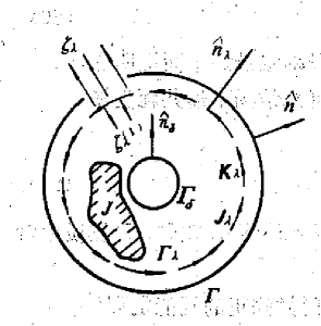
Figure 1: Effective Source $J_{\lambda},$$K_{\lambda}$, radiation source $J$, and the surface $\varGamma$,$\varGamma_{\delta}$,$\varGamma_{\lambda}$.

This way the effective source $J_{\lambda}$, $K_{\lambda}$can create transmission wave at outside the spherical surface and produce standing wave inside the shperical surface. Apply mutual energy theorem on the spherical surface $\varGamma$ can obtain,

$$c_{\lambda}=(\zeta,\zeta_{\lambda})=\oiintop_{\varGamma}\,(E\times H_{\lambda}^{*}+E_{\lambda}^{*}\times H)\cdot\hat{n}ds$$

$$=-\intop_{V}E_{\lambda}^{(1)}\cdot Jdv-\oiintop_{\varGamma_{\lambda}}\,(E\cdot J_{\lambda}^{*}+H\cdot K_{\lambda}^{*})\,ds$$ (26)

(Notice, $E_{\lambda}^{(1)}$, $H_{\lambda}^{(1)}$ are transmission waves, $E_{\lambda}^{(2)}$, $H_{\lambda}^{(2)}$ are stand vaves, Noticed by the translator)

Considering Eq.(25), the last item in the above formula is,

$$-\oiintop_{\varGamma_{\lambda}}(E^{*}\cdot J_{\lambda}+H^{*}\cdot K_{\lambda})\,ds=(\zeta,\zeta_{\lambda}^{(2)})$$ (27)

And from orthogonal condition Eq.(17) we can obtain,

$$(\zeta,\zeta_{\lambda}^{(2)})=(\sum_{\lambda\in\Lambda}c_{\lambda}\zeta_{\lambda},\zeta_{\lambda}^{(2)})=\frac{1}{2}c_{\lambda}$$ (28)

Substituting Eq(27), Eq.(28) to Eq(26) and after arrangement we obtain,

$$\begin{cases}c_{\lambda}=-2\intop_{V}E_{\lambda}^{(1)*}\cdot J\,dv\\ a_{nm}=-2\intop_{V}M_{nm}^{(1)*}\cdot J\,dv\\ b_{nm}=-2\intop_{V}N_{nm}^{(1)*}\cdot J\,dv\end{cases}$$ (29)

This result is same as referenceCHPapas .

V.2 the coefficients of the spherical expansion knowing the tangential component of the electromagnetic fields

Assume there is radiation source current intensity $J$ inside the sphere $\varGamma$. This source produce the field $\zeta=\{E,H\}$. We have measured the tangent filed on the spherical surface $\varGamma$. The wave can be expanded as spherical wave, the spherical wave coefficients are,

$$\begin{cases}a_{nm}=\oiintop_{\varGamma}[-\frac{j}{\eta}(E_{\theta}N_{nm\varphi}^{*}-E_{\varphi}N_{nm\theta}^{*})-H_{\theta}M_{nm\varphi}^{*}+H_{\varphi}M_{nm\theta}^{*}]ds\\ b_{nm}=\oiintop_{\varGamma}[-\frac{j}{\eta}(E_{\theta}M_{nm\varphi}^{*}-E_{\varphi}M_{nm\theta}^{*})-H_{\theta}N_{nm\varphi}^{*}+H{}_{\varphi}N_{nm\theta}^{*}]ds\end{cases}$$ (30)

In the above formula, $X_{\theta}$$X_{\varphi}$ are tangential component of $X$ in $\theta$ and $\varphi$ direction.

V.3 The method to find the coefficients of the spherical wave expansion for the radiation sources when there exist the interference sources

Assume there radiation source $J$ and the interference source $J_{g}$. The corresponding field is $\zeta_{g}=\{E_{g},H_{g}\}$. Chosen the sphere $\varGamma$ so that $J$ is inside $\varGamma$, $J_{g}$ is outside the $\varGamma$. Let the sum of $J$ and $J_{g}$ is $J^{\prime}$, the corresponding field is $\zeta^{\prime}=\{E^{\prime},H^{\prime}\}$. In the boundary $\varGamma$ measured that the tangential field of $E^{\prime}$ and $H^{\prime}$.

$\varGamma_{\lambda}$ is the source of spherical wave $\zeta_{\lambda}$. $\varGamma_{\lambda}$ is chosen at the outside of the spherical surface $\varGamma$ but let the interference source be at the outside of $\varGamma_{\lambda}$. In this situation the effective source still can be given by Eq.(25). This way $J_{\lambda}$ , $K_{\lambda}$will produce the field $\zeta_{\lambda}^{(1)}$ inside the spherical surface $\varGamma_{\lambda}$ and produce the field $\zeta_{\lambda}$ outside the spherical surface $\varGamma_{\lambda}$. All sources and fields and surfaces can be seen in Figure 2.

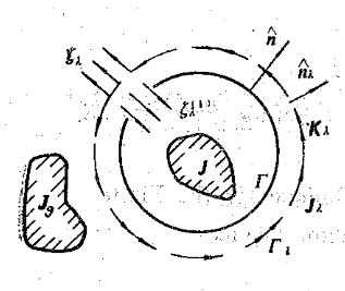
Figure 2: The effective source $J_{\lambda},$$K_{\lambda},$ radiation source $J$, and the interference source $J_{g}$

Taking the inner product at the surface $\varGamma$ and considering the orthogonal formula Eq.(17), we can obtain,

$$(\zeta,\zeta_{\lambda}^{(1)})=(\sum_{\lambda\in\Lambda}c_{\lambda}\zeta_{\lambda,}\zeta_{\lambda}^{(1)})=\frac{1}{2}c_{\lambda}$$ (31)

Because the radiation field $\zeta=\zeta^{\prime}-\zeta_{g}$, there is,

$$(\zeta,\zeta_{\lambda}^{(1)})=(\zeta^{\prime},\zeta_{\lambda}^{(1)})-(\zeta_{g},\zeta_{\lambda}^{(1)})$$ (32)

Considering inside the spherical surface $\varGamma$, $J_{g}$ which is the the source of field $\zeta_{g}$ and effective source $J_{\lambda}$and $K_{\lambda}$are all vanishes, according to the mutual energy theorem Eq.(19) the last item of Eq.(32) vanishes:

$$(\zeta_{g},\zeta_{\lambda}^{(1)})=\oiintop_{\varGamma}\,(E_{g}\times H_{\lambda}^{(1)*}+E_{\lambda}^{(1)*}\times H_{g})\cdot\hat{n}ds=0$$ (33)

Hence, there is

$$c_{\lambda}=2(\zeta^{\prime},\zeta_{\lambda}^{(1)})$$ (34)

$$\begin{cases}a_{nm}=2\oiintop_{\varGamma}[-\frac{j}{\eta}(-E^{\prime}_{\theta}N_{nm\varphi}^{(1)*}-E^{\prime}_{\varphi}N_{nm\theta}^{(1)*})-H_{\theta}^{\prime}M_{nm\varphi}^{(1)*}+H^{\prime}_{\varphi}M_{nm\theta}^{(1)*}]ds\\ b_{nm}=2\oiintop_{\varGamma}[-\frac{j}{\eta}(-E^{\prime}_{\theta}M_{nm\varphi}^{(1)*}-E^{\prime}_{\varphi}M_{nm\theta}^{(1)*})-H_{\theta}^{\prime}N_{nm\varphi}^{(1)*}+H^{\prime}_{\varphi}N_{nm\theta}^{(1)*}]ds\end{cases}$$ (35)

Comparing with Eq.(30), the advantage of Eq.(35) is that there is no influence of the obtained coefficient of the spherical wave expansion with the interference sources.

For the problem of measurement of scattering field, this result can be applied. The incident field and the scattering field can be seen as interference field and the radiation field. This way the calculation of the expansion coefficient of the spherical wave for the scattering field can directly use the formula Eq.(35) . Hence if the superimposed field of the incident field and the scattering field have been measured, the scattering field can be calculate at the outside of the spherical surface $\Gamma$.

VI Conclusion

When making spherical expansion, handiness apply mutual energy theorem can simplify the derivation process and make the physical meaning clearer. All the more so in the case the influence of the interference source must be considered.

References

• (1) A. W. Rudge: The Handbook of Antenna Design, Volume 1. Peter Peregrinus Ltd. London UK, pp. 101-124, 1982.
• (2) Weixing Zheng, the analysis outline of the real function and functional, the people publishing firm, PP 159l-181, 1980.
• (3) Donald C. Stinson: Intermediate Mathmatics of electromagnetics, Enlewood Cliffs N. J., Prentide-Hall, pp. 271,1976.
• (4) J. A. Kong: Electromagnetic field, the people publishing firm, pp. 499-504, 1985.
• (5) Peixuan Ye, Physics, Vol. 14, pp. 499-504, 1985.
• (6) C. H. Papas: Theory of electromagnetic wave Propagation, New York, McGraw-Hill, pp. 97-108, 1965.