Photo-modulation of the spin Hall conductivity of mono-layer transition metal dichalcogenides

Abstract

We report on a possible optical tuning of the spin Hall conductivity in mono-layer transition metal dichalcogenides. Light beams of frequencies much higher than the energy scale of the system (the off-resonant condition) does not excite electrons but rearranges the band structure. The rearrangement is quantitatively established using the Floquet formalism. For such a system of mono-layer transition metal dichalcogenides, the spin Hall conductivity (calculated with the Kubo expression in presence of disorder) exhibits a drop at higher frequencies and lower intensities. Finally, we compare the spin Hall conductivity of the higher spin-orbit coupled WSe₂ to MoS₂; the spin Hall conductivity of WSe₂ was found to be larger.

The transition metal dichalcogenides (TMDCs) are layered materials of covalently bonded atoms held together by weak van der Waals forces Wang et al. (2012) and represented by the formula MX₂ where M is a transition metal element from group IV-VI while X denotes the chalcogens S, Se, and Te. The bulk TMDC when mechanically exfoliated gives a layered two-dimensional configuration of atoms with distinct characteristics. Huang et al. (2013) For instance, a single layer of TMDC has high electron mobility, a direct band gap, absence of dangling bonds and can be stacked in vertical layers Lee et al. (2013) to form hetero-junctions with clean interfaces. The dispersion of a single layer of TMDC also supports a rich variety of condensed matter phenomena, notably the coupling of the valley and electron spin degree of freedom Xiao et al. (2012) without an external magnetic field. The coupling of the spin and valley degree of freedom is most easily observed at the time reversed pair of valley-edges K and K${}^{{}^{\prime}}$ and in their immediate vicinity. Interestingly, this dispersion, as shown in Ref. Tahir et al., 2014 can be modulated by light under off-resonant conditions López et al. (2015) to give rise to a valley-dependent tuning of the band gap and an overall alteration of the carrier transport characteristics.

In this letter, we focus on spin currents in mono-layer TMDCs through a quantitative evaluation of the inter-band spin Hall conductivity (SHC). Spin currents can be generated in solid-state systems via spin-dependent scattering from charged impurities due to spin-orbit (so) coupling- the extrinsic spin Hall effect (SHE) or through a band structure modification using built-in fields aided by so-interaction, commonly termed the intrinsic SHE. The SHE is a standard method to generate and detect spin currents and is usually manipulated with an external electric field. We present an alternative approach where an external light source modulates the spin current (SHE-generated) which manifests as a change to the SHC. A sufficiently strong spin-orbit coupling is however necessary to induce a tangible deflection of the carriers based on their intrinsic spin polarization. The choice of mono-layer TMDCs as a test bed for our work is driven by the fact that their spin response properties exhibit an intermediate behavior between the one observed for graphene with massless Dirac fermions and an ordinary system of conventional 2D electron gas. In particular, the hole-doped system shows markedly different spin response behavior while an electron-doped mono-layer is closer to a 2D electron gas. Hatami et al. (2014) We specifically choose MoS₂ and WSe₂, since of all the known TMDCs that are semiconductors, they have the lowest $\left(0.18\,eV\right)$ and highest spin-orbit coupling $\left(0.46\,eV\right)$, respectively. This wide variance in spin-orbit coupling may therefore help underscore its value in the production of a pure spin-current via SHE.

Furthermore, while literature on optical control of quantum transport in semiconductors exist Yao et al. (2007), we show here how light beams that operate in a distinct off-resonant state rearrange the energy dispersion and modulate the overall spin-transport behavior. The off-resonant condition which is a non-equilibrium state happens when energy of the incoming radiation is much larger than the hopping amplitude of the electrons ($\hbar\omega\gg t$); for such a case real photon absorption is inhibited by energy conservation, instead second order virtual photon emission or absorption occurs leading to reordering of electronic bands and photon-dressed eigen-states. López et al. (2015); Kitagawa et al. (2011) We theoretically calculate the SHC within the linear response framework for such a system and in presence of surface disorder to gauge the magnitude of the spin current. As we show later, the SHC declines as the frequency of the incoming radiation is raised or the intensity is lowered.

The basis for all calculations in this paper is the low-energy $4\times 4$ Hamiltonian shown in Eq. 1 for mono-layer TMDCs.

$$H_{\tau}=at\left(\tau\,k_{x}\sigma_{x}+k_{y}\sigma_{y}\right)\otimes\mathbb{I}+\dfrac{\Delta}{2}\sigma_{z}\otimes\mathbb{I}-\dfrac{\lambda\tau}{2}\left(\sigma_{z}-1\right)\otimes\,s_{z},$$ (1)

The $4\times 4$ Hamiltonian describes two non-interacting $2\times 2$ blocks where the upper (lower) block furnishes the dispersion of the spin-up (down) conduction and valence bands. The index $\tau=\pm\,1$ distinguishes the two valley edges $K\left(+\right)$ and $K^{{}^{\prime}}\left(-\right)$, $a$ is the lattice constant, and $t$ denotes the hopping parameter. The energy gap between the conduction and valence bands in absence of intrinsic spin-orbit coupling is $\Delta$. The Pauli matrices $\hat{\sigma}_{i}$ where $i=\left\{x,y,z\right\}$ act on the lattice sub-space while $\hat{s}_{z}$ is linked to the spin of the electrons at the non-equivalent high-symmetry points $K$ and $K^{{}^{\prime}}$ that are related through time reversal symmetry. Zhu et al. (2014); Konabe and Yamamoto (2014). The dispersion in momentum space close to $K$ and $K^{{}^{\prime}}$ edges can be written as

$$E_{\mu,\tau}^{\nu}=\dfrac{1}{2}\biggl{[}\mu\tau\lambda+\nu\sqrt{\left(\Delta-\mu\tau\lambda\right)^{2}+4a^{2}t^{2}k^{2}}\biggr{]},$$ (2)

where $\mu=+\left(-\right)$ for the spin-up (down) polarization and $\nu=1\left(-1\right)$ for the conduction (valence) band. Note that the finite spin-orbit coupling, $2\lambda$, splits the valence bands while the conduction states remain spin degenerate at the edges $K$ and $K^{{}^{\prime}}$. Using this Hamiltonian, we proceed to examine the influence of off-resonant light and the consequent distortion of the Bloch states including the band gap.

The influence of the periodic off-resonant light on the TMDC mono-layer is to the lowest order approximated by an effective Hamiltonian averaged over a complete cycle through the evolution operator $U=\mathcal{T}exp\left(-i\int_{0}^{T}H\left(t\right)dt\right)$. Kitagawa et al. (2011) Here $\mathcal{T}$ is the time-ordering operator and $T=2\pi/\omega$. This approximate Hamiltonian, which in principle describes the behaviour of a system with time scales much longer than $T$, rearranges the electron occupation number without modifying the bands. Moreover, the system under this approximation is transformed from the non-equilibrium time-dependent case in to a static problem described by a stationary effective Floquet Hamiltonian. Kitagawa et al. (2011); Cayssol et al. (2013) The Floquet Hamiltonian Tannor (2007) in general governs the evolution of a quantum time-dependent periodic system through a Schrödinger equation which admits solutions of the form $|\Psi_{\alpha}\left(t\right)\rangle=exp\left(-i\varepsilon_{\alpha}t/\hbar\right)|\Psi_{\alpha}\left(t\right)\rangle$, where the common periodicity of the system and the external driving pulse is expressed as $|\Psi_{\alpha}\left(t\right)\rangle=|\Psi_{\alpha}\left(t+T\right)\rangle$ and $T=2\pi/\omega$. For our purpose, in the off-resonant state, the approximate Floquet Hamiltonian following Ref. Kitagawa et al., 2011 is

$$H_{\mathcal{F}}=H_{\tau}+\dfrac{1}{\hbar\,\omega}\left[H_{-1},H_{1}\right],$$ (3)

and $H_{m}=\dfrac{1}{T}\int_{0}^{T}H\left(t\right)exp\left(-im\omega t\right)dt$. Note that $H\left(t\right)$ is the time-dependent part obtained using the standard Peierl’s substitution $\hbar\,k\rightarrow\hbar\,k-e\textbf{A}\left(t\right)$ in the TMDC mono-layer Hamiltonian (Eq. 1); this substitution gives $H\left(t\right)=\dfrac{at}{\hbar}\,A\left(\sigma_{x}cos\,\omega t+\sigma_{y}sin\,\omega t\right)$, where the off-resonant light is right-circularly polarized and represented through the vector potential $\textbf{A}\left(t\right)=A\left(cos\,\omega t\,\hat{e}_{x},sin\,\omega t\,\hat{e}_{y}\right)$. The amplitude and frequency are denoted by $A$ and $\omega$, respectively. The desired Floquet Hamiltonian, $H_{\mathcal{F}}$, by a direct evaluation of the respective Fourier components and using $\left[\sigma_{x},\sigma_{y}\right]=2i\sigma_{z}$ therefore reads similar to Eq. 1 but with a different band gap. The change in band gap by evaluating the commutator in Eq. 3 and inserting in Eq. 1 is expressed as $\left(\Delta/2\right)\sigma_{z}\otimes\mathbb{I}\rightarrow\left[\left(\Delta+\tau\,\Delta_{F}\right)/2\right]\sigma_{z}\otimes\mathbb{I}$, where $\Delta_{F}=2e^{2}A^{2}a^{2}t^{2}/\hbar^{3}\omega$ is the light-induced band gap modification and $A=E_{0}/\omega$ with $E_{0}$ being the amplitude of the electric field. We clarify that all future references to the band gap, $\Delta$, in the text from now shall includes the light-induced modulation. Note that for brevity we have only shown the Floquet induced change to the upper $2\times 2$ block of the Hamiltonian in Eq. 1. A more convenient representation utilizing the relation $at=\hbar\,v_{f}$ allows us to write this as $2\left(eAv_{f}\right)^{2}/\hbar\omega$. This light-induced band gap under off-resonant conditions is evidently alterable through the intensity and frequency parameters. To see this, recall that the intensity of incident light is $I=\left(eA\omega\right)^{2}/\left(8\pi\alpha\right)$, $\alpha=1/137$ denoting the fine structure constant. Zhai and Jin (2014) The Floquet modulated band gap can therefore be rewritten as $16\pi\alpha\,Iv_{f}^{2}/\omega^{3}$. The dispersion diagram when right-circularly polarized light (under off-resonant conditions) shines on a mono-layer of MoS₂ with altered band gaps is shown in Fig. 1. Notice that the band gap at $K$ is increased to $3.11\,eV$ from the pristine $1.66\,eV$ while its time-reversed counterpart at $K^{{}^{\prime}}$ sees a reduction to $0.074\,eV$ for right-circularly polarized light. The enhancement and reduction at the valley edges is reversed for a left-circularly polarized beam. The energy of the light beam was assumed to be $eAv_{f}=2.9\,eV$. This result is in qualitative agreement with Ref. Tahir et al., 2014.

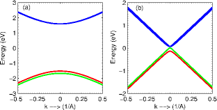
Figure 1: The dispersion of mono-layer MoS₂ under off-resonant light condition. The sub-figure on the left (right) plots the band dispersion around the $K(K^{\prime})$ point.

We have until now obtained the desired form of the Floquet Hamiltonian for a mono-layer TMDC; for the next stage of calculations involving SHC, the Fermi level is positioned to the top of the valence bands such that the conduction bands are devoid of carriers. The Kubo expression (for non-interacting particles) for SHC is written using the eigen states and function of the representative Hamiltonian as

$$\sigma_{SH}=-i\dfrac{\hbar\,e}{L^{2}}\sum_{n,n^{{}^{\prime}}}\dfrac{f\left(\varepsilon_{n}\right)-f\left(\varepsilon_{n^{{}^{\prime}}}\right)}{\varepsilon_{n}-\varepsilon_{n^{{}^{\prime}}}}\dfrac{\langle\,n|\,j_{x}^{z}|\,n^{{}^{\prime}}\rangle\langle\,n^{{}^{\prime}}|\,\hat{v}_{y}|\,n\rangle}{\varepsilon_{n}-\varepsilon_{n^{{}^{\prime}}}+i\zeta},$$ (4)

where we choose $|\,n\rangle$ and $|\,n^{{}^{\prime}}\rangle$ to be the valence and conduction eigen functions of the Hamiltonian given in Eq. 3. We also write down the corresponding energy difference for later use using Eq. 2 as $\epsilon_{n^{{}^{\prime}}}-\epsilon_{n}=\sqrt{\left(\Delta-\lambda\right)^{2}+4a^{2}t^{2}k^{2}}$. We explicitly state here that the wave functions are for the $K^{{}^{\prime}}$ valley edge; the choice of the $K^{{}^{\prime}}$ valley edge is dictated by the lower band gap (compared to the $K$ edge) which ensures a higher conductivity response. At the $K^{{}^{\prime}}$ valley, the analytic representation of the wave functions are $\Psi_{VB}=\dfrac{1}{\sqrt{2}}\begin{pmatrix}\eta_{-}e^{-i\theta}\\ -\,\eta_{+}\end{pmatrix}$ and $\Psi_{CB}=\dfrac{1}{\sqrt{2}}\begin{pmatrix}\eta_{+}e^{-i\theta}\\ \,\eta_{-}\end{pmatrix}$ where $\theta=\tan^{-1}k_{y}/k_{x}$ and $\eta_{-}$ and $\eta_{+}$ can be written as

$$\eta_{\pm}=\sqrt{1\pm\dfrac{\Delta-\lambda}{\sqrt{\left(\Delta-\lambda\right)^{2}+\left(2atk\right)^{2}}}}.$$ (5)

Since most TMDC mono-layers have impurities on the surface, their role in adjusting the spin response must be accounted; in this work, disorder is modeled as an effective retarded self-energy within the self-consistent Born approximation (SCBA) that will allow us to estimate the quasi-particle relaxation time and broadening of states. Di Castro and Raimondi (2015) The pair of SCBA equations (for dilute disorder) being:

$$G_{ks}\left(\epsilon\right)=\dfrac{1}{\epsilon-\epsilon_{ks}-\Sigma\left(\epsilon\right)};\Sigma\left(\epsilon\right)=n_{i}v_{i}^{2}\int\,\dfrac{d^{2}k}{4\pi^{2}}G_{ks}\left(\epsilon\right),$$ (6)

where $n_{i}$ and $v_{i}$ denote the density and strength of impurities, respectively and $G_{ks}\left(\epsilon\right)$ is the retarded Green’s function diagonal with respect to the band index s ($\langle\,s|\,G_{k}\left(\epsilon\right)|\,s\rangle=\delta_{ss^{{}^{\prime}}}G_{ks}\left(\epsilon\right)$). The self-energy $\Sigma$ which is also diagonal with respect to the band index s and independent of k in SCBA is averaged over impurity distributions and represented using a Feynman diagram in Fig. 2. The single solid line in Fig. 2 is the unperturbed Green’s function while the combined dashed and solid line serves as the disorder-induced effective self-energy in the lowest approximation.

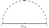
Figure 2: The second order self energy term in the Born approximation after averaging over the impurity distribution. The labels $X$ and $X^{{}^{\prime}}$ denote the placement of two interacting impurities while the dashed line represents their average.

The unperturbed retarded Green’s function for the $2\times 2$ upper block of the Hamiltonian in Eq. 1 is $G_{0,R}=\left(E-H_{\mathcal{F}}^{2\times 2}+i\delta\right)^{-1}$ which when expanded gives

$$G_{0,R}=\dfrac{1}{Det}\begin{pmatrix}E+\dfrac{\Delta}{2}-\lambda+i\delta&-atk\exp\,-i\theta\\ -atk\exp\,i\theta&E-\dfrac{\Delta}{2}+i\delta\end{pmatrix},$$ (7)

where $Det$ is the determinant of the matrix. Inserting $G_{0,R}$ in the self-energy expression (Eq. 6), we recast the diagonal terms to the form $\dfrac{1}{x\pm i0^{+}}$ to separate the real and imaginary parts. The imaginary part of self-energy supplies the inverse of the relaxation time while the real part simply renormalizes the Fermi energy and is absorbed in the chemical potential. Using the standard expression $\dfrac{1}{x\pm i0^{+}}=\mathbb{P}\dfrac{1}{x}\pm i\pi\delta\left(x\right)$, the $\delta\left(\cdot\right)$ functions under integration which lead to the final self-energy imaginary terms are $\delta\left(E+\Delta/2-\lambda-\left(atk\right)^{2}/\left(E-\Delta/2\right)\right)$ and $\delta\left(E-\Delta/2-\left(atk\right)^{2}/\left(E+\Delta/2-\lambda\right)\right)$. Neglecting the $a^{2}t^{2}k^{2}$ term in each of the $\delta\left(\cdot\right)$ functions since we must stay close to the valley edge ($k$ is therefore a small number and the product $atk$ can be neglected), the imaginary part of self-energy is

$$Im\,\Sigma =n_{i}v_{i}^{2}\int\dfrac{d^{2}k}{4\pi^{2}}\biggl{[}\delta\left(E+\Delta/2-\lambda\right)+\delta\left(E-\Delta/2\right)\biggr{]},$$

$$\approx n_{i}v_{i}^{2}\dfrac{1}{2a^{2}t^{2}}\left(|\lambda-\Delta/2|\right).$$ (8)

Notice that $\lambda-\Delta/2$ happens to be the top of the valence band which by assumption is also the position of the Fermi level. The other argument of the $\delta\left(\cdot\right)$ from Eq. 8 is $E=\Delta/2$ which is the base of the conduction band at the valley edges. This energy state is by assumption above the set Fermi level and therefore discarded. Note that the imaginary term in Eq. 4 is $\zeta=\hbar/\tau_{tr}=2Im\Sigma$. The carrier transit time is $\tau_{tr}$.

The spin Hall current that we calculate and has been addressed elsewhere Nomura et al. (2005) in context of a 2DEG with Rashba-coupling is essentially a non-equilibrium situation; an electric field applied along the $\hat{y}-$axis gives rise to an out-of-plane ($\hat{z}$-polarized) non-equilibrium $\hat{x}$-directed spin current. The spin-current operator Murakami (2006) around $K^{{}^{\prime}}\left(\tau=-1\right)$ in this case is $j_{x}^{z}=\dfrac{\hbar}{4}\left\{\hat{v}_{x},\hat{s}_{z}\right\}=-at\sigma_{x}s_{z}/2$, where we have set the electron velocity operator along $\hat{x}-$ and $\hat{y-}$ axes as $\left(-at\hat{\sigma}_{x}/\hbar\right)$ and $\left(at\hat{\sigma}_{y}/\hbar\right)$, respectively. Note that the lattice space operators $\hat{\sigma}_{x,y}$ commute with the Pauli spin operators $\left(\hat{s}_{x},\hat{s}_{y},\hat{s}_{z}\right)$. The matrix elements in Eq. 4, utilizing the eigen states $|\,n\rangle$ and $|\,n^{{}^{\prime}}\rangle$ therefore evaluate to

$$\langle\,n|\,j_{x}^{z}|\,n^{{}^{\prime}}\rangle =\dfrac{at}{2}\left(\cos\theta-i\dfrac{\Delta-\lambda}{\epsilon_{n^{{}^{\prime}}}-\epsilon_{n}}\sin\theta\right),$$ (9)

$$\langle\,n^{{}^{\prime}}|\,\hat{v}_{y}|\,n\rangle =\dfrac{iat}{\hbar}\left(\cos\theta+i\dfrac{\Delta-\lambda}{\epsilon_{n^{{}^{\prime}}}-\epsilon_{n}}\sin\theta\right).$$

Notice that similar spin current operators for polarization and flow along a specific set of axes can also be written; for instance, $j_{x}^{y}=\dfrac{\hbar}{4}\left\{\hat{v}_{x},\hat{s}_{y}\right\}=\hbar\tau\,at\sigma_{x}s_{y}/2$. By a direct substitution of the matrix elements from Eq. 9 followed by expanding the $\sum$ in Eq. 4 (the TMDC mono-layer sample area is assumed to be $\mathcal{A}=L^{2}$) and integrating out the angular part, we obtain the following expression for the SHC in units of $e/8\pi$, the universal SHC. Sinova et al. (2004)

$$\sigma_{xy}^{z}=2a^{2}t^{2}\int_{0}^{k_{c}}\dfrac{\left(\Delta-\lambda\right)^{2}+\left(\epsilon_{n^{{}^{\prime}}}-\epsilon_{n}\right)^{2}}{\left(\epsilon_{n^{{}^{\prime}}}-\epsilon_{n}\right)^{2}\left[\left(\epsilon_{n^{{}^{\prime}}}-\epsilon_{n}\right)^{2}+\zeta^{2}\right]}k\,dk.$$ (10)

The SHC integral in Eq. 10 can be numerically evaluated by choosing a cutoff radius in momentum space around the $K^{{}^{\prime}}$ high-symmetry edge..

For a numerical estimate of $\sigma_{xy}^{z}$, we select band parameters Xiao et al. (2012) for two mono-layer TMDCS, Mo$S_{2}$ and WSe₂. The incident off-resonant illumination with frequencies much higher than the hopping amplitude $t$ must satisfy the inequality López et al. (2015) $\hbar\omega\gg t$; for our case, we select a range of frequencies that lie within $5t\leq\hbar\omega\leq 10t$. Additionally, to evaluate the retarded self-energy, the impurity concentration was set to $2.5\times 10^{10}\,cm^{-2}$ and the impurity potential was assigned the value of $0.1\,keV\,\AA^{2}$. Adam et al. (2009) These numbers using Eq. 8 yields a self-energy (imaginary contribution) approximately equal to $4.6\,meV$ and $8.0\,meV$ for WSe₂ and MoS₂, respectively. Lastly, we choose the cutoff radius as $k_{c}=1.0\,1/\AA$. The incident energy of the beam ($evA$) for all calculations has been held constant at $2.0\,eV$ and as noted before is a tunable quantity via the intensity $I$. Inserting these numbers in Eq. 10 and carrying out a numerical integration, the calculated $\sigma_{xy}^{z}$ as a function of incident light energy is plotted in Fig. 3.

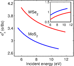
Figure 3: The SHC of mono-layer MoS₂ and WSe₂ samples irradiated under off-resonant conditions for various incident energies at constant intensity. The higher spin-orbit coupling in WSe₂ results in an enhanced SHC. The inset shows the variation in band gap at the $K^{{}^{\prime}}$ edge of the mono-layer.

The SHC from Fig. 3 is a fraction of the universal spin Hall constant of $e/8\pi$ and shows a declining trend as the frequency increases which is easily explained by resorting to the Floquet dependence of the band gap. The band gap reduction for a constant energy beam is lower for a higher frequency which essentially means a higher effective band gap at $K^{{}^{\prime}}$ edge. The inset in Fig. 3 supports this reasoning. While we have focused on band gap alterations through frequency modulation at constant intensity, it is also possible to arrive at an identical outcome by adopting the opposite. As a concrete example, the band gap at the $K^{{}^{\prime}}$ edge under off-resonant conditions for two equal energy ($\hbar\omega=10t=11\,eV$) light beams whose incident energy is set to $2.0\,eV$ and $3.0\,eV$, the overall effective band gap is $0.854\,eV$ and $2.314\,eV$, respectively. The corresponding SHC, as reasoned for the case of higher frequency therefore drops with an increase in the incident energy.

We want to point out that although the TMDC mono-layer is considered pristine, edge defects and corrugations in a real sample can quantitatively alter the final SHC through a reduction in overall charge mobility (we ignore any possible broadening of the local density of states). Further, the SHC is theoretically temperature dependent, this dependence arises from the change of mobility and carrier velocity. However, for device operation and measurements performed in a small range of ambient conditions (room temperature), we should expect a minimal shift in mobility values for any discernible changes to spin conductivity.

In conclusion, we have shown that the SHC in mono-layer TMDCs under off-resonant conditions is tunable via the intensity and frequency of incident light. The procedure can be easily extended to similar material systems that hosts massive Dirac fermions including ultra-thin topological insulator films and other emerging 2D materials such as black phosphorus.

This work was supported in part by the U.S. Army Research Laboratory through the MSME Collaborative Research Alliance.

References

- Wang et al. (2012) Q. H. Wang, K. Kalantar-Zadeh, A. Kis, J. N. Coleman, and M. S. Strano, Nature nanotechnology 7, 699 (2012).
- Huang et al. (2013) X. Huang, Z. Zeng, and H. Zhang, Chemical Society Reviews 42, 1934 (2013).
- Lee et al. (2013) G. Lee, Y. Yu, X. Cui, N. Petrone, C.-H. Lee, M. S. Choi, D. Lee, C. Lee, W. J. Yoo, K. Watanabe, et al., ACS nano 7, 7931 (2013).
- Xiao et al. (2012) D. Xiao, G.-B. Liu, W. Feng, X. Xu, and W. Yao, Physical Review Letters 108, 196802 (2012).
- Tahir et al. (2014) M. Tahir, A. Manchon, and U. Schwingenschlögl, Physical Review B 90, 125438 (2014).
- López et al. (2015) A. López, A. Scholz, B. Santos, and J. Schliemann, Physical Review B 91, 125105 (2015).
- Hatami et al. (2014) H. Hatami, T. Kernreiter, and U. Zülicke, Physical Review B 90, 045412 (2014).
- Yao et al. (2007) W. Yao, A. MacDonald, and Q. Niu, Physical review letters 99, 047401 (2007).
- Kitagawa et al. (2011) T. Kitagawa, T. Oka, A. Brataas, L. Fu, and E. Demler, Physical Review B 84, 235108 (2011).
- Zhu et al. (2014) B. Zhu, H. Zeng, J. Dai, and X. Cui, Advanced Materials 26, 5504 (2014).
- Konabe and Yamamoto (2014) S. Konabe and T. Yamamoto, Physical Review B 90, 075430 (2014).
- Cayssol et al. (2013) J. Cayssol, B. Dóra, F. Simon, and R. Moessner, physica status solidi (RRL)-Rapid Research Letters 7, 101 (2013).
- Tannor (2007) D. J. Tannor, Introduction to quantum mechanics: A time-dependent perspective (University Science Books, 2007).
- Zhai and Jin (2014) X. Zhai and G. Jin, Physical Review B 89, 235416 (2014).
- Di Castro and Raimondi (2015) C. Di Castro and R. Raimondi, Statistical Condensed Matter Physics (Cambridge University Press, 2015).
- Nomura et al. (2005) K. Nomura, J. Sinova, T. Jungwirth, Q. Niu, and A. MacDonald, Physical Review B 71, 041304 (2005).
- Murakami (2006) S. Murakami, in Advances in Solid State Physics (Springer, 2006), pp. 197–209.
- Sinova et al. (2004) J. Sinova, D. Culcer, Q. Niu, N. Sinitsyn, T. Jungwirth, and A. MacDonald, Physical Review Letters 92, 126603 (2004).
- Adam et al. (2009) S. Adam, E. Hwang, E. Rossi, and S. D. Sarma, Solid State Communications 149, 1072 (2009).