Departure of high temperature iron lines from the equilibrium state in flaring solar plasmas

Abstract

The aim of this study is to clarify if the assumption of ionization equilibrium and a Maxwellian electron energy distribution is valid in flaring solar plasmas. We analyse the 2014 December 20 X1.8 flare, in which the Fe xxi 187 Å, Fe xxii 253 Å, Fe xxiii 263 Å and Fe xxiv 255 Å emission lines were simultaneously observed by the EUV Imaging Spectrometer onboard the Hinode satellite. Intensity ratios among these high temperature Fe lines are compared and departures from isothermal conditions and ionization equilibrium examined. Temperatures derived from intensity ratios involving these four lines show significant discrepancies at the flare footpoints in the impulsive phase, and at the looptop in the gradual phase. Among these, the temperature derived from the Fe xxii/Fe xxiv intensity ratio is the lowest, which cannot be explained if we assume a Maxwellian electron distribution and ionization equilibrium, even in the case of a multi-thermal structure. This result suggests that the assumption of ionization equilibrium and/or a Maxwellian electron energy distribution can be violated in evaporating solar plasma around 10 MK.

1 Introduction

Solar flares are one of the most important phenomena to investigate the processes of energy development and its release in the solar atmosphere. Magnetic reconnection (Shibata & Magara, 2011) is now widely accepted as the energy release mechanism of solar flares both theoretically (e.g. Carmichael, 1964) and observationally (e.g. Tsuneta et al., 1992). However, the rate of energy transformation from magnetic into thermal, nonthermal and/or kinetic energy is still unknown. The derivation of physical parameters for the energetics is crucial for answering this question.

Spectroscopic observations are a powerful tool for diagnosing the physical parameters of the plasma. Temperature and density diagnostics are, in most instances, based on the assumption of ionization equilibrium and a Maxwellian electron energy distribution. However, soft X-ray spectroscopic observations indicated that the ion temperatures derived from satellite transitions or line widths are sometimes lower than the electron temperatures during early flare stages (Doschek & Tanaka, 1987; Kato et al., 1998). This indicates a thermal decoupling of these species, and the long collisional timescales have implications for other collisionally-dominated processes such as the ionization state and the electron distribution. Emissivities under non-equilibrium ionization conditions due to heating and cooling processes during flares have also been investigated via numerical simulations (Bradshaw & Mason, 2003; Reale & Orlando, 2008). The timescale to achieve ionization equilibrium depends on the electron density (Bradshaw, 2009; Smith & Hughes, 2010), and the non-equilibrium ionization state may not be negligible in both the energy release site (Imada et al., 2011) and the evaporated plasma (Bradshaw & Cargill, 2006).

Non-Maxwellian distributions have been discussed primarily in the context of temperature diagnostics using soft X-ray satellite lines that are not affected by ionization processes (Gabriel & Phillips, 1979; Seely et al., 1987). Such non-Maxwellians have been employed as diagnostics of nonthermal electrons, and UV emission lines have also been examined to assess if they allow the detection of nonthermal electrons (Pinfield et al., 1999; Feldman et al., 2008; Dzifčáková & Kulinová, 2010; Dudík et al., 2014).

Here we examine the interrelationship of the intensities of high temperature lines that may be strongly affected by non-equilibrium ionization both spatially and temporally. We investigate if the assumption of ionization equilibrium and a Maxwellian electron distribution is valid in 10⁷ K solar plasma during an X-class flare, using spectra from the EUV Imaging Spectrometer (EIS; Culhane et al., 2007) onboard the Hinode satellite (Kosugi et al., 2007). Our paper is laid out as follows. In Section 2 we investigate the characteristics of high temperature Fe lines observed by EIS in terms of temperature and density under Maxwellian distribution and ionization equilibrium conditions, while in Section 3 we analyse an X-class flare and show results of intensity interrelationships for the Fe lines. Finally in Section 4 we discuss possible departures from thermal equilibrium and present our conclusions.

2 Characteristics of flare lines in the EIS observation

2.1 Fe XXI, Fe XXII, Fe XXIII and Fe XXIV

We first briefly examine the characteristics of high temperature Fe lines we have selected. CHIANTI version 8.0.1 (Dere et al., 1997; Del Zanna et al., 2015) was used to calculate the line intensities, and we adopted the coronal abundances of Schmelz et al. (2012) and ionization fractions of Bryans et al. (2009), with a Maxwellian distribution in the ionization equilibrium.

Under the coronal approximation, most electrons are in the ground state and excitation is due to electron collisions. Thus, the line intensity depends on the electron collisional rate and the population of the upper level of the relevant transition along the line-of-sight. Hence if we derive the intensity ratio of two lines with significantly different excitation energies, this ratio will depend on both the electron energy distribution and the level populations. The electron energy distribution is, in most cases, assumed to be Maxwellian, i.e. a function of temperature. In addition, if we assume the plasma is in ionization equilibrium, the ratio of the line intensities is determined by temperature and column density. Figure 1(a) shows the contribution functions of the lines considered here under the assumption of a Maxwellian distribution and ionization equilibrium. These lines are formed at similar temperatures around 10 MK. We also show the temperature and density dependence of intensity ratios involving these lines in Figure 1(b) and (c), respectively. The temperature sensitivity is strong, while there is only a weak dependence on density. Therefore, if a hot plasma is assumed to be isothermal and in ionization equilibrium, the electron distribution is determined by the intensity ratios among pairs of these lines. However, if either assumption of an isothermal plasma or ionization equilibrium is violated, the relationships in the figures no longer hold. In a flaring region, Fe xxii 253 Å is unblended, and Fe xxiii 263 Å and Fe xxiv 255 Å only have some minor blended lines, while Fe xxi 187 Å is completely blended with Ar xiv. There is another Ar xiv line at 194 Å in the EIS observation, although the ratio of these shows a density sensitivity around 10¹⁰ to 10¹² cm^-3. Since there is uncertainty in the plasma densities, it is difficult to deblend the Fe xxi + Ar xiv 187 Å feature, especially in a flaring region where the coronal density for a $10^{7}$ K plasma is around $10^{10}$ to $10^{12}$ cm^-3 (Doschek et al., 1981; Mason et al., 1984; Milligan et al., 2012).

Figure 1: Density and temperature dependence from CHIANTI of the solar emission lines considered in the present paper. (a) Contribution function of Fe xxi+Ar xiv 187 Å (dark-blue dotted line), Fe xxi 187 Å (light-blue solid line), Fe xxii 253 Å (green dashed line), Fe xxiii 263 Å (red dot-dashed line), Fe xxiv 255 Å (black solid line). (b) Temperature dependence of intensity ratios relative to the Fe xxiv 255 Å line, with same line and colour coding as in (a). (c) Density dependence of intensity ratios relative to the Fe xxiv 255 Å line, with the same line and colour coding as in (a). Thick lines show intensity ratios at an electron temperature of log T_e = 7.2, while thin lines show values for log T_e = 7.0. (d) Density dependence of the Ar xiv 187 Å/194 Å intensity ratio at log T_e = 6.6 (black solid line), 7.0 (red dotted line) and 7.2 (blue solid line).

2.2 Multi-thermal structures

A multi-thermal structure along the line-of-sight will result in a departure from the isothermal assumption in the optically thin solar corona. This has been discussed in earlier studies using differential emission measure analyses (Graham et al., 2013; Fletcher et al., 2013). Here we examine intensity ratios involving high temperature Fe lines in a multi-thermal structure in which each layer is assumed to have a Maxwellian distribution in ionization equilibrium. Henceforth we denote the intensities of Fe xxi 187 Å, Fe xxii 253 Å, Fe xxiii 263 Å, and Fe xxiv 255 Å as $I_{21}$, $I_{22}$, $I_{23}$ and $I_{24}$, respectively. To simplify the analysis, we assume that the temperature structure consists of two components at log T_e = 6.9 and 7.2 close to the peaks of the contribution functions of Fe xxi to Fe xxiv, and we vary the fraction of emission measures between the two temperatures. Figure 2(a) and (b) show ratio-ratio plots involving the intensities of the four Fe lines, for different relative fractions of the emission measures. The total overall intensity arises from regions which have the larger fluxes in the lower ionized species, regardless of the relative fractions of the emission measures. To examine the relationships among the intensities simultaneously, we also show ratio-ratio plots for temperatures from the line ratios in Figure 2(c). The figure suggests that, in the case of the two-thermal model log T_e = 6.9 and 7.2, $T(I_{21}/I_{24})<T(I_{22}/I_{24})<T(I_{23}/I_{24})$ is always valid. This result comes from the curvature of the iso-thermal relationship among the line ratios shown in Figure 1(b). Hence, even if we examine the relationships at different temperatures, $T(I_{21}/I_{24})<T(I_{22}/I_{24})<T(I_{23}/I_{24})$ is always valid under conditions of ionization equilibrium and a Maxwellian distribution.

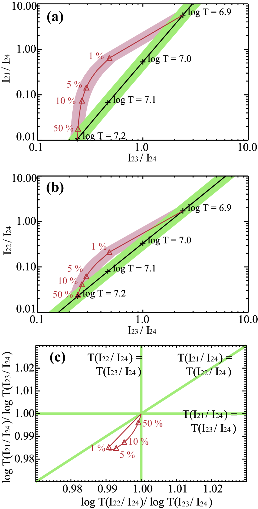
Figure 2: Ratio-ratio plots calculated with CHIANTI of (a) $I_{21}/I_{24}$ versus $I_{23}/I_{24}$, (b) $I_{22}/I_{24}$ versus $I_{23}/I_{24}$, (c) a ratio-ratio plot of $T(I_{21}/I_{24})/T(I_{23}/I_{24})$ versus $T(I_{22}/I_{24})/T(I_{23}/I_{24})$, where the ratios are defined in Section 2.2. In (a) and (b), black lines show the isothermal state, while green-filled regions show errors in intensity ratios under the isothermal state, estimated by assuming an uncertainty of $\pm$10% in the adopted atomic data. Red lines in (a), (b) and (c) indicate two-temperature models along the line-of-sight with temperatures of log T_e = 6.9 and 7.2. Triangles mark the fractions of the emission measure at log T_e = 6.9 of 1, 5, 10 and 50%. The red-filled regions in (a) and (b) show errors in the intensity ratios under two-temperature conditions, once again estimated by adopting a $\pm$10% uncertainty in the atomic data.

3 Data analysis and results

3.1 Overview of observations

Our observational dataset consists of an X1.8 class flare, which occurred in active region NOAA12242 on 2014 December 20. The GOES soft X-ray flux reached its maximum at 00:28 UT, and the location of the active region was S19W29 in the solar coordinate system. This flare was simultaneously observed by Hinode/EIS, the Atmospheric Imaging Assembly (AIA; Lemen et al., 2012) onboard the Solar Dynamics Observatory (SDO; Pesnell et al., 2012), and the Nobeyama Radio Polarimeter (NoRP; Torii et al., 1979; Nakajima et al., 1985) from the impulsive phase to the decay phase. NoRP observed microwave emission, which during solar flares mainly originates from semi-relativistic electrons in a flare loop via gyro-synchrotron emission. Hence, we can determine the time when the nonthermal electrons were created and the evaporated plasma filled the loop.

EIS observations were performed in a slit scanning mode with a 2^′′ wide slit and 3^′′ step size, and at a raster cadence of 534 s. The exposure time was 5 s, and the number of steps was 80 for one raster. Window height along the slit was 304 pixels with spatial sampling of 1^′′ pixel^-1. The field-of-view of the spatial range was therefore 304^′′ along the slit (north-south) and 240^′′ along the raster (west to east), centred at (445^′′, –263^′′). EIS selected 15 spectral windows during these observations, and in our study we focused on the Fe xxi 187 Å, Fe xxii 253 Å, Fe xxiii 263 Å and Fe xxiv 255 Å lines, whose typical formation temperatures are about 10 MK.

3.2 Calibration of spectral data

We calibrated intensities of the EIS data by the following procedures. First, we ran eis_prep to subtract dark current, remove hot/warm pixels by cosmic rays, and calibrate the photometry using the laboratory data (Lang et al., 2006). Through this process we obtained level-1 data. Second, we ran eis_wave_corr_hk to correct the spatial offset in wavelength due to the orbital variation of the satellite (Kamio et al., 2010). Third, we corrected the post-flight sensitivity of the absolute calibration by using the eis_recalibrate_intensity function (Warren et al., 2014). Fourth, we co-aligned spatial pixels along the wavelength direction by using eis_ccd_offset (Young et al., 2009). The instrumental line FWHM for a slit width of 2^′′ in EIS is typically 62 mÅ (Brown et al., 2008), which the thermal FWHM is given by $2\sqrt{\ln 2(kT/M_{i})}$ in velocity unit, where $k$ is Boltzmann’s constant, $T$ the temperature, and $M_{i}$ the mass of the ion. In the case of these Fe lines at their formation temperatures ($\sim 10^{7}$ K), this yields thermal FWHMs of 91 km s^-1, corresponding to 57 mÅ at 187 Å and 80 mÅ at 263 Å. Therefore, we cannot resolve lines within about $\pm 50$ mÅ of the high temperature Fe transitions. Also, during a flare these lines can be both red- and blue-shifted, with Doppler velocities of typically about 30 and 200 km s^-1, respectively (Milligan & Dennis, 2009; Hara et al., 2011), corresponding to 125–176 mÅ for these lines. Since Fe xxi and Ar xiv at 187 Å are completely blended as discussed previously, we estimated an upper limit for the Fe xxi intensity by determining a lower limit for Ar xiv, using the measured Ar xiv 194 Å flux and the theoretical Ar xiv 187 Å/194 Å ratio from CHIANTI.

To determine the continuum level accurately, we fitted lines in the same window simultaneously with a multi-Gaussian function using the MPFIT procedure (Markwardt, 2009; Moré, 1978). Particularly in flare kernels, each line may have multiple components in one pixel (Asai et al., 2008), so we used a two-Gaussian function for each high-temperature Fe line to measure accurate intensities. Pixels in which intensities were less than 2$\times 10^{3}$ erg cm^-2 s^-1Å^-1 sr^-1 were removed from the fitting. The number of Gaussian functions was six for the 188 Å window, four for 253 Å, five for both 263 Å and 255 Å, and seven for 194 Å. The Fe xii, Fe xi and O iv ions in the 188, 188 and 253 Å windows, respectively, each emit two lines in the same window. We assumed that each line pair has the same Doppler velocity and a fixed intensity ratio determined from CHIANTI. There were several hot/warm pixels that were not flagged in the eis_prep procedure, and we removed these from the fitting manually.

We determined the intensity of each line by integrating the Gaussian functions centered from –74 to +100 km s^-1 around each high temperature Fe line, corresponding to –46 to +62 mÅ at 187 Å and –65 to +88 mÅ at 263 Å. This velocity limit is determined by the edge of the wavelength window of 187 Å in the EIS data. Spatial pixels included in this analysis were limited by the following criteria: (i) the continuum intensity obtained by the fitting has a positive value in all five wavelength windows; (ii) the reduced $\chi^{2}$ of the fitting for Fe xxii, Fe xxiii and Fe xxiv is less than 3; (iii) we only include the field-of-view spanning 350^′′ to 550^′′ in the east-west axis and –310^′′ to –260^′′ in the north-south axis, i.e. only regions around the flare. As a result, 633 sets of spectra were obtained. Examples of our fitting procedures are shown in Figure 3.

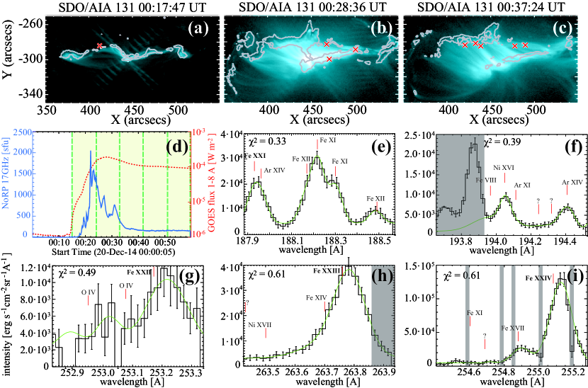
Figure 3: AIA 131 Å images of the 2014 December 20 solar flare during raster periods of (a) 00:15–00:24 UT, (b) 00:24–00:33 UT, and (c) 00:33–00:41, with the time when each image was observed at the top of the panel. The red crosses indicate the position where the temperature shows a departure from isothermal. Grey contours show the AIA 1700 Å image observed 6 s before each AIA 131 Å one. (d) Lightcurves of the 17 GHz (blue thick line) and 1–8 Å (red dotted line) emission observed by NoRP and GOES, respectively. Sets of raster exposures with EIS are shown as green dashed lines, and yellow-filled regions indicate when EIS flare data are available. (e)–(i) Example spectra where the intensity relationship between $T(I_{22}/I_{24})$ and $T(I_{23}/I_{24})$ showed significant departures from isothermal. Green solid curves show the best-fit function of the multi-Gaussian, and the $\chi^{2}$ value for each is given in the top-left portion of each plot. Emission lines included in the multi-Gaussian fitting are labelled, with high temperature Fe lines indicated with a bold font. Grey-filled regions show wavelengths we removed manually from the fitting due to warm pixels.

3.3 Intensity ratios

We calculated intensities of the Fe lines for a Maxwellian distribution and ionization equilibrium by changing temperature in CHIANTI. The grid points of temperature were from log T_e = 6.6 to 7.6 in steps of 0.1 dex, with intermediate values interpolated by a spline function. Ratios were calculated at a single density of N_e = 10¹⁰ cm^-3, as their dependence on density is small, changing by less than 6% for densities up to 10¹¹ cm^-3, smaller than the expected accuracy of the calculations given errors in the atomic data of 10% (Chidichimo et al., 2005; Del Zanna et al., 2005). If the actual density is greater than 10¹¹ cm^-3, the line that is most affected by high density is Fe xxi 187 Å, and the derived temperature from this will be overestimated. At N_e = 10¹¹ cm^-3, the overestimation of the logarithmic temperature derived from $I_{21}/I_{24}$ increases with T_e, but is only 0.01 and 0.02 dex higher at log T_e = 6.9 and 7.2, respectively.

As discussed in Section 2.2, if the plasma is Maxwellian and in ionization equilibrium, the temperatures derived from line ratios should show the relationship $T(I_{21}/I_{24})<T(I_{22}/I_{24})<T(I_{23}/I_{24})$. However, if the plasma does not obey these conditions, the derived temperatures may not follow this relationship. Figure 4(a) and (b) show the ratio-ratio relationships for the observations during 00:15–00:41 UT, with significant data points that lie more than 1 $\sigma$ from the equilibrium in the $I_{22}/I_{24}$ – $I_{23}/I_{24}$ relation emphasised. As noted previously, the values of $I_{21}/I_{24}$ are upper limits. The corresponding observational points in the ratio-ratio diagram are displayed in Figure 4 (c). We obtain two results from these plots. First, 9 out of the 633 pixels in the flaring region show significant departure from the isothermal and ionization equilibrium conditions in the $I_{22}/I_{24}$ – $I_{23}/I_{24}$ relation. Second, all pixels that show such a significant departure have a temperature relationship of $T(I_{22}/I_{24})<T(I_{23}/I_{24})$ and $T(I_{22}/I_{24})<T(I_{21}/I_{24})$. The mean value of $\log T(I_{22}/I_{24})/\log T(I_{23}/I_{24})$ is 0.985$\pm$0.001, while the lower limit of the mean value of $\log T(I_{21}/I_{24})/\log T(I_{23}/I_{24})$ is 0.989$\pm$0.001 among intensity ratios that show significant departures in the rasters. From Figure 4, the highest temperature that shows a departure is log T_e = 7.2, so that the above temperature relationship does not change even considering the case of an electron density of 10¹² cm^-3.

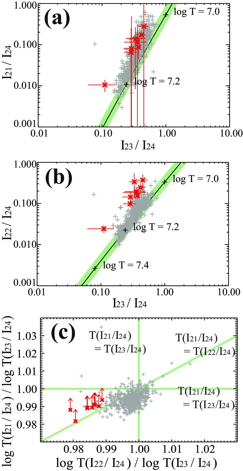
Figure 4: (a) and (b) show ratio-ratio plots calculated with CHIANTI for $I_{22}/I_{24}$ versus $I_{23}/I_{24}$ and $I_{21}/I_{24}$ versus $I_{23}/I_{24}$, respectively. Black lines show the ratio-ratio relationship under Maxwellian and ionization equilibrium conditions. Green-filled regions show the error in the equilibrium intensity ratio assuming a $\pm$10% error in the adopted atomic data. Grey crosses show observed intensity ratios derived from pixels with well-fitted profiles ($\chi^{2}<3$). Red crosses with error bars are measured intensity ratios that are more than 1-$\sigma$ from the equilibrium state. (c) shows the temperature relationship among $T(I_{21}/I_{24})$, $T(I_{22}/I_{24})$ and $T(I_{23}/I_{24})$ derived from the observed intensity ratios. Red crosses are data points that are more than 1-$\sigma$ from the equilibrium state between $T(I_{22}/I_{24})$ and $T(I_{23}/I_{24})$. Green lines show the relationships $T(I_{21}/I_{24})=T(I_{22}/I_{24})$, $T(I_{21}/I_{24})=T(I_{23}/I_{24})$, and $T(I_{22}/I_{24})=T(I_{23}/I_{24})$ under the isothermal assumption.

To further assess our results, we investigate in Figure 3(a), (b), and (c) the spatial position where the intensity ratio shows a significant departure from equilibrium. In the figures, AIA 1700 Å images are also plotted as a reference for the chromospheric flare footpoints. Comparing with the timing of the impulsive phase shown in Figure 3(d), the significant departure appears at the footpoint in the impulsive phase, while in the gradual phase the departure appears mainly in the looptop. We plot in Figure3(e)–(i) one set of spectra from the pixel which shows a significant departure. All of the spectra are well fitted using the multi-Gaussian function, producing maximum errors of $\chi^{2}<0.61$.

4 Discussion and summary

We have examined the intensity relationships among Fe lines observed in an X-class flare. For 9 out of 633 pixels, the temperatures derived from the intensities show departure from the isothermal and ionization equilibrium conditions. Temperature dependencies of $T(I_{22}/I_{24})<T(I_{23}/I_{24})$ and $T(I_{22}/I_{24})<T(I_{21}/I_{24})$ were found, suggesting that the assumption of a Maxwellian electron distribution and/or ionization equilibrium is violated. Pixels where the intensities showed a significant departure from the isothermal condition in the $I_{22}/I_{24}$ - $I_{23}/I_{24}$ relation are located at the footpoint in the impulsive phase, and looptop in the gradual phase.

The number of pixels that show departures from isothermal and ionization equilibrium conditions is as small as 1.4% compared to that of valid pixels in the entire flaring region. Therefore, we could conclude that ionization equilibrium is valid in most cases within the timescale of the EIS exposures. However, all pixels that show a departure from thermal equilibrium have the same temperature relationship, which implies the same physical processes are occurring in the region. The number of pixels is highly influenced by the timing of the slit exposure, errors in the observations, and the validity of the assumption in the models. Nevertheless, we can also conclude that the assumption of isothermal and ionization equilibrium conditions is not valid in some cases. Significant departures from this assumption can be explained by the following. The departure from equilibrium conditions appeared at the footpoint in the impulsive phase and looptop in the late gradual phase, suggesting that the departure arises along the path of evaporation. At the footpoints of the impulsive phase, the non-thermal tail under a non-Maxwellian electron distribution would favor the creation of more strongly ionized species, as well as rapid heating due to the evaporated plasmas. The apparent temperatures among these line ratios are always overestimated under non-equilibrium ionization and a non-Maxwellian distribution. Even examining pure non-equilibrium ionization, it takes about 10${}^{3}(10^{9}/N_{e})^{-1}$ s to reach ionization equilibrium for Fe xxiv (Bradshaw, 2009; Imada et al., 2011). Since Fe xxi starts to ionize earliest among these species, $T(I_{21}/I_{24})$ is higher than $T(I_{22}/I_{24})$ and $T(I_{23}/I_{24})$ in the heating phase. This may explain the observed temperature relationships if $T(I_{21}/I_{24})>T(I_{23}/I_{24})$ is valid, although we cannot confirm this since we only provide a lower limit to $T(I_{21}/I_{24})$. If $T(I_{21}/I_{24})>T(I_{23}/I_{24})$ is not valid, a non-Maxwellian electron distribution may couple with a non-equilibrium ionization in a multi-thermal structure, and we would need detailed numerical simulations to understand this fully. On the other hand, at the looptop in the gradual phase, the evaporated plasmas fill the flare loop and radiative cooling dominates in the temperature evolution. More highly ionized species are over populated, and the temperature relationship is $T(I_{21}/I_{24})<T(I_{22}/I_{24})<T(I_{23}/I_{24})$, which cannot be distinguished from the relationship under ionization equilibrium, and multi-thermal structures cannot explain the observed result. An explanation for the observed result would be coupling of the high energy tail in the electron distribution, i.e., a non-Maxwellian distribution with non-equilibrium ionization. However, it is difficult to solve the inverse problem, (i.e., determine the degree of non-equilibrium ionisation or extent of non-thermal structures) solely from high-temperature line ratios. Further studies of combined models for the simultaneous evolution of electron distribution and non-equilibrium ionization, and employing better sensitivity with higher cadence observations, are needed to explain this phenomenon.

References

- Asai et al. (2008) Asai, A., Hara, H., Watanabe, T., et al. 2008, ApJ, 685, 622
- Bradshaw (2009) Bradshaw, S. J. 2009, A&A, 502, 409
- Bradshaw & Cargill (2006) Bradshaw, S. J., & Cargill, P. J. 2006, A&A, 458, 987
- Bradshaw & Mason (2003) Bradshaw, S. J., & Mason, H. E. 2003, A&A, 401, 699
- Brown et al. (2008) Brown, C. M., Feldman, U., Seely, J. F., Korendyke, C. M., & Hara, H. 2008, ApJS, 176, 511
- Bryans et al. (2009) Bryans, P., Landi, E., & Savin, D. W. 2009, ApJ, 691, 1540
- Carmichael (1964) Carmichael, H. 1964, NASA Special Publication, 50, 451
- Chidichimo et al. (2005) Chidichimo, M. C., Del Zanna, G., Mason, H. E., et al. 2005, A&A, 430, 331
- Culhane et al. (2007) Culhane, J. L., Harra, L. K., James, A. M., et al. 2007, Sol. Phys., 243, 19
- Del Zanna et al. (2005) Del Zanna, G., Chidichimo, M. C., & Mason, H. E. 2005, A&A, 432, 1137
- Del Zanna et al. (2015) Del Zanna, G., Dere, K. P., Young, P. R., Landi, E., & Mason, H. E. 2015, A&A, 582, A56
- Dere et al. (1997) Dere, K. P., Landi, E., Mason, H. E., Monsignori Fossi, B. C., & Young, P. R. 1997, A&AS, 125, 149
- Doschek et al. (1981) Doschek, G. A., Feldman, U., Landecker, P. B., & McKenzie, D. L. 1981, ApJ, 249, 372
- Doschek & Tanaka (1987) Doschek, G. A., & Tanaka, K. 1987, ApJ, 323, 799
- Dudík et al. (2014) Dudík, J., Del Zanna, G., Mason, H. E., & Dzifčáková, E. 2014, A&A, 570, A124
- Dzifčáková & Kulinová (2010) Dzifčáková, E., & Kulinová, A. 2010, Sol. Phys., 263, 25
- Feldman et al. (2008) Feldman, U., Ralchenko, Y., & Landi, E. 2008, ApJ, 684, 707
- Fletcher et al. (2013) Fletcher, L., Hannah, I. G., Hudson, H. S., & Innes, D. E. 2013, ApJ, 771, 104
- Gabriel & Phillips (1979) Gabriel, A. H., & Phillips, K. J. H. 1979, MNRAS, 189, 319
- Graham et al. (2013) Graham, D. R., Hannah, I. G., Fletcher, L., & Milligan, R. O. 2013, ApJ, 767, 83
- Hara et al. (2011) Hara, H., Watanabe, T., Harra, L. K., Culhane, J. L., & Young, P. R. 2011, ApJ, 741, 107
- Imada et al. (2011) Imada, S., Murakami, I., Watanabe, T., Hara, H., & Shimizu, T. 2011, ApJ, 742, 70
- Kamio et al. (2010) Kamio, S., Hara, H., Watanabe, T., Fredvik, T., & Hansteen, V. H. 2010, Sol. Phys., 266, 209
- Kato et al. (1998) Kato, T., Fujiwara, T., & Hanaoka, Y. 1998, ApJ, 492, 822
- Kosugi et al. (2007) Kosugi, T., Matsuzaki, K., Sakao, T., et al. 2007, Sol. Phys., 243, 3
- Lang et al. (2006) Lang, J., Kent, B. J., Paustian, W., et al. 2006, Appl. Opt., 45, 8689
- Lemen et al. (2012) Lemen, J. R., Title, A. M., Akin, D. J., et al. 2012, Sol. Phys., 275, 17
- Markwardt (2009) Markwardt, C. B. 2009, in Astronomical Society of the Pacific Conference Series, Vol. 411, Astronomical Data Analysis Software and Systems XVIII, ed. D. A. Bohlender, D. Durand, & P. Dowler, 251
- Mason et al. (1984) Mason, H. E., Bhatia, A. K., Neupert, W. M., Swartz, M., & Kastner, S. O. 1984, Sol. Phys., 92, 199
- Milligan & Dennis (2009) Milligan, R. O., & Dennis, B. R. 2009, ApJ, 699, 968
- Milligan et al. (2012) Milligan, R. O., Kennedy, M. B., Mathioudakis, M., & Keenan, F. P. 2012, ApJ, 755, L16
- Moré (1978) Moré, J. J. 1978, in Lecture Notes in Mathematics, Vol. 630, Numerical Analysis, ed. G. Watson (Springer Berlin Heidelberg), 105–116
- Nakajima et al. (1985) Nakajima, H., Sekiguchi, H., Sawa, M., Kai, K., & Kawashima, S. 1985, PASJ, 37, 163
- Pesnell et al. (2012) Pesnell, W. D., Thompson, B. J., & Chamberlin, P. C. 2012, Sol. Phys., 275, 3
- Pinfield et al. (1999) Pinfield, D. J., Keenan, F. P., Mathioudakis, M., et al. 1999, ApJ, 527, 1000
- Reale & Orlando (2008) Reale, F., & Orlando, S. 2008, ApJ, 684, 715
- Schmelz et al. (2012) Schmelz, J. T., Reames, D. V., von Steiger, R., & Basu, S. 2012, ApJ, 755, 33
- Seely et al. (1987) Seely, J. F., Feldman, U., & Doschek, G. A. 1987, ApJ, 319, 541
- Shibata & Magara (2011) Shibata, K., & Magara, T. 2011, Living Reviews in Solar Physics, 8, doi:10.12942/lrsp-2011-6
- Smith & Hughes (2010) Smith, R. K., & Hughes, J. P. 2010, ApJ, 718, 583
- Torii et al. (1979) Torii, C., Tsukiji, Y., Kobayashi, S., et al. 1979, Proceedings of the Research Institute of Atmospherics, Nagoya University, 26, 129
- Tsuneta et al. (1992) Tsuneta, S., Hara, H., Shimizu, T., et al. 1992, PASJ, 44, L63
- Warren et al. (2014) Warren, H. P., Ugarte-Urra, I., & Landi, E. 2014, ApJS, 213, 11
- Young et al. (2009) Young, P. R., Watanabe, T., Hara, H., & Mariska, J. T. 2009, A&A, 495, 587