Bayesian Poisson Tucker Decomposition
for Learning the Structure of International Relations

Abstract

We introduce Bayesian Poisson Tucker decomposition (BPTD) for modeling country–country interaction event data. These data consist of interaction events of the form “country $i$ took action $a$ toward country $j$ at time $t$.” BPTD discovers overlapping country–community memberships, including the number of latent communities. In addition, it discovers directed community–community interaction networks that are specific to “topics” of action types and temporal “regimes.” We show that BPTD yields an efficient MCMC inference algorithm and achieves better predictive performance than related models. We also demonstrate that it discovers interpretable latent structure that agrees with our knowledge of international relations.

1 Introduction

Like their inhabitants, countries interact with one another: they consult, negotiate, trade, threaten, and fight. These interactions are seldom uncoordinated. Rather, they are connected by a fabric of overlapping communities, such as security coalitions, treaties, trade cartels, and military alliances. For example, OPEC coordinates the petroleum export policies of its thirteen member countries, LAIA fosters trade among Latin American countries, and NATO guarantees collective defense against attacks by external parties.

A single country can belong to multiple communities, reflecting its different identities. For example, Venezuela—an oil-producing country and a Latin American country—is a member of both OPEC and LAIA. When Venezuela interacts with other countries, it sometimes does so as an OPEC member and sometimes does so as a LAIA member.

Countries engage in both within-community and between-community interactions. For example, when acting as an OPEC member, Venezuela consults with other OPEC countries, but trades with non-OPEC, oil-importing countries. Moreover, although Venezuela engages in between-community interactions when trading as an OPEC member, it engages in within-community interactions when trading as a LAIA member. To understand or predict how countries interact, we must account for their community memberships and how those memberships influence their actions.

In this paper, we take a new approach to learning overlapping communities from interaction events of the form “country $i$ took action $a$ toward country $j$ at time $t$.” A data set of such interaction events can be represented as either 1) a set of event tokens, 2) a tensor of event type counts, or 3) a series of weighted multinetworks. Models that use the token representation naturally yield efficient inference algorithms, models that use the tensor representation exhibit good predictive performance, and models that use the network representation learn latent structure that aligns with well-known concepts such as communities. Previous models of interaction event data have each used a subset of these representations. Our approach—Bayesian Poisson Tucker decomposition (BPTD)—takes advantage of all three.

BPTD builds on the classic Tucker decomposition (Tucker, 1964) to factorize a tensor of event type counts into three factor matrices and a four-dimensional core tensor (section 2). The factor matrices embed countries into communities, action types into “topics,” and time steps into “regimes.” The core tensor interacts communities, topics, and regimes. The country–community factors enable BPTD to learn overlapping community memberships, while the core tensor enables it to learn directed community–community interaction networks specific to topics of action types and temporal regimes. Figure 1 illustrates this structure. BPTD leads to an efficient MCMC inference algorithm (section 4) and achieves better predictive performance than related models (section 6). Finally, BPTD discovers interpretable latent structure that agrees with our knowledge of international relations (section 7).

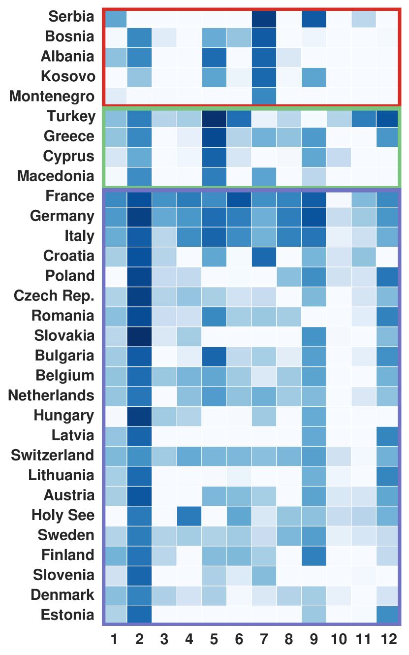
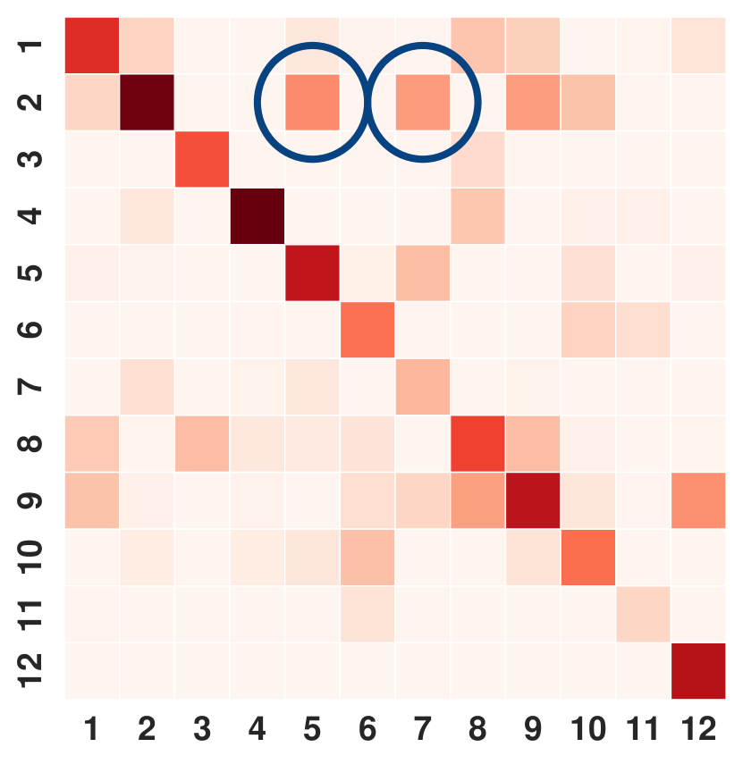
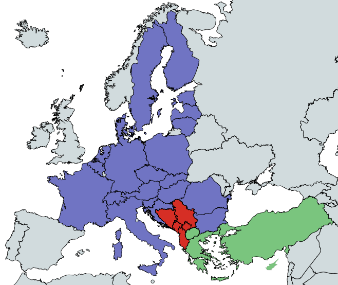
Figure 1: Latent structure learned by BPTD from country–country interaction events between 1995 and 2000. Top right: A community–community interaction network specific to a single topic of action types and temporal regime. The topic places most of its mass on the Intend to Cooperate and Consult actions, so this network represents cooperative community–community interactions. The two strongest between-community interactions (circled) are 2${\xrightarrow{}}$5 and 2${\xrightarrow{}}$7. Left: Each row depicts the overlapping community memberships for a single country. We show only those countries whose strongest community membership is to either community 2, 5, or 7. We ordered the countries accordingly. Countries strongly associated with community 7 are at highlighted in red; countries associated with community 5 are highlighted in green; and countries associated with community 2 are highlighted in purple. Bottom right: Each country is colored according to its strongest community membership. The latent communities have a very strong geographic interpretation.

2 Bayesian Poisson Tucker Decomposition

We can represent a data set of interaction events as a set of $N$ event tokens, where a single token $e_{n}=(i{\xrightarrow{a}}j,t)$ indicates that sender country $i\in[V]$ took action $a\in[A]$ toward receiver country $j\in[V]$ during time step $t\in[T]$. Alternatively, we can aggregate these event tokens into a four-dimensional tensor $\boldsymbol{Y}$, where element $y^{(t)}_{i{\xrightarrow{a}}j}$ is a count of the number of events of type $(i{\xrightarrow{a}}j,t)$. This tensor will be sparse because most event types never actually occur in practice. Finally, we can equivalently view this count tensor as a series of $T$ weighted multinetwork snapshots, where the weight on edge $i{\xrightarrow{a}}j$ in the $t^{\textrm{th}}$ snapshot is $y^{(t)}_{i{\xrightarrow{a}}j}$.

BPTD models each element of count tensor $\boldsymbol{Y}$ as

$$y^{(t)}_{i{\xrightarrow{a}}j}\sim\textrm{Po}\!\left(\sum_{c=1}^{C}\theta_{ic}\!\sum_{d=1}^{C}\theta_{jd}\!\sum_{k=1}^{K}\phi_{ak}\!\sum_{r=1}^{R}\psi_{tr}\,\lambda^{(r)}_{c{\xrightarrow{k}}d}\right),$$ (1)

where $\theta_{ic}$, $\theta_{jd}$, $\phi_{ak}$, $\psi_{tr}$, and $\lambda^{(r)}_{c{\xrightarrow{k}}d}$ are positive real numbers. Factors $\theta_{ic}$ and $\theta_{jd}$ capture the rates at which countries $i$ and $j$ participate in communities $c$ and $d$, respectively; factor $\phi_{ak}$ captures the strength of association between action $a$ and topic $k$; and $\psi_{tr}$ captures how well regime $r$ explains the events in time step $t$. We can collectively view the $V\times C$ country–community factors as a latent factor matrix $\Theta$, where the $i^{\textrm{th}}$ row represents country $i$’s community memberships. Similarly, we can view the $A\times K$ action–topic factors and the $T\times R$ time-step–regime factors as latent factor matrices $\Phi$ and $\Psi$, respectively. Factor $\lambda_{c{\xrightarrow{k}}d}^{(r)}$ captures the rate at which community $c$ takes actions associated with topic $k$ toward community $d$ during regime $r$. The $C\times C\times K\times R$ such factors form a core tensor $\boldsymbol{\Lambda}$ that interacts communities, topics, and regimes.

The country–community factors are gamma-distributed,

$$\theta_{ic}\sim\Gamma\!\left(\alpha_{i},\beta_{i}\right),\vspace{-0.4em}$$ (2)

where the shape and rate parameters $\alpha_{i}$ and $\beta_{i}$ are specific to country $i$. We place an uninformative gamma prior over these shape and rate parameters: $\alpha_{i},\beta_{i}\sim\Gamma\!\left(\epsilon_{0},\epsilon_{0}\right)$. This hierarchical prior enables BPTD to express heterogeneity in the countries’ rates of activity. For example, we expect that the US will engage in more interactions than Burundi.

The action–topic and time-step–regime factors are also gamma-distributed; however, we assume that these factors are drawn directly from an uninformative gamma prior,

$$\phi_{ak},\psi_{tr}\sim\Gamma\!\left(\epsilon_{0},\epsilon_{0}\right).\vspace{-0.4em}$$ (3)

Because BPTD learns a single embedding of countries into communities, it preserves the traditional network-based notion of community membership. Any sender–receiver asymmetry is captured by the core tensor $\boldsymbol{\Lambda}$, which we can view as a compression of count tensor $\boldsymbol{Y}$. By allowing on-diagonal elements, which we denote by $\lambda_{c\,\mathbin{\text{\rotatebox[origin={c}]{90.0}{$\circlearrowright$}}}^{k}}^{(r)}$ and off-diagonal elements to be non-zero, the core tensor can represent both within- and between-community interactions.

The elements of the core tensor are gamma-distributed,

$$\lambda_{c\,\mathbin{\text{\rotatebox[origin={c}]{90.0}{$\circlearrowright$}}}^{k}}^{(r)} \sim\Gamma\!\left(\eta_{c}^{\,\mathbin{\text{\rotatebox[origin={c}]{90.0}{$\circlearrowright$}}}}\eta_{c}^{\leftrightarrow}\nu_{k}\rho_{r},\delta\right)$$ (4)

$$\lambda_{c{\xrightarrow{k}}d}^{(r)} \sim\Gamma\!\left(\eta_{c}^{\leftrightarrow}\eta_{d}^{\leftrightarrow}\nu_{k}\rho_{r},\delta\right) c\neq d.$$ (5)

Each community $c\in[C]$ has two positive weights $\eta_{c}^{\,\mathbin{\text{\rotatebox[origin={c}]{90.0}{$\circlearrowright$}}}}$ and $\eta_{c}^{\leftrightarrow}$ that capture its rates of within- and between-community interaction, respectively. Each topic $k\in[K]$ has a positive weight $\nu_{k}$, while each regime $r\in[R]$ has a positive weight $\rho_{r}$. We place an uninformative prior over the within-community interaction rates and gamma shrinkage priors over the other weights: $\eta_{c}^{\,\mathbin{\text{\rotatebox[origin={c}]{90.0}{$\circlearrowright$}}}}\sim\Gamma\!\left(\epsilon_{0},\epsilon_{0}\right)$, $\eta_{c}^{\leftrightarrow}\sim\Gamma\!\left(\gamma_{0}\,/\,C,\zeta\right)$, $\nu_{k}\sim\Gamma\!\left(\gamma_{0}\,/\,K,\zeta\right)$, and $\rho_{r}\sim\Gamma\!\left(\gamma_{0}\,/\,R,\zeta\right)$. These priors bias BPTD toward learning latent structure that is sparse. Finally, we assume that $\delta$ and $\zeta$ are drawn from an uninformative gamma prior: $\delta,\zeta\sim\Gamma\!\left(\epsilon_{0},\epsilon_{0}\right)$.

As $K\rightarrow\infty$, the topic weights and their corresponding action–topic factors constitute a draw $G_{K}=\sum_{k=1}^{\infty}\nu_{k}\,\mathds{1}_{\boldsymbol{\phi}_{k}}$ from a gamma process (Ferguson, 1973). Similarly, as $R\rightarrow\infty$, the regime weights and their corresponding time-step–regime factors constitute a draw $G_{R}=\sum_{r=1}^{\infty}\rho_{r}\,\mathds{1}_{\boldsymbol{\psi}_{r}}$ from another gamma process. As $C\rightarrow\infty$, the within- and between-community interaction weights and their corresponding country–community factors constitute a draw $G_{C}=\sum_{c=1}^{\infty}\eta_{c}^{\leftrightarrow}\,\mathds{1}_{\boldsymbol{\theta}_{c}}$ from a marked gamma process (Kingman, 1972). The mark associated with atom $\boldsymbol{\theta}_{c}=\left(\theta_{1c},\ldots,\theta_{V\!c}\right)$ is $\eta_{c}^{\,\mathbin{\text{\rotatebox[origin={c}]{90.0}{$\circlearrowright$}}}}$. We can view the elements of the core tensor and their corresponding factors as a draw $G=\sum_{c=1}^{\infty}\sum_{d=1}^{\infty}\sum_{k=1}^{\infty}\sum_{r=1}^{\infty}\lambda_{c{\xrightarrow{k}}d}^{(r)}\,\mathds{1}_{\boldsymbol{\theta}_{c},\boldsymbol{\theta}_{d},\boldsymbol{\phi}_{k},\boldsymbol{\psi}_{r}}$ from a gamma process, provided that the expected sum of the core tensor elements is finite. This multirelational gamma process extends the relational gamma process of Zhou (2015).

Proposition 1: In the limit as $C,K,R\rightarrow\infty$, the expected sum of the core tensor elements is finite and equal to

$$\mathbb{E}\left[\sum_{c=1}^{\infty}\sum_{k=1}^{\infty}\sum_{r=1}^{\infty}\!\left(\lambda_{c\,\mathbin{\text{\rotatebox[origin={c}]{90.0}{$\circlearrowright$}}}^{k}}^{(r)}+\!\sum_{d\neq c}\lambda_{c{\xrightarrow{k}}d}^{(r)}\right)\right]=\frac{1}{\delta}{\left(\frac{\gamma^{3}_{0}}{\zeta^{3}}+\frac{\gamma^{4}_{0}}{\zeta^{4}}\right)\!}.$$

We prove this proposition in the supplementary material.

3 Connections to Previous Work

Poisson CP decomposition: DuBois & Smyth (2010) developed a model that assigns each event token (ignoring time steps) to one of $Q$ latent classes, where each class $q\in[Q]$ is characterized by three categorical distributions—$\boldsymbol{\theta}^{\rightarrow}_{q}$ over senders, $\boldsymbol{\theta}^{\leftarrow}_{q}$ over receivers, and $\boldsymbol{\phi}_{q}$ over actions—i.e.,

$$P(e_{n}\!=\!(i{\xrightarrow{a}}j,t)\,|\,z_{n}\!=\!q)=\theta^{\rightarrow}_{iq}\,\theta^{\leftarrow}_{jq}\,\phi_{aq}.$$ (6)

This model is closely related to the Poisson-based model of Schein et al. (2015), which explicitly uses the canonical polyadic (CP) tensor decomposition (Harshman, 1970) to factorize count tensor $\boldsymbol{Y}$ into four latent factor matrices. These factor matrices jointly embed senders, receivers, action types, and time steps into a $Q$-dimensional space,

$$y^{(t)}_{i{\xrightarrow{a}}j}\sim\textrm{Po}\!\left(\sum_{q=1}^{Q}\theta^{\rightarrow}_{iq}\,\theta^{\leftarrow}_{jq}\,\phi_{aq}\,\psi_{tq}\right),$$ (7)

where $\theta^{\rightarrow}_{iq}$, $\theta^{\leftarrow}_{jq}$, $\phi_{aq}$, and $\psi_{tq}$ are positive real numbers.

Schein et al.’s model generalizes Bayesian Poisson matrix factorization (Cemgil, 2009; Gopalan et al., 2014, 2015; Zhou & Carin, 2015) and non-Bayesian Poisson CP decomposition (Chi & Kolda, 2012; Welling & Weber, 2001).

Although Schein et al.’s model is expressed in terms of a tensor of event type counts, the relationship between the multinomial and Poisson distributions (Kingman, 1972) means that we can also express it in terms of a set of event tokens. This yields an equation that is similar to equation 6,

$$P(e_{n}\!=\!(i{\xrightarrow{a}}j,t)\,|\,z_{n}\!=\!q)\propto\theta^{\rightarrow}_{iq}\,\theta^{\leftarrow}_{jq}\,\phi_{aq}\,\psi_{tq}.$$ (8)

Conversely, DuBois & Smyth’s model can be expressed as a CP tensor decomposition. This equivalence is analogous to the relationship between Poisson matrix factorization and latent Dirichlet allocation (Blei et al., 2003).

We can make Schein et al.’s model nonparametric by adding a per-class positive weight $\lambda_{q}\sim\Gamma(\frac{\gamma_{0}}{Q},\zeta)$, i.e.,

$$y^{(t)}_{i{\xrightarrow{a}}j}\sim\textrm{Po}\!\left(\sum_{q=1}^{Q}\theta^{\rightarrow}_{iq}\,\theta^{\leftarrow}_{jq}\,\phi_{aq}\,\psi_{tq}\,\lambda_{q}\right).$$ (9)

As $Q\rightarrow\infty$ the per-class weights and their corresponding latent factors constitute a draw from a gamma process.

Adding this per-class weight reveals that CP decomposition is a special case of Tucker decomposition where the cardinalities of the latent dimensions are equal and the off-diagonal elements of the core tensor are zero. DuBois & Smyth’s and Schein et al.’s models are therefore highly constrained special cases of BPTD that cannot capture dimension-specific structure, such as communities of countries or topics of action types. These models require each latent class to jointly summarize information about senders, receivers, action types, and time steps. This requirement conflates communities of countries and topics of action types, thus forcing each class to capture potentially redundant information. Moreover, by definition, CP decomposition models cannot express between-community interactions and cannot express sender–receiver asymmetry without learning completely separate latent factor matrices for senders and receivers. These limitations make it hard to interpret these models as learning community memberships.

Infinite relational models: The infinite relational model (IRM) of Kemp et al. (2006) also learns latent structure specific to each dimension of an $M$-dimensional tensor; however, unlike BPTD, the elements of this tensor are binary, indicating the presence or absence of the corresponding event type. The IRM therefore uses a Bernoulli likelihood. Schmidt & Mørup (2013) extended the IRM to model a tensor of event counts by replacing the Bernoulli likelihood with a Poisson likelihood (and gamma priors):

$$y^{(t)}_{i{\xrightarrow{a}}j}\sim\textrm{Po}\!\left(\lambda^{(z_{t})}_{z_{i}{\xrightarrow{z_{a}}}z_{j}}\right),$$ (10)

where $z_{i},z_{j}\in[C]$ are the respective community assignments of countries $i$ and $j$, $z_{a}\in[K]$ is the topic assignment of action $a$, and $z_{t}\in[R]$ is the regime assignment of time step $t$. This model, which we refer to as the gamma–Poisson IRM (GPIRM), allocates $M$-dimensional event types to $M$-dimensional latent classes—e.g., it allocates all tokens of type $(i{\xrightarrow{a}}j,t)$ to class $(z_{i}{\xrightarrow{z_{a}}}z_{j},z_{t})$.

The GPIRM is a special case of BPTD where the rows of the latent factor matrices are constrained to be “one-hot” binary vectors—i.e., $\theta_{ic}\!=\!\mathds{1}(z_{i}\!=\!c)$, $\theta_{jd}\!=\!\mathds{1}(z_{j}\!=\!d)$, $\phi_{ak}\!=\!\mathds{1}(z_{a}\!=\!k)$, and $\psi_{tr}\!=\!\mathds{1}(z_{t}\!=\!r)$. With this constraint, the Poisson rates in equations 1 and 10 are equal. Unlike BPTD, the GPIRM is a single-membership model. In addition, it cannot express heterogeneity in rates of activity of the countries, action types, and time steps. The latter limitation can be remedied by letting $\theta_{iz_{i}}$, $\theta_{jz_{j}}$, $\phi_{az_{a}}$, and $\psi_{tz_{t}}$ be positive real numbers. We refer to this variant of the GPIRM as the degree-corrected GPIRM (DCGPIRM).

Stochastic block models: The IRM itself generalizes the stochastic block model (SBM) of Nowicki & Snijders (2001), which learns latent structure from binary networks. Although the SBM was originally specified using a Bernoulli likelihood, Karrer & Newman (2011) introduced an alternative specification that uses the Poisson likelihood:

$$y_{i{\xrightarrow{}}j}\sim\textrm{Po}\!\left(\sum_{c=1}^{C}\theta_{ic}\!\sum_{d=1}^{C}\theta_{jd}\,\lambda_{c{\xrightarrow{}}d}\right),$$ (11)

where $\theta_{ic}\!=\!\mathds{1}(z_{i}\!=\!c)$, $\theta_{j}\!=\!\mathds{1}(z_{j}\!=\!d)$, and $\lambda_{c{\xrightarrow{}}d}$ is a positive real number. Like the IRM and the GPIRM, the SBM is a single-membership model and cannot express heterogeneity in the countries’ rates of activity. Airoldi et al. (2008) addressed the former limitation by letting $\theta_{ic}\in[0,1]$ such that $\sum_{c=1}^{C}\theta_{ic}=1$. Meanwhile, Karrer & Newman (2011) addressed the latter limitation by allowing both $\theta_{iz_{i}}$ and $\theta_{jz_{j}}$ to be positive real numbers, much like the DCGPIRM. Ball et al. (2011) simultaneously addressed both limitations by letting $\theta_{ic},\theta_{jd}\geq 0$, but constrained $\lambda_{c{\xrightarrow{}}d}\!=\!\lambda_{d{\xrightarrow{}}c}$. Finally, Zhou (2015) extended Ball et al.’s model to be nonparametric and introduced the Poisson–Bernoulli distribution to link binary data to the Poisson likelihood in a principled fashion. In this model, the elements of the core matrix and their corresponding factors constitute a draw from a relational gamma process.

Non-Poisson Tucker decomposition: Researchers sometimes refer to the Poisson rate in equation 11 as being “bilinear” because it can equivalently be written as $\boldsymbol{\theta}_{j}\,\boldsymbol{\Lambda}\,\boldsymbol{\theta}_{i}^{\top}$. Nickel et al. (2012) introduced RESCAL—a non-probabilistic bilinear model for binary data that achieves state-of-the-art performance at relation extraction. Nickel et al. (2015) then introduced several extensions for extracting relations of different types. Bilinear models, such as RESCAL and its extensions, are all special cases (albeit non-probabilistic ones) of Tucker decomposition.

Hoff (2015) recently developed a Gaussian-based Tucker decomposition model and multilinear tensor regression model (Hoff, 2014) for analyzing interaction event data.

Finally, there are many other Tucker decomposition methods (Kolda & Bader, 2009). Although these include nonparametric (Xu et al., 2012) and nonnegative variants (Kim & Choi, 20007; Mørup et al., 2008; Cichocki et al., 2009), BPTD is the first such model to use a Poisson likelihood.

4 Posterior Inference

Given an observed count tensor $\boldsymbol{Y}$, inference in BPTD involves “inverting” the generative process to obtain the posterior distribution over the parameters conditioned on $\boldsymbol{Y}$ and hyperparameters $\epsilon_{0}$ and $\gamma_{0}$. The posterior distribution is analytically intractable; however, we can approximate it using a set of posterior samples. We draw these samples using Gibbs sampling, repeatedly resampling the value of each parameter from its conditional posterior given $\boldsymbol{Y}$, $\epsilon_{0}$, $\gamma_{0}$, and the current values of the other parameters. We express each parameter’s conditional posterior in a closed form using gamma–Poisson conjugacy and the auxiliary variable techniques of Zhou & Carin (2012). We provide the conditional posteriors in the supplementary material.

The conditional posteriors depend on $\boldsymbol{Y}$ via a set of “latent sources” (Cemgil, 2009) or subcounts. Because of the Poisson additivity theorem (Kingman, 1972), each latent source $y^{(tr)}_{ic{\xrightarrow{ak}}jd}$ is a Poisson-distributed random variable:

$$y^{(tr)}_{ic{\xrightarrow{ak}}jd} \sim\textrm{Po}\!\left(\theta_{ic}\,\theta_{jd}\,\phi_{ak}\,\psi_{tr}\,\lambda^{(r)}_{c{\xrightarrow{k}}d}\right)$$ (12)

$$y^{(t)}_{i{\xrightarrow{a}}j} =\sum_{c=1}^{C}\sum_{d=1}^{D}\sum_{k=1}^{K}\sum_{r=1}^{R}y^{(tr)}_{ic{\xrightarrow{ak}}jd}.$$ (13)

Together, equations 12 and 13 are equivalent to equation 1. In practice, we can equivalently view each latent source in terms of the token representation described in section 2,

$$y^{(tr)}_{ic{\xrightarrow{ak}}jd}=\sum_{n=1}^{N}\mathds{1}(e_{n}\!=\!(i{\xrightarrow{a}}j,t))\mathds{1}(z_{n}\!=\!(c{\xrightarrow{k}}d,r)),$$ (14)

where each token’s class assignment $z_{n}$ is an auxiliary latent variable. Using this representation, computing the latent sources (given the current values of the model parameters) simply involves allocating event tokens to classes, much like the inference algorithm for DuBois & Smyth’s model, and aggregating them using equation 14. The conditional posterior for each token’s class assignment is

$$P(z_{n}\!=\!(c{\xrightarrow{k}}d,r)\,|\,e_{n}\!=\!(i{\xrightarrow{a}}j,t),\boldsymbol{Y},\epsilon_{0},\gamma_{0},\ldots)$$

$$\qquad\propto\theta_{ic}\,\theta_{jd}\,\phi_{ak}\,\psi_{tr}\,\lambda^{(r)}_{c{\xrightarrow{k}}d}.$$ (15)

Computation is dominated by the normalizing constant

$$Z^{(t)}_{i{\xrightarrow{a}}j}=\sum_{c=1}^{C}\sum_{d=1}^{C}\sum_{k=1}^{K}\sum_{r=1}^{R}\theta_{ic}\,\theta_{jd}\,\phi_{ak}\,\psi_{tr}\,\lambda^{(r)}_{c{\xrightarrow{k}}d}.$$ (16)

Computing this normalizing constant naïvely involves $O(C\times C\times K\times R)$ operations; however, because each latent class $(c{\xrightarrow{k}}d,r)$ is composed of four separate dimensions, we can improve efficiency. We instead compute

$$Z^{(t)}_{i{\xrightarrow{a}}j}=\sum_{c=1}^{C}\theta_{ic}\!\sum_{d=1}^{C}\theta_{jd}\!\sum_{k=1}^{K}\theta_{ak}\!\sum_{r=1}^{R}\psi_{tr}\,\lambda^{(r)}_{c{\xrightarrow{k}}d},$$ (17)

which involves $O(C+C+K+R)$ operations.

Compositional allocation using equations 15 and 17 improves computational efficiency significantly over naïve non-compositional allocation using equations 15 and 16. In practice, we set $C$, $K$, and $R$ to large values to approximate the nonparametric interpretation of BPTD. If, for example, $C\!=\!50$, $K\!=\!10$, and $R\!=\!5$, computing the normalizing constant for equation 15 using equation 16 requires 2,753 times the number of operations implied by equation 17.

Proposition 2: For an $M$-dimensional core tensor with $D_{1}\times\ldots\times D_{M}$ elements, computing the normalizing constant using non-compositional allocation requires $1\leq\pi<\infty$ times the number of operations required to compute it using compositional allocation. When $D_{1}\!=\!\ldots\!=\!D_{M}\!=\!1$, $\pi\!=\!1$. As $D_{m},D_{m^{\prime}}\rightarrow\infty$ for any $m$ and $m^{\prime}\!\neq\!m$, $\pi\rightarrow\infty$.

We prove this proposition in the supplementary material.

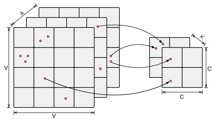
Figure 2: Compositional allocation. For clarity, we show the allocation process for a three-dimensional count tensor (ignoring time steps). Observed three-dimensional event tokens (left) are compositionally allocated to three-dimensional latent classes (right).

BPTD and other Poisson-based models yield allocation inference algorithms that take advantage of the inherent sparsity of the data and scale with the number of event tokens. In contrast, non-Poisson tensor decomposition models (including Hoff’s model) lead to algorithms that scale with the size of the count tensor. Allocation-based inference in BPTD is especially efficient because it compositionally allocates each $M$-dimensional event token to an $M$-dimensional latent class. Figure 2 illustrates this process. CP decomposition models, such as those of DuBois & Smyth (2010) and Schein et al. (2015), only permit non-compositional allocation. For example, while BPTD allocates each token $e_{n}\!=\!(i{\xrightarrow{a}}j,t)$ to a four-dimensional latent class $(c{\xrightarrow{k}}d,r)$, Schein et al.’s model allocates $e_{n}$ to a one-dimensional latent class $q$ that cannot be decomposed. Therefore, when $Q\!=\!C\times C\times K\times R$, BPTD yields a faster allocation inference algorithm than Schein et al.’s model.

5 Country–Country Interaction Event Data

Our data come from the Integrated Crisis Early Warning System (ICEWS) of Boschee et al. and the Global Database of Events, Language, and Tone (GDELT) of Leetaru & Schrodt (2013). ICEWS and GDELT both use the Conflict and Mediation Event Observations (CAMEO) hierarchy (Gerner et al., ) for senders, receivers, and actions.

The top-level CAMEO coding for senders and receivers is their country affiliation, while lower levels in the hierarchy incorporate more specific attributes like their sectors (e.g., government or civilian) and their religious or ethnic affiliations. When studying international relations using CAMEO-coded event data, researchers usually consider only the senders’ and receivers’ countries. There are 249 countries represented in ICEWS, which include non-universally recognized states, such as Occupied Palestinian Territory, and former states, such as Former Yugoslav Republic of Macedonia; there are 233 countries in GDELT.

The top level for actions, which we use in our analyses, consists of twenty action classes, roughly ranked according to their overall sentiment. For example, the most negative is 20—Use Unconventional Mass Violence. CAMEO further divides these actions into the QuadClass scheme: Verbal Cooperation (actions 2–5), Material Cooperation (actions 6–7), Verbal Conflict (actions 8–16), and Material Conflict (16–20). The first action (1—Make Statement) is neutral.

6 Predictive Analysis

Baseline models: We compared BPTD’s predictive performance to that of three baseline models, described in section 3: 1) GPIRM, 2) DCGPIRM, and 3) the Bayesian Poisson tensor factorization (BPTF) model of Schein et al. (2015). All three models use a Poisson likelihood and have the same two hyperparameters as BPTD—i.e., $\epsilon_{0}$ and $\gamma_{0}$. We set $\epsilon_{0}$ to 0.1, as recommended by Gelman (2006), and we set $\gamma_{0}$ so that $\left(\gamma_{0}\,/\,C\right)^{2}\left(\gamma_{0}\,/\,K\right)\left(\gamma_{0}\,/\,R\right)=0.01$. This parameterization encourages the elements of the core tensor $\boldsymbol{\Lambda}$ to be sparse. We implemented an MCMC inference algorithm for each model. We provide the full generative process for all three models in the supplementary material.

GPIRM and DCGPIRM are both Tucker decomposition models and thus allocate events to four-dimensional latent classes. The cardinalities of these latent dimensions are the same as BPTD’s—i.e., $C$, $K$, and $R$. In contrast, BPTF is a CP decomposition model and thus allocates events to one-dimensional latent classes. We set the cardinality of this dimension so that the total number of latent factors in BPTF’s likelihood was equal to the total number of latent factors in BPTD’s likelihood—i.e., $Q\!=\!\lceil\frac{(V\times C)+(A\times K)+(T\times R)+(C^{2}\times K\times R)}{V+V+A+T+1}\rceil$. We chose not to let BPTF and BPTD use the same number of latent classes—i.e., to set $Q\!=\!C^{2}\times K\times R$. BPTF does not permit non-compositional allocation, so MCMC inference becomes very slow for even moderate values of $C$, $K$, and $R$. CP decomposition models also tend to overfit when $Q$ is large (Zhao et al., 2015). Throughout our predictive experiments, we let $C\!=\!20$, $K\!=\!6$, and $R\!=\!3$. These values were well-supported by the data, as we explain in section 7.

Experimental setup: We constructed twelve different observed tensors—six from ICEWS and six from GDELT. Five of the six tensors for each source (ICEWS or GDELT) correspond to one-year time spans with monthly time steps, starting with 2004 and ending with 2008; the sixth corresponds to a five-year time span with monthly time steps, spanning 1995–2000. We divided each tensor $\boldsymbol{Y}$ into a training tensor $\boldsymbol{Y}_{\textrm{train}}\!=\!\boldsymbol{Y}^{(1)},\ldots,\boldsymbol{Y}^{(T-3)}$ and a test tensor $\boldsymbol{Y}_{\textrm{test}}\!=\!\boldsymbol{Y}^{(T-2)},\ldots,\boldsymbol{Y}^{(T)}$. We further divided each test tensor into a held-out portion and an observed portion via a binary mask. We experimented with two different masks: one that treats the elements involving the most active fifteen countries as the held-out portion and the remaining elements as the observed portion, and one that does the opposite. The first mask enabled us to evaluate the models’ reconstructions of the densest (and arguably most interesting) portion of each test tensor, while the second mask enabled us to evaluate their reconstructions of its complement. Across the entire GDELT database, for example, the elements involving the most active fifteen countries—i.e., 6% of all 233 countries—account for 30% of the event tokens. Moreover, 40% of these elements are non-zero. These non-zero elements are highly dispersed, with a variance-to-mean ratio of 220. In contrast, only 0.7% of the elements involving the other countries are non-zero. These elements have a variance-to-mean ratio of 26.

For each combination of the four models, twelve tensors, and two masks, we ran 5,000 iterations of MCMC inference on the training tensor. We clamped the country–community factors, the action–topic factors, and the core tensor and then inferred the time-step–regime factors for the test tensor using its observed portion by running 1,000 iterations of MCMC inference. We saved every tenth sample after the first 500. We used each sample, along with the country–community factors, the action–topic factors, and the core tensor, to compute the Poisson rate for each element in the held-out portion of the test tensor. Finally, we averaged these rates across samples and used each element’s average rate to compute its probability. We combined the held-out elements’ probabilities by taking their geometric mean or, equivalently, by computing their inverse perplexity. We chose this combination strategy to ensure that the models were penalized heavily for making poor predictions on the non-zero elements and were not rewarded excessively for making good predictions on the zero elements. By clamping the country–community factors, the action–topic factors, and the core tensor after training, our experimental setup is analogous to that used to assess collaborative filtering models’ strong generalization ability (Marlin, 2004).

Figure 3: Predictive performance. Each plot shows the inverse perplexity (higher is better) for the four models: the GPIRM (blue), the DCGPIRM (green), BPTF (red), and BPTD (yellow). In the experiments depicted in the top row, we treated the elements involving the most active countries as the held-out portion; in the experiments depicted in the bottom row, we treated the remaining elements as the held-out portion. For ease of comparison, we scaled the inverse perplexities to lie between zero and one; we give the scales in the top-left corners of the plots. BPTD outperformed the baselines significantly when predicting the denser portion of each test tensor (top row).

Results: Figure 3 illustrates the results for each combination of the four models, twelve tensors, and two masks. The top row contains the results from the twelve experiments involving the first mask, where the elements involving the most active fifteen countries were treated as the held-out portion. BPTD outperformed the baselines significantly. BPTF—itself a state-of-the-art model—performed better than BPTD in only one experiment. In general, the Tucker decomposition allows BPTD to learn richer latent structure that generalizes better to held-out data. The bottom row contains the results from the experiments involving the second mask. The models’ performance was closer in these experiments, probably because of the large proportion of easy-to-predict zero elements. BPTD and BPTF performed indistinguishably in these experiments, and both models outperformed the GPIRM and the DCGPIRM. The single-membership nature of the GPIRM and the DCGPIRM prevents them from expressing high levels of heterogeneity in the countries’ rates of activity. When the held-out elements were highly dispersed, these models sometimes made extremely inaccurate predictions. In contrast, the mixed-membership nature of BPTD and BPTF allows them to better express heterogeneous rates of activity.

7 Exploratory Analysis

We used a tensor of ICEWS events spanning 1995–2000, with monthly time steps, to explore the latent structure discovered by BPTD. We initially let $C\!=\!50$, $K\!=\!8$, and $R\!=\!3$—i.e., $C\times C\times K\times R=60,000$ latent classes—and used the shrinkage priors to adaptively learn the most appropriate numbers of communities, topics, and regimes. We found $C\!=\!20$ communities and $K\!=\!6$ topics with weights that were significantly greater than zero. We provide a plot of the community weights in the supplementary material. Although all three regimes had non-zero weights, one had a much larger weight than the other two. For comparison, Schein et al. (2015) used fifty latent classes to model the same data, while Hoff (2015) used $C\!=\!4$, $K\!=\!4$, and $R\!=\!4$ to model a similar tensor from GDELT.

Topics of action types: We show the inferred action–topic factors as a heatmap in the left subplot of figure 4. We ordered the topics by their weights $\nu_{1},\ldots,\nu_{K}$, which are above the heatmap. The inferred topics correspond very closely to CAMEO’s QuadClass scheme. Moving from left to right, the topics place their mass on increasingly negative actions. Topics 1 and 2 place most of their mass on Verbal Cooperation actions; topic 3 places most of its mass on Material Cooperation actions and the neutral 1—Make Statement action; topic 4 places most of its mass on Verbal Conflict actions and the 1—Make Statement action; and topics 5 and 6 place their mass on Material Conflict actions.

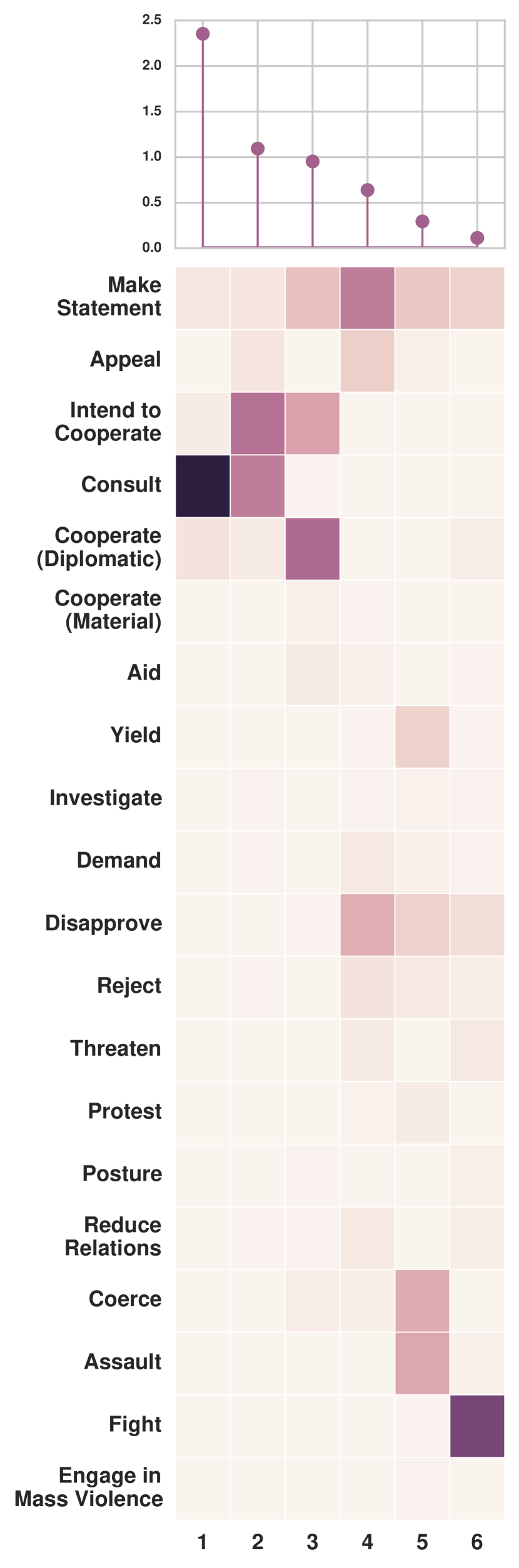
Figure 4: Left: Action–topic factors. The topics are ordered by $\nu_{1},\ldots,\nu_{K}$ (above the heatmap). Right: Latent structure discovered by BPTD for topic $k\!=\!1$ and the most active regime, including the community–community interaction network (bottom left), the rate at which each country acts as a sender (top left) and a receiver (bottom right) in each community, and the number of times each country $i$ took an action associated with topic $k$ toward each country $j$ during regime $r$ (top right). We show only the most active 100 countries.

Topic-partitioned community–community networks: In the right subplot of figure 4, we visualize the inferred community structure for topic $k\!=\!1$ and the most active regime $r$. The bottom-left heatmap is the community–community interaction network $\boldsymbol{\Lambda}^{(r)}_{k}$. The top-left heatmap depicts the rate at which each country $i$ acts as a sender in each community $c$—i.e., $\theta_{ic}\sum_{j=1}^{V}\sum_{d=1}^{C}\theta_{jd}\,\lambda^{(r)}_{c{\xrightarrow{k}}d}$. Similarly, the bottom-right heatmap depicts the rate at which each country acts as a receiver in each community. The top-right heatmap depicts the number of times each country $i$ took an action associated with topic $k$ toward each country $j$ during regime $r$—i.e., $\sum_{c=1}^{C}\sum_{d=1}^{C}\sum_{a=1}^{A}\sum_{t=1}^{T}y^{(tr)}_{ic{\xrightarrow{ak}}jd}$. We grouped the countries by their strongest community memberships and ordered the communities by their within-community interaction weights $\eta_{1}^{\,\mathbin{\text{\rotatebox[origin={c}]{90.0}{$\circlearrowright$}}}},\ldots,\eta_{C}^{\,\mathbin{\text{\rotatebox[origin={c}]{90.0}{$\circlearrowright$}}}}$, from smallest to largest; the thin green lines separate the countries that are strongly associated with one community from the countries that are strongly associated with its adjacent communities.

Some communities contain only one or two strongly associated countries. For example, community 1 contains only the US, community 6 contains only China, and community 7 contains only Russia and Belarus. These communities mostly engage in between-community interaction. Other larger communities, such as communities 9 and 15, mostly engage in within-community interaction. Most communities have a strong geographic interpretation. Moving upward from the bottom, there are communities that correspond to Eastern Europe, East Africa, South-Central Africa, Latin America, Australasia, Central Europe, Central Asia, etc. The community–community interaction network summarizes the patterns in the top-right heatmap. This topic is dominated by the 4–Consult action, so the network is symmetric; the more negative topics have asymmetric community–community interaction networks. We therefore hypothesize that cooperation is an inherently reciprocal type of interaction. We provide visualizations for the other five topics in the supplementary material.

8 Summary

We presented Bayesian Poisson Tucker decomposition (BPTD) for learning the latent structure of international relations from country–country interaction events of the form “country $i$ took action $a$ toward country $j$ at time $t$.” Unlike previous models, BPTD takes advantage of all three representations of an interaction event data set: 1) a set of event tokens, 2) a tensor of event type counts, and 3) a series of weighted multinetwork snapshots. BPTD uses a Poisson likelihood, respecting the discrete nature of the data and its inherent sparsity. Moreover, BPTD yields a compositional allocation inference algorithm that is more efficient than non-compositional allocation algorithms. Because BPTD is a Tucker decomposition model, it shares parameters across latent classes. In contrast, CP decomposition models force each latent class to capture potentially redundant information. BPTD therefore “does more with less.” This efficiency is reflected in our predictive analysis: BPTD outperforms BPTF—a CP decomposition model—as well as two other baselines. BPTD learns interpretable latent structure that aligns with well-known concepts from the networks literature. Specifically, BPTD learns latent country–community memberships, including the number of communities, as well as directed community–community interaction networks that are specific to topics of action types and temporal regimes. This structure captures the complexity of country–country interactions, while revealing patterns that agree with our knowledge of international relations. Finally, although we presented BPTD in the context of interaction events, BPTD is well suited to learning latent structure from other types of multidimensional count data.

References

- Airoldi et al. (2008) Airoldi, E. M., Blei, D. M., Feinberg, S. E., and Xing, E. P. Mixed membership stochastic blockmodels. Journal of Machine Learning Research, 9:1981–2014, 2008.
- Ball et al. (2011) Ball, B., Karrer, B., and Newman, M. E. J. Efficient and principled method for detecting communities in networks. Physical Review E, 84(3), 2011.
- Blei et al. (2003) Blei, D., Ng, A., and Jordan, M. Latent Dirichlet allocation. Journal of Machine Learning Research, 3:993–1022, 2003.
- (4) Boschee, E., Lautenschlager, J., O’Brien, S., Shellman, S., Starz, J., and Ward, M. ICEWS coded event data. Harvard Dataverse. V10.
- Cemgil (2009) Cemgil, A. T. Bayesian inference for nonnegative matrix factorisation models. Computational Intelligence and Neuroscience, 2009.
- Chi & Kolda (2012) Chi, E. C. and Kolda, T. G. On tensors, sparsity, and nonnegative factorizations. SIAM Journal on Matrix Analysis and Applications, 33(4):1272–1299, 2012.
- Cichocki et al. (2009) Cichocki, A., Zdunek, R., Phan, A. H., and i Amari, S. Nonnegative Matrix and Tensor Factorizations: Applications to Exploratory Multi-Way Data Analysis and Blind Source Separation. John Wiley & Sons, 2009.
- DuBois & Smyth (2010) DuBois, C. and Smyth, P. Modeling relational events via latent classes. In Proceedings of the Sixteenth ACM SIGKDD International Conference on Knowledge Discovery and Data Mining, pp. 803–812, 2010.
- Ferguson (1973) Ferguson, T. S. A Bayesian analysis of some nonparametric problems. The Annals of Statistics, 1(2):209–230, 1973.
- Gelman (2006) Gelman, A. Prior distributions for variance parameters in hierarchical models. Bayesian Analysis, 1(3):515–533, 2006.
- (11) Gerner, D. J., Schrodt, P. A., Abu-Jabr, R., and Yilmaz, Ö. Conflict and mediation event observations (CAMEO): A new event data framework for the analysis of foreign policy interactions. Working paper.
- Gopalan et al. (2014) Gopalan, P., Ruiz, F. J. R., Ranganath, R., and Blei, D. M. Bayesian nonparametric Poisson factorization for recommendation systems. In Proceedings of the Seventeenth International Conference on Artificial Intelligence and Statistics, volume 33, pp. 275–283, 2014.
- Gopalan et al. (2015) Gopalan, P., Hofman, J., and Blei, D. Scalable recommendation with Poisson factorization. In Proceedings of the Thirty-First Conference on Uncertainty in Artificial Intelligence, 2015.
- Harshman (1970) Harshman, R. Foundations of the PARAFAC procedure: Models and conditions for an “explanatory” multimodal factor analysis. UCLA Working Papers in Phonetics, 16:1–84, 1970.
- Hoff (2014) Hoff, P. Multilinear tensor regression for longitudinal relational data. arXiv:1412.0048, 2014.
- Hoff (2015) Hoff, P. Equivariant and scale-free Tucker decomposition models. Bayesian Analysis, 2015.
- Karrer & Newman (2011) Karrer, B. and Newman, M. E. J. Stochastic blockmodels and community structure in networks. Physical Review E, 83(1), 2011.
- Kemp et al. (2006) Kemp, C., Tenenbaum, J. B., Griffiths, T. L., Yamada, T., and Ueda, N. Learning systems of concepts with an infinite relational model. In Proceedings of the Twenty-First National Conference on Artificial Intelligence, 2006.
- Kim & Choi (20007) Kim, Y.-D. and Choi, S. Nonnegative Tucker decomposition. In Proceedings of the IEEE Conference on Computer Vision and Pattern Recognition, 20007.
- Kingman (1972) Kingman, J. F. C. Poisson Processes. Oxford University Press, 1972.
- Kolda & Bader (2009) Kolda, T. G. and Bader, B. W. Tensor decompositions and applications. SIAM Review, 51(3):455–500, 2009.
- Leetaru & Schrodt (2013) Leetaru, K. and Schrodt, P. GDELT: Global data on events, location, and tone, 1979–2012. Working paper, 2013.
- Marlin (2004) Marlin, B. Collaborative filtering: A machine learning perspective. Master’s thesis, University of Toronto, 2004.
- Mørup et al. (2008) Mørup, M., Hansen, L. K., and Arnfred, S. M. Algorithms for sparse nonnegative Tucker decompositions. Neural Computation, 20(8):2112–2131, 2008.
- Nickel et al. (2012) Nickel, M., Tresp, V., and Kriegel, H.-P. Factorizing YAGO: Scalable machine learning for linked data. In Proceedings of the Twenty-First International World Wide Web Conference, pp. 271–280, 2012.
- Nickel et al. (2015) Nickel, M., Murphy, K., Tresp, V., and Gabrilovich, E. A review of relational machine learning for knowledge graphs: From multi-relational link prediction to automated knowledge graph construction. arXiv:1503.00759, 2015.
- Nowicki & Snijders (2001) Nowicki, K. and Snijders, T. A. B. Estimation and prediction for stochastic blockstructures. Journal of the American Statistical Association, 96(455):1077–1087, 2001.
- Schein et al. (2015) Schein, A., Paisley, J., Blei, D. M., and Wallach, H. Bayesian Poisson tensor factorization for inferrring multilateral relations from sparse dyadic event counts. In Proceedings of the Twenty-First ACM SIGKDD International Conference on Knowledge Discovery and Data Mining, pp. 1045–1054, 2015.
- Schmidt & Mørup (2013) Schmidt, M. N. and Mørup, M. Nonparametric Bayesian modeling of complex networks: An introduction. IEEE Signal Processing Magazine, 30(3):110–128, 2013.
- Tucker (1964) Tucker, L. R. The extension of factor analysis to three-dimensional matrices. In Frederiksen, N. and Gulliksen, H. (eds.), Contributions to Mathematical Psychology. Holt, Rinehart and Winston, 1964.
- Welling & Weber (2001) Welling, M. and Weber, M. Positive tensor factorization. Pattern Recognition Letters, 22(12):1255–1261, 2001.
- Xu et al. (2012) Xu, Z., Yan, F., and Qi, Y. Infinite Tucker decomposition: Nonparametric Bayesian models for multiway data analysis. In Proceedings of the Twenty-Ninth International Conference on Machine Learning, pp. 1023–1030, 2012.
- Zhao et al. (2015) Zhao, Q., Zhang, L., and Cichocki, A. Bayesian CP factorization of incomplete tensors with automatic rank determination. IEEE Transactions on Pattern Analysis and Machine Intelligence, 37(9):1751–1763, 2015.
- Zhou (2015) Zhou, M. Infinite edge partition models for overlapping community detection and link prediction. In Proceedings of the Eighteenth International Conference on Artificial Intelligence and Statistics, pp. 1135–1143, 2015.
- Zhou & Carin (2012) Zhou, M. and Carin, L. Augment-and-conquer negative binomial processes. In Advances in Neural Information Processing Systems Twenty-Five, pp. 2546–2554, 2012.
- Zhou & Carin (2015) Zhou, M. and Carin, L. Negative binomial process count and mixture modeling. IEEE Transactions on Pattern Analysis and Machine Intelligence, 37(2):307–320, 2015.