Scene Grammars, Factor Graphs, and Belief Propagation

Abstract

We describe a general framework for probabilistic modeling of complex scenes and inference from ambiguous observations. The approach is motivated by applications in image analysis and is based on the use of priors defined by stochastic grammars. We define a class of grammars that capture relationships between the objects in a scene and provide important contextual cues for statistical inference. The distribution over scenes defined by a probabilistic scene grammar can be represented by a graphical model and this construction can be used for efficient inference with loopy belief propagation.

We show experimental results with two different applications. One application involves the reconstruction of binary contour maps. Another application involves detecting and localizing faces in images. In both applications the same framework leads to robust inference algorithms that can effectively combine local information to reason about a scene.

1 Introduction

We consider the problem of knowledge representation for scene understanding. The problem has a significant history in pattern recognition, artificial intelligence, and statistics (e.g., [26, 22, 39, 4, 47]). Our primary goal is to develop a general purpose framework for modeling complex scenes and for efficient inference and learning with such models.

The philosophy behind our approach follows Grenander’s Pattern Theory [26] program. A key idea in Pattern Theory is to model patterns in a variety of different settings using algebraic and probabilistic systems that define regular structures and probability distributions over these structures. The approach emphasizes the relationship between pattern analysis and pattern synthesis, and is based on the use of Bayesian statistics for inference of hidden structures.

In the Bayesian formulation of scene understanding a prior model captures the statistical regularities of scenes in the world. The prior model makes it possible to reason about typical scenes and to estimate a scene from partial or ambiguous observations. A significant challenge within this framework is to define a class of models that is both expressive and computationally tractable. That is, one would like to define models that can capture regular structures in a variety of applications and design efficient algorithms for inference with such models.

The general framework we describe in this paper is based on three key components: (1) A class of stochastic grammars for modeling complex scenes; (2) The construction of graphical models that represent scene distributions; and (3) An efficient method for approximate inference with loopy belief propagation.

The types of scenes we consider often lead to complex high-dimensional structures. For example, in Section 3.1 we consider scenes with faces and parts of faces. Even in this simple setting a scene can contain a variable number of objects and each object can be in many different locations. The number of possible scenes is very large (or infinite). Nonetheless scenes have regularities (e.g. faces have eyes). This is similar to the situation in formal language models where languages defined by grammars and automata often include an infinite set of well-formed sentences.

A probabilistic scene grammar defines a set of (regular) scenes and a probability distribution over scenes. Scenes are defined using a set of building blocks and a set of production rules. The productions define typical co-occurances of small groups of objects. Productions are chained together to form larger compositions, and this process leads to a large set of possible structures. The scenes generated by a scene grammar capture both the presence of different objects and relationships among them (such as part-of, or aligned-with). The set of scenes generated by a scene grammar defines a language of regular scenes. The set of scenes can also be seen as a state space and is similar to the configuration space in Pattern Theory.

A scene generated by a probabilistic scene grammar can be represented using a finite set of random variables. Importantly, we derive a product formula for the probability of a scene using this representation. This leads to a graphical model that can be used for inference via local message passing methods such as belief propagation ([39]).

Inference is a challenging computational problem. We describe an efficient method for inference using loopy belief propagation. The approach involves efficient computation of messages in the sum-product algorithm. This is possible due to the special structure of the graphical models that arise within our framework. Inference with loopy belief propagation aggregates information using the production rules in a grammar. For example, if a production rule generates the eyes, nose and mouth of a face, any evidence for the face or one of its parts provides contextual evidence for the whole composition.

Throughout the paper we describe examples of scene grammars that generate different kinds of scenes motivated by problems in computer vision and image analysis. We illustrate the results of numerical experiments with these models, both for reasoning about abstract scenes and in practical applications. All of the numerical experiments were performed using a common implementation of a general computational engine.

We include experimental results with two applications. One application involves detecting curves in noisy images and reconstructing binary contour maps. We address this problem using a grammar that generates scenes with a collection of regular curves. Another application involves detecting faces and parts of faces in images. In this case we use a grammar that captures spatial relationships between the parts that make up a face. In both applications the framework and computational methods described here lead to good experimental results.

1.1 Motivation and Related Work

Formal grammars, and in particular context-free grammars, have been widely used for modeling the structure of sentences in natural language ([9, 34]). Similar models have been used to represent patterns in biological structures such as DNA and RNA ([14]). Grammars are also commonly used to define the syntax of programming languages ([1]).

In computer graphics the recursive description of objects using grammars and rewriting systems has been used to generate complex geometric objects, biological structures, and landscapes ([40, 13]). These methods illustrate the potential that (stochastic) grammars have for modeling natural and man-made structures.

Since the early days of image analysis attempts have been made to develop formal language models for two-dimensional pictures (see, e.g., [41]). There are significant challenges in designing effective models and algorithms for parsing images using grammars, including the fact that the pixels in an image are not linearly ordered. One important difference between parsing images and parsing sentences is the number of possible constituents. The number of continuous subsentences of a sentence of length $n$ is quadratic in $n$. On the other hand, the number of connected regions in an image with $n$ pixels is exponential in $n$. This means that classical parsing algorithms based on dynamic programming over constituents cannot be easily applied to images.

The interpretation of scenes via repeated application of grouping rules is one of the key ideas behind the Gestalt theory of visual perception ([38]). The structures generated by a scene grammar are similar to the hierarchical description of a scene using grouping rules. The approach is also related to the description of scenes using compositional models and the MDL principle [5].

Statistical models and Bayesian inference methods have been previously used to solve a variety of problems in computer vision and image analysis (e.g., [4, 24, 8, 35, 23, 2, 18]). Probabilistic scene grammars provide a unified framework to address many of these problems.

Probabilistic scene grammars generalize part-based models for object detection and recognition such as pictorial structures [21, 18] and constellations of features [6]. In a grammar model objects can be defined using a hierarchy of reusable parts. Probabilistic scene grammars can also represent objects with variable structure (when the parts that make up an object can change) and scenes with multiple objects. Furthermore, the use of recursion allows for modeling complex objects, such as curves of varying lengths and shape, using a small finite set of production rules.

Besides allowing for the definition of very general models, grammars also provide a useful conceptual abstraction to reason about models and shared parameters.

Figure 1 shows an example of a set of production rules in a grammar that can generate scenes with multiple people that are composed of different parts. In this case a person always has parts corresponding to the face, arms, and lower-body. Some faces have hats while other faces do not, and hats can be of different types. Similarly some people wear skirts while other people wear pants. Since we have multiple independent choices for the rules used to expand different symbols we see a combinatorial explosion in the number of possible structures that can be generated with a small number of rules.

$$\mathrm{PERSON} \rightarrow\mathrm{FACE},\mathrm{ARMS},\mathrm{LOWER}$$

$$\mathrm{FACE} \rightarrow\mathrm{EYES},\mathrm{NOSE},\mathrm{MOUTH}$$

$$\mathrm{FACE} \rightarrow\mathrm{HAT},\mathrm{EYES},\mathrm{NOSE},\mathrm{MOUTH}$$

$$\mathrm{EYES} \rightarrow\mathrm{EYE},\mathrm{EYE}$$

$$\mathrm{EYES} \rightarrow\mathrm{SUNGLASSES}$$

$$\mathrm{HAT} \rightarrow\mathrm{BASEBALL}$$

$$\mathrm{HAT} \rightarrow\mathrm{SOMBRERO}$$

$$\mathrm{LOWER} \rightarrow\mathrm{SHOE},\mathrm{SHOE},\mathrm{LEGS}$$

$$\mathrm{LEGS} \rightarrow\mathrm{PANTS}$$

$$\mathrm{LEGS} \rightarrow\mathrm{SKIRT}$$

Figure 1: Production rules in a grammar that generates scenes with people. The parts that make up a person can vary and a small set of rules can generate a large number of structures.

Probabilistic scene grammars are closely related to the Markov backbone in [30]. Other related work includes [25, 46, 53, 52, 51, 19]. These methods have generally relied on MCMC or heuristic methods for inference, or dynamic programming for restricted models. The approach we develop here using loopy belief propagation is related to the dynamic programming approach but can be applied in a more general setting.

Several probabilistic programming languages have been designed with the goal of providing a general framework for probabilistic modeling and inference. For example, the Picture and Edward frameworks ([33, 45]) share the high-level goal of having a general-purpose modeling system for scene understanding. These methods seek high-probability scenes encoded as probabilistic program traces via MCMC and variational inference. The scene grammars we define are closely related to a probabilistic program where all functions are “memoized” (in the sense of dynamic programming). This allows for the representation of all possible program traces with a finite graphical model and for the implicit reasoning about program execution via loopy belief propagation.

1.2 Overview

In Section 2 we define a class of probabilistic scene grammars and the generative process used to generate scenes. In Section 3 we give examples of scene grammars that generate different types of scenes. In Section 4 we derive a product formula for the probability of a scene and define a general method for constructing graphical models that represent scene distributions. In Section 5 we describe an efficient inference method based on loopy belief propagation and in Section 6 we illustrate the result of inference using the example grammars from Section 3. Section 7 considers the problem of learning model parameter using maximum-likelihood estimation. In Section 8 we illustrate the results of our methods in two different applications.

2 Probabilistic Scene Grammars

Our goal is to reason about scenes and to estimate a description of a scene from a set of observations. A key component of the approach is a prior model over scenes, $p(S)$, that captures the statistical regularities of scenes in the world.

A probabilistic scene grammar defines a set of possible scenes and a probability distribution over scenes. Scenes are defined using a set of building blocks, or bricks, that are connected together using a set of basic compositions, or production rules.

To generate scenes we define a random process that grows a scene starting from an initial set of bricks. Initially every brick is considered to be included in the scene independently. We then repeatedly use production rules to expand (or grow) bricks that are in the scene but have not been expanded before. The result of this process defines a distribution, $p(S)$, that can capture regularities in natural scenes. For example, the process can capture which objects tend to co-occur in a scene and the typical relative positions between such objects.

Each brick is defined by a pair consisting of a symbol and a pose. For example, one brick might be the pair $(\operatorname*{\mathsf{FACE}},(30,40))$ representing a face at location $(30,40)$ in an image.

In a probabilistic scene grammar the initial generation of bricks is governed by self-rooting probabilities. The possible expansions of a brick are determined by a set of production rules, rule selection probabilities and conditional pose distributions.

Let $\Sigma$ be a finite set. We use $\Sigma^{*}$ to denote the set of finite strings of elements from $\Sigma$, including the empty string.

Definition 2.1.

A probabilistic scene grammar (PSG) is defined by a 6-tuple $\mathcal{G}=(\Sigma,\Omega,\mathcal{R},q,\rho,\epsilon)$, where

1. $\Sigma$ is a finite set (the symbols).

2. $\Omega=\{\,\Omega_{A}\mid A\in\Sigma\,\}$ where $\Omega_{A}$ is a finite set (the pose spaces).

3. $\mathcal{R}$ is a finite subset of $\Sigma\times\Sigma^{*}$ (the production rules).

   A production rule is specified in the form $A_{0}\rightarrow A_{1},\ldots,A_{n}$ where $n\geq 0$ and $A_{i}\in\Sigma$.

   For $r\in\mathcal{R}$ we use $n_{r}$ to denote the number of symbols in the right-hand-side of $r$ and $A_{(r,i)}$ to denote the $i$-th symbol in $r$.

   Let $\mathcal{R}_{A}$ be the set of rules with $A\in\Sigma$ in the left-hand-side. We assume $R_{A}\neq\emptyset$.

4. $q=\{\,q_{A}\mid A\in\Sigma\,\}$ where $q_{A}$ is a distribution over $\mathcal{R}_{A}$ (the rule selection probabilities).

5. $\rho=\{\,\rho_{(r,i)}\mid r\in\mathcal{R},\,1\leq i\leq n_{r}\,\}$ is a set of conditional pose distributions.

   For a rule $r=A_{0}\rightarrow A_{1},\ldots,A_{n}$ we have $\rho_{(r,i)}:\Omega_{A_{i}}\times\Omega_{A_{0}}\rightarrow\mathbb{R}_{\geq 0}$ with

   $$\sum_{\omega_{i}\in\Omega_{A_{i}}}\rho_{(r,i)}(\omega_{i},\omega_{0})=1,\;\;\ \forall\omega_{0}\in\Omega_{A_{0}}.$$

   We use $\rho_{(r,i)}(\omega_{i}|\omega_{0})$ to denote $\rho_{(r,i)}(\omega_{i},\omega_{0})$.

6. $\epsilon=\{\,\epsilon_{A}\mid A\in\Sigma\,\}$ where $0\leq\epsilon_{A}\leq 1$ (the self-rooting probabilities).

The definition of a probabilistic scene grammar is closely related to the definition of a probabilistic context-free grammar (PCFG) used in formal language models and in natural language processing (see, e.g., [34]). However, the structures that are generated by a scene grammar are different from the structures generated by a PCFG (see Remark 2.5).

Let $\mathcal{G}=(\Sigma,\Omega,\mathcal{R},q,\rho,\epsilon)$ be a scene grammar. The structure of a scene is defined by $(\Sigma,\Omega,\mathcal{R})$ and the parameters $(q,\rho,\epsilon)$ define a (non-uniform) probability distribution over “well-formed” scenes. In practice we assume $\rho_{(r,i)}(\omega_{i}|\omega)$ is invariant to a set of transformations (such as translations) of the pose spaces and this significantly reduces the number of parameters in the model.

Definition 2.2.

The bricks defined by a scene grammar $\mathcal{G}$ are pairs of symbols and poses,

$$\mathcal{B}=\{\,(A,\omega)\mid A\in\Sigma,\omega\in\Omega_{A}\,\}.$$

Definition 2.3.

A scene $S$ generated by $\mathcal{G}$ is defined by:

1. A subset $O\subseteq\mathcal{B}$ of bricks that are present in $S$.

2. For each $(A,\omega)\in O$ a selection of rule $A\rightarrow A_{1},\ldots,A_{n}\in\mathcal{R}$ and poses $\omega_{i}$ such that $(A_{i},\omega_{i})\in O$ for $1\leq i\leq n$. We say $(A,\omega)$ expands to, or is a parent of, $(A_{i},\omega_{i})$ in $S$.

Let $\mathcal{S}$ be the set of scenes generated by a grammar $\mathcal{G}$. The set $\mathcal{S}$ is the “Language” generated by $\mathcal{G}$. Note that each $S\in\mathcal{S}$ specifies both a set of objects that are present in the scene (the bricks) and relationships between these objects.

To define the scene generation process we use a set $O$ to keep track of bricks in the scene and a set $Q$ to keep track of a queue of bricks that are in the scene but have not been expanded yet. Initially bricks are included in the scene independently, according to self-rooting probabilities. All of these bricks are queued for expansion. The process terminates when all bricks in the scene have been expanded ($Q$ is empty). If an expansion generates a brick that is not already in the scene we add the brick to the scene and queue it for expansion.

Definition 2.4.

Random scene generation with a grammar $\mathcal{G}=(\Sigma,\Omega,\mathcal{R},q,\rho,\epsilon)$.

1. Initially $O=\emptyset$ and $Q=\emptyset$.

2. For each brick $(A,\omega)\in\mathcal{B}$ add $(A,\omega)$ to both $O$ and $Q$ with probability $\epsilon_{A}$.

3. While $Q\neq\emptyset$ remove a brick $(A,\omega)$ from $Q$ and expand it.

4. Expanding $(A,\omega)$ involves

   1. Sampling a rule $r=A\rightarrow A_{1},\ldots,A_{n}\in\mathcal{R}$ according to $q_{A}$.

   2. Sampling poses $\omega_{i}$ according to $\rho_{(r,i)}(\omega_{i}|\omega)$.

   3. If $(A_{i},\omega_{i})\not\in O$ add it to both $O$ and $Q$.

The output of the process is a scene $S$ defined by $O$ and the rules and poses selected when expanding each brick in $O$.

The scene generation process always terminates after at most $|\mathcal{B}|$ expansions. When the process terminates every brick in $O$ will have been expanded exactly once, and therefore the output is a valid scene $S\in\mathcal{S}$. We note that the order in which the bricks in $Q$ are selected for expansion does not influence the probability, $p(S)$, of generating a scene.

The self-rooting probabilities, $\epsilon_{A}$, control the number of bricks that are included in the scene initially, before any bricks are expanded. For $A\in\Sigma$ the expected number of bricks of type $A$ that self-root is $\epsilon_{A}|\Omega_{A}|$. Since the pose spaces are often very large, the self-rooting probabilities are usually very small. Note however that even if a brick $(A,\omega)$ self-roots, another brick $(B,z)$ may expand and become a parent of $(A,\omega)$. The number of self-rooted bricks is an upper bound on the number of bricks with no parents.

Remark 2.5.

Scene grammars are related to PCFGs used in language modeling but they generate different types of structures.

Recall that a PCFG generates rooted derivation trees, where the vertices are labeled with symbols from a finite alphabet. In a derivation tree there is a single vertex (the root) with no parents and every other vertex has a unique parent.

A scene generated by a PSG defines a scene graph $G$ over the bricks that are present in the scene. The edges of $G$ capture which bricks expand to each other. The scene graph $G$ resembles a derivation tree generated by a PCFG, but it has more general connectivity structure. In particular there can be multiple vertices with no parents (roots) in $G$, and the graph can have multiple disjoint components. There can also be vertices with multiple parents in $G$. The scene graph $G$ can also have directed cycles, when a brick leads to a sequence of expansions that eventually generates the same brick again.

Finally we note that every scene graph is a subgraph of the complete directed graph over $\mathcal{B}$, and the number of possible scene graphs is finite (although it can be very large). This is in contrast to the fact that a context-free grammar can generate trees of unbounded size.

3 Example Grammars

In this section we give examples of PSGs and illustrate the random scenes they generate.

As described in Section 2 a scene grammar $\mathcal{G}$ is defined by a 6-tuple $(\Sigma,\Omega,\mathcal{R},q,\rho,\epsilon)$. In the examples below we combine the description of $\mathcal{R}$, $q$ and $\rho$ to simplify the notation. Let $r=A_{0}\rightarrow A_{1},\ldots,A_{n}$ be a rule in $\mathcal{R}$. To specify the rule, $r$, the rule selection probability, $q_{r}$, and the conditional pose distributions, $\rho_{(r,i)}$, we write,

$$\begin{array}[]{llll}q_{r},&(A_{0},\omega_{0})&\rightarrow&(A_{1},\rho_{(r,i)}(\cdot|\omega_{0})),\ldots,(A_{n},\rho_{(r,n)}(\cdot|\omega_{0})).\end{array}$$

In the examples in this section the pose spaces are grids of integer points $[N_{1}]\times\cdots\times[N_{D}]$, where $[N]=\{0,\ldots,N-1\}$. Let $a$ and $b$ be two points in a grid. We use $\operatorname*{UniformRect}(a,b)$ to denote a uniform distribution over grid points in the rectangular region with corners $a$ and $b$. We use $\delta(a)$ to denote the distribution concentrated at $a$.

3.1 Scenes with Faces

Grammar 1 generates scenes with faces and parts of faces. Figure 2 illustrates four random scenes generated by this grammar. The model captures the notion that faces have certain parts at appropriate locations. This is similar to other part-based representations such as pictorial structures (e.g. [21] and [18]) and deformable part models ([17]). However, the grammar generates scenes with multiple faces. It also allows for parts of faces to appear on their own, capturing the notion that a scene is made up of faces and other components that look like parts of faces.

 

$\Sigma=\{\operatorname*{\mathsf{FACE}},\operatorname*{\mathsf{EYE}},\operatorname*{\mathsf{NOSE}},\operatorname*{\mathsf{MOUTH}}\}$.

$\forall A\in\Sigma,\;\Omega_{A}=[N]\times[M]$.

Rules:

$\begin{array}[]{lllll}(1)&1.0,&(\operatorname*{\mathsf{FACE}},(x,y))&\rightarrow&(\operatorname*{\mathsf{EYE}},\operatorname*{UniformRect}((x,y)+a_{1},(x,y)+b_{1})),\\ &&&&(\operatorname*{\mathsf{EYE}},\operatorname*{UniformRect}((x,y)+a_{2},(x,y)+b_{2})),\\ &&&&(\operatorname*{\mathsf{NOSE}},\operatorname*{UniformRect}((x,y)+a_{3},(x,y)+b_{3})),\\ &&&&(\operatorname*{\mathsf{MOUTH}},\operatorname*{UniformRect}((x,y)+a_{4},(x,y)+b_{4})).\\ (2)&1.0,&(\operatorname*{\mathsf{EYE}},(x,y))&\rightarrow&\emptyset.\\ (3)&1.0,&(\operatorname*{\mathsf{NOSE}},(x,y))&\rightarrow&\emptyset.\\ (4)&1.0,&(\operatorname*{\mathsf{MOUTH}},(x,y))&\rightarrow&\emptyset.\end{array}$

$\epsilon_{\operatorname*{\mathsf{FACE}}}=10^{-4}.$

$\epsilon_{\operatorname*{\mathsf{EYE}}}=\epsilon_{\operatorname*{\mathsf{NOSE}}}=\epsilon_{\operatorname*{\mathsf{MOUTH}}}=10^{-5}.$

 

Grammar 1: A grammar for scenes with faces and parts of faces.

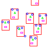
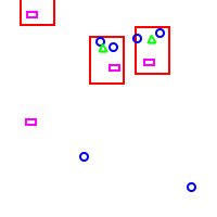
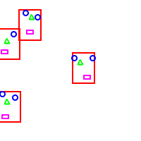
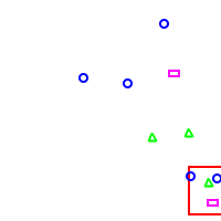
Figure 2: Random scenes generated using Grammar 1. Faces are represented by red rectangles, eyes by blue circles, noses by green triangles, and mouths by magenta rectangles. Scenes have multiple objects and parts of faces can appear both in the context of a face and on their own. The location of each face part can vary within a range of possible locations relative to the face.

In this grammar the pose of a brick specifies a 2D discrete location for an object (face, eye, nose or mouth) of fixed size and orientation. Rule (1) defines a part-based model for faces. The location of each face part is selected at random from a rectangular region defined relative to the location of the face. Figure 3 illustrates the possible locations for the parts that make up a face at one location. The self-rooting probabilities of the part symbols are smaller than the self-rooting probability of the face symbol, so that most parts appear in the context of a face.

In Section 6.1 we show how this model can be used for reasoning about scenes with faces. In Section 8.2 we show how a similar model can be used for face detection.

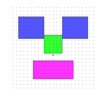
Figure 3: Possible locations for each face part when expanding a face at the red-cross location. The location of each part is selected uniformly at random from a rectangular region. The regions for the eyes, nose, and mouth are shown in blue, green and magenta.

The grammar defined here can be extended to represent objects of different sizes (and orientations) if we augment the pose spaces with scale (and orientation) information. The parts of the face can also be defined in terms of smaller parts (such as eyebrow and pupil for an eye). The grammar can also be extended to define scenes with many types of objects, and where objects of different types are defined using a set of reusable parts. By including additional productions rules in the grammar we can also define objects with variable structure.

3.2 Scenes with Curves

Grammar 2 generates scenes with discrete curves in a finite two-dimensional grid. The grammar generates scenes with a random number of curves and where each curve has a random length and shape, giving preference to curves with low curvature everywhere. As discussed in [42] these are the types of curves that are often perceptually salient to humans.

The process that generates an individual curve with Grammar 2 traces the path of a particle undergoing stochastic motion. Similar models were introduced in [36] and [49] in the context of contour completion. Figure 4 shows four random images generated by the grammar. In Section 6.2 we show how this model can be used for contour completion. In Section 8.1 we show how the model can be used to detect curves in noisy images and to reconstruct binary contour maps.

 

$\Sigma=\{\operatorname*{\mathsf{C}},\operatorname*{\mathsf{P}}\}$.

$\Omega_{\operatorname*{\mathsf{C}}}=[N]\times[M]\times[8]$.

$\Omega_{\operatorname*{\mathsf{P}}}=[N]\times[M]$.

Rules:

$\begin{array}[]{lllll}(1)&0.65,&(\operatorname*{\mathsf{C}},(x,y,\theta))&\rightarrow&(\operatorname*{\mathsf{P}},\delta((x,y))),(\operatorname*{\mathsf{C}},\delta(((x,y)+\operatorname*{round}(T_{\theta}(1,0)),\theta))).\\ (2)&0.124,&(\operatorname*{\mathsf{C}},(x,y,\theta))&\rightarrow&(\operatorname*{\mathsf{P}},\delta((x,y))),(\operatorname*{\mathsf{C}},\delta(((x,y)+\operatorname*{round}(T_{\theta-1}(1,0)),\theta))).\\ (3)&0.124,&(\operatorname*{\mathsf{C}},(x,y,\theta))&\rightarrow&(\operatorname*{\mathsf{P}},\delta((x,y))),(\operatorname*{\mathsf{C}},\delta(((x,y)+\operatorname*{round}(T_{\theta+1}(1,0)),\theta))).\\ (4)&0.05,&(\operatorname*{\mathsf{C}},(x,y,\theta))&\rightarrow&(\operatorname*{\mathsf{C}},\delta((x,y,\theta-1))).\\ (5)&0.05,&(\operatorname*{\mathsf{C}},(x,y,\theta))&\rightarrow&(\operatorname*{\mathsf{C}},\delta((x,y,\theta+1))).\\ (6)&0.002,&(\operatorname*{\mathsf{C}},(x,y,\theta))&\rightarrow&(\operatorname*{\mathsf{P}},\delta((x,y))).\\ (7)&1.00,&(\operatorname*{\mathsf{P}},(x,y))&\rightarrow&\emptyset.\end{array}$

$\epsilon_{\operatorname*{\mathsf{C}}}=\epsilon_{\operatorname*{\mathsf{P}}}=10^{-5}$.

 

The function $T_{\theta}$ denotes a rotation in the plane by a discrete angle $\theta$ and $\operatorname*{round}$ maps a point in the plane to the nearest grid point.

Grammar 2: A grammar for scenes with discrete curves.

Figure 4: Random images generated using Grammar 2. The grammar generates scenes with multiple curves of varying lengths and shapes, giving a preference to curves with low curvature. In each image the black pixels represent the $\operatorname*{\mathsf{P}}$ bricks that are part of a scene.

The grammar has two symbols, $\Sigma=\{\operatorname*{\mathsf{C}},\operatorname*{\mathsf{P}}\}$. The $\operatorname*{\mathsf{C}}$ bricks represent oriented elements (or particle states) that are generated in a sequence using a recursive rule to form discrete curves. The pose of a $\operatorname*{\mathsf{C}}$ brick specifies a location in an $[N]\times[M]$ pixel grid and one of 8 possible discrete orientations. The $\operatorname*{\mathsf{P}}$ bricks represent the trace of the curves in the pixel grid. The pose of a $\operatorname*{\mathsf{P}}$ brick specifies only a grid location and has no orientation information.

Rules (1)-(3) capture the possible extensions of a curve along a direction close to the current orientation. Figure 5 illustrates the possible extensions defined by rules (1)-(3) for a horizontal brick. When we extend a curve at pixel $(x,y)$ with orientation $\theta$, we move to one of 3 neighbors of $(x,y)$ that are approximately in the direction $\theta$. The curves generated are therefore contiguous. As we generate a curve we also generate $\operatorname*{\mathsf{P}}$ bricks tracing the path of the curve.

Figure 5: Possible extensions of a curve by one pixel. A horizontal $\operatorname*{\mathsf{C}}$ brick (in red) expands to one of three possible horizontal $\operatorname*{\mathsf{C}}$ bricks (in blue) with certain probabilities. The remaining probability mass is reserved for the choice to end the curve or change its orientation.

Rules (4)-(5) capture changes in orientation and rule (6) captures the termination of a curve. The probability of changing orientation is small, therefore curves tend to take multiple steps with a single discrete orientation before turning. This leads to curves with “low curvature” almost everywhere. The probability of selecting rule (6) controls the expected length of a curve.

4 Graphical Model

A PSG defines a probability distribution over a set of scenes. In this section we consider a representation of scenes using a finite set of random variables, and derive a closed form expression for the probability of a scene using a product of local functions. This leads to an undirected graphical model that can be used for inference (Section 5) and for learning model parameters (Section 7).

We start by defining a representation of scenes using binary random variables.

Let $\rho=\{\,\rho_{(r,i)}\,\}$ be the conditional pose distributions associated with a scene grammar $\mathcal{G}$. Let $\Gamma_{(r,i,\omega)}$ denote the support of $\rho_{(r,i)}(\cdot\,|\,\omega)$,

$$\Gamma_{(r,i,\omega)}=\{\,z\in\Omega_{A_{(r,i)}}\mid\rho_{(r,i)}(z\,|\,\omega)>0\,\}.$$

Definition 4.1.

Let $\mathcal{G}$ be a scene grammar and $S$ be a random scene generated by the grammar. Define the following random variables associated with each brick $(A,\omega)\in\mathcal{B}$,

$$X(A,\omega)\in\{0,1\},$$

$$R(A,\omega)=\{\,R(A,\omega,r)\in\{0,1\}\mid r\in\mathcal{R}_{A}\,\},$$

$$C(A,\omega)=\{\,C(A,\omega,r,i,z)\in\{0,1\}\mid r\in\mathcal{R}_{A},1\leq i\leq n_{r},z\in\Gamma_{(r,i,\omega)}\,\},$$

where

$X(A,\omega)=1$ iff $(A,\omega)$ is in $S$,

$R(A,\omega,r)=1$ iff rule $r$ is used to expand $(A,\omega)$ in $S$,

$C(A,\omega,r,i,z)=1$ iff $(A,\omega)$ is expanded with rule $r$ in $S$, and $z$ is the pose selected for $A_{(r,i)}$.

Remark 4.2.

A scene $S$ is uniquely defined by the value of the random variables $\{X,R,C\}$.

4.1 Product Formula

We now consider a class of acyclic PSGs and derive an expression for the probability of a scene, $p(S)$, using a product of local functions. This expression is analogous to the expression of the joint distribution in a Bayesian network. For the case of cyclic grammars the product expression can be used as a tractable approximation to $p(S)$.

Let $\mathcal{G}$ be a PSG with a set of bricks $\mathcal{B}$. We say $\mathcal{G}$ is acyclic if there is no sequence of expansions that generates a brick starting from itself. Equivalently, let $H$ be the directed graph over $\mathcal{B}$, with an edge from $(A,\omega)$ to $(B,z)$ if $(A,\omega)$ can generate $(B,z)$ in one expansion. The grammar $\mathcal{G}$ is acyclic if $H$ is an acyclic directed graph. For example, the grammar for scenes with faces in Section 3.1 is acyclic. On other other hand, the grammar for scenes with curves in Section 3.2 is cyclic.

A topological ordering of $\mathcal{B}$ is a linear ordering of $\mathcal{B}$ such that $(A,\omega)$ appears before $(B,z)$ whenever $(A,\omega)$ can generate $(B,z)$ after one or more expansions. When $\mathcal{G}$ is acyclic there is always a topological ordering of $\mathcal{B}$ and such an ordering can be computed by topologically sorting the vertices of $H$ (see, e.g., [10]).

There are two types of potential functions in the factorization of $p(X,R,C)$.

Definition 4.3.

A leaky-OR potential $\Psi^{L}_{\epsilon}(y,z)$ is a function of a $d$-dimensional binary vector $y$ (the input) and a binary value $z$ (the output). It encodes the conditional probability of each output value in a probabilistic OR gate. For a binary vector $y$ let $c(y)$ be the number of ones in $y$. If $c(y)>0$ we have $z=1$ with probability $1$. If $c(y)=0$ we have $z=1$ with probability $\epsilon$.

$$\Psi^{L}_{\epsilon}(y,z)=\begin{cases}1&c(y)>0,\,z=1,\\ 0&c(y)>0,\,z=0,\\ \epsilon&c(y)=0,\,z=1,\\ 1-\epsilon&c(y)=0,\,z=0.\end{cases}$$

Definition 4.4.

A selection potential $\Psi^{S}_{\theta}(y,z)$ is a function of a binary value $y$ (the input) and a $d$-dimensional binary vector $z$ (the output). It encodes the conditional probability of each output vector in a switch with $d$ binary outputs. If $y=0$ no output is selected with probability $1$. If $y=1$ a single output is selected according to probabilities defined by $\theta\in\mathbb{R}^{d}$.

$$\Psi^{S}_{\theta}(y,z)=\begin{cases}1&y=0,\,c(z)=0,\\ 0&y=0,\,c(z)>0,\\ 0&y=1,\,c(z)\neq 1,\\ \theta_{i}&y=1,\,c(z)=1,\,z_{i}=1.\end{cases}$$

To formulate the expression for $p(X,R,C)$ we also need to define the following collections of random variables,

$$C(A,\omega,r,i) = \{\,C(A,\omega,r,i,z)\mid z\in\Gamma_{(r,i,\omega)}\,\},$$

$$\operatorname*{parents}(X(A,\omega)) = \{\,C(B,z,r,i,\omega)\mid(B,z)\in\mathcal{B},r\in\mathcal{R}_{B},1\leq i\leq n_{r},A_{(r,i)}=A,\omega\in\Gamma_{(r,i,z)}\,\}.$$

Let $(A,\omega)$ be a brick. The set $C(A,\omega,r,i)$ includes all the random variables that specify the $i$-th child of $(A,\omega)$ if rule $r$ is used to expand $(A,\omega)$. The set $\operatorname*{parents}(X(A,\omega))$ includes all the random variables that specify the parents of $(A,\omega)$.

Theorem 4.5.

The distribution $p(X,R,C)$ defined by an acyclic grammar $\mathcal{G}$ can be expressed as,

$$p(X,R,C)=\\ \prod_{(A,\omega)\in\mathcal{B}}\left(p(X(A,\omega)\,|\,\operatorname*{parents}(X(A,\omega)))\,p(R(A,\omega)\,|\,X(A,\omega))\prod_{\begin{subarray}{c}r\in\mathcal{R}_{A},\\ 1\leq i\leq n_{r}\end{subarray}}p(C(A,\omega,r,i)\,|\,R(A,\omega,r))\right).$$ (1)

Moreover if $\mathcal{G}$ is acyclic,

1. $p(X(A,\omega)=z\,|\,\operatorname*{parents}(X(A,\omega))=y)=\Psi^{L}_{\epsilon_{A}}(y,z),$

2. $p(R(A,\omega)=z\,|\,X(A,\omega)=y)=\Psi^{S}_{q_{A}}(y,z),$

3. $p(C(A,\omega,r,i)=z\,|\,R(A,\omega,r)=y)=\Psi^{S}_{\rho_{(r,i)}}(y,z).$

Proof.

Let $V_{j}=\{X_{j},R_{j},C_{j}\}$ denote the random variables associated with the $j$-th brick in a topological ordering of $\mathcal{B}$. We can write

$$p(X,R,C) =\prod_{j}p(V_{j}\,|\,V_{k<j})$$

$$=\prod_{j}p(X_{j}\,|\,V_{k<j})p(R_{j}\,|\,X_{j},V_{k<j})p(C_{j}\,|\,R_{j},X_{j},V_{k<j}).$$

Based on the definition of the scene generation algorithm, and using the topological ordering constraint we see that

$$p(X_{j}\,|\,V_{k<j}) =p(X_{j}\,|\,\operatorname*{parents}(X_{j})),$$

$$p(R_{j}\,|\,X_{j},V_{k<j}) =p(R_{j}\,|\,X_{j}),$$

$$p(C_{j}\,|\,R_{j},X_{j},V_{k<j}) =p(C_{j}\,|\,R_{j}).$$

This leads to the expression for $p(X,R,C)$ above. The expression of each term in the factorization using the leaky-OR and selection potentials also follows directly from the definition of the scene generation algorithm and the topological ordering constraint. ∎

4.2 Factor Graph Construction

We now give a general construction for defining a graphical model that represents a probability distribution over scenes.

A factor graph (see, e.g., [32]) is an undirected graphical model that defines a probability distribution using a product of local functions. Let $\mathcal{F}=(V\cup F,E)$ be a bipartite graph where $V$ is a set of (discrete) random variables, $F$ is a set of factors and $E$ is a set of edges connecting variables to factors. Let $\mathcal{N}(u)$ denote the neighbors of a node $u$. Let $x$ denote an outcome for the variables in $V$. For $U\subseteq V$ we use $x_{U}$ to denote the values of the variables in $U$. Let $\Psi_{f}$ be a non-negative potential function associated with a factor $f\in F$. The factor graph $\mathcal{F}$ defines a joint distribution,

$$q(x)=\frac{1}{Z}\prod_{f\in F}\Psi_{f}(x_{\mathcal{N}(f)}),$$

where the normalizing constant $Z$ is selected so that $q$ sums to one.

Definition 4.6.

Let $\mathcal{G}$ be a scene grammar. Define the factor graph $\mathcal{F}(\mathcal{G})=(V\cup F,E)$ as follows:

1. The variables in $V$ correspond to the variables associated with a scene in Definition 4.1.

2. For each $(A,\omega)\in\mathcal{B}$ there is a factor in $F$ with potential $\Psi^{L}_{\epsilon_{A}}$ connected to a set of input variables $\operatorname*{parents}(X(A,\omega))$ and an output variable $X(A,\omega)$.

3. For each $(A,\omega)\in\mathcal{B}$ there is a factor in $F$ with potential $\Psi^{S}_{q_{A}}$ connected to an input variable $X(A,\omega)$ and a set of output variables $R(A,\omega)$.

4. For each $(A,\omega)\in\mathcal{B}$, rule $r\in\mathcal{R}_{A}$, and $1\leq i\leq n_{r}$ there is a factor in $F$ with potential $\Psi^{S}_{\rho_{(r,i)}}$ connected to an input variable $R(A,\omega,r)$ and a set of output variables $C(A,\omega,r,i)$.

The factor graph $\mathcal{F}(\mathcal{G})$ has a collection of variables and factors associated with each brick in $\mathcal{B}$. Figure 6 illustrates the part, or block, of $\mathcal{F}(\mathcal{G})$ associated with a single brick. An example of a complete factor graph $\mathcal{F}(\mathcal{G})$ for a small grammar is shown in Figure 7.

Let $p(X,R,C)$ denote the distribution over scenes defined by $\mathcal{G}$ using the scene generation process in Section 2. Let $q(X,R,C)$ denote the distribution defined by $\mathcal{F}(\mathcal{G})$. Theorem 4.5 implies the equivalence between the $p$ and $q$ when $\mathcal{G}$ is acyclic.

Remark 4.7.

When $\mathcal{G}$ is acyclic, $q(X,R,C)=p(X,R,C)$ and $Z=1$. For cyclic grammars the two distributions are not the same. In this case the model defined by $\mathcal{F}(\mathcal{G})$ can be used as an approximation, or as an alternative model, to the model defined by $\mathcal{G}$.

Figure 6: The block of $\mathcal{F}(\mathcal{G})$ involving variables and factors associated with a brick $(A,\omega)$ in plate notation. Variable nodes are represented by circles while factor nodes are represented by filled squares. Each plate indicates a subgraph is repeated multiple times, with one copy for each index in the plate caption. The dotted edges represent connections between blocks.

It is important to note that even when $\mathcal{G}$ is acyclic the corresponding factor graph $\mathcal{F}(\mathcal{G})$ can have cycles. This in turn makes inference with $\mathcal{F}(\mathcal{G})$ a challenging problem. Figure 7 illustrates a simple example of an acyclic grammar where the corresponding factor graph has a cycle. In this grammar two different bricks can both generate two other bricks. This leads to a cycle in the factor graph even though the grammar is acyclic. A similar example is the grammar for scenes with faces in Section 3.1. The face grammar is acyclic but multiple faces can generate multiple common parts and this leads to cycles in $\mathcal{F}(\mathcal{G})$.

 

$\Sigma=\{A,B\}$

$\Omega_{A}=\Omega_{B}=\{1,2\}$.

Rules:

$\begin{array}[]{lllll}(1)&1.00,&(A,\omega)&\rightarrow&(B,\operatorname*{UniformRect}(1,2)).\\ (2)&1.00,&(B,\omega)&\rightarrow&\emptyset.\end{array}$

 

Figure 7: The factor graph corresponding to a small acyclic grammar. The dashed boxes indicate blocks of the factor graph that are associated with each brick. Note that the factor graph has a cycle even though the grammar is acyclic.

For an acyclic grammar the cycles in $\mathcal{F}(\mathcal{G})$ reflect the structure of a data association problem. As part of inference we determine the parents and children of each brick in a scene. In $\mathcal{F}(\mathcal{G})$ the association is made explicit, with a random variable that indicates if a brick generates another one, and factors that require every brick to have the proper number of children.

Consider a grammar $\mathcal{G}$ where all the pose spaces have size at most $K$, the supports $\Gamma_{(r,i,\omega)}$ have size at most $L$ and the arity of every rule is bounded by $N$. Then the number of nodes and edges in the factor graph $\mathcal{F}(\mathcal{G})$ is $O(|\mathcal{R}|KNL)$. In practical applications this is a big graph and the explicit construction of $\mathcal{F}(\mathcal{G})$ requires substantial memory.

In practice (see Section 8) we will also augment $\mathcal{F}(\mathcal{G})$ by attaching unary factors to each variable $X(A,\omega)$. These unary factors can be used as an “external field” and capture local evidence for bricks. For example, we can attach a unary factor to the variable $X(\operatorname*{\mathsf{FACE}},(3,4))$ to encode the image evidence for a face being present at location $(3,4)$ in the scene.

5 Efficient Belief Propagation

Thus far we have described a general framework for defining scene distributions and an algorithm for sampling from these distributions. Now we turn to the computational problem of inference. Our goal is to develop a general purpose computational engine for inference with scene grammars.

Markov Chain Monte Carlo (MCMC) techniques are often used for inference with graphical models. However, standard MCMC methods like Gibbs sampling and Metropolis-Hastings appear to be impractical in our setting. The random variables in a scene model are so tightly coupled that it is very difficult to design MCMC methods that mix in a reasonable amount of time.

The approach we develop for inference is based on an efficient implementation of loopy belief propagation, building on the factor graph representation described in the last section.

The methods we describe here are applicable for inference with a broad class of graphical models. One significant challenge with belief propagation is dealing with high-order factors. Our work shows it is possible to use belief propagation on extremelly large factor graphs, including graphs with high-order factors. Our techniques can be used for inference (as an alternative to MCMC) with any factor graph with binary variables and where each factor is defined using either a leaky-OR or a selection potential.

Loopy belief propagation (LBP) involves the application of belief propagation (BP) to graphical models with cycles (see, e.g., [48, 50, 32]). LBP aggregates information in a graphical model by passing messages between neighboring nodes in the graph. In this section we show how to implement LBP efficiently for the factor graphs that represent scene distributions. We concentrate on the problem of computing conditional marginals using the sum-product variant of LBP.

Let $\mathcal{F}=(V\cup F,E)$ be a factor graph. Let $v\in V$ and $f\in F$ be two neighboring nodes. The messages sent from $v$ to $f$ and from $f$ to $v$ are denoted by $\mu_{v\rightarrow f}$ and $\mu_{f\rightarrow v}$ respectively. Both messages are non-negative vectors of dimension given by the number of possible values for $v$. BP computes a fixed point of the message update equations below. The algorithm starts from an arbitrary initialization and repeatedly updates the messages, either sequentially or in parallel, until convergence. After convergence the messages sent to each variable $v\in V$ are aggregated to obtain a local belief vector $b_{v}$.

Here we assume all messages are normalized to sum to $1$. Although this is not strictly necessary, the assumption simplifies the derivation of the efficient message update equations. Also, in practice, one typically normalizes messages to avoid numerical underflow.

Definition 5.1.

Let $v\in V$ and $f\in\mathcal{N}(v)$. The message update equation for $\mu_{v\rightarrow f}$ is given by,

$$\mu_{v\rightarrow f}(x_{v})=\kappa\prod_{g\in\mathcal{N}(v)\setminus f}\mu_{g\rightarrow v}(x_{v}),$$

where $\kappa$ is chosen so that $\sum_{x_{v}}\mu_{v\rightarrow f}(x_{v})=1$.

Definition 5.2.

Let $f\in F$ and $v\in\mathcal{N}(f)$. The message update equation for $\mu_{f\rightarrow v}$ is given by,

$$\mu_{f\rightarrow v}(x_{v})=\kappa\sum_{x_{\mathcal{N}(f)\setminus v}}\Psi_{f}(x_{\mathcal{N}(f)})\prod_{u\in\mathcal{N}(f)\setminus v}\mu_{u\rightarrow f}(x_{u}),$$

where $\kappa$ is chosen so that $\sum_{x_{v}}\mu_{f\rightarrow v}(x_{v})=1$.

Definition 5.3.

The belief of a variable node $v$ is given by,

$$b_{v}(x_{v})=\kappa\prod_{f\in\mathcal{N}(v)}\mu_{f\rightarrow v}(x_{v}),$$

where $\kappa$ is chosen so that $\sum_{x_{v}}b_{v}(x_{v})=1$.

If the factor graph is acyclic, BP converges to a unique fix point independent of the initialization of the messages. In this case BP is equivalent to a dynamic programming algorithm for inference, and the final beliefs equal the marginal distributions for each variable. Conditional marginals can also be obtained by “clamping” the value of some variables. For example, to condition on a value $x_{u}$ for $u\in V$ we can set all the messages $\mu_{u\rightarrow f}$ to be an indicator vector for $x_{u}$.

The key idea of loopy belief propagation is to apply the BP algorithm to cyclic graphs, such as $\mathcal{F}(\mathcal{G})$, and treat the final beliefs as approximations to the marginal distributions. In the case of cyclic graphs there is no guarantee that LBP will converge, and the algorithm may converge to different fixed points depending on the initialization of messages. Nonetheless the LBP algorithm has been succesfully used in practice for inference with a variety of cyclic models (see, e.g., [37]).

5.1 Efficient Message Computation

The computational complexity of LBP depends crucially on the complexity of computing messages. Naively, the run time for computing a message $\mu_{f\rightarrow v}$ appears to be exponential in the degree of $f$. The update involves summing over all joint configuration of values for the variables in $\mathcal{N}(f)\setminus v$. However, by exploiting special structure of certain potential functions, it is sometimes possible to update messages more efficiently (see, e.g., [44]).

The main result in this section is an efficient method for updating LBP messages for a large class of factor graphs. The class includes the factor graphs $\mathcal{F}(\mathcal{G})$ that represent scene distributions. The approach we describe updates all messages in a factor graph with $k$ edges in $O(k)$ time total. Since there are $2k$ messages to be updated the method is essentially optimal. The main result is summarized in Theorem 5.9.

To derive the efficient message update algorithm we first show how to update messages from variable nodes, and then show how to update messages from factor nodes for the two types of factors that appear in the factor graphs under consideration. In each case we show how to compute messages from a node to all of its neighbors in time linear in the degree of the node.

We start with two simple facts that will be used repeatedly in the efficient computation of messages. We delineate them as propositions for ease of referencing.

Proposition 5.4.

For $m\in\mathbb{R}^{n}$ let $d\in\mathbb{R}^{n}$ with $d_{i}=\sum_{j\neq i}m_{j}$. We can compute $d$ in $O(n)$ time.

Proof.

First compute $M=\sum_{i}m_{i}$ and then compute $d_{i}=M-m_{i}$ for $1\leq i\leq n$. ∎

Proposition 5.5.

For $m\in\mathbb{R}^{n}$ let $d\in\mathbb{R}^{n}$ with $d_{i}=\prod_{j\neq i}m_{j}$. We can compute $d$ in $O(n)$ time.

Proof.

If $m_{i}\neq 0$ for all $i$ compute $M=\prod_{i}m_{i}$ and then compute $d_{i}=M/m_{i}$ for $1\leq i\leq n$. If $m_{i}=0$ for some $i$ then $d_{j}=0$ for all $j\neq i$ and $d_{i}$ can be computed explicitly. ∎

Proposition 5.6.

Let $v$ be a binary variable in a factor graph. The messages from $v$ to its neighbors can be updated in time linear in the degree of $v$.

Proof.

To update $\mu_{v\rightarrow f}(x_{v})$ for all $f\in\mathcal{N}(v)$ we use Proposition 5.5 twice, once for $x_{v}=0$ and once for $x_{v}=1$. Let $m$ be a vector indexed by $f\in\mathcal{N}(v)$ with $m_{f}=\mu_{f\rightarrow v}(x_{v})$. Let $d$ be the vector defined by Proposition 5.5. Then $\mu_{v\rightarrow f}(x_{v})\propto d_{f}$. Each message can be normalized in $O(1)$ time after computation of the un-normalized messages. ∎

To update the messages from a leaky-OR factor efficiently we use the structure of a leaky-OR potential in Definition 4.3 to re-write the message update equations.

lemmaleakyortoz Let $f$ be a leaky-OR factor with inputs $Y=(Y_{1},\ldots,Y_{n})$ and output $Z$. The message update equation for $\mu_{f\rightarrow Z}$ can be re-expressed as

$$\mu_{f\rightarrow Z}(0) = (1-\epsilon)\prod_{i}\mu_{Y_{i}\rightarrow f}(0),$$

$$\mu_{f\rightarrow Z}(1) = 1-\mu_{f\rightarrow Z}(0).$$

lemmaleakyortoy Let $f$ be a leaky-OR factor with inputs $Y=(Y_{1},\ldots,Y_{n})$ and output $Z$. The message update equation for $\mu_{f\rightarrow Y_{i}}$ can be re-expressed as

$$\mu_{f\rightarrow Y_{i}}(0) = \kappa(\mu_{Z\rightarrow f}(1)+(\prod_{j\neq i}\mu_{Y_{i}\rightarrow f}(0))((1-\epsilon)(\mu_{Z\rightarrow f}(0)-\mu_{Z\rightarrow f}(1)))),$$

$$\mu_{f\rightarrow Y_{i}}(1) = \kappa(\mu_{Z\rightarrow f}(1)),$$

where $\kappa$ is chosen so that $\mu_{f\rightarrow Y_{i}}(0)+\mu_{f\rightarrow Y_{i}}(1)=1$.

The proofs of Lemma 5.6 and Lemma 5.6 can be found in Appendix A. Using Lemmas 5.6 and 5.6 together with Proposition 5.5 we obtain the following theorem.

Theorem 5.7.

The messages from a leaky-OR factor to its neighbors can be updated in time linear in the degree of the factor.

Proof.

Let $k=|\mathcal{N}(f)|$. The message $\mu_{f\rightarrow z}$ can be computed in $O(k)$ time using Lemma 5.6. Ignoring the normalizing constants the messages $\mu_{f\rightarrow y_{i}}$ can be computed in $O(k)$ time using Lemma 5.6 and Proposition 5.5. The messages can be normalized in $O(k)$ time total. ∎

Similarly, to update the messages from a selection factor efficiently we use the structure of a selection potential in Definition 4.4 to re-write the message update equations.

Here we assume all messages are non-zero and note that in our setting if this is true for the initial messages it remains true after each message update.

lemmaselectiontoy Let $f$ be a selection factor with input $Y$ and outputs $z=(Z_{1},\ldots,Z_{n})$. The message update equation for $\mu_{f\rightarrow Y}$ can be re-expressed as

$$\mu_{f\rightarrow Y}(0) = \kappa(\prod_{i}\mu_{Z_{i}\rightarrow f}(0)),$$

$$\mu_{f\rightarrow Y}(1) = \kappa(\prod_{i}\mu_{Z_{i}\rightarrow f}(0))(\sum_{i}\theta_{i}\frac{\mu_{Z_{i}\rightarrow f}(1)}{\mu_{Z_{i}\rightarrow f}(0)}),$$

where $\kappa$ is chosen so that $\mu_{f\rightarrow Y}(0)+\mu_{f\rightarrow Y}(1)=1$.

lemmaselectiontoz Let $f$ be a selection factor with input $Y$ and outputs $Z=(Z_{1},\ldots,Z_{n})$. The message update equation for $\mu_{f\rightarrow Z_{i}}$ can be re-expressed as

$$\mu_{f\rightarrow Z_{i}}(0) = \kappa(\prod_{j\neq i}\mu_{Z_{j}\rightarrow f}(0))(\mu_{Y\rightarrow f}(0)+\mu_{Y\rightarrow f}(1)(\sum_{j\neq i}\theta_{j}\frac{\mu_{Z_{j}\rightarrow f}(1)}{\mu_{Z_{j}\rightarrow f}(0)})),$$

$$\mu_{f\rightarrow Z_{i}}(1) = \kappa\theta_{i}\mu_{Y\rightarrow f}(1)(\prod_{j\neq i}\mu_{Z_{j}\rightarrow f}(0)),$$

where $\kappa$ is chosen so that $\mu_{f\rightarrow Z_{i}}(0)+\mu_{f\rightarrow Z_{i}}(1)=1$.

The proofs of Lemma 5.7 and Lemma 5.7 can be found in Appendix A. Using Lemmas 5.7 and 5.7 together with Propositions 5.4 and 5.5 we obtain the following theorem.

Theorem 5.8.

The messages from a selection factor to its neighbors can be updated in time linear in the degree of the factor.

Proof.

Let $k=|\mathcal{N}(f)|$. The message $\mu_{f\rightarrow y}$ can be computed in $O(k)$ time using Lemma 5.7. Ignoring the normalization the messages $\mu_{f\rightarrow z_{i}}$ can be computed in $O(k)$ time using Lemma 5.7, Proposition 5.4 and Proposition 5.5. The messages can be normalized in $O(k)$ time total. ∎

Finally we obtain the main result of this section.

Theorem 5.9.

Consider a factor graph with binary variables and where each factor is defined by a leaky-OR or selection potential. The total time required to update all LBP messages is $O(k)$, where $k$ is the number of edges in the graph.

Proof.

The result follows directly from Proposition 5.6 and Theorems 5.7 and 5.8. ∎

6 Inference Examples

In this section we illustrate the results of numerical experiments with the LBP algorithm described in the last section using the scene grammars from Section 3. In these experiments we condition on the presence of a set of bricks and run LBP on the factor graph $\mathcal{F}(\mathcal{G})$ to compute the conditional probability that the remaining bricks are present in the scene. The results illustrate how LBP can use the prior knowledge defined by a scene grammar to “reason” about a scene.

6.1 Inference with a Face Grammar

Here we illustrate the use of LBP for inference with Grammar 1 in Section 3.1 to reason about scenes with faces and part of faces. Figure 8 shows the results of inference with LBP when conditioning on the presence of three different sets of bricks in the scene. The resulting algorithm combines top-down (from object to parts) and bottom-up (from parts to object) contextual information to predict unobserved parts of a scene.

$\operatorname*{\mathsf{FACE}}$                      $\operatorname*{\mathsf{EYE}}$                        $\operatorname*{\mathsf{NOSE}}$                   $\operatorname*{\mathsf{MOUTH}}$

Figure 8: Inference with a face grammar. Each row is a different experiment where we condition on the presence of a set of bricks. Each column represents a symbol, with one pixel for each pose. The yellow pixels and yellow arrows indicate the bricks that we condition on. The grayscale values illustrate the estimated conditional probabilities that each of the remaining bricks is in the scene, computed by LBP. Brighter pixels indicate higher probabilities.

The first row of Figure 8 shows the results of LBP when we condition on the presence of a $\operatorname*{\mathsf{FACE}}$ brick in the center of the scene. In this case the algorithm uses top-down information to infer that some face parts must be present as well. Since the grammar allows for variability in the location of the parts, there is a region of plausible locations for each part.

The middle row of Figure 8 shows the results of LBP when conditioning on the presence of a single $\operatorname*{\mathsf{EYE}}$ brick in the center of the scene. In this case the algorithm uses both bottom-up and top-down information. Since an $\operatorname*{\mathsf{EYE}}$ seldom appears on its own, the algorithm infers there is a high probability that a $\operatorname*{\mathsf{FACE}}$ is present in the scene. Moreover, the distribution over possible $\operatorname*{\mathsf{FACE}}$ poses is bimodal because an $\operatorname*{\mathsf{EYE}}$ brick can either be the left eye or the right eye of a face. For each $\operatorname*{\mathsf{FACE}}$ brick that is likely to be present in the scene the algorithm also infers possible locations for the face parts. Note that to deduce that there is a $\operatorname*{\mathsf{NOSE}}$ or $\operatorname*{\mathsf{MOUTH}}$ in the scene based on observing an $\operatorname*{\mathsf{EYE}}$ requires a chain of reasoning including both bottom-up and top-down information.

The last row of Figure 8 shows the results of LBP when two $\operatorname*{\mathsf{EYE}}$ bricks that can both be generated by a single $\operatorname*{\mathsf{FACE}}$ brick are conditioned to be present in the scene. We see three regions that are somewhat likely to contain a face. Since faces are rare (the self-rooting probabilities are small) the prior model places higher probability on the event that there is a single $\operatorname*{\mathsf{FACE}}$ in the middle of the scene generating both $\operatorname*{\mathsf{EYE}}$ bricks.

6.2 Inference with a Curve Grammar

Here we illustrate the use of LBP for contour completion using Grammar 2 in Section 3.2. The contour completion problem involves the estimation of a set of contours, or curves, from a set of observed fragments (see, e.g. [49]).

Figure 9 shows the results of two completion experiments. In the curve grammar the $\operatorname*{\mathsf{P}}$ bricks indicate the grid points, or pixels, that are part of a curve in the scene. In each experiment we condition on the presence of a set of $\operatorname*{\mathsf{P}}$ bricks, and use LBP to compute the conditional probability that each of the remaining $\operatorname*{\mathsf{P}}$ bricks are in the scene.

The results in Figure 9 show how the LBP algorithm is able to complete a scene using the prior model defined by the curve grammar. In the curve grammar the self-rooting probabilities are small. Therefore a scene with a few long curves has higher prior probability when compared to a scene with many short curves. In both examples in Figure 9 the LBP algorithm completes the gaps between observed bricks. In both cases we can also see the uncertainty in the path of the completion as it crosses the gaps between observed bricks.

Figure 9: Two contour completion examples. We condition on the presence of a set of $\operatorname*{\mathsf{P}}$ bricks (first column) and compute the conditional probability that each of the remaining $\operatorname*{\mathsf{P}}$ bricks are present (second column). The grayscale values in the second column illustrate the conditional probabilities computed by LBP, where brighter pixels indicate higher probabilities.

7 Learning Model Parameters

Recall from Definition 2.1 that a PSG is defined by a 6-tuple $\mathcal{G}=(\Sigma,\Omega,\mathcal{R},q,\rho,\epsilon)$. In this section we consider the problem of estimating the parameters $(q,\rho,\epsilon)$ from a set of observations.

Parameter estimation from fully observed or partially observed scenes can be addressed using the maximum-likelihood principle and an approximation to the Expectation-Maximization (EM) algorithm ([12]). The approximate EM algorithm described here builds on the LBP approach for inference described in Section 5. The idea of using LBP to approximate the EM algorithm was previously discussed in [28].

The problem of learning the structure of a scene grammar, including the set of symbols $\Sigma$ and productions $\mathcal{R}$, is significantly different from parameter estimation, and is not addressed here (see, e.g., [43, 27, 31] for relevant approaches).

7.1 Estimation from Fully Observed Scenes

Let $\mathcal{G}$ be a PSG with fixed structure $(\Sigma,\Omega,\mathcal{R})$ and parameters $\Phi=(q,\rho,\epsilon)$. Let $p(S\,|\,\Phi)$ be the scene distribution defined by $\mathcal{G}$. Let $D=\{\,S_{1},\ldots,S_{n}\,\}$ be $n$ independent samples from $p(S\,|\,\Phi)$. The maximum-likelihood estimate of $\Phi$ is,

$$\Phi^{*}=\operatorname*{arg\,max}_{\Phi}p(D\,|\,\Phi)=\operatorname*{arg\,max}_{\Phi}\prod_{j=1}^{n}p(S_{j}\,|\,\Phi).$$ (2)

If the grammar $\mathcal{G}$ is acyclic the factorization of $p(S)$ described in Section 4 can be used to obtain a closed form solution for $\Phi^{*}$.

Proposition 7.1.

Let $\mathcal{G}$ be an acyclic grammar with parameters $\Phi$. Let $D=\{\,S_{1},\ldots,S_{n}\,\}$ be $n$ independent samples from $p(S\,|\,\Phi)$. Let $\{X_{j},R_{j},C_{j}\}$ be the random variables in Definition 4.1 associated with the $j$-th sample $S_{j}$.

Below let $1\leq j\leq n$, $A\in\Sigma$, $\omega\in\Omega_{A}$, $v\in\{0,1\}$, $r\in\mathcal{R}_{A}$, $1\leq i\leq n_{r}$, $\omega_{i}\in\Gamma_{(\omega,r,i)}$.

The maximum-likelihood estimate of $\Phi$ is given by,

$$\epsilon_{A}^{*}=\frac{\sum_{j}\sum_{\omega}\alpha(j,A,\omega,1)}{\sum_{j}\sum_{\omega}\sum_{v}\alpha(j,A,\omega,v)},$$

$$q_{A}^{*}(r)=\frac{\sum_{j}\sum_{\omega}\beta(j,A,\omega,r)}{\sum_{j}\sum_{\omega}\sum_{r^{\prime}}\beta(j,A,\omega,r^{\prime})},$$

$$\rho^{*}_{(r,i)}(\omega_{i}|\omega)=\frac{\sum_{j}\gamma(j,A,\omega,r,i,\omega_{i})}{\sum_{j}\sum_{\omega^{\prime}_{i}}\gamma(j,A,\omega,r,i,\omega^{\prime}_{i})},$$

where

$$\alpha(j,A,\omega,v)=\mathbbm{1}((\operatorname*{parents}(X_{j}(A,\omega))=0)\land(X_{j}(A,\omega)=v)),$$

$$\beta(j,A,\omega,r)=\mathbbm{1}((X_{j}(A,\omega)=1)\land(R_{j}(A,\omega,r)=1)),$$

$$\gamma(j,A,\omega,r,i,\omega_{i})=\mathbbm{1}((R_{j}(A,\omega,r)=1)\land(C_{j}(A,\omega,r,i,\omega_{i})=1)).$$

Proof.

The result follows directly from the maximization of the log-likelihood function, and using the expression for $p(X_{j},R_{j},C_{j}\,|\,\Phi)$ as a product of potentials in Theorem 4.5. ∎

Although the maximum-likelihood estimate for $\Phi$ above was derived for acyclic grammars, in practice the same estimator can be used for cyclic grammars as well.

7.2 Estimation from Partially Observed Scenes

Now we consider the problem of estimating grammar parameters when we have incomplete data from a set of scenes. For example, the available data may specify the set of bricks that are present in a scene but not the rules that were used to expand each brick. Another relevant example is when the available data reveals only some of the bricks that are present in a scene. This is the situation in Section 8.1 where we estimate the parameters of a curve grammar from binary images.

As in the case of parameter estimation from fully observed scenes, the derivation of the estimation procedure here assumes the grammar under consideration is acyclic. Nonetheless, we have found that in practice the same method is effective for cyclic grammars as well.

Let $Z=\{\,S_{1},\ldots,S_{n}\,\}$ be $n$ independent samples from $p(S\,|\,\Phi)$. Let $D=\{\,D_{1},\ldots,D_{n}\,\}$ where $D_{j}$ is a set of observations from $S_{j}$. The maximum-likelihood estimate of $\Phi$ given $D$ is,

$$\Phi^{*}=\operatorname*{arg\,max}_{\Phi}p(D\,|\,\Phi)=\operatorname*{arg\,max}_{\Phi}\prod_{j=1}^{n}\sum_{S_{j}}p(S_{j},D_{j}\,|\,\Phi).$$ (3)

Here we consider an approximation of the EM algorithm ([12]) for computing $\Phi^{*}$.

The EM algorithm starts with an initial set of parameters and alternates between two steps to generate a sequence of parameters that increases the likelihood in each iteration and converges to a critical point of the log-likelihood function.

When $\mathcal{G}$ is an acyclic grammar the two steps of the EM algorithm are given below. The derivation of the two steps follows from the standard definition of the EM algorithm and Theorem 4.5.

Let $1\leq j\leq n$, $A\in\Sigma$, $\omega\in\Omega_{A}$, $v\in\{0,1\}$, $r\in\mathcal{R}_{A}$, $1\leq i\leq n_{r}$, $\omega_{i}\in\Gamma_{(\omega,r,i)}$.

E-step

In the Expectaction step the algorithm computes conditional probabilities of different events using the current model parameters ($\Phi^{t}$),

$$\alpha(j,A,\omega,v)=p((\operatorname*{parents}(X_{j}(A,\omega))=0)\land(X_{j}(A,\omega)=v)\,|\,D_{j},\Phi^{t}),$$

$$\beta(j,A,\omega,r)=p(X_{j}((A,\omega)=1)\land(R_{j}(A,\omega,r)=1)\,|\,D_{j},\Phi^{t}),$$

$$\gamma(j,A,\omega,r,i,\omega_{i})=p((R_{j}(A,\omega,r)=1)\land(C_{j}(A,\omega,r,i,\omega_{i})=1)\,|\,D_{j},\Phi^{t}).$$

M-step

In the Maximization step the algorithm computes new model parameters ($\Phi^{t+1}$),

$$\epsilon_{A}^{t+1}=\frac{\sum_{j}\sum_{\omega}\alpha(j,A,\omega,1)}{\sum_{j}\sum_{\omega}\sum_{v}\alpha(j,A,\omega,v)},$$

$$q_{A}^{t+1}(r)=\frac{\sum_{j}\sum_{\omega}\beta(j,A,\omega,r)}{\sum_{j}\sum_{\omega}\sum_{r^{\prime}}\beta(j,A,\omega,r^{\prime})},$$

$$\rho^{t+1}_{(r,i)}(\omega_{i}|\omega)=\frac{\sum_{j}\gamma(j,A,\omega,r,i,\omega_{i})}{\sum_{j}\sum_{\omega^{\prime}_{i}}\gamma(j,A,\omega,r,i,\omega^{\prime}_{i})}.$$

The key challenge in implementing the EM algorithm in our setting is to compute the conditional probabilities in the E-step. However, instead of using the exact conditional probabilities we can use approximate values computed using LBP.

Let $\mathcal{F}$ be a factor graph defining a distribution $q(x)$. In addition to approximating marginal distributions of a single variable, LBP can also be used to approximate joint marginal distributions of a set of variables that are all neighbors of a single factor.

Definition 7.2.

Let $f$ be a factor with potential function $\Psi$. Let $U=\mathcal{N}(f)$. Let $\mu$ denote a fixed point of LBP. The joint belief of $U$ is,

$$b_{f}(x_{U})=\kappa\,\Psi(x_{U})\prod_{v\in U}\mu_{v\rightarrow f}(x_{v})$$

where $\kappa$ is chosen so that $\sum_{x_{U}}b_{f}(x_{U})=1$.

When the factor graph is acyclic $b_{f}(x_{U})$ matches the marginal distribution $q(x_{U})$. If the factor graph has cycles (as is the case for the factor graphs we consider) $b_{f}(x_{U})$ can be used as an approximation to $q(x_{U})$.

Let $\mathcal{F}(\mathcal{G})$ be the factor graph representing the distribution defined by $\mathcal{G}$ with parameters $\Phi^{t}$. We can use LBP to approximate the conditional probabilities in the E-step of EM as follows. Conditioning on $D_{j}$ involves fixing the messages sent from observed variables to be indicator vectors. One can condition on each $D_{j}$ separately, and run LBP to convergence in each case.

Now consider the conditional probabilities that appear in the E-step of EM.

• Let $f$ be the leaky-OR factor in $\mathcal{F}(\mathcal{G})$ connected to $\operatorname*{parents}(X(A,\omega))$ and $X(A,\omega)$.

  $$\alpha(j,A,\omega,v)=p(\operatorname*{parents}(X(A,\omega))=0\land X(A,\omega)=v\,|\,D_{j},\Phi^{t})\approx b_{f}(y,v),$$

  where $y=(0,\dots,0)$.

• Let $f$ be the selection factor in $\mathcal{F}(\mathcal{G})$ connected to $X(A,\omega)$ and $R(A,\omega)$.

  $$\beta(j,A,\omega,r)=p(X(A,\omega)=1\land R(A,\omega,r)=1\,|\,D_{j},\Phi^{t})\approx b_{f}(1,z),$$

  where $z$ is an indicator vector for $r\in\mathcal{R}_{A}$.

• Let $f$ be the selection factor in $\mathcal{F}(\mathcal{G})$ connected to $R(A,\omega,r)$ and $C(A,\omega,r,i)$.

  $$\gamma(j,A,\omega,r,i,\omega_{i})=p(R(A,\omega,r)=1\land C(A,\omega,r,i,\omega_{i})=1\,|\,D_{j},\Phi^{t})\approx b_{f}(1,z),$$

  where $z$ is an indicator vector for $\omega_{i}\in\Gamma_{(\omega,r,i)}$.

Finally we note that the normalization constant, $\kappa$, in the definition of a factor belief, $b_{f}$, can be computed efficiently for leaky-OR and selection factors using algebraic expressions similar to the ones used for computing LBP messages in Section 5.1. This makes it possible to approximate all of the quantities that appear in the E-step of EM efficiently.

8 Numerical Experiments

We now describe the results of computational experiments with two applications. The first application involves the reconstruction of binary contour maps from noisy images. The second application involves the detection of faces and parts of faces in photographs.

All of the numerical experiments were performed using a common implementation of the PSG framework. In each case a scene grammar is specified in a high-level language (as the examples in Section 3). The implementation automatically constructs a factor graph representation for a grammar, and can perform parameter estimation (learning) and inference using LBP.

The PSG framework was implemented in Matlab and C, using a single thread for computation. Although the implementation is sequential, it simulates a flooding schedule for updating BP messages, where all messages are updated in parallel. The implementation also uses a damping factor to improve the convergence of the message update equations.

The running times reported were measured on a personal computer with an Intel i7 2.5GHz CPU and 16 GB of RAM. The quantitative experiments were performed on a cluster of similar computers. Note that LBP is highly parallelizable and although we have used a single CPU implementation of the algorithm, it is possible to use a GPU to greatly reduce inference time. It is also possible to use other message update schedules to reduce the running time of the algorithm.

8.1 Contour Detection

For the experiments with contour detection we use the Berkeley Segmentation Dataset (BSD500) described in [3] and follow the experimental setup in [20].

The BSD500 contains a set of natural images and a collection of object boundaries marked by human annotators in each image. We use the standard split of the dataset with $200$ training images and $200$ test images. For each image in the BSD500 we use the boundaries marked by a single human annotator to define a binary image $B$ representing a contour map.

We use a simple imaging model, $p(I\,|\,B)$, to define a real-valued image $I$ of “noisy measurements”. The pixels in $I$ are conditionally independent given $B$, and $I(i,j)$ is a sample from one of two possible distributions, $p_{0}(x)$ or $p_{1}(x)$, depending on the value of $B(i,j)$,

$$p(I\,|\,B)=\prod_{(i,j)}p_{B(i,j)}(I(i,j)).$$

Figure 10 shows an example of an image from the BSD500, the contour map $B$, and the image $I$ generated using the imaging model. The goal of inference is to recover $B$ from $I$.

In all of the experiments we let $p_{0}(x)$ and $p_{1}(x)$ be normal distributions with $\mu_{0}=150$, $\mu_{1}=100$, and $\sigma_{0}=\sigma_{1}=40$. In this setting it is impossible to accurately estimate $B(i,j)$ from $I(i,j)$ alone because $p_{0}(x)$ and $p_{1}(x)$ have significant overlap. However, we can aggregate information and disambiguate the problem using a prior model for $B$.

(a)
(b)
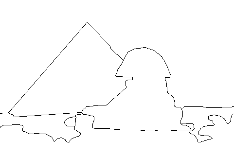
(c)

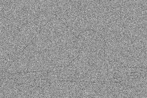
Figure 10: (a) An image from the BSD500. (b) Ground-truth contour map $B$ defined by the object boundaries traced by a human. (c) Real-valued image of noisy measurements $I$.

8.1.1 Scene Grammar

To specify a prior model for contour maps we use the PSG contour model defined by Grammar 3. This grammar is similar to Grammar 2 in Section 3.2, but with model parameters estimated from contour maps in the BSD500 training set.

The $\operatorname*{\mathsf{P}}$ bricks in a scene represent the trace of a set of curves in the image grid, and define a contour map $B$. That is, we set $B(i,j)=1$ iff $(\operatorname*{\mathsf{P}},(i,j))\in S$.

Note that a ground-truth contour map $B$ only specifies the set of $\operatorname*{\mathsf{P}}$ bricks in a scene. We do not have observations for the $\operatorname*{\mathsf{C}}$ bricks or the rules used to generate a scene. Therefore we used the approximate EM procedure described in Section 7 to estimate model parameters.

 

$\Sigma=\{\operatorname*{\mathsf{C}},\operatorname*{\mathsf{P}}\}$.

$\Omega_{\operatorname*{\mathsf{C}}}=[N]\times[M]\times[8]$.

$\Omega_{\operatorname*{\mathsf{P}}}=[N]\times[M]$.

Rules:

$\begin{array}[]{llll}0.647,&(\operatorname*{\mathsf{C}},(x,y,\theta))&\rightarrow&(\operatorname*{\mathsf{P}},\delta((x,y))),(\operatorname*{\mathsf{C}},\delta(((x,y)+\operatorname*{round}(T_{\theta}(1,0)),\theta))).\\ 0.147,&(\operatorname*{\mathsf{C}},(x,y,\theta))&\rightarrow&(\operatorname*{\mathsf{P}},\delta((x,y))),(\operatorname*{\mathsf{C}},\delta(((x,y)+\operatorname*{round}(T_{\theta-1}(1,0)),\theta))).\\ 0.152,&(\operatorname*{\mathsf{C}},(x,y,\theta))&\rightarrow&(\operatorname*{\mathsf{P}},\delta((x,y))),(\operatorname*{\mathsf{C}},\delta(((x,y)+\operatorname*{round}(T_{\theta+1}(1,0)),\theta))).\\ 0.019,&(\operatorname*{\mathsf{C}},(x,y,\theta))&\rightarrow&(\operatorname*{\mathsf{C}},\delta((x,y,\theta-1))).\\ 0.019,&(\operatorname*{\mathsf{C}},(x,y,\theta))&\rightarrow&(\operatorname*{\mathsf{C}},\delta((x,y,\theta+1))).\\ 0.012,&(\operatorname*{\mathsf{C}},(x,y,\theta))&\rightarrow&(\operatorname*{\mathsf{P}},\delta((x,y))).\\ 1.00,&(\operatorname*{\mathsf{P}},(x,y))&\rightarrow&\emptyset.\end{array}$

$\epsilon_{\operatorname*{\mathsf{C}}}=4.28\times 10^{-5}$,

$\epsilon_{\operatorname*{\mathsf{P}}}=1.87\times 10^{-12}$.

 

The function $T_{\theta}$ denotes a rotation in the plane by a discrete angle $\theta$ and $\operatorname*{round}$ maps a point in the plane to the nearest grid point.

Grammar 3: The PSG contour model (see Section 3.2). The model parameters were estimated using EM with contour maps from the BSD500.

8.1.2 Inference

To estimate $B$ from $I$ we incorporate the imaging model into the factor graph representation of the PSG contour model. We run LBP on this factor graph to compute conditional probabilities $p(B(i,j)=1\,|\,I)$.

Figure 11 shows the result of inference on several examples from the BSD500 test set. These results illustrate how we can recover good contour maps despite the ambiguous local observations.

By Bayes’ rule $p(S\,|\,I)\propto p(S)p(I\,|\,S)$. Recall that $B(i,j)=1$ iff $(\operatorname*{\mathsf{P}},(i,j))\in S$. In the factor graph $\mathcal{F}(\mathcal{G})$ there is a binary variable $X(\operatorname*{\mathsf{P}},(i,j))$ for each pixel $(i,j)$. We attach an additional unary factor to each of these variables, with potential $\Psi(x)=p_{x}(I(i,j))$. With these additional factors the graphical model represents the conditional distribution $p(S\,|\,I)$.

The factor graph representing the conditional distribution $P(S\,|\,I)$ for an $N$ by $M$ image has $O(NM)$ binary variables and $O(NM)$ edges. Therefore, using the approach in Section 5, one iteration of LBP takes $O(NM)$ time (linear in the size of the image). With our implementation of the PSG framework running LBP to convergence on a $481\times 321$ image took on average 1.5 hours.

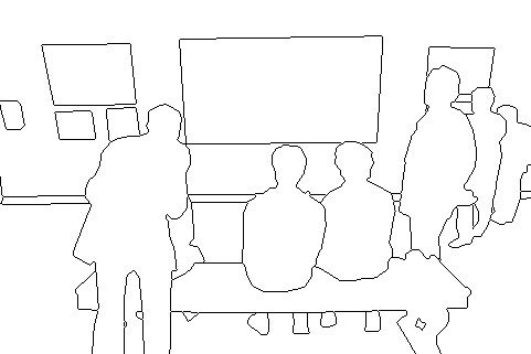
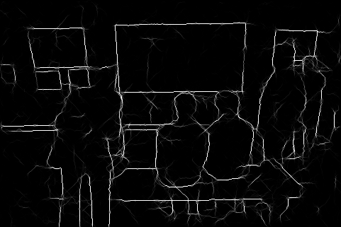
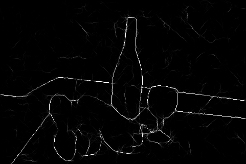
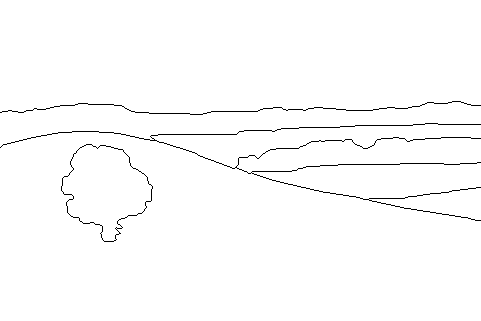
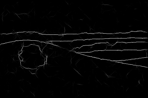
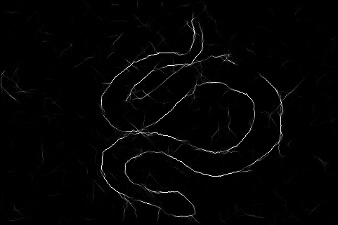
(a)	(b)	(c)

Figure 11: Contour detection results on four examples from the BSD500 test set. (a) Ground-truth contour maps $B$. (b) Noisy measurements $I$. (c) Estimated conditional probabilities $p(B(i,j)=1\,|\,I)$ with brighter values indicating a higher probability.

8.1.3 Quantitative Evaluation

For a quantitative evaluation we compare the result of thresholding the estimated conditional probabilities $p(B(i,j)=1\,|\,I)$ to the ground-truth contour maps. The results were evaluated using the 200 test images in the BSD500. Each threshold leads to a total number of correct (true positives) and incorrect (false positives) contour pixels detected, counted over all images in the test set.

Figure 12 shows the precision-recall curve obtained using different thresholds for detecting contour pixels, and also the results obtained with other methods in the same dataset. The figure also summarizes the area under the precision-recall curves (AUC) for each method.

To measure the importance of context for detecting contour pixels we evaluate a trivial PSG model with only the $\operatorname*{\mathsf{P}}$ bricks and the rule $\operatorname*{\mathsf{P}}\rightarrow\emptyset$. We refer to this model as the No-Context PSG.

We also include the results obtained with the Field-of-Patterns (FOP) models in [20]. The 1-level FOP model captures the statistics of 3x3 patterns in a binary image. The 4-level FOP model captures similar statistics of a multiscale representation of the image.

The quantitative results in Figure 12 indicate the importance of context for restoring binary contour maps. The evaluation also shows how the grammar based model and general inference method described in this paper lead to results that are comparable to state-of-the-art methods developed for this specific application.

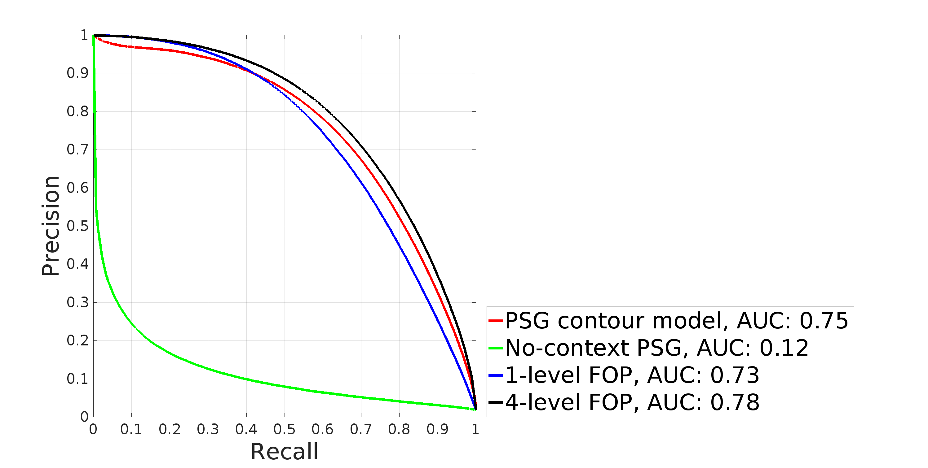
Figure 12: Precision-recall curves of different models for contour detection. The AUC numbers indicate the area under the curves.

8.2 Face Detection

Now we consider the problem of detecting faces and parts of faces in images. We use two datasets for the experiments with face detection:

1. Labeled Faces in the Wild (LFW) dataset: The LFW dataset was introduced in [29]. The dataset contains images with a single face. For the experiments in this section we randomly select $200$ images for training, and $100$ images for testing. We manually annotated each image with bounding box information for the face, left eye, right eye, nose, and mouth. Examples of labeled images are shown Figure 13.

2. Portraits dataset: To study face detection in more complex scenes, we use a dataset of $40$ images of family and class portraits collected from the Internet. We used the search strings “family portraits”, “class portraits” and “school portraits” on Google in November 2016 to collect images for the dataset. The images were manually annotated with bounding box information for each face, left eye, right eye, nose, and mouth. One example of a labeled image is shown in Figure 14. The average number of faces per image in the dataset is $5.9$.

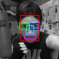
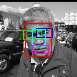
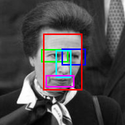
Figure 13: Examples of images in the LFW dataset. The images were annotated with bounding boxes for the face (red), left eye (green), right eye (blue), nose (cyan), and mouth (magenta).

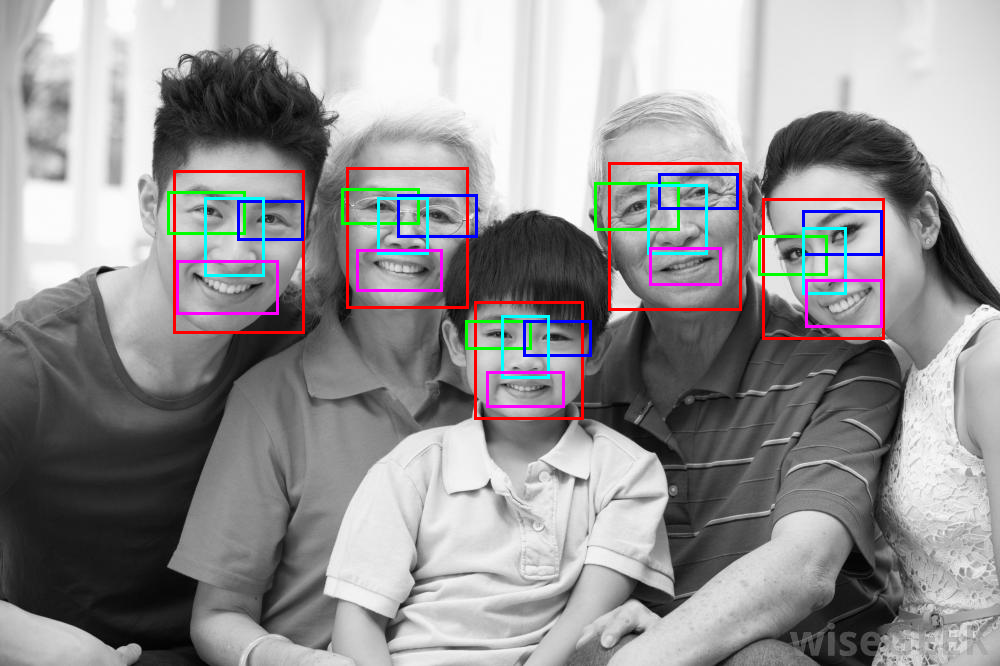
Figure 14: Example of an image in the Portraits dataset. The images were annotated with bounding boxes for each face (red), left eye (green), right eye (blue), nose (cyan), and mouth (magenta).

8.2.1 Face Detection Grammar

The PSG face model used in the face detection experiments is defined by Grammar 4. This model is similar to Grammar 1 in Section 3. However, the pose spaces in the model used here include scale information to represent objects of different sizes. The model used here also differentiates between parts of faces and objects that simply look like parts of faces but can appear outside the context of a face.

 

$\Sigma=\{\,\operatorname*{\mathsf{FACE}},\operatorname*{\mathsf{LEYE}},\operatorname*{\mathsf{REYE}},\operatorname*{\mathsf{NOSE}},\operatorname*{\mathsf{MOUTH}},\operatorname*{\mathsf{T-FACE}},\operatorname*{\mathsf{T-LEYE}},\operatorname*{\mathsf{T-REYE}},\operatorname*{\mathsf{T-NOSE}},\operatorname*{\mathsf{T-MOUTH}}\,\}$

$\forall A\in\Sigma,\;\Omega_{A}=\{\,(s,i,j)\mid s\in[L],\,(i,j)\in[N_{s}]\times[M_{s}]\,\}$.

Rules:

$\begin{array}[]{llll}1.0,&(\operatorname*{\mathsf{FACE}},\omega)&\rightarrow&(\operatorname*{\mathsf{T-FACE}},\delta(\omega)),\\ &&&(\operatorname*{\mathsf{LEYE}},\operatorname*{Categorical}(\theta_{1}(\omega))),\\ &&&(\operatorname*{\mathsf{REYE}},\operatorname*{Categorical}(\theta_{2}(\omega))),\\ &&&(\operatorname*{\mathsf{NOSE}},\operatorname*{Categorical}(\theta_{3}(\omega))),\\ &&&(\operatorname*{\mathsf{MOUTH}},\operatorname*{Categorical}(\theta_{4}(\omega))),\\ 1.0,&(\operatorname*{\mathsf{LEYE}},\omega)&\rightarrow&(\operatorname*{\mathsf{T-LEYE}},\delta(\omega))\\ 1.0,&(\operatorname*{\mathsf{REYE}},\omega)&\rightarrow&(\operatorname*{\mathsf{T-REYE}},\delta(\omega))\\ 1.0,&(\operatorname*{\mathsf{NOSE}},\omega)&\rightarrow&(\operatorname*{\mathsf{T-NOSE}},\delta(\omega))\\ 1.0,&(\operatorname*{\mathsf{MOUTH}},\omega)&\rightarrow&(\operatorname*{\mathsf{T-MOUTH}},\delta(\omega))\\ 1.0,&(\operatorname*{\mathsf{T-LEYE}},\omega)&\rightarrow&\emptyset\\ 1.0,&(\operatorname*{\mathsf{T-REYE}},\omega)&\rightarrow&\emptyset\\ 1.0,&(\operatorname*{\mathsf{T-NOSE}},\omega)&\rightarrow&\emptyset\\ 1.0,&(\operatorname*{\mathsf{T-MOUTH}},\omega)&\rightarrow&\emptyset\end{array}$

$\epsilon_{\operatorname*{\mathsf{FACE}}}=10^{-4}$

$\epsilon_{\operatorname*{\mathsf{LEYE}}}=\epsilon_{\operatorname*{\mathsf{REYE}}}=\epsilon_{\operatorname*{\mathsf{NOSE}}}=\epsilon_{\operatorname*{\mathsf{MOUTH}}}=10^{-12}$

$\epsilon_{\operatorname*{\mathsf{T-FACE}}}=\epsilon_{\operatorname*{\mathsf{T-LEYE}}}=\epsilon_{\operatorname*{\mathsf{T-REYE}}}=\epsilon_{\operatorname*{\mathsf{T-NOSE}}}=\epsilon_{\operatorname*{\mathsf{T-MOUTH}}}=10^{-4}$.

 

Grammar 4: The PSG face model. The grammar defines scenes with faces and parts of faces of different sizes. A pose $(s,i,j)$ specifies a size $s$ and a location $(i,j)$ in a grid. The parameters $\theta_{i}(\omega)$ define categorical distributions for the pose of a part relative to the pose of a face.

The PSG face model has a different symbol for each face part, including separate symbols for the left and right eyes. To model visual appearance of objects the grammar includes additional symbols that represent templates. A template symbol is denoted with the $\operatorname*{\mathsf{T-}}$ prefix. The set of template symbols is denoted by $\Sigma_{T}$.

Templates can appear either in the context of a face or in the background. This makes it possible to differentiate between an eye (nose, etc.) and an object that simply looks like an eye (nose, etc.). The distinction is important to supress false positive detections that arise from background clutter (see [7]). The parts of the face have very low self-rooting probability ($10^{-12}$) while the corresponding template symbols have a relatively higher self-rooting probability ($10^{-4}$). As a result, when objects appear out of context they are interpreted as a self-rooted template.

The poses in the PSG face model include position and scale information to capture objects of different sizes. The pose spaces are defined so that larger objects are localized with lower spatial resolution. This allows for representing objects of different sizes efficiently.

Let $L$, $K$, $N$, and $M$ be positive integers. For each $A\in\Sigma$ we have

$$\Omega_{A}=\{\,(s,i,j)\mid s\in[L],\,(i,j)\in[N_{s}]\times[M_{s}]\,\},$$

$$N_{s}=\left\lfloor\frac{N}{2^{s/K}}\right\rfloor,\;\;M_{s}=\left\lfloor\frac{M}{2^{s/K}}\right\rfloor.$$

A pose $(s,i,j)\in\Omega_{A}$ specifies a scale $s\in[L]$ and a position $(i,j)$ in a $N_{s}\times M_{s}$ grid. Objects in scale $s$ have size proportional to $2^{s/K}$ and are localized in a grid with spacing $2^{s/K}$. With this construction $|\Omega_{A}|=O(KNM)$, independent of $L$.

To represent object sizes accurately we use $K=8$ in all of our experiments. The value of $N$ and $M$ were defined by the width and height of an image image divided by the size of the local image features used for modeling the appearance of templates.

The conditional pose distributions for each part of a face in the PSG face model are categorical distributions with parameters $\theta_{i}(\omega)$ for $1\leq i\leq 4$. The pose distributions are defined using relative poses to impose scale and shift (translation) invariance. The distributions were estimated from the frequencies of relative positions and sizes between objects in the LFW training dataset.

The pose of an object specifies a location and scale, and we approximate the extent of the object by a rectangular box of varying size but with fixed aspect ratio. It is also possible to define objects using a collection of smaller parts, like corners and edges. In this case the location of the smaller parts can be used to compute a more accurate bounding box for the object.

8.2.2 Face Data Model

To define a data model we use templates that capture the appearance of local image features. For the experiments in this section we define template responses using histogram-of-gradient (HOG) features in a feature pyramid (see [11] and [17]).

We trained templates for each face part and a template for the whole face using the publicly-available code from [16]. The templates are trained to have positive responses on a set of positive examples and negative responses on a set of negative examples. We used the annotations in the LFW training set to define positive examples for each object type. The negative examples were taken from images in the PASCAL VOC 2012 dataset ([15]). Figure 15 shows the resulting HOG templates that were used for the experiments with face detection.

For a template symbol $A\in\Sigma_{T}$ let $H_{A}$ be a template associated with $A$ and $H_{A}(I,\omega)$ be the response of $H_{A}$ at the position and scale specified by $\omega$ within $I$. The data we use for inference of a scene $S$ is the collection of template responses,

$$H=\{H_{A}(\omega,I)\,|\,A\in\Sigma_{T},\omega\in\Omega_{A}\}.$$

To derive a tractable model for $p(H\,|\,S)$ we use the approach described in [23] to define a model for a family of local tests.

We assume the template responses are conditionally independent given $S$,

$$p(H\,|\,S)=\prod_{A\in\Sigma_{T}}\prod_{\omega\in\Omega_{A}}p(H_{A}(\omega,I)\,|\,S).$$

We also assume the conditional distributions $p(H_{A}(\omega,I)=v\,|\,S)$ depend only on whether or not $(A,\omega)$ is present in $S$,

$$p(H_{A}(\omega,I)=v\,|\,S)=\begin{cases}p_{A,0}(v)&(A,\omega)\not\in S,\\ p_{A,1}(v)&(A,\omega)\in S.\end{cases}$$

To estimate $p_{A,0}$ and $p_{A,1}$ we compute histograms of the template responses in positive and negative training examples of each object type. Figure 16 shows the estimated distributions of template responses for the various template symbols in the grammar.

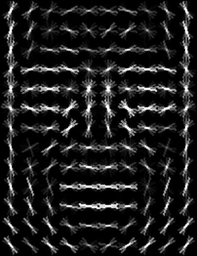
$\operatorname*{\mathsf{T-FACE}}$	$\operatorname*{\mathsf{T-LEYE}}$	$\operatorname*{\mathsf{T-REYE}}$	$\operatorname*{\mathsf{T-NOSE}}$	$\operatorname*{\mathsf{T-MOUTH}}$

Figure 15: Visualization of the HOG templates used for face detection. Note that the templates for the $\operatorname*{\mathsf{T-LEYE}}$ and $\operatorname*{\mathsf{T-REYE}}$ symbols are subtly different, indicating there is a visual difference between the two parts. Also note that the $\operatorname*{\mathsf{T-MOUTH}}$ template shares some similarities to both the $\operatorname*{\mathsf{T-LEYE}}$ and $\operatorname*{\mathsf{T-REYE}}$ filters.

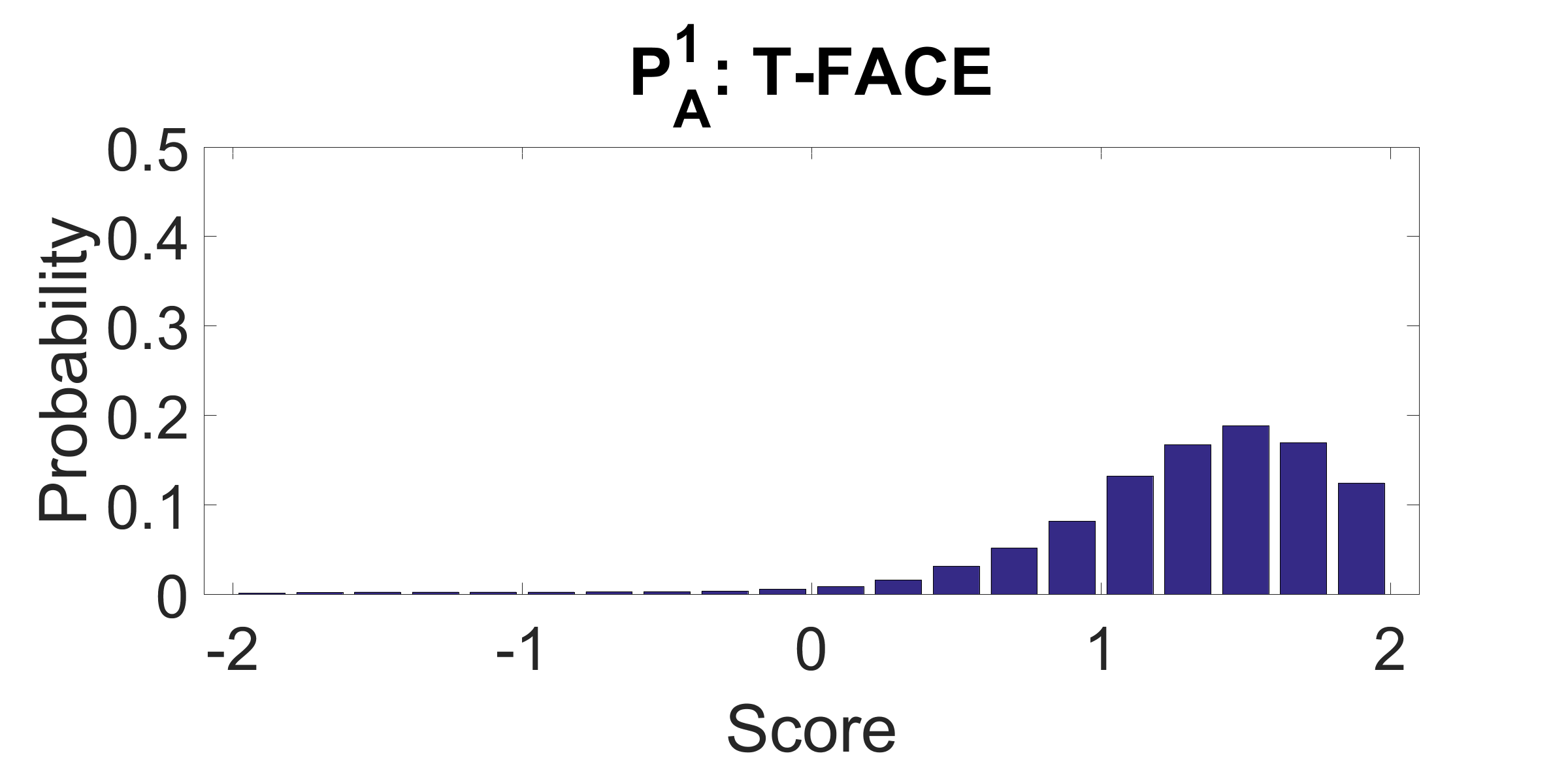
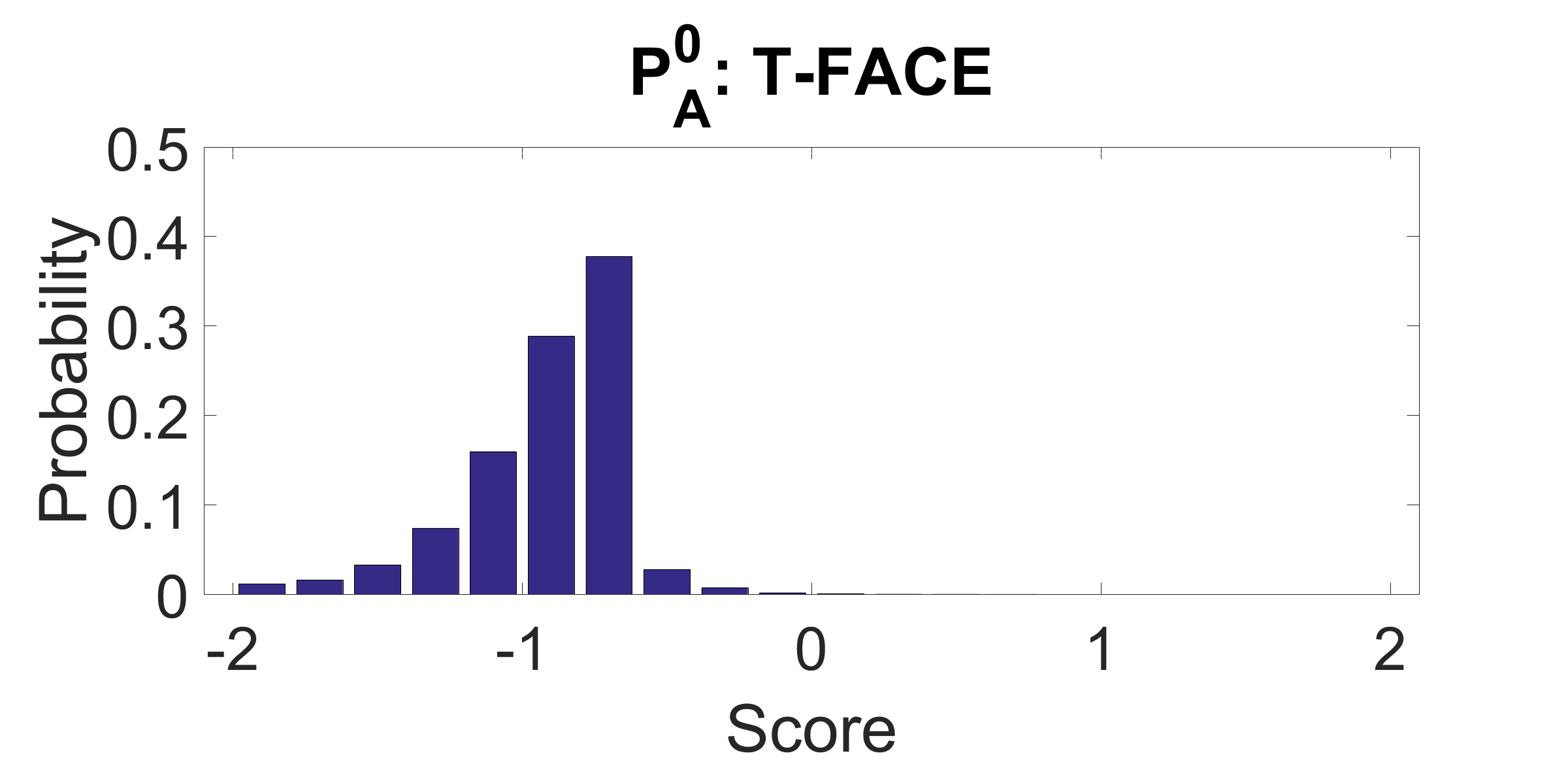
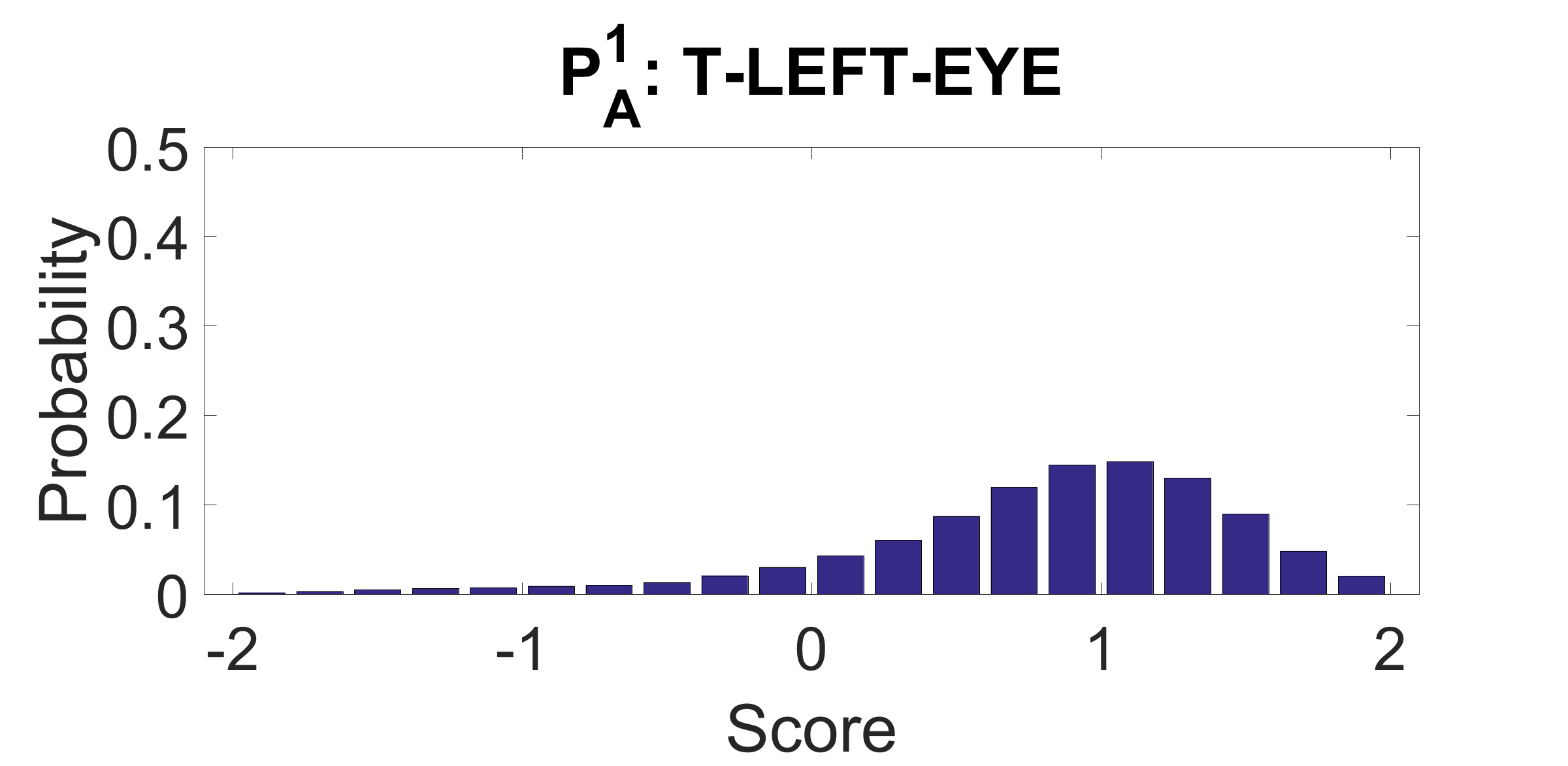
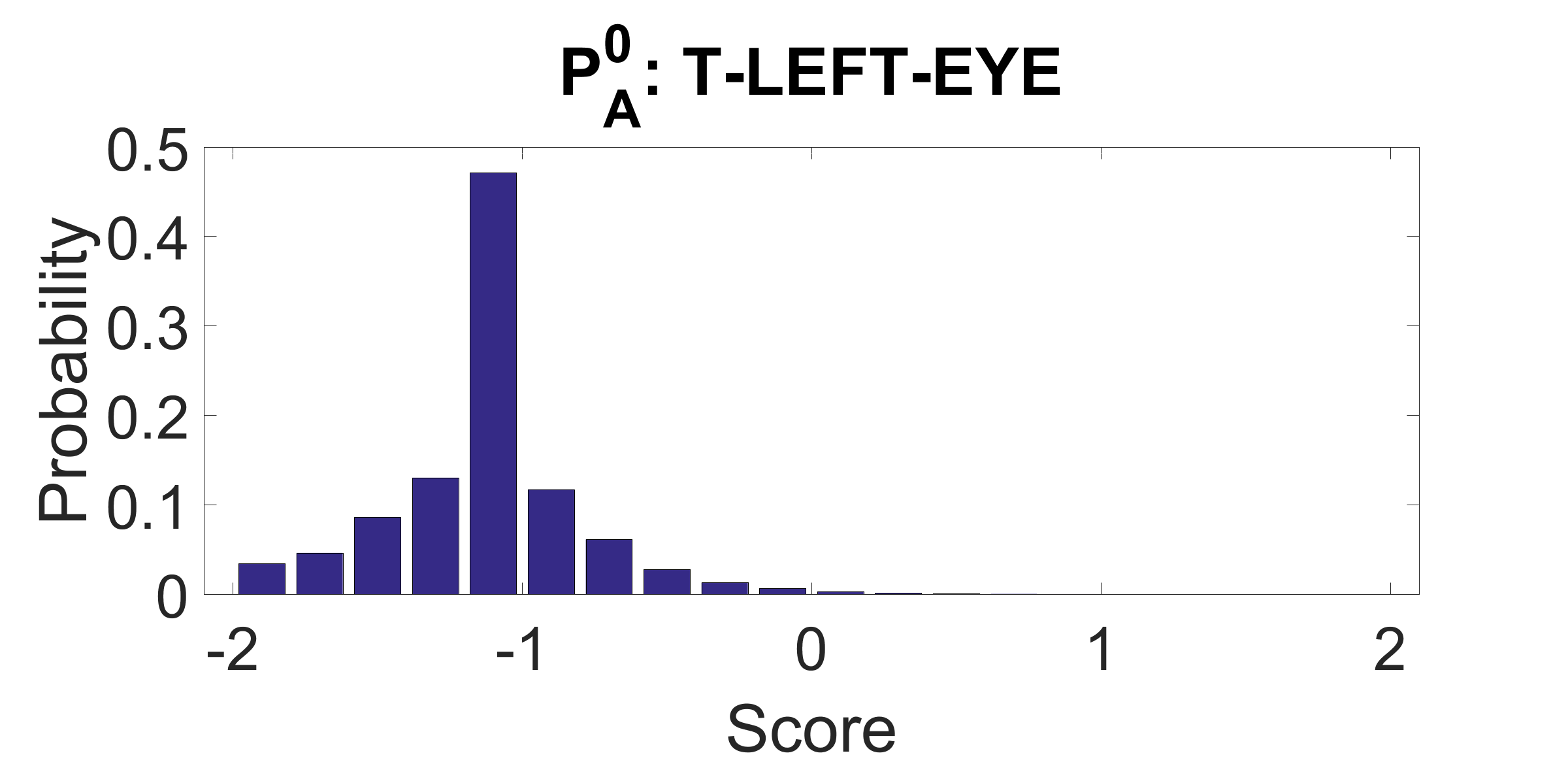
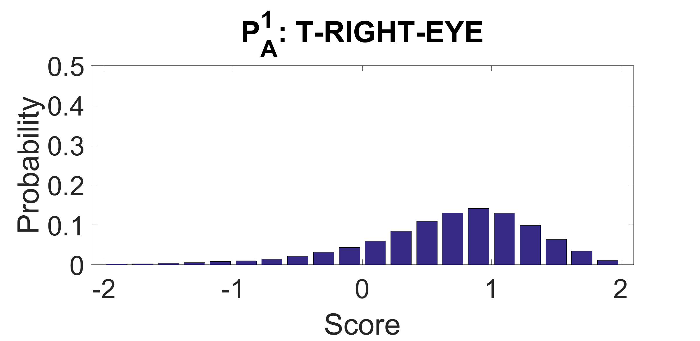
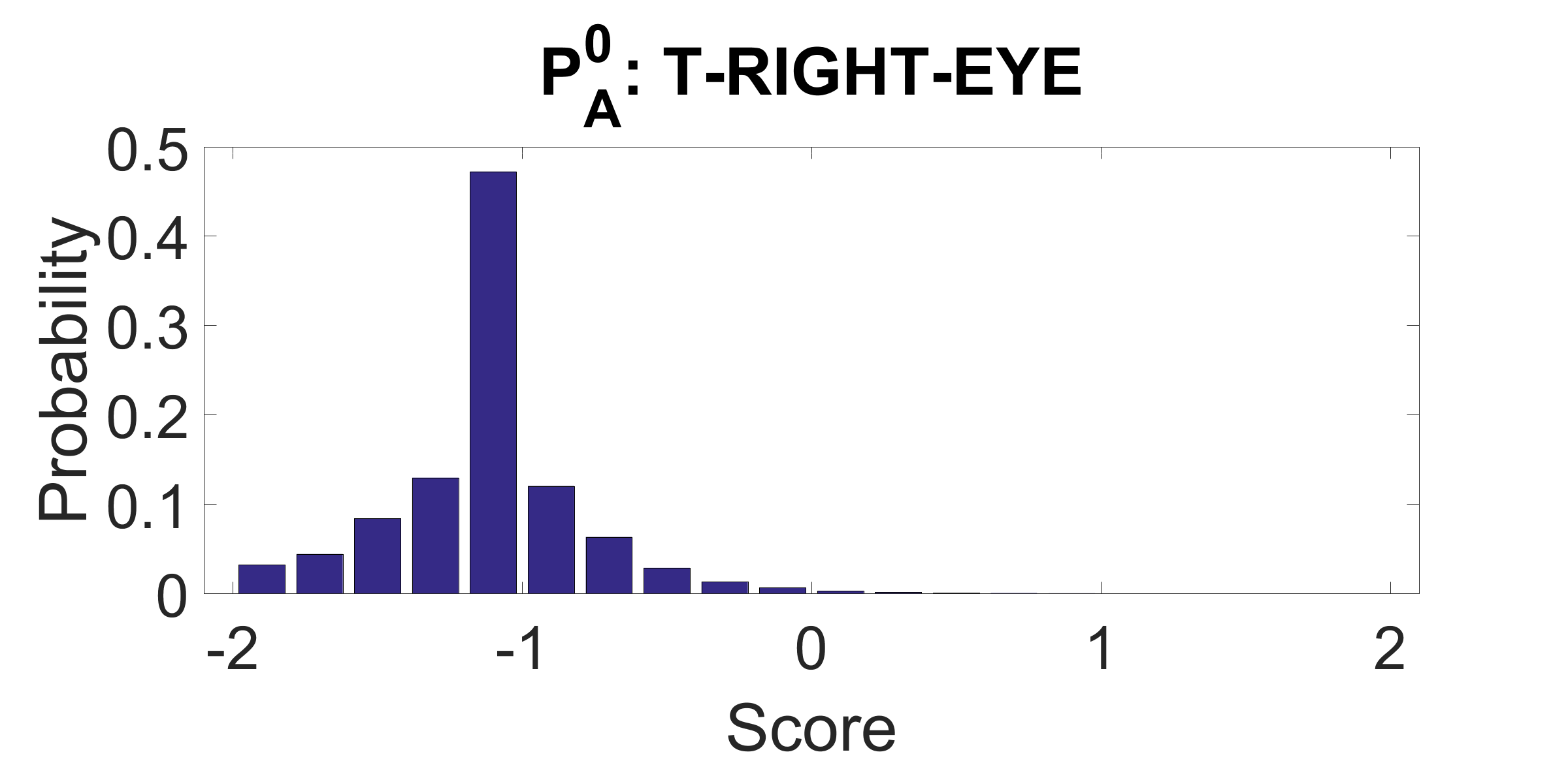
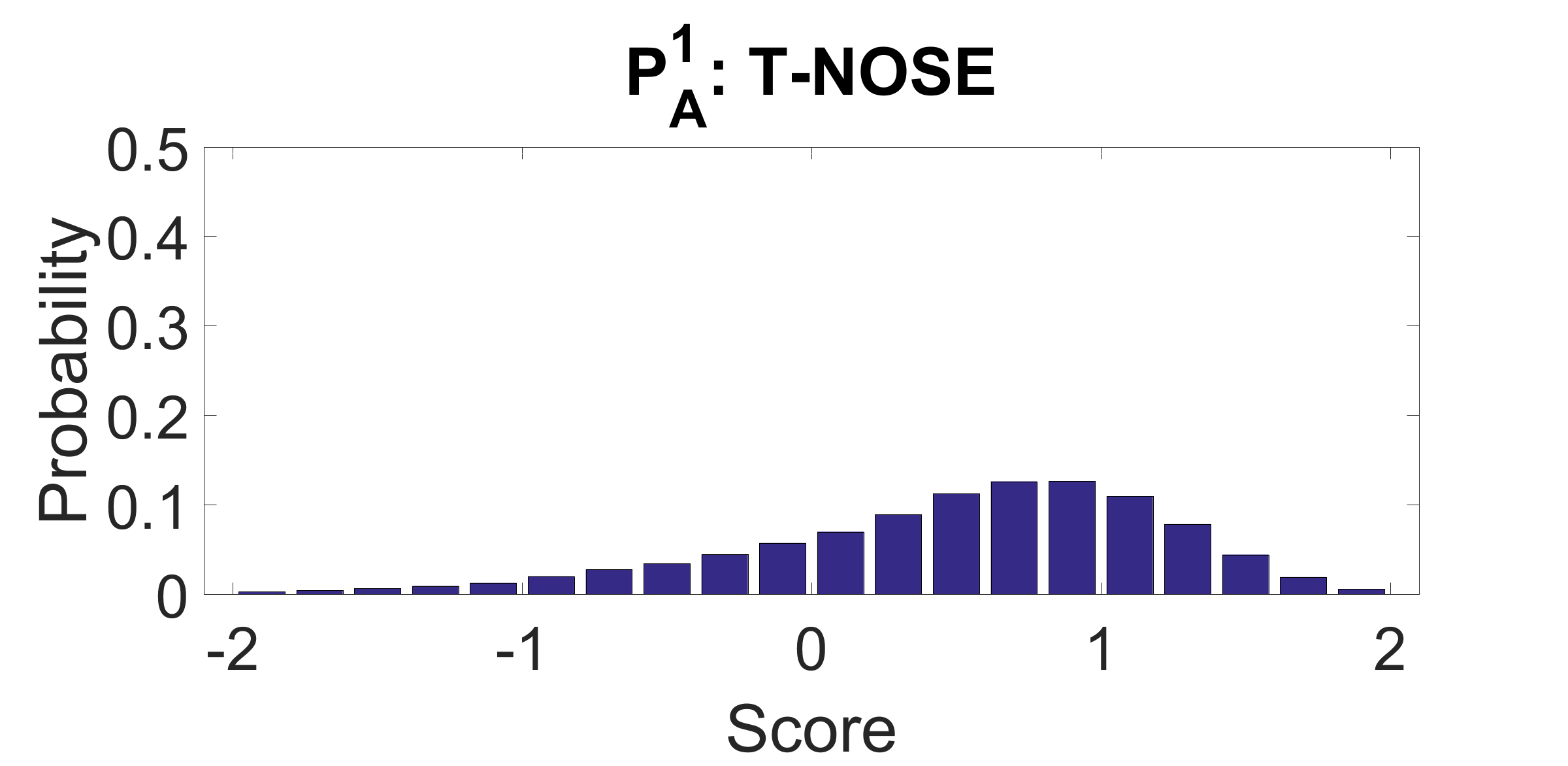
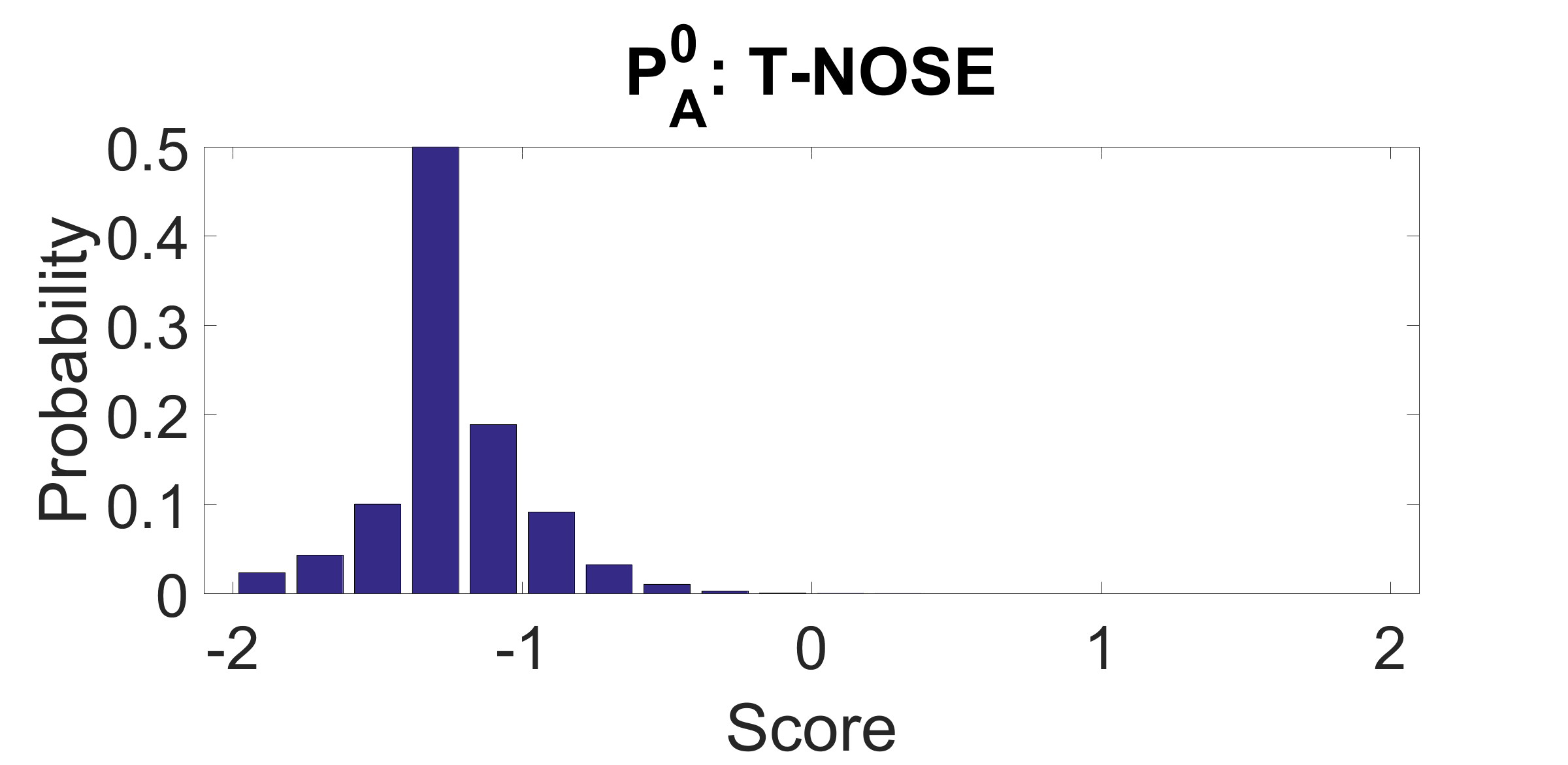
Figure 16: Distributions over template responses in the face data model. The first column shows the distribution of responses conditional on the presence of an object. The second column shows the distribution of responses in the background.

8.2.3 Inference

To detect objects in an image $I$ we consider the posterior $p(S\,|\,H)$. The probability that there is an object of type $A$ in pose $\omega$ is given by $p(X(A,\omega)=1\,|\,H)$.

By Bayes’ rule, $p(S\,|\,H)\propto p(S)p(H\,|\,S)$ and we incorporate $p(H\,|\,S)$ into the factor graph representation of $p(S)$ for posterior inference with LBP.

The factor graph $\mathcal{F}({\mathcal{G}})$ has a binary variable $X(A,\omega)$ for each $A\in\Sigma_{T}$ and $\omega\in\Omega_{A}$. We attach unary factors to these these variables with potential $\Psi(x)=p_{A,x}(H_{A}(\omega,I))$. With these additional factors the graphical model represents the conditional distribution $p(S\,|\,H)$.

8.2.4 Face Detection in the LFW Dataset

In the LFW dataset there is a single face in each image. To estimate the locations and sizes of the different objects (face and face parts) we simply select for each $A\in\{\,\operatorname*{\mathsf{FACE}},\operatorname*{\mathsf{REYE}},\operatorname*{\mathsf{LEYE}},\operatorname*{\mathsf{NOSE}},\operatorname*{\mathsf{MOUTH}}\,\}$ the pose

$$\omega_{A}^{*}=\operatorname*{arg\,max}_{\omega\in\Omega_{A}}\hat{p}(X(A,\omega)=1\,|\,H),$$

where $\hat{p}$ is the belief computed by LBP.

For comparison we also evaluate the results of using the templates to localize objects of each type independently. We refer to this method as the No-Context approach. In this case for each $A\in\{\,\operatorname*{\mathsf{T-FACE}},\operatorname*{\mathsf{T-LEYE}},\operatorname*{\mathsf{T-REYE}},\operatorname*{\mathsf{T-NOSE}},\operatorname*{\mathsf{T-MOUTH}}\,\}$ we select the pose

$$\omega_{A}^{*}=\operatorname*{arg\,max}_{\omega\in\Omega_{A}}\frac{p_{A,1}(H_{A}(\omega,I))}{p_{A,0}(H_{A}(\omega,I))}.$$

Figure 17 shows several results using both methods. Inference with the PSG face model correctly localized all parts in these images. On the other hand, inference with the No-Context approach leads to mistakes in three of the four images shown. These mistakes can be attributed to the visual similarity of the face parts, at least when represented using HOG features. We see that the context provided by the PSG face model resolves ambiguities and improves object localization.

Inference with the PSG face model took 120 seconds on a $250\times 250$ image. Inference with the No-Context model simply involves evaluating the template responses at every position and scale within the image, and took approximately 5 seconds per image.

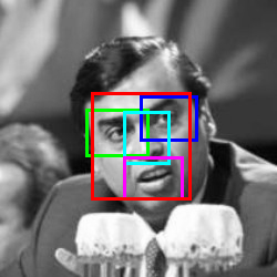
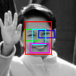
Ground Truth
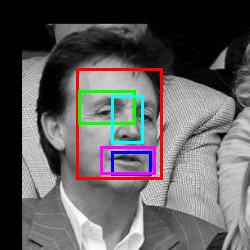
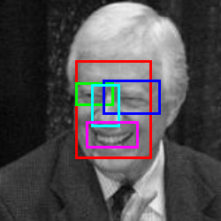
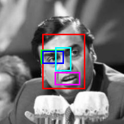
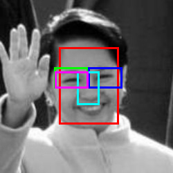
No-Context
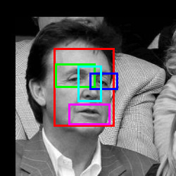
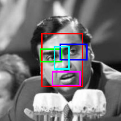
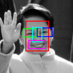
PSG face model

Figure 17: Localization results in the LFW dataset. The objects are $\operatorname*{\mathsf{FACE}}$ (red), $\operatorname*{\mathsf{LEYE}}$ (green), $\operatorname*{\mathsf{REYE}}$ (blue), $\operatorname*{\mathsf{NOSE}}$ (cyan), and $\operatorname*{\mathsf{MOUTH}}$ (magenta). The No-Context approach makes several mistakes due to the visual similarity between different parts. The PSG face model accurately localizes all objects in these examples.

Table 1 summarizes the localization accuracy obtained using the PSG face model and the No-Context approach in the LFW dataset. For comparison Table 1 also summarizes the results obtained using a pictorial structure model described in Section 8.2.6.

Model	$\operatorname*{\mathsf{FACE}}$	$\operatorname*{\mathsf{LEYE}}$	$\operatorname*{\mathsf{REYE}}$	$\operatorname*{\mathsf{NOSE}}$	$\operatorname*{\mathsf{MOUTH}}$	Average
No-Context model	3.7	4.7	8.2	3.3	13.6	6.7
PSG face model	3.5	2.6	3.3	2.4	3.5	3.1
Pictorial Structure	3.3	2.6	3.1	2.4	3.4	3.0

Table 1: Mean distance between predicted and ground truth object location on the LFW dataset. The locations are the centers of bounding boxes and distances were measured in pixels.

8.2.5 Face Detection on the Portraits Dataset

To study face detection in images with multiple faces we use the Portraits dataset described above. Figures 18 and 19 show several results obtained using the PSG face model and the No-Context approach. In each image we show the top $K$ poses for each object type, after performing non-maximum suppression, where $K$ is the number of faces in the image. As in the LFW dataset we see several mistakes in the No-Context results, while the results obtained with the PSG face model are almost perfect.

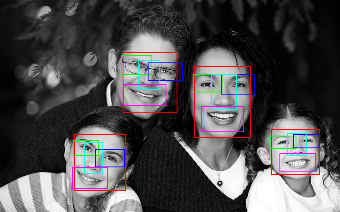
Ground Truth
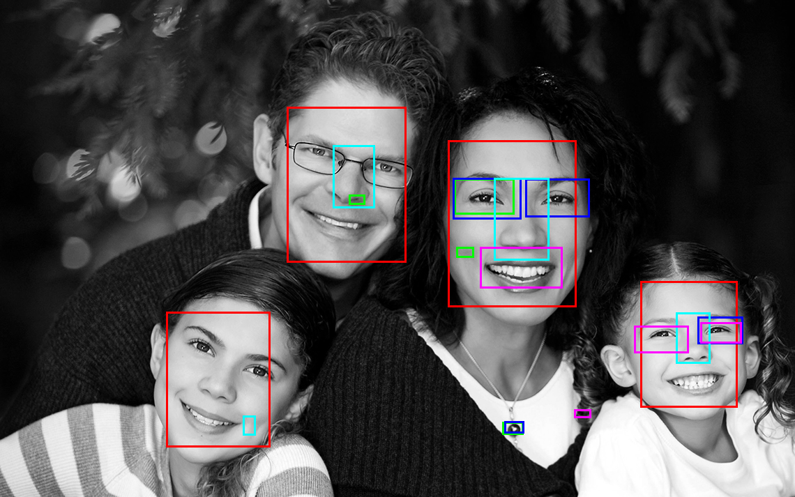
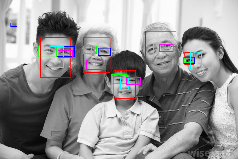
No-Context
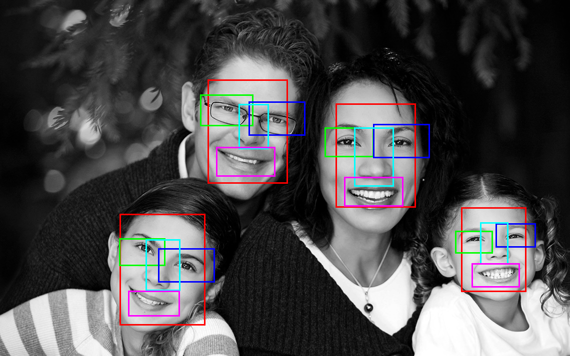
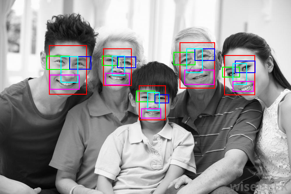
PSG face model

Figure 18: Top $K$ detections of each object type on two images from the Portraits dataset. The objects are $\operatorname*{\mathsf{FACE}}$ (red), $\operatorname*{\mathsf{LEYE}}$ (green), $\operatorname*{\mathsf{REYE}}$ (blue), $\operatorname*{\mathsf{NOSE}}$ (cyan), and $\operatorname*{\mathsf{MOUTH}}$ (magenta).

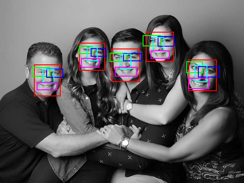
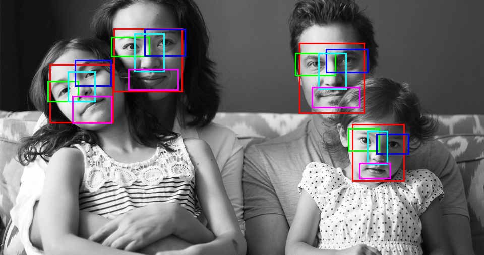
Ground Truth
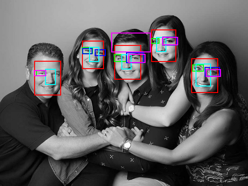
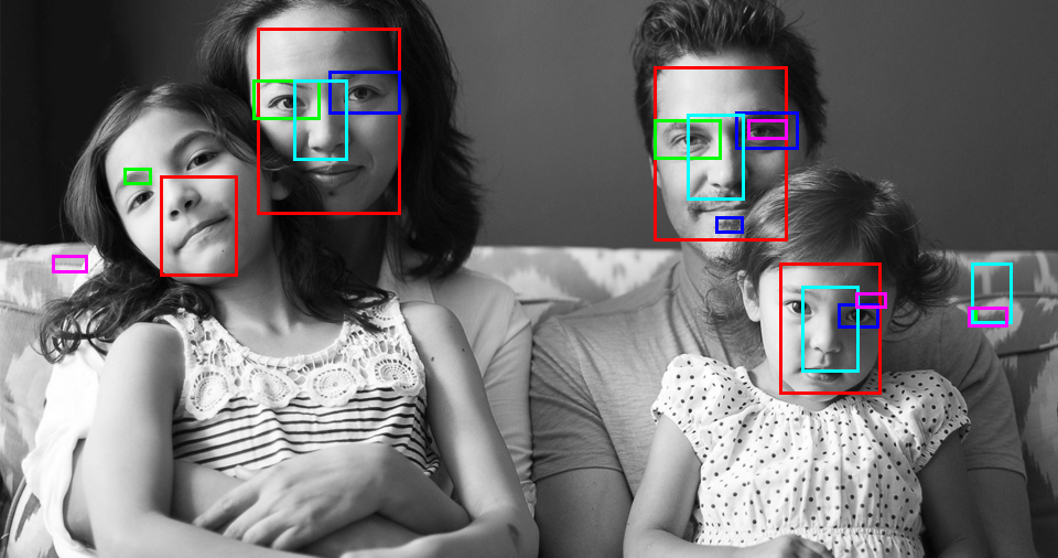
No-Context
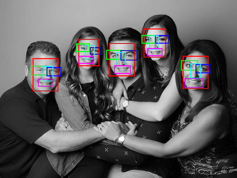
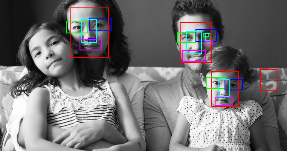
PSG face model

Figure 19: Top $K$ detections of each object type on two images from the Portraits dataset. The objects are $\operatorname*{\mathsf{FACE}}$ (red), $\operatorname*{\mathsf{LEYE}}$ (green), $\operatorname*{\mathsf{REYE}}$ (blue), $\operatorname*{\mathsf{NOSE}}$ (cyan), and $\operatorname*{\mathsf{MOUTH}}$ (magenta). The example on the right shows a difficult case where a face is significantly rotated, and the pattern on the couch resembles a face.

For a quantitative evaluation of the PSG face model when the number of faces in the image is unknown we generate a set of detections for each symbol by thresholding the estimated conditional probabilities $\hat{p}(X(A,\omega)=1\,|\,H)$ after non-maximum suppression.

For the No-Context model we generate detections by performing non-maximum suppression and thresholding the likelihood ratios $p_{A,1}(H_{A}(\omega,I))/p_{A,0}(H_{A}(\omega,I))$.

By considering different detection thresholds we obtain a precision-recall curve for each object type with each method. Table 2 summarizes the area under the precision-recall curves.

For comparison, Table 2 also summarizes the results obtained using a pictorial structure model described below and a PSG model with no face template. The performance of the PSG model without a face template is still quite good, including for detecting the face itself. This demonstrates how we can detect objects defined solely by their relationship to other objects.

Model	$\operatorname*{\mathsf{FACE}}$	$\operatorname*{\mathsf{LEYE}}$	$\operatorname*{\mathsf{REYE}}$	$\operatorname*{\mathsf{NOSE}}$	$\operatorname*{\mathsf{MOUTH}}$	Average
No-Context	0.95	0.50	0.48	0.90	0.32	0.63
PSG face model	0.97	0.81	0.81	0.96	0.80	0.87
PSG with no face template	0.93	0.78	0.80	0.95	0.76	0.84
Pictorial Structure	0.97	0.78	0.69	0.96	0.73	0.82

Table 2: Area under the precision-recall curves in the Portraits dataset.

8.2.6 Comparison to a Pictorial Structure model

The PSG face model is closely related to a pictorial structure model (see [18]). We obtain a pictorial structure model if we include an additional constraint that a scene has exactly one face and one set of corresponding face parts. With this constraint the posterior, $p(S\,|\,H)$, can be represented by a tree-structured graphical model. The graphical model has one variable for each face part connected to a variable for the face. The value of a variable specifies the pose of the corresponding object. For this tree-structure model we can compute exact posterior marginals using dynamic programming, following the approach in [18].

Tables 1 and 2 summarize results obtained using exact inference with a pictorial structure model for comparison with the PSG face model. To detect multiple objects of a single type in an image we threshold the probability of each pose after non-maximum suppression.

In the LFW dataset, where there is a single face in each image, the pictorial structure model and the PSG face model perform similarly. On the other hand, the PSG face model outperforms the pictorial structure model when detecting faces in the Portraits dataset. In this case we see an advantage to modeling scenes with a variable number of objects.

9 Summary

We described a general framework for knowledge representation and for scene understanding using probabilistic scene grammars and loopy belief propagation.

Probabilistic scene grammars can generate complex structures and capture regularities of scenes in a variety of settings. The approach we develop for inference involves the construction of large graphical models that represent distributions over regular scenes. We use loopy belief propagation for inference and derive techniques for implementing the sum-product algorithm in this setting. The resulting method is efficient, robust, and broadly applicable.

We also considered the problem of learning model parameters using maximum-likelihood estimation, both from fully observed and partially observed secenes.

The main contribution of our work is a mathematical and algorithmic foundation for probabilistic modeling of scenes and for scene understanding with grammar models. We demonstrate the feasibility of the approach with several examples. The experimental results show how the same framework and computational engine can be used to address different problems and lead to practical methods for inference.

The design of sophisticated grammars for different applications and the development of methods to learn the structure of scene grammars are important topics for future research.

Acknowledgments

We thank Stuart Geman, Basilis Gidas, Caroline Klivans and Jackson Loper for many helpful discussions about this research. We also thank the anonymous reviewers for many helpful comments that helped improve the presentation of this material. This material is based upon work supported by the National Science Foundation under Grant No. 1447413.

Appendix A Derivation of message passing formulas

Below we derive the expressions that are used in the efficient implementation of loopy belief propagation. We assume all messages are non-zero and are normalized to sum to one.

Note that if $\mu_{1}(x_{1}),\ldots,\mu_{n}(x_{n})$ are $n$ vectors that sum to one and $x=(x_{1},\ldots,x_{n})$, then

$$\sum_{x}\prod_{i}\mu_{i}(x_{i})=\prod_{i}\sum_{x_{i}}\mu_{i}(x_{i})=1.$$

*

Proof.

By definition,

$$\mu_{f\rightarrow Z}(\tau) = \kappa\sum_{y}\Psi^{L}_{\epsilon}(y,\tau)\prod_{i}\mu_{Y_{i}\rightarrow f}(y_{i}).$$ (4)

Consider the case $\tau=0$ and note that $\Psi^{L}_{\epsilon}(y,0)=0$ if $y\neq(0,\ldots,0)$.

$$\mu_{f\rightarrow Z}(0) = \kappa\sum_{y}\Psi^{L}_{\epsilon}(y,0)\prod_{i}\mu_{Y_{i}\rightarrow f}(y_{i}),$$ (5)

$$= \kappa(1-\epsilon)\prod_{i}\mu_{Y_{i}\rightarrow f}(0).$$ (6)

Now consider the case $\tau=1$.

$$\mu_{f\rightarrow Z}(1) = \kappa\sum_{y}\Psi^{L}_{\epsilon}(y,1)\prod_{i}\mu_{Y_{i}\rightarrow f}(y_{i}),$$ (7)

$$= \kappa\sum_{y}(1-\Psi^{L}_{\epsilon}(y,0))\prod_{i}\mu_{Y_{i}\rightarrow f}(y_{i}),$$ (8)

$$= \kappa\sum_{y}\prod_{i}\mu_{Y_{i}\rightarrow f}(y_{i})-\kappa\sum_{y}\Psi^{L}_{\epsilon}(y,0)\prod_{i}\mu_{Y_{i}\rightarrow f}(y_{i}),$$ (9)

$$= \kappa-\mu_{f\rightarrow Z}(0).$$ (10)

Setting $\kappa=1$ ensures $\sum_{\tau}\mu_{f\rightarrow Z}(\tau)=1$. ∎

*

Proof.

By definition,

$$\mu_{f\rightarrow Y_{i}}(\tau) = \kappa\sum_{\begin{subarray}{c}y\\ y_{i}=\tau\end{subarray}}\sum_{z}\Psi^{L}_{\epsilon}(y,z)\mu_{Z\rightarrow f}(z)\prod_{j\neq i}\mu_{Y_{j}\rightarrow f}(y_{j}).$$ (11)

Consider the case $\tau=0$.

$$\mu_{f\rightarrow Y_{i}}(0) = \kappa\sum_{\begin{subarray}{c}y\\ y_{i}=0,\\ c(y)=0\end{subarray}}\sum_{z}\Psi^{L}_{\epsilon}(y,z)\mu_{Z\rightarrow f}(z)\prod_{j\neq i}\mu_{Y_{j}\rightarrow f}(y_{j})$$ (15)

$$+\;\kappa\sum_{\begin{subarray}{c}y\\ y_{i}=0\\ c(y)>0\end{subarray}}\sum_{z}\Psi^{L}_{\epsilon}(y,z)\mu_{Z\rightarrow f}(z)\prod_{j\neq i}\mu_{Y_{j}\rightarrow f}(y_{j}),$$

$$= \kappa((1-\epsilon)\mu_{Z\rightarrow f}(0)+\epsilon\mu_{Z\rightarrow f}(1))\prod_{j\neq i}\mu_{Y_{j}\rightarrow f}(0)$$

$$+\;\kappa\sum_{\begin{subarray}{c}y\\ y_{i}=0\\ c(y)>0\end{subarray}}\mu_{Z\rightarrow f}(1)\prod_{j\neq i}\mu_{Y_{j}\rightarrow f}(y_{j}),$$

$$= \kappa((1-\epsilon)\mu_{Z\rightarrow f}(0)+\epsilon\mu_{Z\rightarrow f}(1))\prod_{j\neq i}\mu_{Y_{j}\rightarrow f}(0)$$

$$+\;\kappa\mu_{Z\rightarrow f}(1)((\sum_{\begin{subarray}{c}y\\ y_{i}=0\end{subarray}}\prod_{j\neq i}\mu_{Y_{j}\rightarrow f}(y_{j}))-\prod_{j\neq i}\mu_{Y_{j}\rightarrow f}(0)),$$

$$= \kappa((1-\epsilon)\mu_{Z\rightarrow f}(0)+\epsilon\mu_{Z\rightarrow f}(1))\prod_{j\neq i}\mu_{Y_{j}\rightarrow f}(0)$$

$$+\;\kappa\mu_{Z\rightarrow f}(1)(1-\prod_{j\neq i}\mu_{Y_{j}\rightarrow f}(0)),$$

$$= \kappa(\mu_{Z\rightarrow f}(1)+(1-\epsilon)(\mu_{Z\rightarrow f}(0)-\mu_{Z\rightarrow f}(1))\prod_{j\neq i}\mu_{Y_{j}\rightarrow f}(0)).$$ (16)

Now consider the case $\tau=1$:

$$\mu_{f\rightarrow Y_{i}}(1) = \kappa\sum_{\begin{subarray}{c}y\\ y_{i}=1\end{subarray}}\sum_{z}\Psi^{L}_{\epsilon}(y,z)\mu_{Z\rightarrow f}(z)\prod_{j\neq i}\mu_{Y_{j}\rightarrow f}(y_{j}),$$ (17)

$$= \kappa\sum_{\begin{subarray}{c}y\\ y_{i}=1\end{subarray}}\mu_{Z\rightarrow f}(1)\prod_{j\neq i}\mu_{Y_{j}\rightarrow f}(y_{j}),$$ (18)

$$= \kappa\mu_{Z\rightarrow f}(1).$$ (19)

∎

*

Proof.

By definition,

$$\mu_{f\rightarrow Y}(\tau) = \kappa\sum_{z}\Psi^{S}_{\theta}(\tau,z)\prod_{i}\mu_{Z_{i}\rightarrow f}(z_{i}).$$ (20)

Consider the case $\tau=0$ and note that $\Psi^{S}_{\theta}(0,z)=0$ if $z\neq(0,\ldots,0)$.

$$\mu_{f\rightarrow Y}(0) = \kappa\prod_{i}\mu_{Z_{i}\rightarrow f}(0).$$ (21)

Now consider the case $\tau=1$ and note that $\Psi^{S}_{\theta}(1,z)=0$ if $c(z)\neq 1$.

$$\mu_{f\rightarrow Y}(1) = \kappa\sum_{\begin{subarray}{c}z\\ c(z)=1\end{subarray}}\Psi^{S}_{\theta}(1,z)\prod_{i}\mu_{Z_{i}\rightarrow f}(z_{i}),$$ (22)

$$= \kappa\sum_{i}\theta_{i}\mu_{Z_{i}\rightarrow f}(1)\prod_{j\neq i}\mu_{Z_{j}\rightarrow f}(0),$$ (23)

$$= \kappa(\sum_{i}\theta_{i}\frac{\mu_{Z_{i}\rightarrow f}(1)}{\mu_{Z_{i}\rightarrow f}(0)})(\prod_{i}\mu_{Z_{j}\rightarrow f}(0)).$$ (24)

∎

*

Proof.

By definition,

$$\mu_{f\rightarrow Z_{i}}(\tau) = \kappa\sum_{\begin{subarray}{c}z\\ z_{i}=\tau\end{subarray}}\sum_{y}\Psi^{S}_{\theta}(y,z)\mu_{Y\rightarrow f}(y)\prod_{j\neq i}\mu_{Z_{j}\rightarrow f}(z_{j}).$$ (25)

Consider the case $\tau=0$.

$$\mu_{f\rightarrow Z_{i}}(0) = \kappa\sum_{\begin{subarray}{c}z\\ z_{i}=0\\ c(z)=0\end{subarray}}\sum_{y}\Psi^{S}_{\theta}(y,z)\mu_{Y\rightarrow f}(y)\prod_{j\neq i}\mu_{Z_{j}\rightarrow f}(z_{j})$$ (28)

$$+\;\kappa\sum_{\begin{subarray}{c}z\\ z_{i}=0\\ c(z)=1\end{subarray}}\sum_{y}\Psi^{S}_{\theta}(y,z)\mu_{Y\rightarrow f}(y)\prod_{j\neq i}\mu_{Z_{j}\rightarrow f}(z_{j}),$$

$$= \kappa\mu_{Y\rightarrow f}(0)\prod_{j\neq i}\mu_{Z_{j}\rightarrow f}(0)$$

$$+\;\kappa\sum_{\begin{subarray}{c}z\\ z_{i}=0\\ c(z)=1\end{subarray}}\Psi^{S}_{\theta}(1,z)\mu_{Y\rightarrow f}(1)\prod_{j\neq i}\mu_{Z_{j}\rightarrow f}(z_{j}),$$

$$= \kappa\mu_{Y\rightarrow f}(0)\prod_{j\neq i}\mu_{Z_{j}\rightarrow f}(0)$$

$$+\;\kappa\mu_{Y\rightarrow f}(1)(\sum_{j\neq i}\theta_{j}\frac{\mu_{Z_{j}\rightarrow f}(1)}{\mu_{Z_{j}\rightarrow f}(0)})(\prod_{j\neq i}\mu_{Z_{j}\rightarrow f}(0)).$$

Now consider the case $\tau=1$. Recall that $\Psi^{S}_{\theta}(y,z)=0$ if $c(z)>1$.

$$\mu_{f\rightarrow Z_{i}}(1) = \kappa\sum_{\begin{subarray}{c}z\\ z_{i}=1\\ c(z)=1\end{subarray}}\sum_{y}\Psi^{S}_{\theta}(y,z)\mu_{Y\rightarrow f}(y)\prod_{j\neq i}\mu_{Z_{j}\rightarrow f}(z_{j}),$$ (29)

$$= \kappa\theta_{i}\mu_{Y\rightarrow f}(1)\prod_{j\neq i}\mu_{Z_{j}\rightarrow f}(0).$$ (30)

∎

References

- [1] Alfred V. Aho, Ravi Sethi, and Jeffrey D. Ullman. Compilers: Principles, Tools, and Techniques. Addison-Wesley, 1986.
- [2] Yali Amit. 2D Object Detection and Recognition. MIT Press, 2002.
- [3] Pablo Arbelaez, Michael Maire, Charless Fowlkes, and Jitendra Malik. Contour detection and hierarchical image segmentation. IEEE Transactions on Pattern Analysis and Machine Intelligence, 33(5):898–916, May 2011.
- [4] Julian Besag. On the statistical analysis of dirty pictures. Journal of the Royal Statistical Society. Series B (Methodological), pages 259–302, 1986.
- [5] Elie Bienenstock, Stuart Geman, and Daniel Potter. Compositionality, MDL priors, and object recognition. In Advances in Neural Information Processing Systems, pages 838–844, 1997.
- [6] Michael Burl, Markus Weber, and Pietro Perona. A probabilistic approach to object recognition using local photometry and global geometry. In European Conference on Computer Vision, pages 628–641, 1998.
- [7] Lo-Bin Chang, Ya Jin, Wei Zhang, Eran Borenstein, and Stuart Geman. Context, computation, and optimal ROC performance in hierarchical models. International Journal of Computer Vision, 93(2):117–140, 2011.
- [8] Rama Chellapa and Anil Jain. Markov Random Fields: Theory and Application. Academic Press, 1993.
- [9] Noam Chomsky. Three models for the description of language. IRE Transactions on information theory, 2(3):113–124, 1956.
- [10] Thomas Cormen, Charles Leiserson, Ronald Rivest, and Clifford Stein. Introduction to algorithms second edition. The MIT Press, 2001.
- [11] Navneet Dalal and Bill Triggs. Histograms of oriented gradients for human detection. In IEEE Conference on Computer Vision and Pattern Recognition, pages 886–893, 2005.
- [12] A. P. Dempster, N. M. Laird, and D. B. Rubin. Maximum likelihood from incomplete data via the em algorithm. Journal of the Royal Statistical Society, Series B, 39(1):1–38, 1977.
- [13] Frank Drewes. Grammatical Picture Generation. Springer, 2006.
- [14] Richard Durbin, Sean R. Eddy, Anders Krogh, and Graeme Mitchison. Biological sequence analysis: probabilistic models of proteins and nucleic acids. Cambridge university press, 1998.
- [15] M. Everingham, L. Van Gool, C. K. I. Williams, J. Winn, and A. Zisserman. The PASCAL Visual Object Classes Challenge 2012 (VOC2012) Results, 2012.
- [16] Pedro F. Felzenszwalb, Ross B. Girshick, and David McAllester. Discriminatively trained deformable part models, release 4, 2010.
- [17] Pedro F. Felzenszwalb, Ross B. Girshick, David McAllester, and Deva Ramanan. Object detection with discriminatively trained part-based models. IEEE transactions on pattern analysis and machine intelligence, 32(9):1627–1645, 2010.
- [18] Pedro F. Felzenszwalb and Daniel P. Huttenlocher. Pictorial structures for object recognition. International Journal of Computer Vision, 61(1):55–79, 2005.
- [19] Pedro F. Felzenszwalb and David McAllester. Object detection grammars. Univerity of Chicago Computer Science Technical Report 2010-02, 2010.
- [20] Pedro F. Felzenszwalb and John G. Oberlin. Multiscale fields of patterns. In Advances in Neural Information Processing Systems, pages 82–90, 2014.
- [21] Martin A. Fischler and Robert A. Elschlager. The representation and matching of pictorial structures. IEEE Transactions on computers, (1):67–92, 1973.
- [22] King Sun Fu. Syntactic methods in pattern recognition. Elsevier, 1974.
- [23] Donald Geman and Bruno Jedynak. An active testing model for tracking roads in satellite images. IEEE Transactions on Pattern Analysis and Machine Intelligence, 18(1):1–14, 1996.
- [24] Stuart Geman and Donald Geman. Stochastic relaxation, gibbs distributions, and the bayesian restoration of images. IEEE Transactions on Pattern Analysis and Machine Intelligence, 6:721–741, 1984.
- [25] Stuart Geman, Daniel F. Potter, and Zhiyi Chi. Composition systems. Quarterly of Applied Mathematics, 60(4):707–736, 2002.
- [26] Ulf Grenander. General Pattern Theory. Oxford University Press, 1993.
- [27] Matthew T. Harrison. Discovering compositional structures. PhD thesis, Brown University, 2005.
- [28] Tom Heskes, Onno Zoeter, and Wim Wiegerinck. Approximate expectation maximization. In Advances in Neural Information Processing Systems 16, pages 353–360, 2004.
- [29] Gary B. Huang, Manu Ramesh, Tamara Berg, and Erik Learned-Miller. Labeled faces in the wild: A database for studying face recognition in unconstrained environments. Technical Report 07-49, University of Massachusetts, Amherst, October 2007.
- [30] Ya Jin and Stuart Geman. Context and hierarchy in a probabilistic image model. In IEEE Conference on Computer Vision and Pattern Recognition, volume 2, pages 2145–2152, 2006.
- [31] Dan Klein. The Unsupervised Learning of Natural Language Structure. PhD thesis, Stanford University, 2005.
- [32] Frank R. Kschischang, Brendan J. Frey, and Hans-Andrea Loeliger. Factor graphs and the sum-product algorithm. IEEE Transactions on Information Theory, 47(2):498–519, 2001.
- [33] Tejas D Kulkarni, Pushmeet Kohli, Joshua B Tenenbaum, and Vikash Mansinghka. Picture: A probabilistic programming language for scene perception. In IEEE Conference on Computer Vision and Pattern Recognition, pages 4390–4399, 2015.
- [34] Christopher D. Manning and Hinrich Schütze. Foundations of statistical natural language processing. MIT Press, 1999.
- [35] David Mumford. The bayesian rationale for energy functionals. Geometry-driven diffusion in Computer Vision, pages 141–153, 1994.
- [36] David Mumford. Elastica and computer vision. In Algebraic geometry and its applications, pages 491–506. Springer, 1994.
- [37] Kevin P. Murphy, Yair Weiss, and Michael I. Jordan. Loopy belief propagation for approximate inference: An empirical study. In Uncertainty in Artificial Intelligence, pages 467–475, 1999.
- [38] Stephen E. Palmer. Vision science: Photons to phenomenology. MIT press, 1999.
- [39] Judea Pearl. Probabilistic reasoning in intelligent systems: networks of plausible inference. Morgan Kaufmann, 1988.
- [40] Przemyslaw Prusinkiewicz and Aristid Lindenmayer. The algorithmic beauty of plants (The Virtual Laboratory). Springer, 1991.
- [41] Azriel Rosenfeld. Picture Languages (Formal Models for Picture Recognition). Academic Press, 1979.
- [42] A. Shashua and S. Ullman. Structural saliency: The detection of globally salient structures using a locally connected network. MIT AI Lab Memo No. 1061, 1988.
- [43] Andreas Stolcke. Bayesian Learning of Probabilistic Language Models. PhD thesis, University of California at Berkeley, 1994.
- [44] Daniel Tarlow, Kevin Swersky, Richard S. Zemel, Ryan Prescott Adams, and Brendan J. Frey. Fast exact inference for recursive cardinality models. In Uncertainty in Artificial Intelligence, 2012.
- [45] Dustin Tran, Matthew D. Hoffman, Rif A. Saurous, Eugene Brevdo, Kevin Murphy, and David M. Blei. Deep probabilistic programming. In International Conference on Learning Representations, 2017.
- [46] Zhuowen Tu, Xiangrong Chen, Alan L. Yuille, and Song-Chun Zhu. Image parsing: Unifying segmentation, detection, and recognition. International Journal of Computer Vision, 63(2):113–140, 2005.
- [47] Martin J. Wainwright and Michael I. Jordan. Graphical models, exponential families, and variational inference. Foundations and Trends in Machine Learning, 1(1–2):1–305, 2008.
- [48] Yair Weiss. Correctness of local probability propagation in graphical models with loops. Neural computation, 12(1):1–41, 2000.
- [49] Lance R. Williams and David W. Jacobs. Stochastic completion fields: A neural model of illusory contour shape and salience. Neural computation, 9(4):837–858, 1997.
- [50] Jonathan S. Yedidia, William T. Freeman, and Yair Weiss. Understanding belief propagation and its generalizations. In Exploring artificial intelligence in the new millennium, pages 236–239. Morgan Kaufmann, 2001.
- [51] Yibiao Zhao and Song-Chun Zhu. Image parsing with stochastic scene grammar. In Advances in Neural Information Processing Systems, pages 73–81, 2011.
- [52] Long Zhu, Yuanhao Chen, and Alan Yuille. Unsupervised learning of probabilistic grammar-markov models for object categories. IEEE Transactions on Pattern Analysis and Machine Intelligence, 31(1):114–128, 2009.
- [53] Song-Chun Zhu and David Mumford. A stochastic grammar of images. Foundations and Trends in Computer Graphics and Vision, 2(4):259–362, 2007.