Geometrical symmetries of nuclear systems: ${\cal D}_{3h}$ and ${\cal T}_{d}$ symmetries in light nuclei

Abstract

The role of discrete (or point-group) symmetries in $\alpha$-cluster nuclei is discussed in the framework of the algebraic cluster model which describes the relative motion of the $\alpha$-particles. Particular attention is paid to the discrete symmetry of the geometric arrangement of the $\alpha$-particles, and the consequences for the structure of the corresponding rotational bands. The method is applied to study cluster states in the nuclei ¹²C and ¹⁶O. The observed level sequences can be understood in a simple way as a consequence of the underlying discrete symmetry that characterizes the geometrical configuration of the $\alpha$-particles, i.e. an equilateral triangle with ${\cal D}_{3h}$ symmetry for ¹²C, and a tetrahedron with ${\cal T}_{d}$ symmetry for ¹⁶O. The structure of rotational bands provides a fingerprint of the underlying geometrical configuration of $\alpha$-particles.

Keywords: Alpha-cluster nuclei, geometrical symmetries, algebraic cluster model, energy spectrum, electromagnetic form factors, $B(EL)$ values

1 Introduction

The concept of symmetries has played an important role in nuclear structure physics, both continuous and discrete symmetries. Examples of continuous symmetries are isospin symmetry [1], Wigner’s combined spin-isospin symmetry [2], the (generalized) seniority scheme [3, 4], the Elliott model [5] and the interacting boson model [6]. In addition to providing simple analytic solutions which can be used to analyze and interpret the structure of nuclei, symmetries play a crucial role in establishing the connection between different models of nuclear structure, such as the spherical shell model of Goeppert-Mayer [7] and Jensen [8], the geometric collective model of Bohr and Mottelson [9] and the interacting boson model of Arima and Iachello [6]. In particular, the Elliott $SU(3)$ model provides a link between the spherical shell model and the quadrupole deformation of the geometric collective model, and the dynamical symmetries of the interacting boson model correspond to the harmonic vibrator, axial rotor and $\gamma$-unstable rotor limits of the geometric collective model. An recent review of the relation between symmetries of the spherical shell model and quadrupole and octupole deformations of the collective model can be found in Ref. [10].

On the other hand, discrete symmetries have been used in the context of collective models to characterize the intrinsic shape of the nucleus, such as axial symmetry for quadrupole deformations [9], and tetrahedral [11] and octahedral [11, 12] symmetries for deformations of higher multipoles. A different application is found in the context of $\alpha$-particle clustering in light nuclei to describe the geometric configuration of the $\alpha$ particles. Early work on $\alpha$-cluster models goes back to the 1930’s with studies by Wheeler [13], and Hafstad and Teller [14], followed by later work by Brink [15, 16] and Robson [17]. Recently, there has been a lot of renewed interest in the structure of $\alpha$-cluster nuclei, especially for the nucleus ¹²C [18]. The measurement of new rotational excitations of the ground state [19, 20] and the Hoyle state [21, 22, 23, 24] has stimulated a large theoretical effort to understand the structure of ¹²C ranging from studies based on the semi-microscopic algebraic cluster model [25], antisymmetrized molecular dynamics [26], fermionic molecular dynamics [27], BEC-like cluster model [28], ab initio no-core shell model [29], lattice effective field theory [30], no-core symplectic model [31], and the algebraic cluster model (ACM) [20, 32, 33]. A recent review on the structure of ¹²C can be found in Ref. [18].

It is the aim of this contribution to discuss the ACM for two-, three- and four-body clusters, and study possible applications in $\alpha$-cluster nuclei, like ⁸Be, ¹²C and ¹⁶O. In these applications, it is important to take into account the permutation symmetry between the identical $\alpha$ clusters. The manuscript is organized as follows. In Section 2 the radiation problem of various configurations of identical charged particles is discussed at the classical level. In Sections 3 and 4 some general properties of the ACM are presented which are relevant for two-, three- and four-body identical clusters, such as the structure of the Hamiltonian, permutation and geometrical symmetries, the classical limit, electromagnetic couplings, dynamical symmetries and shape-phase transitions. In the next three sections, the ACM for two-, three- and four-body clusters is developed in more detail. Particular attention is paid to the cases of the axial rotor, the oblate top and the spherical top, and their respective point group symmetries. Even though these special solutions do not correspond to a dynamical symmetry of the Hamiltonian, approximate formula for energies, form factors and electromagnetic transition rates can be derived in a semi-classical mean-field analysis. Finally, I discuss applications of the ACM to the cluster states in the nuclei ¹²C and ¹⁶O.

2 Classical treatment

In order to appreciate the effect of the geometric configuration of a number of identical charges (without magnetic moment, as in the case for the $\alpha$-particle model) on the multipole radiation, first consider the classical radiation problem for a charge distribution $\rho(\vec{r})$ with multipole moments

$$Q_{\lambda\mu}=\int r^{l}\,Y_{\lambda\mu}(\theta,\phi)\,\rho(\vec{r})\,d\vec{r}~{}.$$ (1)

From these multipole moments, the transition probability per unit time can be calculated as [34]

$$T(E\lambda)=\frac{8\pi c}{\hbar c}\,\frac{\lambda+1}{\lambda\left[(2\lambda+1)!!\right]^{2}}\,k^{2\lambda+1}\,B(E\lambda)~{},$$ (2)

with

$$B(E\lambda)=\sum_{\mu=-\lambda}^{\lambda}Q_{\lambda\mu}^{\ast}Q_{\lambda\mu}~{}.$$ (3)

For a point-like charge distribution of $k$ identical charges with coordinates $\vec{r}_{i}=(r_{i},\theta_{i},\phi_{i})$ ($i=1,\ldots,k$) the charge distribution is given by

$$\rho(\vec{r})=\frac{Ze}{k}\sum_{i=1}^{k}\delta(\vec{r}-\vec{r}_{i})~{}.$$ (4)

The corresponding $B(E\lambda)$ values are given by

$$B(E\lambda)=\left(\frac{Ze}{k}\right)^{2}\frac{2\lambda+1}{4\pi}\sum_{i,j=1}^{k}(r_{i}r_{j})^{\lambda}P_{\lambda}(\cos\theta_{ij})~{},$$ (5)

where $\theta_{ij}$ denotes the relative angle between the vectors $\vec{r}_{i}$ and $\vec{r}_{j}$

$$\cos\theta_{ij}=\cos\theta_{i}\cos\theta_{j}+\sin\theta_{i}\sin\theta_{j}\cos(\phi_{i}-\phi_{j})~{}.$$ (6)

For two-body clusters ($k=2$), the coordinates of the two $\alpha$ particles are taken with respect to the center of mass: $(r_{1},\theta_{1},\phi_{1})=(\beta,0,-)$ and $(r_{2},\theta_{2},\phi_{2})=(\beta,\pi,-)$ (see Fig. 1). The corresponding $B(E\lambda)$ values are

$$B(E\lambda)=\left(\frac{Ze\beta^{\lambda}}{2}\right)^{2}\frac{2\lambda+1}{4\pi}\left[2+2P_{\lambda}(-1)\right]~{},$$ (7)

which vanish for the odd multipoles, and are equal to

$$B(E\lambda)=\left(Ze\beta^{\lambda}\right)^{2}\,\frac{2\lambda+1}{4\pi}~{},$$ (8)

for the even multipoles.

Figure 1: Geometry of a two-, three- and four-body system

Next consider the case of three identical particles at the vertices of an equilateral triangle (point-group symmetry ${\cal D}_{3h}$) (see Fig. 1). The origin is placed at the center of mass so that the distance from the center is the same for all three particles $r_{i}=\beta$. The spherical coordinates of the three particles $\vec{r}_{i}=(r_{i},\theta_{i},\phi_{i})$ can be taken as $(\beta,0,-)$, $(\beta,2\pi/3,0)$ and $(\beta,2\pi/3,\pi)$ for $i=1,2$ and $3$, respectively, such that the relative angles $\cos\theta_{ij}=-1/2$ for all $i\neq j$. For this configuration, the multipole radiation is given by

$$B(E\lambda)=\left(\frac{Ze\beta^{\lambda}}{3}\right)^{2}\frac{2\lambda+1}{4\pi}\left[3+6P_{\lambda}(-\frac{1}{2})\right]~{},$$ (9)

which gives

$$B(E1) = 0~{},$$ (10a)

$$B(E2) = (Ze)^{2}\,\frac{5}{4\pi}\,\frac{1}{4}\,\beta^{4}~{},$$ (10b)

$$B(E3) = (Ze)^{2}\,\frac{7}{4\pi}\,\frac{5}{8}\,\beta^{6}~{},$$ (10c)

$$B(E4) = (Ze)^{2}\,\frac{9}{4\pi}\,\frac{9}{64}\,\beta^{8}~{},$$ (10d)

$$B(E5) = (Ze)^{2}\,\frac{11}{4\pi}\,\frac{35}{128}\,\beta^{10}~{},$$ (10e)

$$B(E6) = (Ze)^{2}\,\frac{13}{4\pi}\,\frac{281}{512}\,\beta^{12}~{}.$$ (10f)

The dipole radiation $B(E1)$ vanishes because of the spatial symmetry of the charge distribution.

Finally, consider the case of four identical particles at the vertices of a tetrahedron (point-group symmetry ${\cal T}_{d}$) (see Fig. 1). Again, the origin is placed at the center of mass so that the distance from the center is the same for all four particles $r_{i}=\beta$. The spherical coordinates of the three particles $\vec{r}_{i}=(r_{i},\theta_{i},\phi_{i})$ can be taken as $(\beta,0,-)$, $(\beta,\theta,0)$, $(\beta,\theta,2\pi/3)$ and $(\beta,\theta,4\pi/3)$, respectively, such that the relative angles satisfies $\cos\theta_{ij}=-1/3$ for all $i\neq j$. For this configuration, the multipole radiation is given by

$$B(E\lambda)=\left(\frac{Ze\beta^{\lambda}}{4}\right)^{2}\frac{2\lambda+1}{4\pi}\left[4+12P_{\lambda}(-\frac{1}{3})\right]~{},$$ (10k)

with

$$B(E1) = 0~{},$$ (10la)

$$B(E2) = 0~{},$$ (10lb)

$$B(E3) = (Ze)^{2}\frac{7}{4\pi}\frac{5}{9}\beta^{6}~{},$$ (10lc)

$$B(E4) = (Ze)^{2}\frac{9}{4\pi}\frac{7}{27}\beta^{8}~{},$$ (10ld)

$$B(E5) = 0~{},$$ (10le)

$$B(E6) = (Ze)^{2}\frac{13}{4\pi}\frac{32}{81}\beta^{12}~{}.$$ (10lf)

In this case, the multipoles with $\lambda=1$, $2$ and $5$ vanish as a consequence of the tetrahedral symmetry of the configuration of four $\alpha$ particles.

3 Algebraic cluster model

Algebraic models have found useful applications both in many-body and in few-body systems. Algebraic methods are based on the general criterion to introduce a $U(\nu+1)$ spectrum generating algebra for a bound-state problem with $\nu$ degrees of freedom. Well-known examples are the $U(6)$ interacting boson model for the $\nu=5$ quadrupole degrees of freedom in collective nuclei [6], and the $U(4)$ vibron model for the $\nu=3$ dipole degrees of freedom in diatomic molecules [35].

In this section, I briefly review the basic ingredients of the algebraic cluster model (ACM) which was introduced to describe the relative motion of cluster systems [32]. The relevant degrees of freedom of a system of $k$-body clusters are given by the $k-1$ relative Jacobi coordinates

$$\vec{\rho}_{1} = \frac{1}{\sqrt{2}}\left(\vec{r}_{1}-\vec{r}_{2}\right)~{},$$ (10lma)

$$\vec{\rho}_{2} = \frac{1}{\sqrt{6}}\left(\vec{r}_{1}+\vec{r}_{2}-2\vec{r}_{3}\right)~{},$$

$$\vdots$$

$$\vec{\rho}_{k-1} = \frac{1}{\sqrt{(k-1)k}}\left(\sum_{j=1}^{k-1}\vec{r}_{j}-(k-1)\vec{r}_{k}\right)~{},$$ (10lmc)

and their conjugate momenta, $\vec{p}_{j}$. Here $\vec{r}_{j}$ denotes the position vector of the $j$-th cluster. The building blocks of the ACM consist of a vector boson for each relative coordinate and conjugate momentum

$$b^{\dagger}_{j,m} = \frac{1}{\sqrt{2}}\left(\rho-ip\right)_{j,m}~{},$$ (10lmna)

$$b_{j,m} = \frac{1}{\sqrt{2}}\left(\rho+ip\right)_{j,m}~{},$$ (10lmnb)

with $j=1,\ldots,k-1$ and $m=-1,0,1$, and a scalar boson, $s^{\dagger}$, $s$. In the ACM, cluster states are described in terms of a system of $N$ interacting bosons with angular momentum and parity $L^{P}=1^{-}$ (dipole or vector bosons) and $L^{P}=0^{+}$ (monopole or scalar bosons). The $3(k-3)$ components of the vector bosons together with the scalar boson span a $(3k-2)$-dimensional space with group structure $U(3k-2)$. The many-body states are classified according to the totally symmetric irreducible representation $[N]$ of $U(3k-2)$, where $N$ represents the total number of bosons $N=n_{s}+\sum_{j}n_{j}$.

In summary, the ACM is an algebraic treatment of cluster states which is based on the spectrum generating algebra of $U(3k-2)$ where $k$ denotes the number of clusters. For two-body clusters ($k=2$), it reduces to the $U(4)$ vibron model which was introduced originally in molecular physics [35], but which has also found applications in nuclear physics [36], and hadronic physics (mesons) [37]. The ACM for three-body clusters ($k=3$) was introduced to describe the relative motion of three-quark configurations in baryons [38], with applications in molecular physics [39] and nuclear physics [20, 32] as well. More recently, the ACM was extended to four-body clusters ($k=4$) to describe the cluster states of the nucleus ¹⁶O in terms of the relative motion of four-alpha particles [33, 40].

3.1 Geometrical symmetries

In application to $\alpha$-cluster nuclei, like ⁸Be, ¹²C and ¹⁶O, in which the constuent parts are identical, the eigenstates of the Hamiltonian should transform according to the symmetric representations of the permutation group ($S_{k}$ for $k$ identical objects). The permutation symmetry of $k$ objects is determined by the transposition $P(12)$ and the cyclic permutation $P(12\cdots k)$. All other permutations can be expressed in terms of these elementary ones [41]. Algebraically, the transposition and cyclic permutation can be expressed in terms of the generators $b^{\dagger}_{i}b_{j}=\sum_{m}b^{\dagger}_{i,m}b_{j,m}$ that act in index space ($i,j=1,\ldots,k-1$), The scalar boson, $s^{\dagger}$, transforms as the symmetric representation characterized by Young tableau $[k]$, whereas the $k-1$ Jacobi vector bosons, $b^{\dagger}_{j}$ with $j=1,\ldots,k-1$, transform as the components of the mixed symmetry representation $[k-1,1]$. Next, one can use the multiplication rules for $S_{k}$ to to construct physical operators with the appropriate symmetry properties. For example, for the bilinear products of the Jacobi bosons, one finds

$$[k-1,1]\otimes[k-1,1] = [k]\oplus[k-1,1]$$ (10lmno)

$$\oplus[k-2,1,1]\oplus[k-2,2]~{},$$

for $k\geq 4$. For three clusters ($k=3$) only the first three terms are present, and for two clusters ($k=2$) only the first term. The isomorphism between the permutation group $S_{k}$ and the symmetries of a regular simplex in $k-1$ dimensions [42] will be used in the next sections to establish the connection with the ${\cal D}_{3h}$ and ${\cal T}_{d}$ point groups for cluster configurations where the clusters are located at the vertices of an equilateral triangle and a regular tetrahedron, respectively.

3.2 Hamiltonian

As a result, for a system of identical clusters the most general one- and two-body Hamiltonian that conserves the total number of bosons, angular momentum and parity, and is invariant under the permutation group $S_{k}$, is given by

$$H = \epsilon_{0}\,s^{\dagger}\tilde{s}-\epsilon_{1}\sum_{i}b_{i}^{\dagger}\cdot\tilde{b}_{i}$$ (10lmnp)

$$+u_{0}\,s^{\dagger}s^{\dagger}\,\tilde{s}\tilde{s}-u_{1}\sum_{i}s^{\dagger}b_{i}^{\dagger}\cdot\tilde{b}_{i}\tilde{s}$$

$$+v_{0}\left(\sum_{i}b_{i}^{\dagger}\cdot b_{i}^{\dagger}\,\tilde{s}\tilde{s}+{\rm h.c.}\right)$$

$$+\sum_{L}\sum_{iji^{\prime}j^{\prime}}v^{(L)}_{iji^{\prime}j^{\prime}}\,[b_{i}^{\dagger}b_{j}^{\dagger}]^{(L)}\cdot[\tilde{b}_{i^{\prime}}\tilde{b}_{j^{\prime}}]^{(L)}~{},$$

with $\tilde{b}_{i,m}=(-1)^{1-m}b_{i,-m}$ and $\tilde{s}=s$. The $\epsilon_{0}$, $\epsilon_{1}$, $u_{0}$, $u_{1}$ and $v_{0}$ terms in Eq. (10lmnp) are scalars under $S_{k}$. The restrictions imposed by the permutation symmetry on the coefficients $v^{(L)}_{iji^{\prime}j^{\prime}}$ appearing in the last term, will be discussed in more detail in the next sections for the cases of two-, three- and four-body clusters.

In general, the matrix elements of the Hamiltonian of Eq. (10lmnp) are calculated in a set of coupled harmonic oscillator basis states characterized by the total number of bosons $N=n_{s}+\sum_{j}n_{j}$, angular momentum $L$ and parity $P$. Although for the harmonic oscillator there exists a procedure for the explicit construction of states with good permutation symmetry [41], in the application to the ACM the number of oscillator quanta may be large (up to 10) and moreover the oscillator shells are mixed by the $v_{0}$ term. Therefore, a general procedure was developed in which the wave functions with good permutation symmetry $|\psi_{t}\rangle$ are generated numerically by diagonalizing $S_{k}$ invariant interactions. Subsequently, the permutation symmetry $t$ of a given wave function is determined by examining its transformation properties under the transposition $P(12)$ and the cyclic permutation $P(12\cdots k)$.

3.3 Geometry

In general, geometric properties of algebraic models such as the interacting boson model [6], the vibron model [35] and the algebraic cluster model [32] can be studied with time-dependent mean-field approximations. The mean-field equations can be derived by minimizing the action [43, 44]

$$S=\int_{0}^{T}dt\,\langle N;\vec{\alpha}\mid i\frac{\partial}{\partial t}-H\mid N;\vec{\alpha}\rangle~{}.$$ (10lmnq)

Here $\mid N;\vec{\alpha}\rangle$ represents an intrinsic or coherent state as a variational wave function in terms of a condensate of $N$ deformed bosons which depend on geometric variables $\vec{\alpha}$ [45, 46, 47]. For the $k$-body ACM, these coherent states are given by

$$\mid N;\vec{\alpha}\rangle=\mid N;\vec{\alpha}_{1},\ldots,\vec{\alpha}_{k-1}\rangle=\frac{1}{\sqrt{N!}}(b_{c}^{\dagger})^{N}\,|0\rangle~{},$$ (10lmnr)

where the condensate boson $b_{c}^{\dagger}$ is parametrized in terms of $3(k-1)$ complex variables

$$b_{c}^{\dagger}=\sqrt{1-\sum_{j}\vec{\alpha}_{j}\cdot\vec{\alpha}_{j}^{\,\ast}}\;s^{\dagger}+\sum_{j}\vec{\alpha}_{j}\cdot\vec{b}_{j}^{\,\dagger}~{}.$$ (10lmns)

The variational principle gives Hamilton’s equations of motion

$$\dot{\pi}_{j}=-\frac{\partial H_{\rm cl}}{\partial\alpha_{j}}~{},\hskip 28.45274pt\dot{\alpha}_{j}=\frac{\partial H_{\rm cl}}{\partial\pi_{j}}~{},$$ (10lmnt)

where $\alpha_{j}$ and $\pi_{j}=i\alpha^{\ast}_{j}$ represent canonical coordinates and momenta, and $H_{\rm cl}$ denotes the classical limit of the Hamiltonian which is defined as the expectation value of the normally ordered Hamiltonian in the coherent state of Eq. (10lmnr) divided by the total number of bosons

$$H_{\rm cl}=\frac{1}{N}\langle N;\vec{\alpha}\mid\,:H:\,\mid N;\vec{\alpha}\rangle~{}.$$ (10lmnu)

Bound states correspond to periodic classical trajectories $\alpha_{j}(t)$, $\pi_{j}(t)$ with period $T$ that satisfy a Bohr-Sommerfeld type quantization rule [43]

$$N\int_{0}^{T}\pi_{j}\dot{\alpha}_{j}dt=N\oint\pi_{j}d\alpha_{j}=2\pi n_{j}~{}.$$ (10lmnv)

The energy associated with a periodic classical orbital is independent of time and is given by $E/N=H_{\rm cl}(\alpha_{j},\pi_{j})$.

For the geometric analysis of the ACM Hamiltonian it is convenient to use spherical rather than cartesian coordinates and momenta [43, 44, 48]

$$\alpha_{j,\mu}=\frac{1}{\sqrt{2}}\sum_{\nu}{\cal D}_{\mu\nu}^{(1)}(\phi_{j},\theta_{j},0)\,\beta_{j,\nu}~{},$$ (10lmnw)

with

$$\left(\begin{array}[]{c}\beta_{j,1}\\ \beta_{j,0}\\ \beta_{j,-1}\end{array}\right)=\left(\begin{array}[]{c}\,[-p_{\phi_{j}}/\sin\theta_{j}-ip_{\theta_{j}}]/q_{j}\sqrt{2}\\ \rho_{j}+ip_{j}\\ \,[-p_{\phi_{j}}/\sin\theta_{j}+ip_{\theta_{j}}]/q_{j}\sqrt{2}\end{array}\right)~{},$$ (10lmnad)

for $j=1,\ldots,k-1$.

3.4 Electromagnetic couplings

The transition form factor for the excitation of discrete nuclear levels is defined as [49]

$$F(\gamma LM\rightarrow\gamma^{\prime}L^{\prime}M^{\prime};q)$$

$$\;=\;\frac{1}{Ze}\int\mbox{e}^{i\vec{q}\cdot\vec{r}}\,\left<\gamma^{\prime}L^{\prime}M^{\prime}\left|\,\hat{\rho}(\vec{r})\,\right|\gamma LM\right>\,d\vec{r}$$

$$\;=\;\frac{4\pi}{Ze}\sum_{\lambda\mu}i^{\lambda}\,Y_{\lambda\mu}^{\ast}(\hat{q})\,\left<\gamma^{\prime}L^{\prime}M^{\prime}\left|\,\hat{M}_{\lambda\mu}(q)\,\right|\gamma LM\right>~{},$$ (10lmnae)

with $q=|\vec{q}|$ and

$$\left<\gamma^{\prime}L^{\prime}M^{\prime}\left|\,\hat{M}_{\lambda\mu}(q)\,\right|\gamma LM\right>$$

$$\;=\;\int j_{\lambda}(qr)\,Y_{\lambda\mu}(\hat{r})\,\left<\gamma^{\prime}L^{\prime}M^{\prime}\left|\,\hat{\rho}(\vec{r})\,\right|\gamma LM\right>\,d\vec{r}~{}.$$ (10lmnaf)

In the long wavelength limit, only one multipole contributes (with $\lambda=|L_{i}-L_{f}|$). After summing the square of the transition form factor over final and averaging over initial magnetic substates, one obtains

$$\frac{1}{2L+1}\sum_{MM^{\prime}}\left|F(\gamma LM\rightarrow\gamma^{\prime}L^{\prime}M^{\prime};q)\right|^{2}$$

$$\;\rightarrow\;\frac{4\pi}{(Ze)^{2}}\frac{q^{2\lambda}}{[(2\lambda+1)!!]^{2}}\,B(E\lambda;\gamma L\rightarrow\gamma^{\prime}L^{\prime})~{}.$$ (10lmnag)

As a consequence, the reduced transition probabilities $B(E\lambda)$ can be extracted from the transition form factors in the long wavelength limit

$$B(E\lambda;\gamma L\rightarrow\gamma^{\prime}L^{\prime})=\frac{(Ze)^{2}}{4\pi}\frac{[(2\lambda+1)!!]^{2}}{2L+1}$$

$$\hskip 28.45274pt\lim_{q\rightarrow 0}\sum_{MM^{\prime}}\frac{\left|F(\gamma LM\rightarrow\gamma^{\prime}L^{\prime}M^{\prime};q)\right|^{2}}{q^{2\lambda}}~{}.$$ (10lmnah)

For the point-like charge distribution of Eq. (4) one finds for the transition form factor

$$F(\gamma LM\rightarrow\gamma^{\prime}L^{\prime}M^{\prime};q)$$

$$\;=\;\left<\gamma^{\prime}L^{\prime}M^{\prime}\left|\,\frac{1}{k}\sum_{j=1}^{k}e^{i\vec{q}\cdot\vec{r}_{j}}\,\right|\gamma LM\right>$$

$$\;=\;\left<\gamma^{\prime}L^{\prime}M^{\prime}\left|\,e^{i\vec{q}\cdot\vec{r}_{k}}\,\right|\gamma LM\right>$$ (10lmnai)

$$\;=\;\sum_{M^{\prime\prime}}{\cal D}^{(L^{\prime})}_{M^{\prime}M^{\prime\prime}}(\hat{q}){\cal F}(\gamma LM^{\prime\prime}\rightarrow\gamma^{\prime}L^{\prime}M^{\prime\prime};q)\,{\cal D}^{(L)}_{M^{\prime\prime}M}(-\hat{q})~{},$$

with

$${\cal F}(\gamma LM^{\prime\prime}\rightarrow\gamma^{\prime}L^{\prime}M^{\prime\prime};q)$$

$$\;=\;\left<\gamma^{\prime}L^{\prime}M^{\prime\prime}\left|e^{-iq\sqrt{\frac{k-1}{k}}\rho_{k-1,z}}\right|\gamma LM^{\prime\prime}\right>~{}.$$ (10lmnaj)

This result was obtained by first using the permutation symmetry of the initial and final wave functions, and next carrying out a transformation to center-of-mass and relative Jacobi coordinates, and integrating over the center-of-mass coordinate. The reduced transition probabilities $B(E\lambda)$ can be obtained in the long wavelength limit by

$$B(E\lambda;\gamma L\rightarrow\gamma^{\prime}L^{\prime})=\frac{(Ze)^{2}}{4\pi}\frac{[(2\lambda+1)!!]^{2}}{2L+1}$$

$$\hskip 28.45274pt\lim_{q\rightarrow 0}\sum_{M}\frac{\left|{\cal F}(\gamma LM\rightarrow\gamma^{\prime}L^{\prime}M;q)\right|^{2}}{q^{2\lambda}}~{}.$$ (10lmnak)

In order to calculate transition form factors and transition probabilities in the algebraic cluster model one has to express the transition operator in terms of an algebraic operator. The matrix elements can be obtained algebraically by making the replacement

$$\sqrt{\frac{k-1}{k}}\rho_{k-1,z}\;\rightarrow\;\beta\hat{D}_{k-1,z}/X_{D}~{},$$ (10lmnal)

where $\beta$ represents the scale of the coordinate and $X_{D}$ is a normalization factor which is related the reduced matrix element of the dipole operator. The replacement in Eq. (10lmnal) comes from the fact that in the large $N$ limit, the dipole operator

$$\hat{D}_{k-1}=(b^{\dagger}_{k-1}\tilde{s}-s^{\dagger}\tilde{b}_{k-1})^{(1)}~{},$$ (10lmnam)

corresponds to the Jacobi coordinate $\vec{\rho}_{k-1}$ [43].

$$\left(D_{k-1,z}\right)_{\rm cl} = \frac{1}{N}\langle N;\vec{\alpha}\mid\,:\hat{D}_{k-1,z}:\,\mid N;\vec{\alpha}\rangle$$ (10lmnan)

$$= \left(\alpha_{k-1,0}+\alpha_{k-1,0}^{\ast}\right)\sqrt{1-\sum_{j}\vec{\alpha}_{j}\cdot\vec{\alpha}_{j}^{\,\ast}}$$

$$= \rho_{k-1}\sqrt{2-\sum_{j}\left(p_{j}^{2}+\rho_{j}^{2}+\frac{L_{j}^{2}}{\rho_{j}^{2}}\right)}~{},$$

where $L_{j}^{2}$ is the angular momentum in polar coordinates of the $j$-th oscillator

$$L_{j}^{2}=p_{\theta_{j}}^{2}+\frac{p_{\phi_{j}}^{2}}{\sin^{2}\theta_{j}}~{}.$$ (10lmnao)

The square root factor appearing in Eq. (10lmnan) is due to the presence of the scalar boson in the dipole operator, and is a consequence of the finiteness of the model space of the ACM.

In summary, the transition form factors can be expressed in the ACM in terms of the matrix elements

$${\cal F}(\gamma LM\rightarrow\gamma^{\prime}L^{\prime}M;q)=\left<\gamma^{\prime}L^{\prime}M\,\left|\,\hat{T}(\epsilon)\,\right|\,\gamma LM\right>~{},$$ (10lmnap)

with

$$\hat{T}(\epsilon)=e^{i\epsilon\hat{D}_{k-1,z}}=e^{-iq\beta\hat{D}_{k-1,z}/X_{D}}~{}.$$ (10lmnaq)

In general, the transition form factors cannot be obtained in closed analytic form, but have to be evaluated numerically.

The results discussed so far, are for point-like constituent particles with a charge distribution given by Eq. (4). Next, let’s consider the case in which the constituent particles have a finite size. With the application to $\alpha$-cluster nuclei in mind, it is reasonable to assume a Gaussian form

$$\rho(\vec{r})=\frac{Ze}{k}\left(\frac{\alpha}{\pi}\right)^{3/2}\sum_{i=1}^{k}\exp\left[-\alpha\left(\vec{r}-\vec{r}_{i}\right)^{2}\right]~{}.$$ (10lmnar)

As a consequence, all form factors are multiplied by an exponential factor $\exp(-q^{2}/4\alpha)$. The charge radius can be obtained from the slope of the elastic form factor in the origin

$$\langle r^{2}\rangle^{1/2} = \left[-6\left.\frac{d{\cal F}(0_{1}^{+}\rightarrow 0_{1}^{+};q)}{dq^{2}}\right|_{q=0}\right]^{1/2}$$ (10lmnas)

$$= \sqrt{\frac{3}{2\alpha}+\beta^{2}}~{}.$$

Form factors and $B(E\lambda)$ values only depend on the parameters $\alpha$ and $\beta$. The coefficient $\beta$ can be determined from the first minimum in the elastic form factor, and the charge radius can be used to fix the value of $\alpha$.

4 Dynamical symmetries

In general, the ACM Hamiltonian has to diagonalized numerically in order to obtain the energy eigenvalues and corresponding eigenvectors. It is of general interest to study limiting cases of the Hamiltonian of Eq. (10lmnp), in which the energy spectra, electromagnetic transition rates and form factors can be obtained in closed form. These special solutions provide benchmarks in which energy spectra and other spectroscopic properties can be interpreted in a clear and transparent way. These special cases correspond to so-called dynamical symmetries which arise when the Hamiltonian has a certain group structure $G$, and it can be expressed in terms of Casimir invariants of a chain of subgroups of $G$ only. The eigenstates can then be classified uniquely according to the irreducible representations of $G$ and its subgroups. The energy eigenvalues are given by the expectation values of the Casimir operators.

The algebraic cluster model has a rich algebraic structure, which includes both continuous and discrete symmetries. The ACM Hamiltonian for the $k$-body problem has the group structure $G=U(3k-2)$. In this section, I discuss the two dynamical symmetries which are related to the group lattice

$$U(3k-2)\supset\left\{\begin{array}[]{c}U(3k-3)\\ \\ SO(3k-2)\end{array}\right\}\supset SO(3k-3)~{}.$$ (10lmnaw)

These dynamical symmetries are limiting cases of the ACM, and are called the $U(3k-3)$ and $SO(3k-2)$ limit, respectively. In the following, I discuss these special solutions for any number of clusters $k$, and will show that, by studying the classical limit, they can be interpreted as the harmonic oscillator and the deformed oscillator in $3(k-1)$ dimensions [40].

4.1 Harmonic oscillator

The first dynamical symmetry corresponds to the group chain

$$\left|\begin{array}[]{ccccccccc}U(3k-2)&\supset&U(3k-3)&\supset&SO(3k-3)\\ N&,&n&,&\tau\end{array}\right>$$ (10lmnaz)

The basis states are classified by the quantum numbers $N$, $n$ and $\tau$, which characterize the irreducible representations of $U(3k-2)$, $U(3k-3)$ and $SO(3k-3)$, respectively. Here $N$ is the total number of bosons, and $n$ denotes the number of oscillator quanta $n=\sum_{j}n_{j}=0,1,\ldots,N$. The energy levels are organized into oscillator shells $n$, and are further labeled by $\tau$ with $\tau=n,n-2,\ldots,1$ or $0$ for $n$ odd or even. The parity of the levels is given by $P=(-1)^{n}$.

Here, I consider the one-body Hamiltonian

$$H_{1}=\epsilon\sum_{j=1}^{k-1}\sum_{m=-1}^{1}b_{j,m}^{\dagger}b_{j,m}=\epsilon\,\hat{C}_{1U(3k-3)}~{},$$ (10lmnba)

with eigenvalues

$$E_{1}=\epsilon\,n~{}.$$ (10lmnbb)

The corresponding spectrum of the $\tau$ multiplets is shown in the left panel of Fig. 2.

Figure 2: Comparison of the spectrum of $\tau$ multiplets in the $U(3k-3)$ limit (left) and the $SO(3k-2)$ limit (right) for the four-body problem ($k=4$). The number of bosons is $N=4$.

The classical limit of this Hamiltonian is, according to Eq. (10lmnu), given by its coherent state expectation value

$$H_{1,{\rm cl}}=\epsilon\sum_{j}\vec{\alpha}_{j}\cdot\vec{\alpha}_{j}^{\,\ast}=\epsilon\frac{1}{2}\sum_{j}\left(p_{j}^{2}+\rho_{j}^{2}+\frac{L_{j}^{2}}{\rho_{j}^{2}}\right)~{},$$ (10lmnbc)

where $L_{j}^{2}$ is the angular momentum of the $j$-th oscillator expressed in polar coordinates

$$L_{j}^{2}=p_{\theta_{j}}^{2}+\frac{p_{\phi_{j}}^{2}}{\sin^{2}\theta_{j}}~{}.$$ (10lmnbd)

It is convenient to make a change of variables from the coordinates $\rho_{j}$ to hyperspherical coordinates, the hyperradius $\rho$ and the angles $\eta_{1},\ldots,\eta_{k-2}$

$$\rho_{1} = \rho\sin\eta_{1}\cdots\sin\eta_{k-3}\sin\eta_{k-2}~{},$$ (10lmnbea)

$$\rho_{2} = \rho\sin\eta_{1}\cdots\sin\eta_{k-3}\cos\eta_{k-2}~{},$$

$$\vdots$$

$$\rho_{k-1} = \rho\cos\eta_{1}~{},$$ (10lmnbec)

together with their conjugate momenta, $p$ and $p_{\eta_{j}}$. In the hyperspherical coordinates, the classical limit of the $U(3k-3)$ limit is given by

$$H_{1,{\rm cl}}=\epsilon\frac{1}{2}\left(p^{2}+\rho^{2}+\frac{\Lambda_{k-1}^{2}}{\rho^{2}}\right)~{}.$$ (10lmnbebf)

Here $\Lambda_{k-1}^{2}$ denotes the generalized angular momentum for rotations in $3(k-1)$ dimensions

$$\Lambda_{k-j}^{2}=p_{\eta_{j}}^{2}+\frac{L_{k-j}^{2}}{\cos^{2}\eta_{j}}+\frac{1}{\sin^{2}\eta_{j}}\Lambda_{k-j-1}^{2}~{},$$ (10lmnbebg)

with $j=1,\ldots,k-2$ and $\Lambda_{1}^{2}=L_{1}^{2}$. It is the classical limit of the $SO(3k-3)$ Casimir operator and is a constant of the motion. Therefore, one can first apply the requantization conditions to the coordinates and momenta contained in $\Lambda_{k-1}^{2}$, which yields that $\Lambda_{k-1}^{2}$ be replaced by $\tau^{2}/N^{2}$ [43]. The difference from the exact result $\tau(\tau+3k-5)/N^{2}$ is typical for the semi-classical approximation. The quantization condition in the $(p,\rho)$ phase space is given by

$$N\oint pd\rho=2N\int d\rho\sqrt{\frac{2E}{N\epsilon}-\rho^{2}-\frac{\sigma^{2}}{N^{2}\rho^{2}}}=2\pi n_{\rho}~{}.$$ (10lmnbebh)

The integral can be solved exactly to obtain

$$E=\epsilon\,(2n_{\rho}+\tau)~{},$$ (10lmnbebi)

which is identical to the exact result of Eq. (10lmnbb) with $n=2n_{\rho}+\tau$. This semi-classical analysis shows the correspondence between the $U(3k-3)$ limit and the $3(k-1)$-dimensional spherical oscillator.

In [50], the ACM form factors in the $U(3k-3)$ limit were derived in closed analytic form. As an example, the elastic form factor is given by

$${\cal F}(0_{1}^{+}\rightarrow 0_{1}^{+};q)=(\cos\epsilon)^{N}\rightarrow e^{-q^{2}\beta^{2}/6}~{},$$ (10lmnbebj)

where $\epsilon$ is given by $\epsilon=-q\beta/X_{D}$ with $X_{D}=\sqrt{3N}$. The exponential form shown on the right-hand side is obtained in the large $N$ limit which is taken such that $q\beta$ remains finite.

4.2 Deformed oscillator

For the (an)harmonic oscillator, the number of oscillator quanta $n$ is a good quantum number. When $v_{0}\neq 0$ in Eq. (10lmnp), the oscillator shells with $\Delta n=\pm 2$ are mixed, and the eigenfunctions are spread over many different oscillator shells. A dynamical symmetry that involves the mixing between oscillator shells, is provided by the reduction

$$\left|\begin{array}[]{ccccccccc}U(3k-2)&\supset&SO(3k-2)&\supset&SO(3k-3)\\ N&,&\sigma&,&\tau\end{array}\right>$$ (10lmnbebm)

The basis states are classified by the quantum numbers $N$, $\sigma$ and $\tau$, where $\sigma$ characterizes the irreducible representations of $SO(3k-2)$. $N$ and $\tau$ have the same meaning as in the $U(3k-3)$ limit. In this case, the energy levels are organized into bands labeled by $\sigma$ with $\sigma=N,N-2,\ldots,1$ or $0$ for $N$ odd or even, respectively, The rotational excitations are denoted by $\tau$ with $\tau=0,1,\ldots,\sigma$.

Let’s consider a Hamiltonian of the form

$$H_{2} = \xi\left[\hat{N}(\hat{N}+3k-4)-\hat{C}_{2SO(3k-2)}+\hat{C}_{2SO(3k-3)}\right]$$ (10lmnbebn)

$$= \xi\left[(s^{\dagger}s^{\dagger}-\sum_{j}b_{j}^{\dagger}\cdot b_{j}^{\dagger})\,({\rm h.c.})+\hat{C}_{2SO(3k-3)}\right]$$

$$= \xi\left[P^{\dagger}\tilde{P}+\hat{C}_{2SO(3k-3)}\right]~{},$$

where $\hat{N}$ is the number operator

$$\hat{N}=s^{\dagger}s+\sum_{j=1}^{k-1}\sum_{m=-1}^{1}b_{j,m}^{\dagger}b_{j,m}~{}.$$ (10lmnbebo)

The difference between the Casimir operators of $SO(3k-2)$ and $SO(3k-3)$ corresponds to a dipole-dipole interaction $\sum_{j}\hat{D}_{j}\cdot\hat{D}_{j}$ (see Eq. (10lmnam)). The energy spectrum is obtained from the expectation values of the Casimir operators as

$$E_{2}=\xi\left[(N-\sigma)(N+\sigma+3k-4)+\tau(\tau+3k-5)\right]~{}.$$

The energy spectrum is shown in the right panel of Fig. 2. Although the size of the model space, and hence the total number of states, is the same as for the harmonic oscillator, the ordering and classification of the states is different. In the $U(3k-3)$ limit all states are vibrational, whereas the $SO(3k-2)$ limit gives rise to a rotation-vibration spectrum, where the vibrations are labeled by $\sigma$ and the rotations by $\tau$.

The classical limit of $H_{2}$ is given by Eq. (10lmnu)

$$H_{2,{\rm cl}}=\xi(N-1)\left[\rho^{2}p^{2}+(1-\rho^{2})^{2}+\Lambda_{k-1}^{2}\right]~{}.$$ (10lmnbebq)

Also in this case, the generalized angular momentum $\Lambda_{k-1}^{2}$ is a constant of the motion, and hence can be requantized first. The remaining quantization condition in the $(p,\rho)$ phase space

$$N\oint pd\rho=2\pi v$$

$$=2N\int d\rho\frac{1}{\rho}\sqrt{\frac{E-\xi(N-1)\tau^{2}/N}{\xi N(N-1)}-(1-\rho^{2})^{2}}~{},$$ (10lmnbebr)

can be solved exactly to obtain

$$E=4\xi N\,v\left(1-\frac{v}{N}\right)\left(1-\frac{1}{N}\right)+\xi\,\tau^{2}\left(1-\frac{1}{N}\right)~{}.$$ (10lmnbebs)

In the large $N$ limit, this expression reduces to the exact one of Eq. (LABEL:e2), if one associates the vibrational quantum number $v$ with $(N-\sigma)/2$

$$E_{2}=\xi\left[4Nv\left(1-\frac{2v-3k+4}{2N}\right)+\tau(\tau+3k-5)\right]~{}.$$

To leading order in $N$, the vibrational frequency coincides. In conclusion, this semi-classical analysis shows that the $SO(3k-2)$ limit corresponds to a deformed oscillator in $3(k-1)$ dimensions.

Also in the $SO(3k-2)$ limit the ACM form factors can be derived in closed analytic form [50]. In this case, the elastic form factor is given in terms of a Gegenbauer polynomial which in the large $N$ limit reduces to a spherical (cylindrical) Bessel function for $k$ even (odd)

$${\cal F}(0_{1}^{+}\rightarrow 0_{1}^{+};q)=\frac{N!(3k-5)!}{(N+3k-5)!}\,C_{N}^{\frac{3k-4}{2}}(\cos\epsilon)$$

$$\rightarrow\left\{\begin{array}[]{cc}(3k-5)!!\frac{j_{\frac{3k-6}{2}}(q\beta\sqrt{k-1})}{(q\beta\sqrt{k-1})^{\frac{3k-6}{2}}}&\mbox{ for }k\mbox{ even}\\ \\ (3k-5)!!\frac{J_{\frac{3k-5}{2}}(q\beta\sqrt{k-1})}{(q\beta\sqrt{k-1})^{\frac{3k-5}{2}}}&\mbox{ for }k\mbox{ odd}\end{array}\right.$$ (10lmnbebx)

The coefficient $\epsilon$ is given by $\epsilon=-q\beta/X_{D}$ with $X_{D}=\sqrt{N(N+3k-4)/(k-1)}$. The large $N$ limit is taken such that $q\beta$ remains finite.

4.3 Shape-phase transition

The method of coherent states is not only useful for a geometric interpretation of the dynamical symmetries, but can equally well be applied to the ground state energy of a Hamiltonian that describes the transitional region between the harmonic and the deformed oscillator. Let’s consider the schematic Hamiltonian [48]

$$H=(1-\chi)\sum_{jm}b_{j,m}^{\dagger}b_{j,m}+\frac{\chi}{4(N-1)}\,P^{\dagger}\tilde{P}~{},$$ (10lmnbeby)

with $0\leq\chi\leq 1$. For $\chi=0$ it reduces to the harmonic oscillator and for $\chi=1$ to the deformed oscillator. This problem can be solved exactly by a numerical diagonalization of $H$. However, a qualitative understanding of the transitional region can be obtained by analyzing the classical limit. The potential energy surface is obtained from the classical limit by taking all momenta equal to zero

$$V_{\rm cl}(\rho)=\frac{1-\chi}{2}\,\rho^{2}+\frac{\chi}{4}\,(1-\rho^{2})^{2}~{}.$$ (10lmnbebz)

The minimization conditions

$$\frac{dV_{\rm cl}}{d\rho}=0~{},\hskip 14.22636pt\frac{d^{2}V_{\rm cl}}{d\rho^{2}}>0~{},$$ (10lmnbeca)

give the equilibrium values

$$\rho_{0}=\left\{\begin{array}[]{lll}0&&\chi\leq\frac{1}{2}~{},\\ &&\\ \sqrt{(2\chi-1)/\chi}&&\chi\geq\frac{1}{2}~{}.\\ \end{array}\right.$$ (10lmnbece)

The structure of the condensate is characterized by $\rho_{0}$ and changes from spherical $\rho_{0}=0$ for $\chi\leq 1/2$ to deformed $\rho_{0}=\sqrt{(2\chi-1)/\chi}$ for $\chi\geq 1/2$ (see top panel of Fig. 3).

Figure 3: The value of the deformation parameter $\rho_{0}$ and the ground state energy $E_{0}$ as a function of $\chi$.

The nature of the phase transition between the spherical region and the deformed region can be found by studying the ground state energy and its derivatives with respect to the control parameter $\chi$. The corresponding ground state energy is (see bottom panel of Fig. 3)

$$E_{0}=\left\{\begin{array}[]{lll}\chi/4&&\chi\leq\frac{1}{2}~{},\\ &&\\ (1-\chi)(3\chi-1)/4\chi&&\chi\geq\frac{1}{2}~{}.\end{array}\right.$$ (10lmnbeci)

Whereas in the two endpoints ($\chi=0$ and $\chi=1$) the ground state energy is zero, it is different from zero in the transitional region. The derivatives of the ground state energy with respect to the control parameter $\chi$ at the critical point $\chi_{c}=1/2$ determine the nature of the phase transition. The first derivative

$$\frac{dE_{0}}{d\chi}=\left\{\begin{array}[]{lll}1/4&&\chi\leq\frac{1}{2}~{},\\ &&\\ (1-3\chi^{2})/4\chi^{2}&&\chi\geq\frac{1}{2}~{},\end{array}\right.$$ (10lmnbecm)

is continuous for $0\leq\chi\leq 1$ (see top panel of Fig. 4). However, the second derivative

$$\frac{d^{2}E_{0}}{d\chi^{2}}=\left\{\begin{array}[]{lll}0&&\chi\leq\frac{1}{2}~{},\\ &&\\ -1/2\chi^{3}&&\chi\geq\frac{1}{2}~{},\end{array}\right.$$ (10lmnbecq)

shows a discontinuity at the critical point $\chi_{c}=1/2$ (see bottom panel of Fig. 4). Hence the transitional region between the harmonic oscillator and the deformed oscillator exhibits a second-order phase transition [48].

Figure 4: The first and second derivatives of the ground state energy as a function of $\chi$.

In addition to the dynamical symmetries, there are other examples of $S_{k}$ invariant Hamiltonians for which approximate solutions can be obtained in a semi-classical mean-field analysis. In the following sections, I will discuss the case of the axial rotor for two-body clusters, the oblate symmetric top for three-body clusters and the spherical top with tetrahedral symmetry for four-body clusters.

5 Two-body clusters

The algebraic cluster model for two-body clusters was introduced in the literature under the name of the vibron model in applications to diatomic molecules [51]. The vibron model is an algebraic model to describe the relative motion of two clusters. The building blocks of the vibron model consist of a vector boson with $L^{P}=1^{-}$ and a scalar boson with $L^{P}=0^{+}$

$$b^{\dagger}_{m}~{},\;s^{\dagger}~{}.$$ (10lmnbecr)

The group structure of the vibron model is $U(4)$. The model space is characterized by the symmetric irreducible representation $[N]$ of $U(4)$ which contains the oscillator shells with $n=0,1,2,\ldots,N$.

5.1 Geometrical symmetry

For two identical objects (e.g. for X₂ molecules and $2\alpha$ clusters) the Hamiltonian has to be invariant under the permutation group $S_{2}$. The scalar boson, $s^{\dagger}$, is invariant under the interchange of the two coordinates, whereas the vector Jacobi boson, $b^{\dagger}$, changes sign

$$P(12)\left(\begin{array}[]{l}s^{\dagger}\\ b^{\dagger}\end{array}\right) = U_{\rm tr}\left(\begin{array}[]{l}s^{\dagger}\\ b^{\dagger}\end{array}\right)U^{-1}_{\rm tr}$$ (10lmnbecw)

$$= \left(\begin{array}[]{rr}1&0\\ 0&-1\end{array}\right)\left(\begin{array}[]{l}s^{\dagger}\\ b^{\dagger}\end{array}\right)~{},$$ (10lmnbedb)

with

$$U_{\rm tr}=\mbox{e}^{i\pi b^{\dagger}b}~{},$$ (10lmnbedc)

where $b^{\dagger}b$, as it appears in the exponent, is a shorthand notation for $\sum_{m}b^{\dagger}_{m}b_{m}$. The scalar boson, $s^{\dagger}$, transforms as the symmetric representation $[2]$ of $S_{2}$, whereas the vector Jacobi boson, $b^{\dagger}$ transforms as the antisymmetric representation $[11]$.

There are two different symmetry classes for the permutation of two objects characterized by the Young tableaux

$$\begin{array}[]{ccccc}\begin{picture}(20.0,20.0)(0.0,0.0)\put(0.0,10.0){\line(1,0){20.0}} \put(0.0,0.0){\line(1,0){20.0}} \put(0.0,0.0){\line(0,1){10.0}} \put(10.0,0.0){\line(0,1){10.0}} \put(20.0,0.0){\line(0,1){10.0}} \end{picture}&:&[2]&\sim&A\\ \begin{picture}(20.0,20.0)(0.0,0.0)\put(0.0,10.0){\line(1,0){10.0}} \put(0.0,0.0){\line(1,0){10.0}} \put(0.0,-10.0){\line(1,0){10.0}} \put(0.0,-10.0){\line(0,1){20.0}} \put(10.0,-10.0){\line(0,1){20.0}} \end{picture}&:&[11]&\sim&B\\ &&&&\\ &&&&\end{array}$$ (10lmnbedh)

Since $S_{2}$ is isomorphic to the point group $S_{2}\sim{\cal C}_{2}$, the irreducible representations can also be labeled by $[2]\sim A$ for the symmetric and $[11]\sim B$ for the antisymmetric. Next, one can use the multiplication rules for $S_{2}$ (or ${\cal C}_{2}$) to construct physical operators with the appropriate symmetry properties. For example, for the bilinear products of the Jacobi boson, one finds

$$[11]\otimes[11]=[2]~{},$$ (10lmnbedi)

or, equivalently,

$$B\otimes B=A~{}.$$ (10lmnbedj)

5.2 Hamiltonian

For two identical clusters the ACM Hamiltonian is a scalar under ${\cal C}_{2}\sim S_{2}$, and Eq. (10lmnp) reduces to

$$H = \epsilon_{0}\,s^{\dagger}\tilde{s}-\epsilon_{1}\,b^{\dagger}\cdot\tilde{b}+u_{0}\,s^{\dagger}s^{\dagger}\tilde{s}\tilde{s}$$ (10lmnbedk)

$$-u_{1}\,s^{\dagger}(b^{\dagger}\cdot\tilde{b})\tilde{s}+v_{0}\left[(b^{\dagger}\cdot b^{\dagger})\tilde{s}\tilde{s}+s^{\dagger}s^{\dagger}(\tilde{b}\cdot\tilde{b})\right]$$

$$+\sum_{L=0,2}a_{L}\,(b^{\dagger}b^{\dagger})^{(L)}\cdot(\tilde{b}\tilde{b})^{(L)}~{}.$$

The first five terms are equivalent to those in Eq. (10lmnp), whereas the last term proportional to $a_{L}$, corresponds, according to the product of Eq. (10lmnbedj), to interactions involving pairs of vector bosons with $A$ symmetry.

The eigenfunctions of the Hamiltonian of Eq. (10lmnbedk) are labeled by the total number of bosons $N=n_{s}+n$, angular momentum and parity $L^{P}$, and their transformation property $t$ under the point group ${\cal C}_{2}\sim S_{2}$: $t=A$ (even or symmetric) or $t=B$ (odd or antisymmetric). Since internal excitations of the clusters are not considered, the two-body wave functions arise solely from the relative motion. Therefore, all states have to be symmetric ($t=A$). In this case, the condition of invariance under ${\cal C}_{2}\sim S_{2}$ is equivalent to parity conservation. Hence, positive parity state have $A$ symmetry and negative parity states $B$.

5.3 Axial rotor

Figure 5: Stretching vibration of a linear configuration (point group ${\cal C}_{2}$).

In this section, I consider a ${\cal C}_{2}\sim S_{2}$ invariant Hamiltonian which is slightly more general than that of the $SO(4)$ limit considered in Section 4

$$H_{\rm 2b}=\xi\,P^{\dagger}\tilde{P}+\kappa\,\vec{L}\cdot\vec{L}~{},$$ (10lmnbedl)

where $P^{\dagger}$ denotes a generalized pairing operator

$$P^{\dagger}=R^{2}\,s^{\dagger}s^{\dagger}-b^{\dagger}\cdot b^{\dagger}~{},$$ (10lmnbedm)

and $\vec{L}$ is the angular momentum in coordinate space

$$\hat{L}_{m}=\sqrt{2}\,(b^{\dagger}\tilde{b})^{(1)}_{m}~{}.$$ (10lmnbedn)

A comparison with Eq. (10lmnbebn) shows that for $R^{2}=1$ the Hamiltonian has $U(4)\supset SO(4)$ symmetry and corresponds to a deformed oscillator. For $R^{2}=0$ there is no mixing between oscillator shells and the Hamiltonian corresponds to an anharmonic vibrator. Here I study the general case with $R^{2}\neq 0$ and $\xi>0$. Even though its energy eigenvalues cannot be obtained in closed analytic form, it is still possible to derive an approximate energy formula using a semi-classical mean-field analysis. The potential energy surface can be obtained from the classical limit of the Hamiltonian of Eq. (10lmnbedl) by setting all momenta equal to zero

$$V_{\rm cl}(\rho)=\xi(N-1)\left[R^{2}-\frac{1}{2}\rho^{2}(1+R^{2})\right]^{2}~{}.$$ (10lmnbedo)

Its equilibrium configuration is characterized by

$$\rho^{2}_{0}=\frac{2R^{2}}{1+R^{2}}~{}.$$ (10lmnbedp)

For small oscillations around the equilibrium value $\rho=\rho_{0}+\Delta\rho$, the classical limit of the Hamiltonian to leading order in $N$ is given by

$$H_{\rm 2b,cl}=\xi N\left[\frac{2R^{2}}{1+R^{2}}p^{2}+2R^{2}(1+R^{2})(\Delta\rho)^{2}\right]~{}.$$ (10lmnbedq)

Standard quantization gives the vibrational energy spectrum one-dimensional harmonic oscillator

$$E_{\rm 2b,vib}=\omega(v+\frac{1}{2})~{},$$ (10lmnbedr)

with frequency

$$\omega=4NR^{2}\xi~{}.$$ (10lmnbeds)

Here $v$ represents the vibrational quantum number associated with the symmetric stretching vibration of Fig. 5.

Figure 6: Schematic spectrum of the rotational states of the ground stand vibrational band with $v=0$. The states are labeled by $L^{P}_{t}$. The right panel shows the symmetric states with $t=A$.

The angular momentum $L$ is an exact symmetry of the $S_{2}$ invariant Hamiltonian of Eq. (10lmnbedk) and hence also of Eq. (10lmnbedl). As a consequence, the rotational energies of the ground state band are given by

$$E_{\rm 2b,rot}=\kappa L(L+1)~{}.$$ (10lmnbedt)

Fig. 6 shows the structure of the rotational excitations of the ground state band $v=0$. For identical bosons, as is the case for a cluster of two $\alpha$-particles, the allowed states are symmetric with $t=A$, and therefore the states of the ground state band have $L$ even and positive parity, $L^{P}=0^{+}$, $2^{+}$, $4^{+}$, $6^{+}$, $\ldots$, as shown in the right panel of of Fig. 6. The same holds for the rotational bands built on vibrational excitations with $v\neq 0$ (see Fig. 7).

Figure 7: Schematic spectrum of an axial rotor. All states are symmetric under ${\cal C}_{2}\sim S_{2}$.

5.4 Electromagnetic couplings

In this section I apply the general procedure to study electromagnetic couplings in the ACM as discussed in Section 3.4 to the case of two-body clusters. Transition form factors and $B(EL)$ values can be obtained from the matrix elements of the transition operator

$$\hat{T}(\epsilon) = e^{-iq\beta\hat{D}_{z}/X_{D}}~{},$$ (10lmnbedua)

$$\hat{D}_{m} = (b^{\dagger}\tilde{s}-s^{\dagger}\tilde{b})^{(1)}_{m}~{}.$$ (10lmnbedub)

In general, the transition form factors cannot be obtained in closed analytic form, but have to be evaluated numerically. For the axial rotor, the form factors can only be obtained in closed form in the large $N$ limit using a technique introduced in [52] and subsequently applied in [38]. The normalization factor $X_{D}$ which appears in the algebraic transition operator of Eq. (10lmnbedua), is given by

$$X_{D}=\frac{2NR}{1+R^{2}}~{}.$$ (10lmnbedudv)

The elastic form factor can be obtained as

$${\cal F}(0^{+}\rightarrow 0^{+};q) \rightarrow \frac{1}{2}\int d\cos\theta\,e^{-iq\beta\cos\theta}$$ (10lmnbedudw)

$$= j_{0}(q\beta)~{}.$$

For transitions along the ground state band $v=0$ the transition form factors are given in terms of a spherical Bessel function [52]

$${\cal F}(0^{+}\rightarrow L^{P};q)\;\rightarrow\;c_{L}\,j_{L}(q\beta)~{},$$ (10lmnbedudx)

with

$$c_{L}^{2} = \frac{2L+1}{2}\left[1+P_{L}(-1)\right]$$ (10lmnbedudy)

$$= (2L+1)\frac{1+(-1)^{L}}{2}~{}.$$

For an extended charge distribution according to Eq. (10lmnar), the form factors are multiplied by an exponential factor $\exp(-q^{2}/4\alpha)$.

The transition probabilities $B(EL)$ along the ground state band can be extracted from the form factors in the long wavelength limit according to Eq. (10lmnak)

$$B(EL;0\rightarrow L)=\frac{(Ze)^{2}}{4\pi}\,c_{L}^{2}\,\beta^{2L}~{},$$ (10lmnbedudz)

in agreement with the results of Eq. (7).

Form factors and $B(EL)$ values depend only on the parameters $\alpha$ and $\beta$, and on the point group symmetry via the coefficients $c_{L}$. The analytic results given in this section provide a set of closed expressions which can be compared with experiment. The elastic form factor shows an oscillatory behavior as a function of $q\beta$ according to $j_{0}(q\beta)=\sin(q\beta)/q\beta$. Hence, the coefficient $\beta$ can be determined from the first minimum in the elastic form factor as $\beta=\pi/q_{\rm min}$. Subsequently, the result for the charge radius given in Eq. (10lmnas) can be used to determine the value of $\alpha$.

5.5 Shape-phase transition

The ACM describes the relative dynamics of a two-body system and includes both the axial rotor and the harmonic oscillator as special limits, as well as the region in between these two limiting cases. The transitional region can be described by the schematic Hamiltonian

$$H=(1-\chi)\sum_{m}b_{m}^{\dagger}b_{m}+\frac{\chi}{4(N-1)}\,P^{\dagger}\tilde{P}~{},$$ (10lmnbeduea)

with $0\leq\chi\leq 1$. For $\chi=0$ it reduces to the harmonic oscillator and for $\chi=1$ to the axial rotor of the previous section. For $\chi=1$ and $R^{2}=1$ it reduces to the deformed oscillator. The transitional region can be studied in the classical limit of the Hamiltonian following the methods already discussed in Section 4.3. The only difference is the form of the pairing operator which now depends on $R^{2}$, see Eq. (10lmnbedm). In this case, the potential energy surface is given by

$$V_{\rm cl}(\rho)=\frac{1-\chi}{2}\,\rho^{2}+\frac{\chi}{4}\left[R^{2}-\frac{1}{2}\rho^{2}(1+R^{2})\right]^{2}~{}.$$ (10lmnbedueb)

The equilibrium shape is characterized by $\rho_{0}$ which changes from spherical $\rho_{0}=0$ for $\chi\leq\chi_{c}$ to deformed $\rho^{2}_{0}>0$ for $\chi\geq\chi_{c}$

$$\rho^{2}_{0}=\left\{\begin{array}[]{lll}0&&\chi\leq\chi_{c}~{},\\ &&\\ \frac{2R^{2}}{1+R^{2}}+\frac{4(\chi-1)}{\chi(1+R^{2})^{2}}&&\chi\geq\chi_{c}~{}.\\ \end{array}\right.$$ (10lmnbeduef)

Qualitatively, the nature of the phase transition is the same as discussed in Section 4.3. The Hamiltonian of Eq. (10lmnbeduea) exhibits a second-order phase transition between the spherical and the deformed regions. The only difference is that now the critical point depends on $R^{2}$

$$\chi_{c}=\frac{1}{1+R^{2}(1+R^{2})/2}~{}.$$ (10lmnbedueg)

Fig. 8 shows the equilibrium shape and the ground state energy as a function of $\chi$ and $R^{2}$. For $R^{2}=1$ it reduces to the results shown in Fig. 3 for the transitional region between the harmonic and the deformed oscillator.

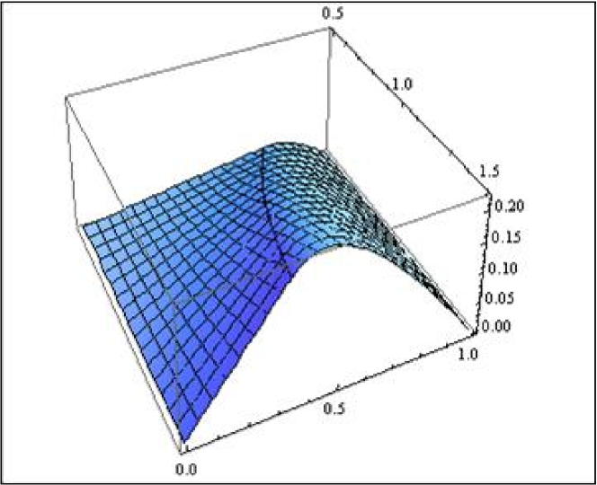
Figure 8: The value of the deformation parameter $\rho_{0}$ and the ground state energy $E_{0}$ as a function of $0\leq\chi\leq 1$ and $0.5\leq R^{2}\leq 1.5$.

6 Three-body clusters

The ACM for three identical clusters was introduced in hadron physics to describe the relative motion of three constituent quarks in a baryon [38], but more recently it has also found an interesting application in nuclear physics in which the properties of ¹²C are treated in terms of a cluster of three $\alpha$ particles [20, 32].

In this case, the building blocks of the model consist of two vector boson operators (one for each relative Jacobi coordinate) and a scalar boson

$$b^{\dagger}_{1,m}~{},\;b^{\dagger}_{2,m}~{},\;s^{\dagger}~{}.$$ (10lmnbedueh)

The set of 49 bilinear products of creation and annihilation operators spans the Lie algebra of $U(7)$. The model space contains the oscillator shells with $n=n_{1}+n_{2}=0,1,2,\ldots,N$. The ACM describes three-body cluster states in terms of a system of $N=n_{s}+n_{1}+n_{2}$ interacting bosons with angular momentum and parity $L^{P}=1^{-}$ (two vector bosons, $b_{1}^{\dagger}$ and $b_{2}^{\dagger}$) and $L^{P}=0^{+}$ (scalar boson, $s^{\dagger}$).

6.1 Geometrical symmetry

For three identical particles, such as $X_{3}$ molecules, $3\alpha$ clusters or $qqq$ baryons, the Hamiltonian has to be invariant under the permutation group $S_{3}$. All permutations of three objects can be expressed in terms of two elementary ones, the transposition $P(12)$ and the cyclic permutation $P(123)$. The transformation properties under $S_{3}$ of all operators in the model follow from those of the building block,

$$P(12)\left(\begin{array}[]{l}s^{\dagger}\\ b^{\dagger}_{1}\\ b^{\dagger}_{2}\end{array}\right) = U_{\rm tr}\left(\begin{array}[]{l}s^{\dagger}\\ b^{\dagger}_{1}\\ b^{\dagger}_{2}\end{array}\right)U^{-1}_{\rm tr}$$ (10lmnbedueo)

$$= \left(\begin{array}[]{rrr}1&0&0\\ 0&-1&0\\ 0&0&1\end{array}\right)\left(\begin{array}[]{l}s^{\dagger}\\ b^{\dagger}_{1}\\ b^{\dagger}_{2}\end{array}\right)~{},$$ (10lmnbeduev)

with

$$U_{\rm tr}=\mbox{e}^{i\pi b^{\dagger}_{1}b_{1}}~{},$$ (10lmnbeduew)

for the transposition $P(12)$, and

$$P(123)\left(\begin{array}[]{l}s^{\dagger}\\ b^{\dagger}_{1}\\ b^{\dagger}_{2}\end{array}\right) = U_{\rm cycl}\left(\begin{array}[]{l}s^{\dagger}\\ b^{\dagger}_{1}\\ b^{\dagger}_{2}\end{array}\right)U^{-1}_{\rm cycl}\hskip 56.9055pt$$ (10lmnbedufd)

$$= \left(\begin{array}[]{ccc}1&0&0\\ 0&-\frac{1}{2}&\frac{\sqrt{3}}{2}\\ 0&-\frac{\sqrt{3}}{2}&-\frac{1}{2}\end{array}\right)\left(\begin{array}[]{l}s^{\dagger}\\ b^{\dagger}_{1}\\ b^{\dagger}_{2}\end{array}\right)~{},$$ (10lmnbedufk)

with

$$U_{\rm cycl}=\mbox{e}^{i\pi(b^{\dagger}_{1}b_{1}+b^{\dagger}_{2}b_{2})}\,\mbox{e}^{\theta(b^{\dagger}_{1}b_{2}-b^{\dagger}_{2}b_{1})}~{},$$ (10lmnbedufl)

and $\theta=\arctan\sqrt{3}$ for the cyclic permutation $P(123)$. The scalar boson, $s^{\dagger}$, transforms as the symmetric representation $[3]$ of $S_{3}$, whereas the vector Jacobi bosons, $b^{\dagger}_{1}$ and $b^{\dagger}_{2}$, transform as the two components of the mixed symmetry representation.

There are three different symmetry classes for the permutation of three objects characterized by the Young tableaux

$$\begin{array}[]{ccccc}\begin{picture}(30.0,20.0)(0.0,0.0)\put(0.0,10.0){\line(1,0){30.0}} \put(0.0,0.0){\line(1,0){30.0}} \put(0.0,0.0){\line(0,1){10.0}} \put(10.0,0.0){\line(0,1){10.0}} \put(20.0,0.0){\line(0,1){10.0}} \put(30.0,0.0){\line(0,1){10.0}} \end{picture}&:&[3]&\sim&A_{1}\\ \begin{picture}(30.0,20.0)(0.0,0.0)\put(0.0,10.0){\line(1,0){20.0}} \put(0.0,0.0){\line(1,0){20.0}} \put(0.0,-10.0){\line(1,0){10.0}} \put(0.0,-10.0){\line(0,1){20.0}} \put(10.0,-10.0){\line(0,1){20.0}} \put(20.0,0.0){\line(0,1){10.0}} \end{picture}&:&[21]&\sim&E\\ \begin{picture}(30.0,30.0)(0.0,0.0)\put(0.0,10.0){\line(1,0){10.0}} \put(0.0,0.0){\line(1,0){10.0}} \put(0.0,-10.0){\line(1,0){10.0}} \put(0.0,-20.0){\line(1,0){10.0}} \put(0.0,-20.0){\line(0,1){30.0}} \put(10.0,-20.0){\line(0,1){30.0}} \end{picture}&:&[111]&\sim&A_{2}\\ &&&&\\ &&&&\end{array}$$ (10lmnbedufr)

The triangular configuration with three identical objects has point group symmetry ${\cal D}_{3h}$ [32]. Since ${\cal D}_{3h}\sim{\cal D}_{3}\times P$, the transformation properties under ${\cal D}_{3h}$ are labeled by parity $P$ and the representations of ${\cal D}_{3}\sim S_{3}$. Since $S_{3}$ is isomorphic to the point group ${\cal D}_{3}$, the irreducible representations can also be labeled by $[3]\sim A_{1}$ for the symmetric, $[111]\sim A_{2}$ for the antisymmetric, and $[21]\sim E$ for the mixed symmetry representations. Next, one can use the multiplication rules for $S_{3}$ (or ${\cal D}_{3}$) to construct physical operators with the appropriate symmetry properties. For example, for the bilinear products of the three vector Jacobi bosons, one finds

$$[21]\otimes[21]=[3]\oplus[21]\oplus[111]~{},$$ (10lmnbedufs)

or, equivalently,

$$E\otimes E=A_{1}\oplus E\oplus A_{2}~{}.$$ (10lmnbeduft)

$A_{1}$ and $A_{2}$ are one-dimensional representations, whereas $E$ is a two-fold degenerate representation.

6.2 Hamiltonian

For the case of three identical clusters, the Hamiltonian has to be invariant under the point group ${\cal D}_{3}\sim S_{3}$, and can be written as [38]

$$H = \epsilon_{0}\,s^{\dagger}\tilde{s}-\epsilon_{1}\,(b_{1}^{\dagger}\cdot\tilde{b}_{1}+b_{2}^{\dagger}\cdot\tilde{b}_{2})$$ (10lmnbedufu)

$$+u_{0}\,(s^{\dagger}s^{\dagger}\tilde{s}\tilde{s})-u_{1}\,s^{\dagger}(b_{1}^{\dagger}\cdot\tilde{b}_{1}+b_{2}^{\dagger}\cdot\tilde{b}_{2})\tilde{s}$$

$$+v_{0}\left[(b_{1}^{\dagger}\cdot b_{1}^{\dagger}+b_{2}^{\dagger}\cdot b_{2}^{\dagger})\tilde{s}\tilde{s}\right.$$

$$\hskip 28.45274pt\left.+s^{\dagger}s^{\dagger}(\tilde{b}_{1}\cdot\tilde{b}_{1}+\tilde{b}_{2}\cdot\tilde{b}_{2})\right]$$

$$+\sum_{L=0,2}a_{L}\,(b_{1}^{\dagger}b_{1}^{\dagger}+b_{2}^{\dagger}b_{2}^{\dagger})^{(L)}\cdot(\tilde{b}_{1}\tilde{b}_{1}+\tilde{b}_{2}\tilde{b}_{2})^{(L)}$$

$$+\sum_{L=0,2}b_{L}\left[(b_{1}^{\dagger}b_{1}^{\dagger}-b_{2}^{\dagger}b_{2}^{\dagger})^{(L)}\cdot\right.(\tilde{b}_{1}\tilde{b}_{1}-\tilde{b}_{2}\tilde{b}_{2})^{(L)}$$

$$\hskip 56.9055pt\left.+4\,(b_{1}^{\dagger}b_{2}^{\dagger})^{(L)}\cdot(\tilde{b}_{2}\tilde{b}_{1})^{(L)}\right]$$

$$+c_{1}\,(b_{1}^{\dagger}b_{2}^{\dagger})^{(1)}\cdot(\tilde{b}_{2}\tilde{b}_{1})^{(1)}~{}.$$

The first five terms are equivalent to those in Eq. (10lmnp), whereas the last three terms proportional to $a_{L}$, $b_{L}$ and $c_{1}$, correspond to interactions involving pairs of vector bosons with $A_{1}$, $E$ and $A_{2}$ symmetry, respectively (see Eq. (10lmnbeduft)). Since the cluster states arise entirely from the relative motion of the three clusters, and not from the internal excitations of the clusters, the allowed states have to be symmetric $t=A_{1}$. The discrete symmetry of the eigenfunctions can be determined from the matrix elements of $P(12)$ and $P(123)$ [38]. The invariance of $H$ under $P(12)$ allows one to distinguish between wave functions which are even and odd under $P(12)$

$$\left<\psi_{t}\right|P(12)\left|\psi_{t}\right>=\left<\psi_{t}\right|U_{\rm tr}\left|\psi_{t}\right>=\pm 1~{}.$$ (10lmnbedufv)

Algebraically, the matrix elements of the cyclic permutation can be written as

$$\left<\psi_{t}\right|P(123)\left|\psi_{t}\right>=\left<\psi_{t}\right|U_{\rm cycl}\left|\psi_{t}\right>~{}.$$ (10lmnbedufw)

The first term in $U_{\rm cycl}$ of Eq. (10lmnbedufl) gives rise to a phase factor $(-1)^{n_{1}+n_{2}}$ which is $+1$ ($-1$) for states with even (odd) parity. The second term corresponds to a transformation among oscillator coordinates, and therefore its matrix elements are given in terms of Talmi-Moshinksy brackets [53, 54] which were calculated with the program TMB [55]. In practice, the wave functions $\psi_{t}$ are obtained numerically by diagonalization, and hence are determined up to a sign. The relative phases of the degenerate representation $E$ with $E_{\rho}$ and $E_{\lambda}$, can be fixed by calculating the off-diagonal matrix elements of $P(123)$ and requiring that they transform like the components of the degenerate representations (see A). Summarizing, the symmetry character under ${\cal D}_{3}\sim S_{3}$ of any given wave function can be determined by comparing the matrix elements of $P(12)$ and $P(123)$ with the transformation properties listed in A.

6.3 Oblate top

A study of the classical limit of the $U(6)$ and $SO(7)$ dynamical symmetries of the Hamiltonian of Eq. (10lmnbedufu) shows that the corresponding potential energy surfaces only depend on the hyperspherical radius $\rho$ with equilibrium values $\rho_{0}=0$ and $\rho_{0}=1$, respectively (see Section 4). However, these are not the only possible equilibrium shapes. For example, consider the Hamiltonian [32, 38]

$$H_{\rm 3b} = \xi_{1}\,P^{\dagger}\tilde{P}+\xi_{2}\left[(b_{1}^{\dagger}\cdot b_{1}^{\dagger}-b_{2}^{\dagger}\cdot b_{2}^{\dagger})\,(\tilde{b}_{1}\cdot\tilde{b}_{1}-\tilde{b}_{2}\cdot\tilde{b}_{2})\right.$$ (10lmnbedufx)

$$\hskip 28.45274pt\left.+4\,(b_{1}^{\dagger}\cdot b_{2}^{\dagger})\,(\tilde{b}_{2}\cdot\tilde{b}_{1})\right]+\kappa\,\vec{L}\cdot\vec{L}~{},$$

where $P^{\dagger}$ is the generalized pairing operator

$$P^{\dagger}=R^{2}\,s^{\dagger}s^{\dagger}-b_{1}^{\dagger}\cdot b_{1}^{\dagger}-b_{2}^{\dagger}\cdot b_{2}^{\dagger}~{},$$ (10lmnbedufy)

and $\vec{L}$ the angular momentum

$$\hat{L}_{m}=\sqrt{2}\,(b^{\dagger}_{1}\tilde{b}_{1}+b^{\dagger}_{2}\tilde{b}_{2})^{(1)}_{m}~{}.$$ (10lmnbedufz)

For $R^{2}=1$ and $\xi_{2}=0$ the Hamiltonian has $U(7)\supset SO(7)$ symmetry and corresponds to a six-dimensional deformed oscillator. For $R^{2}=0$ there is no mixing between oscillator shells and the Hamiltonian is that of an anharmonic vibrator. In this section I will show that the general case with $R^{2}\neq 0$ and $\xi_{1}$, $\xi_{2}>0$ corresponds to an oblate symmetric top. Even though in this case the Hamiltonian does not have a dynamical symmetry, it is still possible to derive an approximate energy formula. The potential energy surface associated with the Hamiltonian of Eq. (10lmnbedufx) is obtained by taking the static limit of its classical limit, i.e. by setting all momenta equal to zero

$$V_{\rm cl}(\rho,\eta,\zeta)=\xi_{1}(N-1)\left[R^{2}-\frac{1}{2}\rho^{2}(1+R^{2})\right]^{2}$$

$$\hskip 28.45274pt+\xi_{2}(N-1)\frac{\rho^{4}}{4}\left(\cos^{2}2\eta+\sin^{2}2\eta\cos^{2}2\zeta\right)~{}.$$ (10lmnbeduga)

Its equilibrium configuration is characterized by coordinates that have equal length ($\rho_{1,0}=\rho_{2,0}=\rho_{0}/\sqrt{2}$) and are mutually perpendicular

$$\rho_{0} = \sqrt{2R^{2}/(1+R^{2})}~{},$$ (10lmnbedugba)

$$\eta_{0} = \pi/4~{},$$ (10lmnbedugbb)

$$\zeta_{0} = \pi/4~{},$$ (10lmnbedugbc)

where $2\zeta$ denotes the relative angle between $\vec{\alpha}_{1}$ and $\vec{\alpha}_{2}$. Geometrically, this equilibrium shape corresponds to three clusters located at the vertices of an equilateral triangle. In the limit of small oscillations around the minimum $\rho=\rho_{0}+\Delta\rho$, $\eta=\eta_{0}+\Delta\eta$ and $\zeta=\zeta_{0}+\Delta\zeta$, the intrinsic degrees of freedom $\rho$, $\eta$ and $\zeta$ decouple and become harmonic. To leading order in $N$ one finds

$$H_{\rm 3b,cl} = \xi_{1}N\left[\frac{2R^{2}}{1+R^{2}}p^{2}+2R^{2}(1+R^{2})(\Delta\rho)^{2}\right]$$ (10lmnbedugbgc)

$$+\xi_{2}N\left[p_{\eta}^{2}+\frac{4R^{4}}{(1+R^{2})^{2}}(\Delta\eta)^{2}\right.$$

$$\hskip 28.45274pt\left.+p_{\zeta}^{2}+\frac{4R^{4}}{(1+R^{2})^{2}}(\Delta\zeta)^{2}\right]~{}.$$

Standard quantization of the harmonic oscillator yields the vibrational energy spectrum of an oblate top

$$E_{\rm 3b,vib} = \omega_{1}(v_{1}+\frac{1}{2})+\omega_{2}(v_{2}+1)~{},$$ (10lmnbedugbgd)

with frequencies

$$\omega_{1} = 4NR^{2}\xi_{1}~{},$$ (10lmnbedugbgea)

$$\omega_{2} = \frac{4NR^{2}}{1+R^{2}}\xi_{2}~{},$$ (10lmnbedugbgeb)

in agreement with the results obtained in a normal mode analysis [38]. The vibrational part of the Hamiltonian of Eq. (10lmnbedufu) has a very simple physical interpretation in terms of the three fundamental vibrations of a triangular configuration (see Figure 9): $v_{1}$ represents the vibrational quantum number for a symmetric stretching $A$ vibration, and $v_{2}=v_{2a}+v_{2b}$ for a two-fold degenerate $E$ vibration. The rotational spectrum is given by

$$E_{\rm 3b,rot}=\kappa\,L(L+1)~{}.$$ (10lmnbedugbgegf)

Figure 9: Fundamental vibrations of a triangular configuration (point group ${\cal D}_{3h}$).

Fig. 10 shows the structure of the rotational excitations of the ground-state vibrational band $(v_{1}v_{2})=(00)$. For identical bosons, as is the case for a cluster of three $\alpha$-particles, the allowed states are symmetric with $t=A_{1}$, and therefore the rotational structure of the ground-state band is a sequence of states with angular momentum and parity $L^{P}=0^{+}$, $2^{+}$, $3^{-}$, $4^{\pm}$, $5^{-}$, $\ldots$, as shown in the right panel of Fig. 10.

Figure 10: Schematic spectrum of the rotational states of the ground stand vibrational band with $(v_{1}v_{2})=(00)$. The states are labeled by $L^{P}_{t}$. The right-hand panel shows the symmetric states with $t=A_{1}$.

Fig. 11 shows the rotation-vibration spectrum of the oblate top according to Eqs. (10lmnbedugbgd) and (10lmnbedugbgegf). The energy spectrum consists of a series of rotational bands labeled by $(v_{1},v_{2})$. The bands with $(v_{1},0)$ have angular momenta and parity $L^{P}=0^{+}$, $2^{+}$, $3^{-}$, $4^{\pm}$, $5^{-}$, $\ldots$, whereas the doubly degenerate vibrations with $(v_{1},1)$ have $L^{P}=1^{-}$, $2^{\mp}$, $3^{\mp}$, $\ldots$, in agreement with Ref. [56].

Figure 11: Schematic rotation-vibration spectrum of an oblate symmetric top. The rotational bands are labeled by $(v_{1}v_{2})$ (bottom), and the rotational excitations by $L^{P}$ (right). All states are symmetric under ${\cal D}_{3}\sim S_{3}$.

6.4 Electromagnetic couplings

For the case of three-body clusters, transition form factors and $B(EL)$ values are obtained from the matrix elements of the transition operator

$$\hat{T}(\epsilon) = e^{-iq\beta\hat{D}_{2,z}/X_{D}}~{},$$ (10lmnbedugbgegga)

$$\hat{D}_{2,m} = (b^{\dagger}_{2}\tilde{s}-s^{\dagger}\tilde{b}_{2})^{(1)}_{m}~{}.$$ (10lmnbedugbgeggb)

For the oblate top, the form factors can be obtained in closed form in the large $N$ limit. In this case, the normalization factor $X_{D}$ is given by

$$X_{D}=\frac{2NR}{(1+R^{2})\sqrt{2}}~{}.$$ (10lmnbedugbgegggh)

Just as for the case of two-body clusters, the transition form factors for transitions along the ground state band $(v_{1}v_{2})=(00)$ are given in terms of a spherical Bessel function $c_{L}j_{L}(q\beta)$, but now with

$$c_{L}^{2}=\frac{2L+1}{3}\left[1+2P_{L}(-\frac{1}{2})\right]~{}.$$ (10lmnbedugbgegggi)

The coefficient $c_{1}^{2}$ vanishes as a consequence of the triangular symmetry. Some values which are relevant to the lowest states are $c_{0}^{2}=1$, $c_{2}^{2}=5/4$, $c_{3}^{2}=35/8$, $c_{4}^{2}=81/64$ and $c_{5}^{2}=385/128$. For the extended charge distribution of Eq. (10lmnar) the form factors are multiplied by an exponential factor $\exp(-q^{2}/4\alpha)$.

The $B(EL;0\rightarrow L)$ values along the ground state band are given by the same formula as for the case of the axial rotor $(Zec_{L}\beta^{L})^{2}/4\pi$, the only difference being in the value of the coefficients $c_{L}^{2}$. In this case they are given by Eq. (10lmnbedugbgegggi). The resulting $B(EL)$ values are in agreement with the results of Eq. (9).

Form factors and $B(EL)$ values depend on $\alpha$, $\beta$ and $c_{L}$. The coefficients $\alpha$ and $\beta$ can be determined from the charge radius and the first minimum in the elastic form factor, whereas the $c_{L}$’s arise from the discrete symmetry of the triangular configuration of the three $\alpha$ particles. The analytic results given in this section provide a set of closed expressions which can be used to analyze and interpret the experimental data.

6.5 Shape-phase transition

The ACM describes the relative dynamics of a three-body system and contains both the harmonic oscillator, the deformed oscillator and the oblate top as special limits, as well as the region in between these limiting cases. The transitional region can be described by the schematic Hamiltonian

$$H = (1-\chi)\sum_{m}(b_{1,m}^{\dagger}b_{1,m}+b_{2,m}^{\dagger}b_{2,m})$$ (10lmnbedugbgegggj)

$$+\frac{\chi}{4(N-1)}\,P^{\dagger}\tilde{P}$$

$$+\frac{\xi}{N-1}\left[(b_{1}^{\dagger}\cdot b_{1}^{\dagger}-b_{2}^{\dagger}\cdot b_{2}^{\dagger})\,(\tilde{b}_{1}\cdot\tilde{b}_{1}-\tilde{b}_{2}\cdot\tilde{b}_{2})\right.$$

$$\hskip 56.9055pt\left.+4\,(b_{1}^{\dagger}\cdot b_{2}^{\dagger})\,(\tilde{b}_{2}\cdot\tilde{b}_{1})\right]~{},$$

with $0\leq\chi\leq 1$ and $\xi>0$. For $\chi=0$ it reduces to the harmonic oscillator with anharmonic terms proportional to $\xi$, and for $\chi=1$ to the oblate top of the previous section. For $\chi=1$, $R^{2}=1$ and $\xi=0$ it reduces to the deformed oscillator discussed in Section 4.2. The transitional region between any of these special cases can be studied in the classical limit of the Hamiltonian following the methods already discussed in Section 4.3. In this case, the potential energy surface is given by

$$V_{\rm cl}(\rho,\eta,\zeta) = \frac{1-\chi}{2}\,\rho^{2}+\frac{\chi}{4}\left[R^{2}-\frac{1}{2}\rho^{2}(1+R^{2})\right]^{2}$$ (10lmnbedugbgegggk)

$$+\frac{\xi\rho^{4}}{4}\left(\cos^{2}2\eta+\sin^{2}2\eta\cos^{2}2\zeta\right)~{}.$$

An analysis of the classical limit of the Hamiltonian of Eq. (10lmnbedugbgegggj) shows that $H$ exhibits a second-order phase transition between the spherical and deformed shapes. As before, the spherical shape is characterized by $\rho_{0}=0$, but in this case the deformed shape corresponds to three clusters located at the vertices of an equilateral triangle characterized by $\rho^{2}_{0}>0$, $\eta_{0}=\pi/4$ and $\zeta_{0}=\pi/4$. The value of the deformation parameter $\rho_{0}^{2}$ and the dependence of the critical point $\chi_{c}$ on $R^{2}$ are given by Eqs. (10lmnbeduef) and (10lmnbedueg), respectively.

7 Four-body clusters

The extension of the algebraic cluster model to four-body systems was introduced recently in an application to ¹⁶O as a cluster of four $\alpha$ particles [33, 40]. The ACM introduces a vector boson with $L^{P}=1^{-}$ for each independent relative Jacobi coordinate, together with a scalar boson with $L^{P}=0^{+}$

$$b^{\dagger}_{1,m}~{},\;b^{\dagger}_{2,m}~{},\;b^{\dagger}_{3,m}~{},\;s^{\dagger}~{}.$$ (10lmnbedugbgegggl)

This procedure leads to a compact spectrum generating algebra of $U(10)$ whose model space is spanned by the symmetric irreducible representation $[N]$ which contains the oscillator shells with $n=n_{1}+n_{2}+n_{3}=0,1,2,\ldots,N$.

7.1 Discrete symmetry

For four identical objects (e.g. for X₄ molecules and $4\alpha$ clusters) the Hamiltonian has to be invariant under the permuation group $S_{4}$. All permutations can be expressed in terms of the transposition $P(12)$ and the cyclic permutation $P(1234)$ [41]. The transformation properties under $S_{4}$ of all operators in the model follow from those of the building blocks,

$$P(12)\left(\begin{array}[]{l}s^{\dagger}\\ b^{\dagger}_{1}\\ b^{\dagger}_{2}\\ b^{\dagger}_{3}\end{array}\right)=U_{\rm tr}\left(\begin{array}[]{l}s^{\dagger}\\ b^{\dagger}_{1}\\ b^{\dagger}_{2}\\ b^{\dagger}_{3}\end{array}\right)U^{-1}_{\rm tr}$$ (10lmnbedugbgegggu)

$$\hskip 28.45274pt=\left(\begin{array}[]{rrrr}1&0&0&0\\ 0&-1&0&0\\ 0&0&1&0\\ 0&0&0&1\end{array}\right)\left(\begin{array}[]{l}s^{\dagger}\\ b^{\dagger}_{1}\\ b^{\dagger}_{2}\\ b^{\dagger}_{3}\end{array}\right)~{},$$ (10lmnbedugbgegghd)

with $U_{\rm tr}$ defined in Eq. (10lmnbeduew) for the transposition $P(12)$, and

$$P(1234)\left(\begin{array}[]{l}s^{\dagger}\\ b^{\dagger}_{1}\\ b^{\dagger}_{2}\\ b^{\dagger}_{3}\end{array}\right)=U_{\rm cycl}\left(\begin{array}[]{l}s^{\dagger}\\ b^{\dagger}_{1}\\ b^{\dagger}_{2}\\ b^{\dagger}_{3}\end{array}\right)U^{-1}_{\rm cycl}$$ (10lmnbedugbgegghm)

$$\hskip 28.45274pt=\left(\begin{array}[]{cccc}1&0&0&0\\ 0&-\frac{1}{2}&\frac{\sqrt{3}}{2}&0\\ 0&-\frac{1}{2\sqrt{3}}&-\frac{1}{6}&\frac{\sqrt{8}}{3}\\ 0&-\frac{\sqrt{2}}{\sqrt{3}}&-\frac{\sqrt{2}}{3}&-\frac{1}{3}\end{array}\right)\left(\begin{array}[]{l}s^{\dagger}\\ b^{\dagger}_{1}\\ b^{\dagger}_{2}\\ b^{\dagger}_{3}\end{array}\right)~{},$$ (10lmnbedugbgegghv)

with

$$U_{\rm cycl} = \mbox{e}^{i\pi(b^{\dagger}_{1}b_{1}+b^{\dagger}_{2}b_{2}+b^{\dagger}_{3}b_{3})}\,\mbox{e}^{\theta_{1}(b^{\dagger}_{1}b_{2}-b^{\dagger}_{2}b_{1})}\,\mbox{e}^{\theta_{2}(b^{\dagger}_{2}b_{3}-b^{\dagger}_{3}b_{2})}~{},$$

and $\theta_{1}=\arctan\sqrt{3}$ and $\theta_{2}=\arctan\sqrt{8}$, for the cyclic permutation $P(1234)$. The scalar boson, $s^{\dagger}$, transforms as the symmetric representation $[4]$ of $S_{4}$, whereas the three vector Jacobi bosons, $b^{\dagger}_{1}$, $b^{\dagger}_{2}$ and $b^{\dagger}_{3}$, transform as the three components of the mixed symmetry representation $[31]$.

There are five different symmetry classes for the permutation of four objects characterized by the Young tableaux

$$\begin{array}[]{ccccc}\begin{picture}(40.0,20.0)(0.0,0.0)\put(0.0,10.0){\line(1,0){40.0}} \put(0.0,0.0){\line(1,0){40.0}} \put(0.0,0.0){\line(0,1){10.0}} \put(10.0,0.0){\line(0,1){10.0}} \put(20.0,0.0){\line(0,1){10.0}} \put(30.0,0.0){\line(0,1){10.0}} \put(40.0,0.0){\line(0,1){10.0}} \end{picture}&:&[4]&\sim&A_{1}\\ \begin{picture}(40.0,20.0)(0.0,0.0)\put(0.0,10.0){\line(1,0){30.0}} \put(0.0,0.0){\line(1,0){30.0}} \put(0.0,-10.0){\line(1,0){10.0}} \put(0.0,-10.0){\line(0,1){20.0}} \put(10.0,-10.0){\line(0,1){20.0}} \put(20.0,0.0){\line(0,1){10.0}} \put(30.0,0.0){\line(0,1){10.0}} \end{picture}&:&[31]&\sim&F_{2}\\ &&&&\\ \begin{picture}(40.0,20.0)(0.0,0.0)\put(0.0,10.0){\line(1,0){20.0}} \put(0.0,0.0){\line(1,0){20.0}} \put(0.0,-10.0){\line(1,0){20.0}} \put(0.0,-10.0){\line(0,1){20.0}} \put(10.0,-10.0){\line(0,1){20.0}} \put(20.0,-10.0){\line(0,1){20.0}} \end{picture}&:&[22]&\sim&E\\ \begin{picture}(40.0,30.0)(0.0,0.0)\put(0.0,10.0){\line(1,0){20.0}} \put(0.0,0.0){\line(1,0){20.0}} \put(0.0,-10.0){\line(1,0){10.0}} \put(0.0,-20.0){\line(1,0){10.0}} \put(0.0,-20.0){\line(0,1){30.0}} \put(10.0,-20.0){\line(0,1){30.0}} \put(20.0,0.0){\line(0,1){10.0}} \end{picture}&:&[211]&\sim&F_{1}\\ \begin{picture}(40.0,40.0)(0.0,0.0)\put(0.0,10.0){\line(1,0){10.0}} \put(0.0,0.0){\line(1,0){10.0}} \put(0.0,-10.0){\line(1,0){10.0}} \put(0.0,-20.0){\line(1,0){10.0}} \put(0.0,-30.0){\line(1,0){10.0}} \put(0.0,-30.0){\line(0,1){40.0}} \put(10.0,-30.0){\line(0,1){40.0}} \end{picture}&:&[1111]&\sim&A_{2}\\ &&&&\\ &&&&\\ &&&&\end{array}$$ (10lmnbedugbgeggig)

Since $S_{4}$ is isomorphic to the tetrahedral group ${\cal T}_{d}$, the irreducible representations can also be labeled by $[4]\sim A_{1}$ for the symmetric, $[1111]\sim A_{2}$ for the antisymmetric, and $[31]\sim F_{2}$, $[22]\sim E$ and $[211]\sim F_{1}$ for the mixed symmetry representations. Next, one can use the multiplication rules for $S_{4}$ (or ${\cal T}_{d}$) to construct physical operators with the appropriate symmetry properties. For example, for the bilinear products of the three vector Jacobi bosons, one finds

$$[31]\otimes[31]=[4]\oplus[31]\oplus[211]\oplus[22]~{},$$ (10lmnbedugbgeggih)

or, equivalently,

$$F_{2}\otimes F_{2}=A_{1}\oplus F_{2}\oplus F_{1}\oplus E~{}.$$ (10lmnbedugbgeggii)

7.2 Hamiltonian

The ACM Hamiltonian that describes the relative motion of a system of four identical clusters has to be invariant under the tetrahedral group ${\cal T}_{d}\sim S_{4}$, and can be written as

$$H = \epsilon_{0}\,s^{\dagger}\tilde{s}-\epsilon_{1}\,(b_{1}^{\dagger}\cdot\tilde{b}_{1}+b_{2}^{\dagger}\cdot\tilde{b}_{2}+b_{3}^{\dagger}\cdot\tilde{b}_{3})$$ (10lmnbedugbgeggij)

$$+u_{0}\,s^{\dagger}s^{\dagger}\tilde{s}\tilde{s}$$

$$-u_{1}\,s^{\dagger}(b_{1}^{\dagger}\cdot\tilde{b}_{1}+b_{2}^{\dagger}\cdot\tilde{b}_{2}+b_{3}^{\dagger}\cdot\tilde{b}_{3})\tilde{s}$$

$$+v_{0}\left[(b_{1}^{\dagger}\cdot b_{1}^{\dagger}+b_{2}^{\dagger}\cdot b_{2}^{\dagger}+b_{3}^{\dagger}\cdot b_{3}^{\dagger})\tilde{s}\tilde{s}+{\rm h.c.}\right]$$

$$+\sum_{L=0,2}a_{L}\,(b_{1}^{\dagger}b_{1}^{\dagger}+b_{2}^{\dagger}b_{2}^{\dagger}+b_{3}^{\dagger}b_{3}^{\dagger})^{(L)}\cdot({\rm h.c.})$$

$$+\sum_{L=0,2}b_{L}\left[(-2\sqrt{2}\,b_{1}^{\dagger}b_{3}^{\dagger}+2b_{1}^{\dagger}b_{2}^{\dagger})^{(L)}\cdot({\rm h.c.})\right.$$

$$\hskip 7.11317pt+\left.(-2\sqrt{2}\,b_{2}^{\dagger}b_{3}^{\dagger}+b_{1}^{\dagger}b_{1}^{\dagger}-b_{2}^{\dagger}b_{2}^{\dagger})^{(L)}\cdot({\rm h.c.})\right]$$

$$+\sum_{L=0,2}c_{L}\left[(2b_{1}^{\dagger}b_{3}^{\dagger}+2\sqrt{2}\,b_{1}^{\dagger}b_{2}^{\dagger})^{(L)}\cdot({\rm h.c.})\right.$$

$$\hskip 7.11317pt+(2b_{2}^{\dagger}b_{3}^{\dagger}+\sqrt{2}(b_{1}^{\dagger}b_{1}^{\dagger}-b_{2}^{\dagger}b_{2}^{\dagger}))^{(L)}\cdot({\rm h.c.})$$

$$\hskip 7.11317pt\left.+(b_{1}^{\dagger}b_{1}^{\dagger}+b_{2}^{\dagger}b_{2}^{\dagger}-2b_{3}^{\dagger}b_{3}^{\dagger})^{(L)}\cdot({\rm h.c.})\right]$$

$$+c_{1}\left[(b_{1}^{\dagger}b_{2}^{\dagger})^{(1)}\cdot(\tilde{b}_{2}\tilde{b}_{1})^{(1)}\right.+(b_{2}^{\dagger}b_{3}^{\dagger})^{(1)}\cdot(\tilde{b}_{3}\tilde{b}_{2})^{(1)}$$

$$\hskip 28.45274pt\left.+(b_{3}^{\dagger}b_{1}^{\dagger})^{(1)}\cdot(\tilde{b}_{1}\tilde{b}_{3})^{(1)}\right]~{}.$$

The first five terms are equivalent to those in Eq. (10lmnp), whereas the last four terms proportional to $a_{L}$, $b_{L}$, $c_{L}$ and $c_{1}$, according to the product of Eq. (10lmnbedugbgeggii), correspond to interactions involving pairs of vector bosons with $A_{1}$, $E$, $F_{2}$ and $F_{1}$ symmetry, respectively.

In general, the eigenvalues and corresponding eigenvectors are obtained numerically. The wave functions are characterized by the quantum numbers $N$, $L^{P}_{t}$, where $N=n_{s}+n_{1}+n_{2}+n_{3}$ is the total number of bosons, $L$ the angular momentum, $P$ the parity, and $t$ the transformation property $t$ under the tetrahedral group ${\cal T}_{d}$. Since internal excitations of the clusters are not considered, the four-body wave functions arise solely from the relative motion and have to be symmetric ($t=A_{1}$).

The discrete symmetry $t$ of a given wave function can be determined as follows. Since the invariance of the Hamiltonian of Eq. (10lmnbedugbgeggij) under the transposition $P(12)$ implies that basis states with $n_{1}$ even and $n_{1}$ odd do not mix, wave functions which are even and odd under $P(12)$ can be distinguished by

$$\left<\psi_{t}\right|P(12)\left|\psi_{t}\right>=\left<\psi_{t}\right|U_{\rm tr}\left|\psi_{t}\right>=\pm 1~{}.$$ (10lmnbedugbgeggik)

The expectation value of the cyclic permutation $P(1234)$ can be obtained from

$$\left<\psi_{t}\right|P(1234)\left|\psi_{t}\right>=\left<\psi_{t}\right|U_{\rm cycl}\left|\psi_{t}\right>~{}.$$ (10lmnbedugbgeggil)

The first term in $U_{\rm cycl}$ of Eq. (LABEL:p1234) gives rise to a phase factor $(-1)^{n_{1}+n_{2}+n_{3}}$ which is $+1$ ($-1$) for states with even (odd) parity. The second and third terms in $U_{\rm cycl}$ can be expressed in terms of Talmi-Moshinksy brackets [53, 54]. The permutation symmetry of any given wave function is then determined from the matrix elements of $P(12)$ and $P1234)$ (see B). In practice, the wave functions $\psi_{t}$ are obtained numerically by diagonalization, and hence are determined up to a sign. The relative phases of the degenerate representations (the two-dimensional $E$ with $E_{\rho}$ and $E_{\lambda}$, and the three-dimensional $F_{2}$ with $F_{2\rho}$, $F_{2\lambda}$ and $F_{2\eta}$, and $F_{1}$ with $F_{1\rho}$, $F_{1\lambda}$ and $F_{1\eta}$) can be determined from the off-diagonal matrix elements of $P(1234)$ requiring that they transform as the components of the degenerate representations (see B).

7.3 Spherical top

In a study of the classical limit of the $U(9)$ and $SO(10)$ dynamical symmetries of Eq. (10lmnbedugbgeggij) presented in Section 4 it was shown that the corresponding potential energy surfaces only depend on the hyperspherical radius $\rho$. In general, the potential energy surface of the Hamiltonian of Eq. (10lmnbedugbgeggij) depends on the three Jacobi coordinates, $\rho$, $\eta_{1}$ and $\eta_{2}$ in the hypersperical notation of Eq. (10lmnbea-10lmnbec), and the three relative angles between the Jacobi vectors, $\zeta_{12}$, $\zeta_{23}$ and $\zeta_{31}$, In this section, I analyze the properties of the Hamiltonian introduced in [33] in a study of the $4\alpha$-cluster states of the nucleus ¹⁶O

$$H_{4b} = \xi_{1}\,P^{\dagger}\tilde{P}$$ (10lmnbedugbgeggim)

$$+\xi_{2}\left[(-2\sqrt{2}\,b_{1}^{\dagger}\cdot b_{3}^{\dagger}+2b_{1}^{\dagger}\cdot b_{2}^{\dagger})\,({\rm h.c.})\right.$$

$$\hskip 7.11317pt+\left.(-2\sqrt{2}\,b_{2}^{\dagger}\cdot b_{3}^{\dagger}+b_{1}^{\dagger}\cdot b_{1}^{\dagger}-b_{2}^{\dagger}\cdot b_{2}^{\dagger})\,({\rm h.c.})\right]$$

$$+\xi_{3}\left[(2b_{1}^{\dagger}\cdot b_{3}^{\dagger}+2\sqrt{2}\,b_{1}^{\dagger}\cdot b_{2}^{\dagger})\,({\rm h.c.})\right.$$

$$\hskip 7.11317pt+(2b_{2}^{\dagger}\cdot b_{3}^{\dagger}+\sqrt{2}\,(b_{1}^{\dagger}\cdot b^{\dagger}_{1}-b_{2}^{\dagger}\cdot b_{2}^{\dagger}))\,({\rm h.c.})$$

$$\hskip 7.11317pt\left.+(b_{1}^{\dagger}\cdot b_{1}^{\dagger}+b_{2}^{\dagger}\cdot b_{2}^{\dagger}-2b_{3}^{\dagger}\cdot b_{3}^{\dagger})\,({\rm h.c.})\right]$$

$$+\kappa_{1}\,\vec{L}\cdot\vec{L}+\kappa_{2}\,(\vec{L}\cdot\vec{L}-\vec{I}\cdot\vec{I})^{2}~{},$$

where $P^{\dagger}$ is the generalized pairing operator

$$P^{\dagger}=R^{2}\,s^{\dagger}s^{\dagger}-b_{1}^{\dagger}\cdot b_{1}^{\dagger}-b_{2}^{\dagger}\cdot b_{2}^{\dagger}-b_{3}^{\dagger}\cdot b_{3}^{\dagger}~{},$$ (10lmnbedugbgeggin)

$\vec{L}$ denotes the angular momentum in coordinate space

$$\hat{L}_{m}=\sqrt{2}\,(b^{\dagger}_{1}\tilde{b}_{1}+b^{\dagger}_{2}\tilde{b}_{2}+b^{\dagger}_{3}\tilde{b}_{3})^{(1)}_{m}~{},$$ (10lmnbedugbgeggio)

and $\vec{I}$ the angular momentum in index space

$$\hat{I}_{1} = -i\sum_{m}\left(b^{\dagger}_{2,m}b_{3,m}-b^{\dagger}_{3,m}b_{2,m}\right)~{},$$ (10lmnbedugbgeggipa)

$$\hat{I}_{2} = -i\sum_{m}\left(b^{\dagger}_{3,m}b_{1,m}-b^{\dagger}_{1,m}b_{3,m}\right)~{},$$ (10lmnbedugbgeggipb)

$$\hat{I}_{3} = -i\sum_{m}\left(b^{\dagger}_{1,m}b_{2,m}-b^{\dagger}_{2,m}b_{1,m}\right)~{}.$$ (10lmnbedugbgeggipc)

For $R^{2}=1$ and $\xi_{2}=\xi_{3}=0$ the Hamiltonian has $U(10)\supset SO(10)$ symmetry and corresponds to a nine-dimensional deformed oscillator. For $R^{2}=0$ there is no mixing between oscillator shells and the Hamiltonian is that of an anharmonic vibrator. In this section I discuss the general case with $R^{2}\neq 0$ and $\xi_{1}$, $\xi_{2}$, $\xi_{3}>0$, The potential energy surface associated with the Hamiltonian of Eq. (10lmnbedugbgeggim) has an equilibrium configuration corresponding to coordinates that have equal length ($\rho_{1,0}=\rho_{2,0}=\rho_{3,0}=\rho_{0}/\sqrt{3}$)

$$\rho_{0} = \sqrt{2R^{2}/(1+R^{2})}~{},$$ (10lmnbedugbgeggipiqa)

$$\eta_{1,0} = \arctan\sqrt{2}~{},$$ (10lmnbedugbgeggipiqb)

$$\eta_{2,0} = \pi/4~{},$$ (10lmnbedugbgeggipiqc)

and are mutually perpendicular

$$\zeta_{12,0}=\zeta_{23,0}=\zeta_{31,0}=\pi/4~{},$$ (10lmnbedugbgeggipiqd)

where $2\zeta_{ij}$ denotes the relative angle between $\vec{\alpha}_{i}$ and $\vec{\alpha}_{j}$. Just as in the case of the oblate top, the intrinsic degrees of freedom decouple in the limit of small oscillations around the equilibrium shape $\rho=\rho_{0}+\Delta\rho$, $\eta_{i}=\eta_{i,0}+\Delta\eta_{i}$ and $\zeta_{ij}=\zeta_{ij,0}+\Delta\zeta_{ij}$, and become harmonic. To leading order in $N$ one obtains

$$H_{\rm 4b,cl} = \xi_{1}N\left[\frac{2R^{2}}{1+R^{2}}p^{2}+2R^{2}(1+R^{2})(\Delta\rho)^{2}\right]$$ (10lmnbedugbgeggipiqir)

$$+\xi_{2}N\left[9p_{\nu_{2a}}^{2}+\frac{16R^{4}}{9(1+R^{2})^{2}}(\Delta\nu_{2a})^{2}\right.$$

$$\hskip 28.45274pt\left.+9p_{\nu_{2b}}^{2}+\frac{16R^{4}}{9(1+R^{2})^{2}}(\Delta\nu_{2b})^{2}\right]$$

$$+\xi_{3}N\left[9p_{\nu_{3a}}^{2}+\frac{16R^{4}}{9(1+R^{2})^{2}}(\Delta\nu_{3a})^{2}\right.$$

$$\hskip 28.45274pt+9p_{\nu_{3b}}^{2}+\frac{16R^{4}}{9(1+R^{2})^{2}}(\Delta\nu_{3b})^{2}$$

$$\hskip 28.45274pt\left.2p_{\eta_{1}}^{2}+\frac{8R^{4}}{(1+R^{2})^{2}}(\Delta\eta_{1})^{2}\right]~{},$$

where the $\Delta\nu$’s denote the oscillations

$$\Delta\nu_{2a} = \Delta\zeta_{12}-\sqrt{2}\,\Delta\zeta_{31}~{},$$ (10lmnbedugbgeggipiqisa)

$$\Delta\nu_{2b} = \Delta\eta_{2}-\sqrt{2}\,\Delta\zeta_{23}~{},$$ (10lmnbedugbgeggipiqisb)

$$\Delta\nu_{3a} = \Delta\zeta_{31}+\sqrt{2}\,\Delta\zeta_{12}~{},$$ (10lmnbedugbgeggipiqisc)

$$\Delta\nu_{3b} = \Delta\zeta_{23}+\sqrt{2}\,\Delta\eta_{2}~{},$$ (10lmnbedugbgeggipiqisd)

and the $p_{\nu}$’s the canonically conjugate momenta. Standard quantization gives the vibrational energy spectrum of a spherical top with tetrahedral symmetry

$$E_{\rm 4b,vib}=\omega_{1}(v_{1}+\frac{1}{2})+\omega_{2}(v_{2}+1)+\omega_{3}(v_{3}+\frac{3}{2})$$ (10lmnbedugbgeggipiqisit)

with frequencies

$$\omega_{1} = 4NR^{2}\xi_{1}~{},$$ (10lmnbedugbgeggipiqisiua)

$$\omega_{2} = \frac{8NR^{2}}{1+R^{2}}\xi_{2}~{},$$ (10lmnbedugbgeggipiqisiub)

$$\omega_{3} = \frac{8NR^{2}}{1+R^{2}}\xi_{3}~{},$$ (10lmnbedugbgeggipiqisiuc)

in agreement with the results obtained in a normal mode analysis of a spherical top with tetrahedral symmetry (see Fig. 12). Here $v_{1}$ represents the vibrational quantum number for a symmetric stretching vibration with $A_{1}$ symmetry, $v_{2}=v_{2a}+v_{2b}$ denotes a doubly degenerate vibration with $E$ symmetry, and $v_{3}=v_{3a}+v_{3b}+v_{3c}$ a three-fold degenerate vibration with $F_{2}$ symmetry. For rigid configurations, $R^{2}=1$ and $\omega_{i}=4N\xi_{i}$ with $i=1,2,3$.

Figure 12: Fundamental vibrations of a tetrahedral configuration (point group ${\cal T}_{d}$).

Note, that in general the angular momentum in index space $I$ is not conserved by ${\cal T}_{d}\sim S_{4}$ invariant interactions. Only if $a_{L}=c_{L}$ in Eq. (10lmnbedugbgeggij) or $\xi_{2}=\xi_{3}$ in Eq. (10lmnbedugbgeggim), does $I$ become a good quantum number for all eigenstates. Nevertheless, the general Hamiltonian of Eq. (10lmnbedugbgeggim) still has some eigenstates with good $I$: the rotational excitations of the ground state band with $(v_{1}v_{2}v_{3})=(000)$ are characterized by $I=L$. This can be understood from the fact that the operator $\vec{L}\cdot\vec{L}-\vec{I}\cdot\vec{I}$ annihilates the coherent (or intrinisic) state corresponding to the equilibrium shape of a regular tetrahedron, see Eqs. (10lmnbedugbgeggipiqa-10lmnbedugbgeggipiqd). As a consequence, the rotational energies of the ground state band are given by

$$E_{\rm 4b,rot}=\kappa_{1}L(L+1)~{}.$$ (10lmnbedugbgeggipiqisiuiv)

Figure 13: Schematic spectrum of the rotational states of the ground stand vibrational band with $(v_{1}v_{2}v_{3})=(000)$. All states have $L=I$ and are labeled by $L^{P}_{t}$. The right-hand panel shows the symmetric states with $t=A_{1}$.

Fig. 13 shows the structure of the rotational states of the ground state band $(v_{1}v_{2}v_{3})=(000)$. The rotational levels are doubled because of inversion doubling: for each value of the angular momentum $L$, one has doublets of states with ($A_{1}$, $A_{2}$), ($E$, $E$) and ($F_{2}$, $F_{1}$), in agreement with the classification of rotational levels of a spherical top with tetrahedral symmetry [56].

For identical bosons, as is the case for a cluster of four $\alpha$-particles, the allowed rotational-vibrational states are symmetric with $t=A_{1}$, and therefore the states of the ground state band $(v_{1}v_{2}v_{3})=(000)$ have angular momentum and parity $L^{P}=0^{+}$, $3^{-}$, $4^{+}$, $6^{\pm}$, $\ldots$, as shown in the right panel of Fig. 13. A similar analysis can be done for the rotational bands built on the $(100)A_{1}$, $(010)E$ and $(001)F_{2}$ vibrations. For the $A_{1}$ vibration the values of angular momentum and parity are the same as for the ground state band $L^{P}=0^{+}$, $3^{-}$, $4^{+}$, $6^{\pm}$, $\ldots$. For the double degenerate $E$ vibration they are $L^{P}=2^{\pm}$, $4^{\pm}$, $5^{\pm}$, $6^{\pm}$, $\ldots$, while for the triple degenerate $F_{2}$ vibration they are $L^{P}=1^{-}$, $2^{+}$, $3^{\pm}$, $4^{\pm}$, $5^{-,\pm}$, $6^{+,\pm}$ $\ldots$. The situation is summarized in Fig. 14 which shows the expected spectrum of a spherical top with tetrahedral symmetry and $\omega_{1}=\omega_{2}=\omega_{3}$.

Figure 14: Schematic rotation-vibration spectrum of a spherical top with tetrahedral symmetry and $\omega_{1}=\omega_{2}=\omega_{3}$. The rotational bands are labeled by $(v_{1}v_{2}v_{3})$ (bottom). All states are symmetric under $S_{4}\sim{\cal T}_{d}$.

7.4 Electromagnetic couplings

For four-body clusters, electromagnetic couplings can be obtained from the matrix elements of the transition operator

$$\hat{T}(\epsilon) = e^{-iq\beta\hat{D}_{3,z}/X_{D}}~{},$$ (10lmnbedugbgeggipiqisiuiwa)

$$\hat{D}_{3,m} = (b^{\dagger}_{3}\tilde{s}-s^{\dagger}\tilde{b}_{3})^{(1)}_{m}~{}.$$ (10lmnbedugbgeggipiqisiuiwb)

For the spherical top, the form factors can be obtained in closed form in the large $N$ limit. The normalization factor $X_{D}$ is given by

$$X_{D}=\frac{2NR}{(1+R^{2})\sqrt{3}}~{}.$$ (10lmnbedugbgeggipiqisiuiwix)

Also in this case, the transition form factors for transitions along the ground state band $(v_{1}v_{2}v_{3})=(000)$ are given in terms of a spherical Bessel function $c_{L}j_{L}(q\beta)$, but with

$$c_{L}^{2}=\frac{2L+1}{4}\left[1+3P_{L}(-\frac{1}{3})\right]~{}.$$ (10lmnbedugbgeggipiqisiuiwiy)

The coefficients $c_{1}^{2}$, $c_{2}^{2}$ and $c_{5}^{2}$ vanish as a consequence of the tetrahedral symmetry, Some values which are relevant to the lowest states are $c_{0}^{2}=1$, $c_{3}^{2}=35/9$, $c_{4}^{2}=7/3$ and $c_{6}^{2}=416/81$. For the extended charge distribution of Eq. (10lmnar) the form factors are multiplied by an exponential factor $\exp(-q^{2}/4\alpha)$.

Just as for the oblate top, the transition probabilities $B(EL;0\rightarrow L)$ along the ground state band are given by the same formula as for the case of the axial rotor $(Zec_{L}\beta^{L})^{2}/4\pi$, but with the coefficients $c_{L}^{2}$ from Eq. (10lmnbedugbgeggipiqisiuiwiy). The $B(EL)$ values are in agreement with the results of Eq. (10k).

Form factors and $B(EL)$ values depend on the coefficients $\alpha$, $\beta$, and $c_{L}$. Just as for two- and three-body clusters, the coefficients $\alpha$ and $\beta$ can be determined from the charge radius and the first minimum in the elastic form factor. The $c_{L}$’s are the consequence of the tetrahedral symmetry of the geometrical configuration of the four $\alpha$ particles.

7.5 Shape-phase transition

The ACM for four-body systems contains the harmonic oscillator, the deformed oscillator and the spherical top as special limits, as well as the region in between these limiting cases. The transitional region can be described by the schematic Hamiltonian

$$H = (1-\chi)\sum_{m}(b_{1,m}^{\dagger}b_{1,m}+b_{2,m}^{\dagger}b_{2,m}+b_{3,m}^{\dagger}b_{3,m})$$ (10lmnbedugbgeggipiqisiuiwiz)

$$+\frac{\chi}{4(N-1)}\,P^{\dagger}\tilde{P}$$

$$+\frac{\xi^{\prime}_{2}}{N-1}\left[(-2\sqrt{2}\,b_{1}^{\dagger}\cdot b_{3}^{\dagger}+2b_{1}^{\dagger}\cdot b_{2}^{\dagger})\,({\rm h.c.})\right.$$

$$\hskip 7.11317pt+\left.(-2\sqrt{2}\,b_{2}^{\dagger}\cdot b_{3}^{\dagger}+b_{1}^{\dagger}\cdot b_{1}^{\dagger}-b_{2}^{\dagger}\cdot b_{2}^{\dagger})\,({\rm h.c.})\right]$$

$$+\frac{\xi^{\prime}_{3}}{N-1}\left[(2b_{1}^{\dagger}\cdot b_{3}^{\dagger}+2\sqrt{2}\,b_{1}^{\dagger}\cdot b_{2}^{\dagger})\,({\rm h.c.})\right.$$

$$\hskip 7.11317pt+(2b_{2}^{\dagger}\cdot b_{3}^{\dagger}+\sqrt{2}\,(b_{1}^{\dagger}\cdot b^{\dagger}_{1}-b_{2}^{\dagger}\cdot b_{2}^{\dagger}))\,({\rm h.c.})$$

$$\hskip 7.11317pt\left.+(b_{1}^{\dagger}\cdot b_{1}^{\dagger}+b_{2}^{\dagger}\cdot b_{2}^{\dagger}-2b_{3}^{\dagger}\cdot b_{3}^{\dagger})\,({\rm h.c.})\right]~{},$$

with $0\leq\chi\leq 1$, $\xi^{\prime}_{2}>0$ and $\xi^{\prime}_{3}>0$. For $\chi=0$ it reduces to the harmonic oscillator with anharmonic terms proportional to $\xi^{\prime}_{2}$ and $\xi^{\prime}_{3}$, and for $\chi=1$ to the spherical top of the previous section. For $\chi=1$, $R^{2}=1$ and $\xi^{\prime}_{2}=\xi^{\prime}_{3}=0$ it reduces to the deformed oscillator discussed in Section 4.2. The transitional region can be studied by analyzing the properties of the corresponding potential energy surface. The terms proportional to $\xi^{\prime}_{2}$ and $\xi^{\prime}_{3}$ (both $>0$) favor an equilibrium shape in which the coordinates have equal length and are mutually perpendicular, see Eqs.(10lmnbedugbgeggipiqa-10lmnbedugbgeggipiqd). In addition, the equilibrium configuration is characterized by $\rho_{0}$ which changes from spherical $\rho_{0}=0$ to deformed $\rho_{0}^{2}>0$ as a function of $\chi$ according to Eq. (10lmnbeduef).

An analysis of the classical limit of the Hamiltonian of Eq. (10lmnbedugbgeggipiqisiuiwiz) shows that $H$ exhibits a second-order phase transition between the spherical and deformed shapes. As in the previous examples for two- and three-body clusters, the critical point depends on $R^{2}$ and is given by Eq. (10lmnbedueg). The dependence of the equilibrium shape and the ground state energy on $\chi$ and $R^{2}$ is the same as for the two-body ACM shown in Fig. 8. In this case, the equilibrium shape in the deformed region corresponds to four clusters located at the vertices of a regular tetrahedron.

8 Applications to $\alpha$-cluster nuclei

Evidence for $\alpha$ clustering in light nuclei can be found in a plot of the binding energy per nucleon which shows maxima for nuclei with $A=4k$, i.e. for the nuclei ⁴He, ⁸Be, ¹²C and ¹⁶O for $k=1$, 2, 3 and 4, respectively. In this secion, it is shown that further evidence can be found in the spectroscopy of $\alpha$-cluster states in ¹²C [20, 32] and ¹⁶O [33]. It is discussed how the structure of rotational bands can be used to obtain information about the underlying geometric configuration of the $\alpha$-clusters, and hence to distinguish between different theoretical approaches of $\alpha$-cluster nuclei.

8.1 The nucleus ¹²C

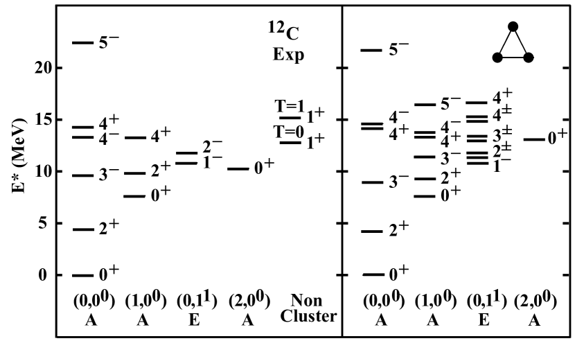
Figure 15: Comparison between the low-lying experimental spectrum of ¹²C and the energies of the oblate symmetric top calculated using Eq. (10lmnbedugbgeggipiqisiuiwja). The last column on the left-hand side, shows the lowest observed non-cluster levels with $J^{P}=1^{+}$ and $T=0$, $1$.

.

Fig. 15 shows a comparison of the cluster states of ¹²C with the spectrum of the oblate top according to the approximate energy formula [20]

$$E = E_{0}+\omega_{1}(v_{1}+\frac{1}{2})\left(1-\frac{v_{1}+\frac{1}{2}}{N}\right)$$ (10lmnbedugbgeggipiqisiuiwja)

$$+\omega_{2}(v_{2}+1)\left(1-\frac{v_{2}+1}{N+\frac{1}{2}}\right)$$

$$+\kappa_{1}L(L+1)+\kappa_{2}(K\mp 2\ell_{2})^{2}$$

$$+\left[\lambda_{1}(v_{1}+\frac{1}{2})+\lambda_{2}(v_{2}+1)\right]L(L+1)~{}.$$

The coefficients $\kappa_{1}$, $\lambda_{1}$ and $\lambda_{2}$ determine the moments of inertia of the ground state band, the symmetric stretching or breathing vibration and the bending vibration. The value of the $\kappa_{2}$ term is determined from the relative energies of the positive and negative parity states in the ground state band. The vibrational energies $\omega_{1}$ and $\omega_{2}$ are obtained from the excitation energies of the first excited $0^{+}$ and $1^{-}$ states, respectively. In ¹²C the vibrational and rotational energies are of the same order. Therefore, one expects sizeable rotation-vibration couplings. Eq. (10lmnbedugbgeggipiqisiuiwja) includes both the anharmonicities which depend on $N$ and the vibrational dependence of the moments of inertia. The rotation-vibration couplings and anharmonicities are large and therefore $N$ is small. Here it is taken to be $N=10$ [32]. The large anharmonicities lead to an increase of the rms radius of the vibrational excitations relative to that of the ground state.

For the ground state band of ¹²C both the positive and negative parity states have been observed, including a nearly degenerate doublet of states with $L^{P}=4^{\pm}$, and the recently measured $5^{-}$ state [20].

The $0^{+}$ Hoyle state in ¹²C at 7.654 MeV is interpreted as the bandhead of the $A$ symmetric stretching vibration or breathing mode of the triangular configuration with the same geometrical arrangement and rotational structure as the ground state rotational band, as shown in Fig. 15. Recent measurements identified the $2^{+}$ [21, 22, 23] and $4^{+}$ [24] members of the Hoyle band [57] which raises the question of the location of the predicted negative parity states as shown in Fig. 15. It is interesting to note that a (broad) negative parity state was suggested to lie between 11 and 14 MeV [19] which is close to the predicted energy for the $3^{-}$ state of the Hoyle band in Fig. 15. In order to distinguish between different geometric configurations of the Hoyle band, e.g. equilateral triangular [20, 32] or bent-arm [30], the identification of the negative parity states $3^{-}$ and $4^{-}$ is crucial.

The $1^{-}$ state at 10.84 MeV is assigned as the bandhead of the vibrational bending mode whose lowest-lying rotational excitations consist of nearly degenerate parity doublets of $2^{\pm}$ and $3^{\pm}$ states. So far, only the $2^{-}$ has been identified.

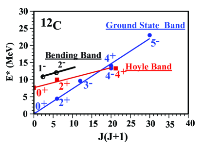
Figure 16: (Color Online) Rotational band structure of the ground-state band, the Hoyle band and the bending vibration in ¹²C.

Fig. 16 shows that both the ground state rotational band and the Hoyle band follow a $J(J+1)$ trajectory albeit with a different moment of inertia. The moment of inertia of the bending vibration is almost the same as that of the Hoyle band.

Fig. 17 shows a comparison between experimental and theoretical form factors. The coefficient $\beta$ is determined from the first minimum in the elastic form factor to be $\beta=1.74$ fm, and subsequently the coefficient $\alpha$ is obtained from the charge radius of ¹²C to be $\alpha=0.52$ fm^-2. The $q$ dependence of the form factors is consistent with experiment, indicating that the $2^{+}_{1}$ and $0^{+}_{2}$ states can be interpreted as rotational and vibrational excitations of a triangular configuration of three $\alpha$ particles with ${\cal D}_{3h}$ symmetry.

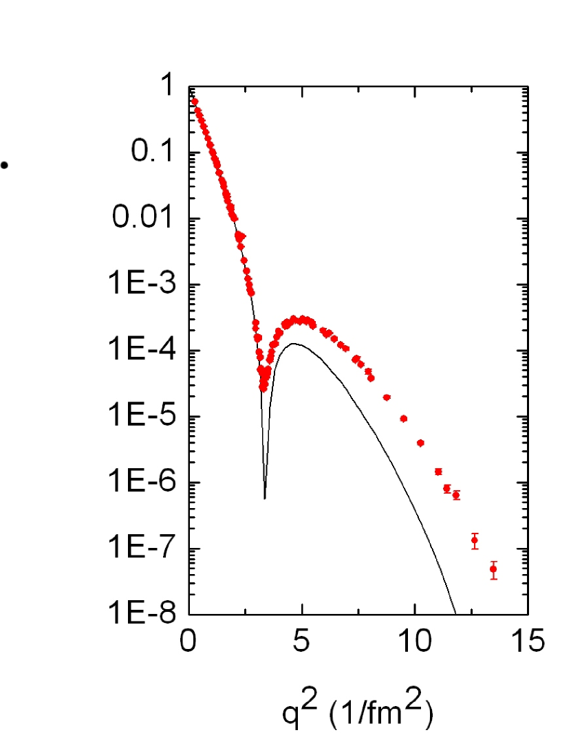
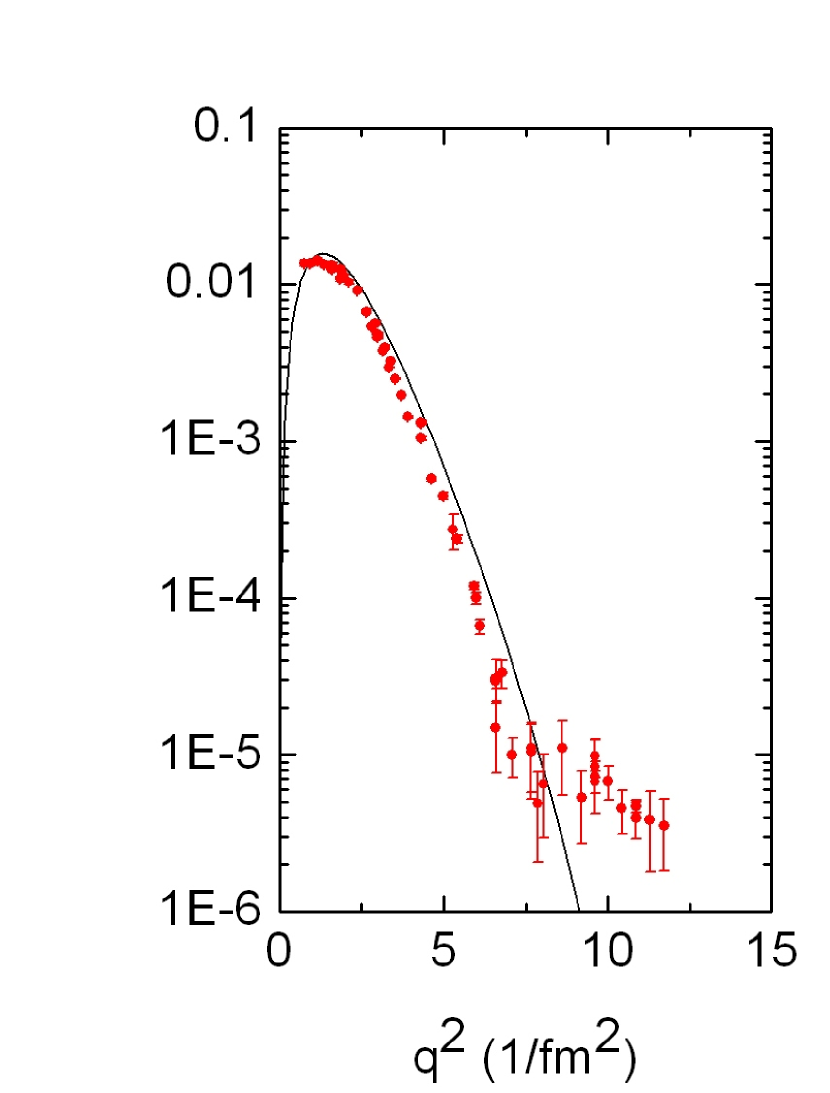
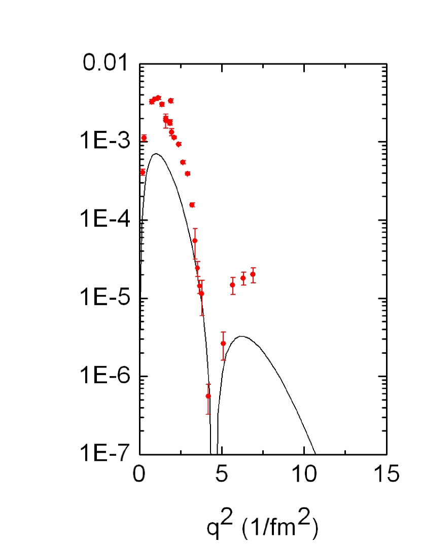
Figure 17: Comparison between the experimental form factors $|{\cal F}(0^{+}_{1}\rightarrow L^{P}_{i};q)|^{2}$ of ¹²C for the final states with $L^{P}_{i}=0^{+}_{1}$, $2^{+}_{1}$ and $0^{+}_{2}$, and those obtained for the oblate top with $N=10$ and $R^{2}=1.40$. The experimental data are taken from [58]-[63].

The $B(EL)$ values can be obtained by taking the long wavelength limit of the form factors according to Eq. (10lmnak). The values extracted from the fit to the form factors are shown in Table 1. The large values of the electromagnetic transitions $B(E2;2_{1}^{+}\rightarrow 0_{1}^{+})$ and $B(E3;3_{1}^{-}\rightarrow 0_{1}^{+})$ indicate a collectivity which is not predicted for simple shell model states. The good agreement for the $B(EL)$ values and the transition form factors for the ground band shows that the positive and negative parity states merge to form a single rotational band. While the $B(E2;2_{1}^{+}\rightarrow 0_{1}^{+})$ and $B(E3;3_{1}^{-}\rightarrow 0_{1}^{+})$ values are in good agreement with experiment, the $B(E2;0_{2}^{+}\rightarrow 2_{1}^{+})$ value deviates by an order of magnitude. This indicates that the $0^{+}_{2}$ Hoyle state cannot be interpreted as a simple vibrational excitation of a rigid triangular configuration of three $\alpha$ particles, but rather corresponds to a more floppy configuration with large rotation-vibration couplings. A more detailed study of the electromagnetic properties of $\alpha$-cluster nuclei in the ACM for non-rigid configurations is in progress [65].

Table 1: Comparison between calculated and measured $B(EL)$ values in ¹²C. Experimental data are taken from [58, 63, 64].

	Th	Exp
$\langle r^{2}\rangle^{1/2}$	2.468	$2.468\pm 0.12$	fm
$M(E0;0_{2}^{+}\rightarrow 0_{1}^{+})$	0.4	$5.5\pm 0.2$	$\mbox{fm}^{2}$
$B(E2;2_{1}^{+}\rightarrow 0_{1}^{+})$	8.4	$7.6\pm 0.4$	$e^{2}\mbox{fm}^{4}$
$B(E3;3_{1}^{-}\rightarrow 0_{1}^{+})$	44	$103\pm 17$	$e^{2}\mbox{fm}^{6}$
$B(E4;4_{1}^{+}\rightarrow 0_{1}^{+})$	73		$e^{2}\mbox{fm}^{8}$

8.2 The nucleus ¹⁶O

Figure 18: Comparison between the low-lying experimental spectrum of ¹⁶O and the energies of the spherical top calculated using Eq. (13). The last column on the left-hand side, shows the lowest observed non-cluster levels with $L^{P}=0^{-}$, $1^{-}$ and $T=0$, $1$.

.

As early as 1954, Dennison suggested that cluster states in ¹⁶O could be understood in terms of an $\alpha$-particle model with ${\cal T}_{d}$ symmetry [66]. This idea was adopted by Kameny [67], Brink [15, 16], and especially by Robson [17]. In recent years, ¹⁶O has been again the subject of several investigations, both within the framework of the no-core shell model [68], ab initio lattice calculations [69] and the algebraic cluster model [33].

In this contribution, the spherical top limit of the $U(10)$ ACM with ${\cal T}_{d}$ symmetry is used to study cluster states in ¹⁶O. Fig. 18 shows a comparison of the cluster states of ¹⁶O with the spectrum of the spherical top with tetrahedral symmetry given by the energy formula

$$E = E_{0}+\omega_{1}(v_{1}+\frac{1}{2})+\omega_{2}(v_{2}+1)$$ (10lmnbedugbgeggipiqisiuiwjb)

$$+\omega_{3}(v_{1}+\frac{3}{2})+\kappa_{(v)}\,L(L+1)~{}.$$

The coefficient $\kappa_{(v)}$ determines the the moments of inertia of the ground state band and the vibrational bands characterized by $(v)=(v_{1}v_{2}v_{3})$. The vibrational energies $\omega_{1}$, $\omega_{2}$ and $\omega_{3}$ are obtained from the excitation energies of the first excited $0^{+}$, $2^{+}$ and $1^{-}$ states, respectively.

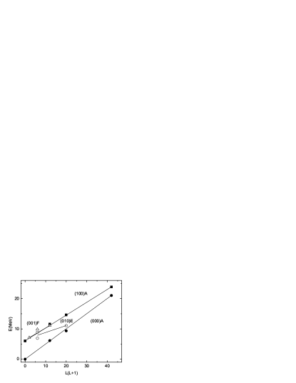
Figure 19: The excitation energies of cluster states in ¹⁶O plotted as a function of $L(L+1)$: closed circles for the ground state band, closed squares for the $A$ vibration, open circles for the $E$ vibration and open triangles for the $F$ vibration.

For the ground state rotational band the states with angular momentum and parity $L^{P}=0^{+}$, $3^{-}$, $4^{+}$, $6^{+}$ have been observed, only the $6^{-}$ state is missing. Another sequence of states $0^{+}$, $3^{-}$, $4^{+}$, $6^{+}$ has been identified as a candidate for the symmetric stretching or breathing vibration $(100)A$ with a somewhat larger moment of inertia than the ground state band which is to be expected for a breathing vibration. All three fundamental vibrations, $(100)A$, $(010)E$ and $(001)F$, have been observed with comparable energies, $\sim 6$ MeV. The band structure is summarized in Fig. 19.

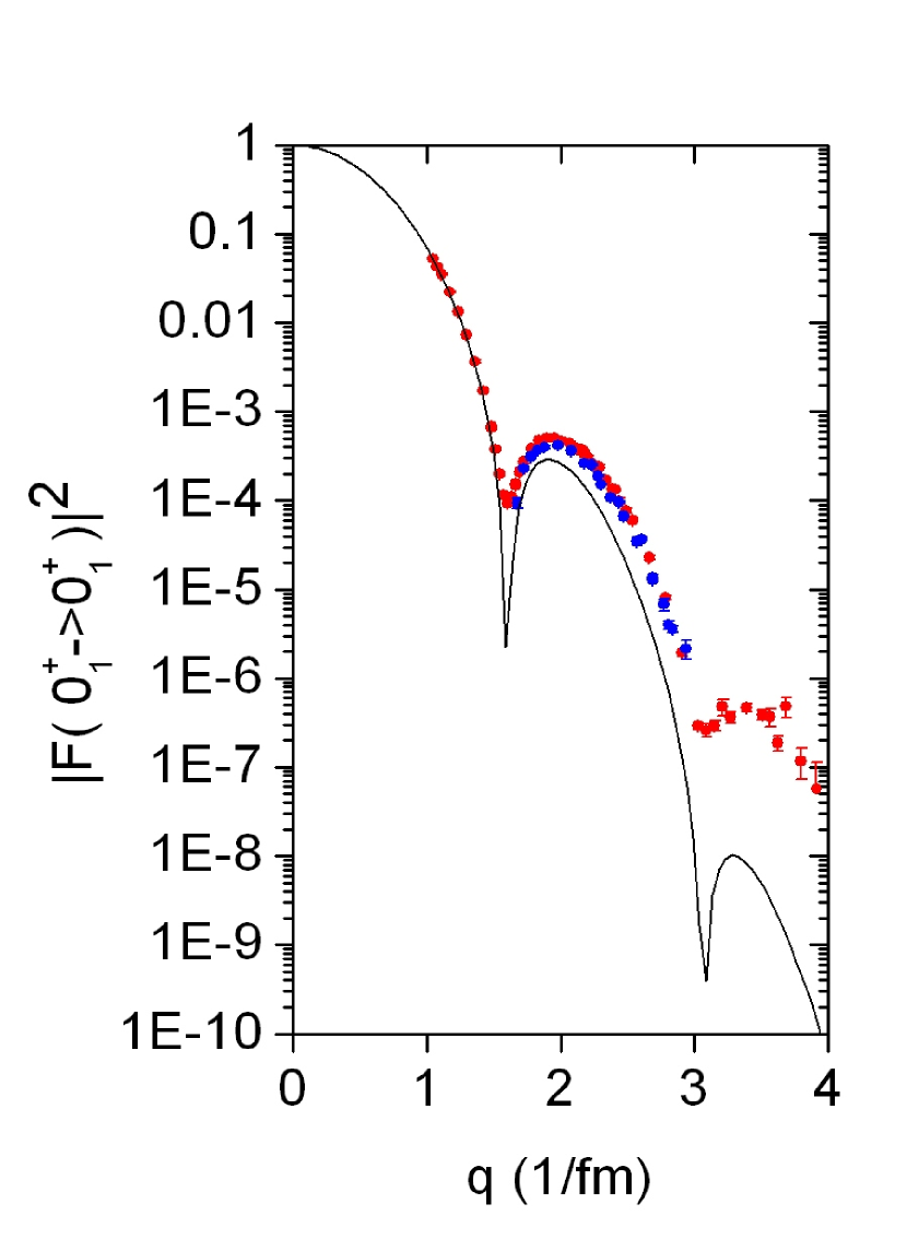
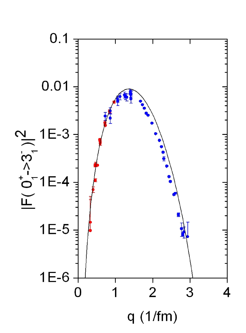
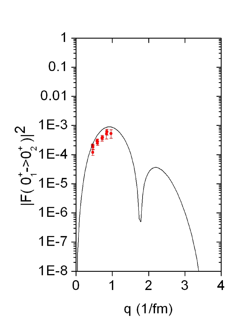
Figure 20: Comparison between the experimental form factors $|{\cal F}(0_{1}^{+}\rightarrow L^{P}_{i})|^{2}$ of ¹⁶O for the final states with $L^{P}_{i}=0^{+}_{1}$, $3^{-}_{1}$ and $0^{+}_{2}$ and those obtained for the spherical top with $N=10$ and $R^{2}=1.0$. The experimental data are taken from Refs. [59, 61, 70, 71, 72].

After having identified the cluster states, the ${\cal T}_{d}$ symmetry can be tested further by means of electromagnetic form factors and $B(EL)$ values. The value of $\beta$ was determined from the first minimum in the elastic form factor to be $\beta=2.071$ fm, and subsequently the value of $\alpha=0.605$ fm^-2 from the charge radius. Fig. 20 shows a comparison between experimental and calculated form factors. The experimental data for the excitation of the $3^{-}_{1}$ state (red) [70, 71] are combined with those of the unresolved doublet of the $3^{-}_{1}$ and $0^{+}_{2}$ states at 6.1 MeV (blue) [61, 72]. Table 2 shows the results for the $B(EL)$ values.

Table 2: Comparison between calculated and measured $B(EL)$ values in ¹⁶O. The experimental values are taken from [73].

	Th	Exp
$\langle r^{2}\rangle^{1/2}$	2.710	$2.710\pm 0.015$	fm
$M(E0;0_{2}^{+}\rightarrow 0_{1}^{+})$	0.54	$3.55\pm 0.21$	$\mbox{fm}^{2}$
$B(E3;3_{1}^{-}\rightarrow 0_{1}^{+})$	215	$205\pm 10$	$e^{2}\mbox{fm}^{6}$
$B(E4;4_{1}^{+}\rightarrow 0_{1}^{+})$	425	$378\pm 133$	$e^{2}\mbox{fm}^{8}$
$B(E6;6_{1}^{+}\rightarrow 0_{1}^{+})$	9626		$e^{2}\mbox{fm}^{12}$

In conclusion, the evidence for the occurrence of the tetrahedral symmetry in the low-lying spectrum of ¹⁶O presented long ago by Dennison [66], Kameny [67] and Robson [17]. was confirmed in a study of the energy spectrum in the ACM for four-body clusters albeit with some differences in the assignments of the states. A study of $B(EL)$ values along the ground state band provides additional evidence for ${\cal T}_{d}$ symmetry. Finally, the results presented here for ¹²C and ¹⁶O emphasize the occurrence of $\alpha$-cluster states in light nuclei with ${\cal D}_{3h}$ and ${\cal T}_{d}$ point group symmetries, respectively.

9 Summary and conclusions

In this contribution, I presented a review of the algebraic cluster model for two-, three- and four-body clusters. The ACM is an interacting boson model that describes the relative motion of cluster configurations in which all vibrational and rotational degrees of freedom are present from the outset. Special attention was paid to the case of identical clusters, and the consequences of their geometrical configuration on the structure of rotational bands (for a summary see Table 3). For three identical clusters located at the vertices of an equilateral triangle, the ground state rotational band has $L^{P}=0^{+}$, $2^{+}$, $3^{-}$, $4^{\pm}$, $5^{-}$, $\ldots$, all of which have been observed in ¹²C. For four identical clusters located at the vertices of a tetrahedron, the sequence is given by $L^{P}=0^{+}$, $3^{-}$, $4^{+}$, $6^{\pm}$, $\ldots$. With the exception of the $6^{-}$ state, all have been observed in ¹⁶O.

Table 3: Algebraic Cluster Model

	$2\alpha$	$3\alpha$	$4\alpha$
ACM	$U(4)$	$U(7)$	$U(10)$
Point group	${\cal C}_{2}$	${\cal D}_{3h}$	${\cal T}_{d}$
Geom. conf.	Linear	Triangle	Tetrahedron
Model	Rotor	Obl. top	Sph. top
Vibrations	$1$	$3$	$6$
Rotations	$2$	$3$	$3$
G.s. band	$0^{+}$	$0^{+}$	$0^{+}$
	$2^{+}$	$2^{+}$
		$3^{-}$	$3^{-}$
	$4^{+}$	$4^{\pm}$	$4^{+}$
		$5^{-}$
	$6^{+}$	$6^{\pm+}$	$6^{\pm}$

The structure of the rotational bands can be considered as the fingerprint of the underlying geometrical cluster configuration. Whereas most theoretical models and ab initio calculations agree on a triangular configuration of $\alpha$ particles for the ground state band in ¹²C [20, 30, 32] and a tetrahedral configuration for the ground state band in ¹⁶O [33, 69], important differences are found in the predictions for the structure of the rotational band built on the first excited $0^{+}$ state. The so-called Hoyle band in ¹²C, i.e. the rotational excitations of the Hoyle state, is of particular interest [57]. While the observed moment of inertia of the Hoyle band excludes the proposed linear chain structure of the Hoyle state [74], there are two alternatives for the geometrical arrangement of the three alpha particles in the Hoyle state of ¹²C, either an equilateral triangular arrangement [20, 32] or a bent-arm configuration as suggested by EFT lattice calculations [30]. In order to distinguish between these two different geometrical configurations of the Hoyle band, the identification of the negative parity states $3^{-}$ and $4^{-}$ is crucial. The selectivity of $\gamma$-ray beams as well as electron beams could help to populate the states of interest and resolve the broad interfering states. These new capabilities should initiate an extensive experimental program for the search of the predicted (“missing”) states and promises to shed new light on the clustering phenomena in light nuclei.

A similar situation exists for the first excited $0^{+}$ state in ¹⁶O. Whereas the ACM is based on a tetrahedral configuration of the $\alpha$ particles, ab initio lattice calculations suggested a square configuration [69]. The latter configuration would imply a large breaking of the ${\cal T}_{d}$ symmetry for the vibrations in Fig. 18.

As a final remark, the ACM is able to account for many different geometrical configurations other than the rigid structures for identical clusters as discussed in this contribution. It can be applied both for identical and non-identical clusters, and for rigid and floppy structures. One of the most challenging problems in clustering in nuclei is to understand what type of configurations are present, and to provide unambiguous experimental evidence for these configurations. The algebraic method provides a general theoretical framework in which calculations can be performed easily in a clear and transparent manner.

Appendix A Triangular symmetry

There are three different symmetry classes for the permutation of three objects. Due to the isomorphism with the dihedral group $S_{3}\sim{\cal D}_{3}$, the three symmetry classes can also be labeled by the irreducible representations of the point group ${\cal D}_{3}$ as $[3]\sim A_{1}$, $[21]\sim E$, and $[111]\sim A_{2}$, with dimensions 1, 2 and 1, respectively.

The permutation symmetry can be determined by considering the transposition $P(12)$ and the cyclic permutation $P(123)$. The transformation properties of the three different symmetry classes under $P(12)$ and $P(123)$ are given by

$$P(12)\left(\begin{array}[]{c}\psi_{A_{1}}\\ \psi_{A_{2}}\end{array}\right)=\left(\begin{array}[]{rr}1&0\\ 0&-1\end{array}\right)\left(\begin{array}[]{c}\psi_{A_{1}}\\ \psi_{A_{2}}\end{array}\right),$$ (10lmnbedugbgeggipiqisiuiwji)

$$P(12)\left(\begin{array}[]{c}\psi_{E_{\rho}}\\ \psi_{E_{\lambda}}\end{array}\right)=\left(\begin{array}[]{rr}-1&0\\ 0&1\end{array}\right)\left(\begin{array}[]{c}\psi_{E_{\rho}}\\ \psi_{E_{\lambda}}\end{array}\right),$$ (10lmnbedugbgeggipiqisiuiwjp)

and

$$P(123)\left(\begin{array}[]{c}\psi_{A_{1}}\\ \psi_{A_{2}}\end{array}\right)=\left(\begin{array}[]{cc}1&0\\ 0&1\end{array}\right)\left(\begin{array}[]{c}\psi_{A_{1}}\\ \psi_{A_{2}}\end{array}\right),$$ (10lmnbedugbgeggipiqisiuiwjw)

$$P(123)\left(\begin{array}[]{c}\psi_{E_{\rho}}\\ \psi_{E_{\lambda}}\end{array}\right)=\left(\begin{array}[]{cc}-\frac{1}{2}&\frac{\sqrt{3}}{2}\\ -\frac{\sqrt{3}}{2}&-\frac{1}{2}\end{array}\right)\left(\begin{array}[]{c}\psi_{E_{\rho}}\\ \psi_{E_{\lambda}}\end{array}\right).$$ (10lmnbedugbgeggipiqisiuiwkd)

Appendix B Tetrahedral symmetry

There are five different symmetry classes for the permutation of four objects. Due to the isomorphism with the tetrahedral group $S_{4}\sim{\cal T}_{d}$, the five symmetry classes can also be labeled by the irreducible representations of the point group ${\cal T}_{d}$ as $[4]\sim A_{1}$, $[31]\sim F_{2}$, $[22]\sim E$, $[211]\sim F_{1}$ and $[1111]\sim A_{2}$, with dimensions 1, 3, 2, 3 and 1, respectively.

The permutation symmetry can be determined by considering the transposition $P(12)$ and the cyclic permutation $P(1234)$. The transformation properties of the five different symmetry classes under $P(12)$ and $P(1234)$ are given by

$$P(12)\left(\begin{array}[]{c}\psi_{A_{1}}\\ \psi_{A_{2}}\end{array}\right) = \left(\begin{array}[]{rr}1&0\\ 0&-1\end{array}\right)\left(\begin{array}[]{c}\psi_{A_{1}}\\ \psi_{A_{2}}\end{array}\right),$$ (10lmnbedugbgeggipiqisiuiwkk)

$$P(12)\left(\begin{array}[]{c}\psi_{E_{\rho}}\\ \psi_{E_{\lambda}}\end{array}\right) = \left(\begin{array}[]{rr}-1&0\\ 0&1\end{array}\right)\left(\begin{array}[]{c}\psi_{E_{\rho}}\\ \psi_{E_{\lambda}}\end{array}\right),$$ (10lmnbedugbgeggipiqisiuiwkr)

$$P(12)\left(\begin{array}[]{c}\psi_{F_{2\rho}}\\ \psi_{F_{2\lambda}}\\ \psi_{F_{2\eta}}\end{array}\right) = \left(\begin{array}[]{rrr}-1&0&0\\ 0&1&0\\ 0&0&1\end{array}\right)\left(\begin{array}[]{c}\psi_{F_{2\rho}}\\ \psi_{F_{2\lambda}}\\ \psi_{F_{2\eta}}\end{array}\right),$$ (10lmnbedugbgeggipiqisiuiwlb)

$$P(12)\left(\begin{array}[]{c}\psi_{F_{1\rho}}\\ \psi_{F_{1\lambda}}\\ \psi_{F_{1\eta}}\end{array}\right) = \left(\begin{array}[]{rrr}1&0&0\\ 0&-1&0\\ 0&0&-1\end{array}\right)\left(\begin{array}[]{c}\psi_{F_{1\rho}}\\ \psi_{F_{1\lambda}}\\ \psi_{F_{1\eta}}\end{array}\right),$$ (10lmnbedugbgeggipiqisiuiwll)

and

$$P(1234)\left(\begin{array}[]{c}\psi_{A_{1}}\\ \psi_{A_{2}}\end{array}\right) = \left(\begin{array}[]{cc}1&0\\ 0&1\end{array}\right)\left(\begin{array}[]{c}\psi_{A_{1}}\\ \psi_{A_{2}}\end{array}\right),$$ (10lmnbedugbgeggipiqisiuiwlt)

$$P(1234)\left(\begin{array}[]{c}\psi_{E_{\rho}}\\ \psi_{E_{\lambda}}\end{array}\right) = \left(\begin{array}[]{cc}\frac{1}{2}&-\frac{\sqrt{3}}{2}\\ -\frac{\sqrt{3}}{2}&-\frac{1}{2}\end{array}\right)\left(\begin{array}[]{c}\psi_{E_{\rho}}\\ \psi_{E_{\lambda}}\end{array}\right),$$ (10lmnbedugbgeggipiqisiuiwma)

$$P(1234)\left(\begin{array}[]{c}\psi_{F_{2\rho}}\\ \psi_{F_{2\lambda}}\\ \psi_{F_{2\eta}}\end{array}\right)$$ (10lmnbedugbgeggipiqisiuiwmf)

$$\hskip 28.45274pt=\left(\begin{array}[]{ccc}-\frac{1}{2}&\frac{\sqrt{3}}{2}&0\\ -\frac{1}{2\sqrt{3}}&-\frac{1}{6}&\frac{\sqrt{8}}{3}\\ -\frac{\sqrt{2}}{\sqrt{3}}&-\frac{\sqrt{2}}{3}&-\frac{1}{3}\end{array}\right)\left(\begin{array}[]{c}\psi_{F_{2\rho}}\\ \psi_{F_{2\lambda}}\\ \psi_{F_{2\eta}}\end{array}\right),$$ (10lmnbedugbgeggipiqisiuiwmm)

$$P(1234)\left(\begin{array}[]{c}\psi_{F_{1\rho}}\\ \psi_{F_{1\lambda}}\\ \psi_{F_{1\eta}}\end{array}\right)$$ (10lmnbedugbgeggipiqisiuiwmq)

$$\hskip 28.45274pt=\left(\begin{array}[]{ccc}\frac{1}{2}&-\frac{\sqrt{3}}{2}&0\\ \frac{1}{2\sqrt{3}}&\frac{1}{6}&-\frac{\sqrt{8}}{3}\\ \frac{\sqrt{2}}{\sqrt{3}}&\frac{\sqrt{2}}{3}&\frac{1}{3}\end{array}\right)\left(\begin{array}[]{c}\psi_{F_{1\rho}}\\ \psi_{F_{1\lambda}}\\ \psi_{F_{1\eta}}\end{array}\right).$$ (10lmnbedugbgeggipiqisiuiwmx)

References

References

- [1] Heisenberg W 1932 Z. Phys. 77 1
- [2] Wigner E P 1937 Phys. Rev. 51 106
- [3] Racah G 1943 Phys. Rev. 43 367
- [4] Talmi I 1971 Nucl. Phys. A 172 1
- [5] Elliott J P 1958 Proc. Roy. Soc. (London) A 245 128 and 562
- [6] Iachello F and Arima A 1987 The Interacting Boson Model (Cambridge: Cambridge U. Press)
- [7] Goeppert-Mayer M 1949 Phys. Rev.75 1969
- [8] Haxel O, Jensen J H D and Suess H E 1949 Phys. Rev. 75 1766
- [9] Bohr A and Mottelson B R 1975 Nuclear Structure Volume II: Nuclear Deformations (Reading, Massachusetts: W. A. Benjamin, Inc.)
- [10] Van Isacker P and Pittel S 2016 Phys. Scr. 91 023009
-
[11]
Dudek J, Goźdź A, Schunck N and Miśkiewicz 2002 Phys. Rev. Lett. 88 252502
Dudek J, Curien D, Dubray N, Dobaczewski J, Pangon V, Olbratowski P and Schunck N 2006 Phys. Rev. Lett. 97 072501 - [12] Van Isacker P, Bouldjedri A and Zerguine S 2015 Nucl. Phys. A 938 45
- [13] Wheeler J A 1937 Phys. Rev. 52 1083
- [14] Hafstad L R and Teller E 1938 Phys. Rev. 54 681
- [15] Brink D M 1965 Int. School of Physics Enrico Fermi, Course XXXVI 247
- [16] Brink D M, Friedrich H, Weiguny A and Wong C W 1970 Phys. Lett. B 33 143
-
[17]
Robson D 1978 Nucl. Phys. A 308 381
Robson D 1979 Phys. Rev. Lett. 42 876
Robson D 1982 Phys. Rev. C 25 1108
Robson D 1982 Prog. Part. Nucl. Phys. 8 257 - [18] Freer M and Fynbo H O U 2014 Prog. Part. Nucl. Phys. 78 1
-
[19]
Freer M et al. 2007 Phys. Rev. C 76 034320
Kirsebom O S et al. 2010 Phys. Rev. C 81 064313 - [20] Marín-Lámbarri D J, Bijker R, Freer M, Gai M, Kokalova T, Parker D J and Wheldon C 2014 Phys. Rev. Lett. 113 012502 (arXiv:1405.7445)
- [21] Itoh M et al. 2011 Phys. Rev. C 84 054308
- [22] Freer M et al. 2012 Phys. Rev. C 86 034320
- [23] Zimmerman W R et al. 2013 Phys. Rev. Lett. 110 152502
- [24] Freer M et al. 2011 Phys. Rev. C 83 034314
-
[25]
Cseh J 1992 Phys. Lett. B 281 173
Cseh J and Lévai G 1994 Ann. Phys. (N.Y.) 230 165
Cseh J and Trencsényi R 2016 arXiv:1604.03123 - [26] Kanada-En’yo Y 2007 Prog. Theor. Phys. 117 655
- [27] Chernykh M, Feldmeier H, Neff H, Von Neumann-Cosel P and Richter A 2007 Phys. Rev. Lett. 98 032501
- [28] Funaki Y, Horiuchi H, Von Oertzen W, Ropke G, Schuck P, Tohsaki A and Yamada T 2009 Phys. Rev. C 80 64326
- [29] Roth R, Langhammer J, Calci A, Binder S and Navratil P 2011 Phys. Rev. Lett. 107 072501
-
[30]
Epelbaum E, Krebs H, Lee D and Meissner U G 2011 Phys. Rev. Lett. 106 192501
Epelbaum E, Krebs H, Lähde T A, Lee D, and Meissner U G 2012 Phys. Rev. Lett. 109 252501 - [31] Dreyfuss A C, Launey K D, Dytrych T, Draayer J P and Bahri C 2013 Phys. Lett. B 727 511
-
[32]
Bijker R and Iachello F 2000 Phys. Rev. C 61 067305
Bijker R and Iachello F 2002 Ann. Phys. (N.Y.) 298 334 -
[33]
Bijker R and Iachello F 2014 Phys. Rev. Lett. 112 152501 (arXiv:1403.6773)
Bijker R and Iachello F 2016 in preparation - [34] Jackson J D 1962 Classical Electrodynamics (New York: Wiley)
- [35] Iachello F and Levine R D 1995 Algebraic Theory of Molecules (Oxford: Oxford U. Press)
-
[36]
Iachello F and Jackson AD 1982 Phys. Lett. B 108 151
Iachello F 1983 Nucl. Phys. A 396 233c
Daley H J and Iachello F 1983 Phys. Lett. B 131 281 -
[37]
Iachello F, Mukhopadhyay N C and Zhang L 1991 Phys. Rev. D 44 898
Iachello F and Kusnezov D 1992 Phys. Rev. D 45 4156 -
[38]
Bijker R, Iachello F and Leviatan A 1994 Ann. Phys. (N.Y.) 236 69
Bijker R, Iachello F and Leviatan A 2000 Ann. Phys. (N.Y.) 284 89 - [39] Bijker R, Dieperink A E L and Leviatan A 1995 Phys. Rev. A 52 2786
-
[40]
Bijker R 2010 AIP Conf. Proc. 1323 28
Bijker R 2012 J. Phys.: Conf. Ser. 380 012003 - [41] Kramer P and Moshinsky M 1966 Nucl. Phys. 82 241
- [42] Coxeter H S M 1973 Regular polytopes (New York: Dover)
- [43] Van Roosmalen O S and Dieperink A E L 1982 Ann. Phys. (N.Y.) 139 198
- [44] Levit S and Smilansky U 1982 Nucl. Phys. A 389 56
- [45] Bohr A and Mottelson B R 1980 Physica Scripta 22 468
- [46] Ginocchio J N and Kirson M 1980 Phys. Rev. Lett. 44 1744
- [47] Dieperink A E L, Scholten O and Iachello F 1980 Phys. Rev. Lett. 44 1747
- [48] Van Roosmalen O S 1982 Ph.D. Thesis (University of Groningen: unpublished)
- [49] De Forest Jr. T and Walecka J D 1966 Advances in Physics 15 1
- [50] Bijker R 2015 Physica Scripta 90 074006 (arXiv:1412.5552)
- [51] Iachello F 1981 Chem. Phys. Lett. 78 581
- [52] Bijker R, Amado R D and Sparrow D A 1986 Phys. Rev. A 33 871
- [53] Talmi I 1952 Helv. Phys. Acta 25 185
- [54] Moshinksy M 1959 Nucl. Phys. 13 104
- [55] Dobeš J 1977 J. Phys. A: Math. Gen. 10 2053
- [56] Herzberg G 1991 Molecular Spectra and Molecular Structure. II. Infrared and Raman Spectra of Polyatomic Molecules (Malabar Florida: Krieger).
- [57] Fynbo H O U and Freer M 2011 Viewpoint, Physics 4 94
- [58] Reuter W, Fricke G, Merle K and Miska H 1982 Phys. Rev. C 26 806
- [59] Sick I and McCarthy J S 1970 Nucl. Phys. A 150 631
- [60] Crannell H L and Griffy T A 1964 Phys. Rev. 136 B1580
- [61] Crannell H 1966 Phys. Rev. 148 1107
- [62] Crannell H, O’Brien J T and Stober D I 1979 Int. Conf. on Nuclear Physics with Electromagnetic Interactions (Mainz)
- [63] Strehl P and Schucan Th H 1968 Phys. Lett. 27B 641
- [64] Ajzenberg-Selove F 1990 Nucl. Phys. A 506 1
- [65] Bijker R 2016 Work in progress
- [66] Dennison D M 1954 Phys. Rev. 96 378
- [67] Kameny S L 1956 Phys. Rev. 103 358
- [68] Navrátil P 2007 Proc. Int. School of Physics “Enrico Fermi”, Course CLXIX arXiv:0711.2702, and references therein.
- [69] Epelbaum E, Krebs H, Lähde T A, Lee D, Meissner U G and Rupak G 2014 Phys. Rev. Lett. 112 102501
- [70] Bergstrom J C, Bertozzi W, Kowalski S, Maruyama X K, Lightbody Jr. J W, Fivozinsky S P and Penner S 1970 Phys. Rev. Lett. 24 152
- [71] Stroetzel M 1968 Z. Phys. 214 357 .
- [72] Bishop G R, Betourne C and Isabelle D B 1964 Nucl. Phys. 53 366
- [73] Tilley D R, Weller H R and Cheves C M 1993 Nucl. Phys. A 564 1
- [74] Morinaga H 1956 Phys. Rev. 101 254