Fluctuations of a surface relaxation model in interacting scale free networks

Abstract

Isolated complex networks have been studied deeply in the last decades due to the fact that many real systems can be modeled using these types of structures. However, it is well known that the behavior of a system not only depends on itself, but usually also depends on the dynamics of other structures. For this reason, interacting complex networks and the processes developed on them have been the focus of study of many researches in the last years. One of the most studied subjects in this type of structures is the Synchronization problem, which is important in a wide variety of processes in real systems. In this manuscript we study the synchronization of two interacting scale-free networks, in which each node has $ke$ dependency links with different nodes in the other network. We map the synchronization problem with an interface growth, by studying the fluctuations in the steady state of a scalar field defined in both networks.

We find that as $ke$ slightly increases from $ke=0$, there is a really significant decreasing in the fluctuations of the system. However, this considerable improvement takes place mainly for small values of $ke$, when the interaction between networks becomes stronger there is only a slight change in the fluctuations. We characterize how the dispersion of the scalar field depends on the internal degree, and we show that a combination between the decreasing of this dispersion and the integer nature of our growth model are the responsible for the behavior of the fluctuations with $ke$.

I Introduction

In the last decades the study of complex networks has attracted the attention of many researchers because many real processes evolve on these types of structures. In early stages of these studies researchers were focused on processes that develop on isolated networks, however, systems, in general, are not completely isolated, but interacting with other systems instead. These types of interacting systems, which are a special case of the class called Networks of Networks (NoN), are composed of internal and external connections. NoN structures were successfully used to understand epidemic spreading [3, 1, 2, 4, 5], cascade of failures [8, 7, 9, 6, 5, 4], diffusion [11, 5, 4, 10] and synchronization [4, 15, 13, 12, 14].

Synchronization phenomena is a relevant subject in many areas, such as in neurobiology [15, 17, 19, 16, 18], animal behavior [20, 22, 21], power-grid networks [23, 24, 25] and so forth. In a relatively recent approach, synchronization problems in complex networks are associated to the fluctuations of a scalar $h$ defined over the system [34, 37, 36, 39, 38, 28, 26, 32, 33, 31, 29, 27, 30, 35, 14]. This scalar field is a measure of the amount of load that a node has to manage. For example, in the problem of queuing networks, the load is proportional to the waiting time that a node needs to complete his task. The load in a node must be reduced in order to avoid increasing the waiting time by distributing efficiently the loads and thus improving the synchronization. In this approach the fluctuations are given by

$$W=\sqrt{\left\{\frac{1}{N}\sum_{i=1}^{N}(h_{i}-\langle h\rangle)^{2}\right\}}\ ,$$ (1)

where $h_{i}$ is the load of node $i$, $\langle h\rangle$ is the average value of the load over the network, $N$ is the system size, and $\{\}$ is the statistical average. In the steady state the fluctuations reach a constant value $W\equiv W_{s}$, which depends on the topology of the network. This type of process was studied in networks with different topologies, but in the last few years many researches have focused on Scale-Free (SF) networks because they are obiquous in many real systems. These kinds of networks are characterized by a degree distribution $P(k)\sim k^{-\lambda}$, where $P(k)$ is the probability that a node has $k$ internal links and $\lambda$ is the exponent of the power law distribution. In general, $\lambda$ takes values between $2.5$ and $3$ in real SF networks.

One of the most studied models of growth interface is the Family model [40, 37, 36, 39, 38, 35, 14], which is a surface relaxation model (SRM). In this model, at each time-step a node is randomly chosen, and the node with the lowest amount of load or ‘height’ between the selected node and its neighbors increases its load in one unit. In isolated SF networks with exponent $\lambda<3$ it was found that the dependence of $W_{s}$ with the system size $N$ has a crossover between two different behaviors at a characteristic size $N_{0}$: for $N<N_{0}$, $W_{s}\sim logN$ , and $W_{s}$ $\sim$ constant for $N>N_{0}$ [35]. Thus in the last regime the system is scalable, i.e. increasing the system size does not affect the fluctuations. In a more recent work [14] the authors studied the SRM in two interacting SF networks, in which a fraction $q$ ($0\leq q\leq 1$) of nodes in each network is connected one by one through bidirectional external links, allowing diffusion from one network to another. They found that the synchronization improves as $q$ increases and reaches an improvement of $40\%$ for $q=1$. In real systems however, nodes can have more than one external connection with nodes in the other networks, which implies a stronger interaction between the systems. This strong interaction may affect the processes that develop on structures of this type. In this work we are interested in understanding how the strong interaction between networks affects the synchronization of the system. For this purpose we study the SRM model in two SF networks in which each node has $ke$ external connections. In this study we only use stochastic simulations due to the fact that the heterogeneity of the SF networks and the lack of geometrical direction makes difficult any theoretical approach [36].

II Model

We build two SF networks $A_{i}$ ($i=1,2$) using the Molloy–Reed Algorithm [41], avoiding multiple and self connections, and we use a minimum degree $k_{min}=2$ to ensure that each network has a single component [42]. In both networks every node $j$, with $j=1,..,N$, has $k_{j}^{i}$ internal connections with nodes in the same network and $ke$ external connections with nodes in the other network. By simplicity, we consider the same number of external connections for all nodes. We denote by $v_{j}^{i}$ and $b_{j}^{i}$ the set of internal and external neighboring nodes respectively of node $j$ from network $A_{i}$. We chose as initial condition all the scalar fields $h_{j}^{i}$ randomly distributed in the interval $[0,1]$.

At each time step a node $j$ in one of the networks $A_{i}$, with $i=1,2$, is randomly chosen and receives a load unit. Then:

1) The load diffuses to the node $m$, which is the one with the smaller load in the set $\{j,v_{j}^{i}\}$. We denote this process as the first internal diffusion.

2) If $h_{m}^{i}$ is smaller than all the heights in the set $b_{m}^{i}$, then the load is deposited in $m$ and $h_{m}^{i}=h_{m}^{i}+1$. (color green in Fig 1). Otherwise the load diffuses to the node with the smaller height in the set $\{b_{m}^{i}\}$ . We denote this process as external diffusion.

3) If an external diffusion takes place, step $1)$ is repeated and, after a second internal diffusion, the load is deposited in a node $n$ in the network $A_{l}$ with $l\neq i$ (color red in Fig 1). Then $h_{n}^{l}=h_{n}^{l}+1$.

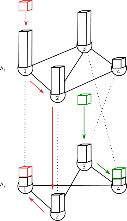
Figure 1: Schematic of the rules of our model for two interacting networks. The circles represent the nodes and the columns the amount of load or height in each node. Full lines denote the internal connections and the dot-lines the external ones. The networks have $N=4$ and $ke=1$. A load unit is dropped in a node of one of the networks (colored cubes) and diffuses between nodes following the rules (colored arrows), until it is finally deposited.

III Results and Discussions

For the simulations we build two SF networks with the same exponents $\lambda=2.6$ and sizes $N=3\times 10^{5}$ to ensure that the system is in the scalable regime [35]. As the two networks used here have the same exponent $\lambda$ and same system size $N$, the fluctuations $W^{i}_{s}$ on each network will be in average the same, thus by simplicity we drop the index $i$. In Fig. 2 we plot the square fluctuations in the steady state of each network $W^{2}_{s}$ as a function of the external connection parameter $ke$. We can observe that the synchronization of the system improves as $ke$ increases and that the fluctuations converge asymptotically to the optimal value $W_{s}^{2}(N)$, which corresponds to the case $ke=N$. The reduction in the fluctuations when more external connections are added is due to the fact that the overloaded nodes in one network have the possibility to diffuse their excess of load to nodes that possesess lower levels of load in the other network. This external diffusion allows to synchronize nodes that have increasingly similar amounts of load. It is important to notice that for high interacting networks with $k_{e}=N$, the value $W_{s}^{2}(N)$ is independent of the exponent $\lambda$ of the degree distribution because in this case the interaction between networks, represented by the external connections, dominates the dynamics and the saturation value of the synchronization. Thus in this case of strong interaction the topology of the isolated networks represented by internal connections plays a minor role. More precisely, the nodes have more probability to diffuse to nodes in the other network because the number of external connections is much higher than the number of internal ones.

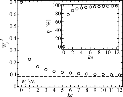
Figure 2: Square fluctuations of the scalar field $W^{2}_{s}$ as a function of the external connections $ke$ ($\circ$). The dashed line corresponds to the case $ke=N$. In the inset we plot the percentage of the maximum improvement that the synchronization can achieve compared to the isolated network $\eta$ as a function of $ke$. For small values of $ke$, $\eta$ almost approaches its optimal value.

In order to visualize the relative improvement of the synchronization compared to the isolated network we compute the percentage of the maximum optimization that the system achieves for $ke>0$, $\eta=(W_{s}^{2}(0)-W_{s}^{2}(ke))/(W_{s}^{2}(0)-W_{s}^{2}(N))\times 100\%$. In the inset of Fig. 2 we plot $\eta$ as function of $ke$. From the plot we can observe that we do not need to have very high values of $ke$ to get a good improvement, since $\eta$ approaches fast to the optimal case ($ke=N$). As $ke$ increases more connections are added in order to obtain some improvement in the synchronization, and this is very expensive compared to the resulting profit. For example, increasing $ke$ from zero to five implies adding $5\;N$ external connections and $\eta$ is about $94.5\%$, when we increase $ke$ from $5$ to $10$ we duplicate the external connections between networks and obtain only a $3\%$ of improvement over the previous case. This is a high cost to pay to only obtain a slight improvement in the synchronization of the system.

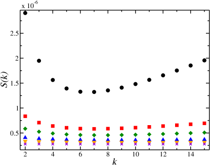
Figure 3: The average contribution $S(k)$ that a node with degree $k$ makes to the fluctuations as a function of $k$, for $ke=0$ (black $\circ$), $ke=1$ (red $\Box$), $ke=2$ (green $\Diamond$), $ke=5$ (blue $\bigtriangleup$), $ke=10$ (orange $\bigtriangledown$), and $ke=N$ (violet $\times$). The values of $S(k)$ shown in the vertical axis are multiplied by $10^{-6}$. The curves exhibit a minimum around $k=6$ for all $ke$. For $ke=N$, $S(k)$ is a constant which does not depend on the topology of the networks.

To understand the role of the internal connections of the nodes in the fluctuations, we define the average contribution $S(k)$ that nodes with degree $k$ made to $W^{2}_{s}$, where $S(k)$ is given by

$$S(k)=\frac{1}{N}\sum_{j=1\;/k_{j}=k}^{N}\frac{(h_{j}-\langle h\rangle)^{2}}{N\;P(k)}\ .$$

It is straightforward to show that $W^{2}_{s}=\sum_{k=k_{min}}^{k_{max}}N\;P(k)\;S(k)$. In Fig. 3 we plot $S(k)$ as a function of the internal degree $k$ for different values of $ke$. From this plot we can see that as $k$ increases $S(k)$ decreases, reaching a minimum around $k=6$. This behavior can be explained as follows: as $k$ increases the nodes have more neighboring nodes to which they can send their excess of load or from which they can receive load, approaching their height to $\langle h\rangle$. However around $k=6$, the nodes have too many neighbors and start to act as load sinks, and thus high degree nodes become the most loaded of the system. As $ke$ increases $S(k)$ decreases for all the values of $k$ and as a consequence the synchronization improves, and in addition $S(k)$ has a minor dependence on $k$. This implies that the amount of load of all the nodes becomes similar and hence the external connections dominate the dynamics of the growth model over the internal topology of the network. Thus $S(k)$ has the same value regardless of the internal degree of a node when $ke=N$. In Fig. 3 we show only the values of $S(k)$ for nodes with $k<15$ because the total contribution from higher degree nodes to the fluctuations is far smaller.

In order to explain why the main contributions to the fluctuations are reduced when the interaction between networks increases, we study the distribution of load of nodes with internal connectivity $k$ around the main value $h(k)-\langle h\rangle$, where $h(k)$ is the average amount of load of nodes with degree $k$. In Fig. 4 we plot the distributions of $h(k)-\langle h\rangle$, for $k=2$ and for $k=10$ for different values of $ke$. From Fig. 4(a), we can see that as the number of external connections increases for $k_{e}>0$, the dispersion of these distributions is reduced. For example, when we increase $ke$ from $0$ to $1$, the dispersion is reduced from $0.934$ to $0.501$. Also these distributions have nodes with levels of load above and below the mean value, and with an average load very close to $\langle h\rangle$, regardless of the value of $ke$. These observations, which are also seen for $k<6$ –not shown here– confirm that the main reason of the reduction of the fluctuations is that nodes with small degree and load above the main value send their excess of load to nodes with also small degree and load below the main value through the external connections of the system. Other values of dispersion of these distributions around the main value are displayed in Table 1.

From Fig. 4(b) we can see that the distribution of $h(k=10)-\langle h\rangle$ for $ke=0$ is not centered in $0$. This is because, as explained above, nodes with $k>6$ act as load sinks and usually become over saturated in the growing process. As $ke$ increases not only the width of the distribution is reduced but also it is centered close to $0$. Thus all the load distributions for different values of $k$ get closer as $ke$ increases. Adding external connections decreases the dispersion of the distributions, however due to the discrete nature of the rules of our growth model and the initial conditions, the reduction has a limit at which the distribution tends to a rectangular shape as can be seen in Fig. 4(a) and Fig. 4(b) for $ke\to N$. Also from Table 1 we can see that the values of the dispersion of the load distribution for $k=2$ are closer to the values for $k=10$ as $ke$ increases. All the results shown in this table are qualitatively the same for other values of $\lambda$ in the interval $2<\lambda\leq 3$.

It is worthwhile to mention that we expect that in NoN composed by more than two networks $W^{2}_{s}$ will be slightly smaller than in the case of two interacting networks, because the system will be able to perform more relaxation steps between networks.

\begin{overpic}[scale={0.25}]{Fig3.eps} \put(20.0,50.0){\bf{(a)}} \end{overpic}

\begin{overpic}[scale={0.25}]{Fig4.eps} \put(20.0,50.0){{\bf{(b)}}} \end{overpic}

Figure 4: (a) Distribution of load of the nodes around the mean value for nodes with (a) degree $k=2$ for $ke=0$ (black $\circ$), $ke=1$ (red $\Box$), $ke=2$ (green $\Diamond$), $ke=5$ (blue $\bigtriangleup$), $ke=10$ (orange $\bigtriangledown$) and $ke=N$ (violet $\times$). (b) degree $k=10$ for $ke=0$ (black $\circ$), $ke=1$ (red $\Box$), $ke=5$ (blue $\bigtriangleup$) and $ke=N$ (violet $\times$).

Table 1: Dispersion of the distributions of load of the nodes with internal degree $k$ around $\langle h\rangle$ for different values of $ke$. Notice that the dispersion is $\sqrt{N\;S(k)}$.

$ke$	0	1	2	5	10	N
$k=2$	0.934	0.501	0.419	0.349	0.317	0.289
$k=10$	0.667	0.427	0.373	0.326	0.306	0.289

IV Conclusions

We studied the synchronization of a system of two interacting SF networks for a simple surface relaxation model, in which the nodes of each network are connected with $ke$ nodes of the other network. We found that as $ke$ increases the synchronization of the system improves, reaching an optimal value for $ke=N$. We also found that the addition of a small number of $ke$ connections results in a similar improvement compared to the case $ke=N$. This is important because an increase in the value of $ke$ requires to add a large number of external connections to the system, which is very expensive from an economic point of view. We explain the reduction of the fluctuations in each network when $ke$ increases, by the decrease of the contributions from nodes with small degree, which is a consequence of the external connections that reduce the dispersion of load of these nodes around the mean value.

In future works we will explore another type of external connection, such as external connections taken from a distribution.

V Acknowledgments

CEL and LAB want to thank UNMdP, FONCyT, Pict 0429/2013, Pict 1407/2014, CONICET, PIP 00443/2014 for financial support. MFT acknowledges CONICET, PIP 00629/2014 for financial support.

References

- [1] Granell C., Gómez S. and Arenas A., Phys. Rev. Lett., 111 (2013) 128701.
- [2] Alvarez-Zuzek L. G., Stanley H. E. and Braunstein L. A., Sci. Rep., 5 (2015) 12151
- [3] Zhao D., Li L., Peng H., Luo Q. and Yang Y., Phys. Lett. A, 378 (2014) 770.
- [4] Boccaletti S., Bianconi G., Criado R., del Genio C. I., Gómez-Gardeñes J., Romance M., Sendiña-Nadal I., Wang Z. and Zanin M., Phys. Rep., 544 (2014) 1-122.
- [5] Kivelä M., Arenas A., Barthelemy M., Gleeson J. P., Moreno Y. and Porter M. A., J. Complex Netw., 2 (2014) 203.
- [6] Valdez L. D., Macri P. A., Stanley H. E. and Braunstein L. A., Phys. Rev. E, 88 (2013) 050803. (R)
- [7] Buldyrev S. V., Parshani R., Paul G. Stanley H. E. and Havlin S., Nature, 464 (2010) 1025.
- [8] Reis S. D. S. , Hu Y., Babino A., Andrade Jr. J. S., Canals S., Sigman M. and Makse H. A., Nat. Phys., 10 (2014) 762.
- [9] D’Agostino G. and Scala A. (Editors), Networks of Networks: The Last Frontier of Complexity (Springer, Rome) 2014.
- [10] De Domenico M., Solé-Ribalta A., Gómez S. and Arenas A., Proc. Natl. Acad. Sci. U.S.A., 111 (2014) 8351.
- [11] Gómez S., Díaz-Guilera A., Gómez-Gardeñes J., Pérez-Vicente C. J., Moreno Y. and Arenas A., Phys. Rev. Lett. 110 (2013) 028701.
- [12] Barreto E., Hunt B., Ott E. and So P., Phys. Rev. E, 77 (2008) 036107.
- [13] Zhang X., Boccaletti S., Guan S. and Liu Z., Phys. Rev. Lett., 114 (2015) 038701.
- [14] Torres M. F., Di Muro M. A., La Rocca C. E. and Braunstein L. A., EPL, 111 (2015) 46001.
- [15] Sun X., Lei J., Perc M., Kurths J. and Chen G., Chaos, 21 (2011) 016110.
- [16] Grinstein G. and Linsker R., Proc. Natl. Acad. Sci. U.S.A., 102 (2005) 9948.
- [17] Guo D., Wang Q. and Perc M., Phys. Rev. E, 85 (2012) 061905.
- [18] Wang Q., Duan Z., Perc M. and Chen G., EPL, 83 (2008) 50008.
- [19] Netoff T. I., Clewley R., Arno S., Keck T. and White J.A., J. Neurosci., 24 (2004) 8075.
- [20] Sun J., Bollt E. M., Porter M. A. and Dawkins M. S., Physica D 240 (2011) 1497.
- [21] Lusseau D., Wilson B., Hammond P. S., Grellier K., Durban J. W., Parsons K. M., Barton T. R. and Thompson P. M., J. Anim. Ecol., 75 (2006) 14.
- [22] Stoye S., Porter M. A. and Dawkins M. S. Livest. Sci., 149 (2012) 70.
- [23] Motter A. E., Myers S. A., Anghel M. and Nishikawa T., Nat. Phys., 9 (2013) 191.
- [24] Rohden M., Sorge A., Timme M. and Witthaut D. Phys. Rev. Lett. 109 (2012) 064101.
- [25] Nishikawa T. and Motter A. E., New J. Phys., 17 (2015) 015012.
- [26] Korniss G., Huang R., Sreenivasan S. and Szymanski B.K., Handbook of Optimization in Complex Networks, edited by Thai M. T. and Pardalos P. M. (Springer, New York) 2011. sect. 3.
- [27] Hunt D., Molnár Jr., Szymanski B.K. and Korniss G., Phys. Rev. E., 92 (2015) 062816.
- [28] Guclu H., Korniss G. and Toroczkai Z., Chaos 17 (2007) 026104.
- [29] Hunt D., Szymanski B. K. and Korniss G., Phys. Rev. E, 86 (2012) 056114.
- [30] Hunt D., Korniss G. and Szymanski B. K., Phys. Rev. Lett., 105 (2010) 068701.
- [31] Toroczkai Z. and Bassler K.E., Nature, 428 (2004) 716.
- [32] Pastore y Piontti A. L., La Rocca C. E., Toroczkai Z., Braunstein L.A., Macri P. A. and López E. D., New J. Phys., 10 (2008) 093007.
- [33] Toroczkai Z., Kozma B., Bassler K. E., Hengartner N. W. and Korniss G., J. Phys. A, 41 (2008) 155103.
- [34] Korniss G., Phys. Rev. E, 75 (2007) 051121.
- [35] Torres D., Di Muro M. A., La Rocca C. E. and Braunstein L. A., EPL, 110 (2015) 66001.
- [36] La Rocca C. E., Braunstein L. A. and Macri P. A., Phys. Rev. E, 77 (2008) 046120.
- [37] Pastore y Piontti A. L., Macri P. A. and Braunstein L. A., Phys. Rev. E, 76 (2007) 046117.
- [38] La Rocca C. E., Braunstein L. A. and Macri P. A., Physica A, 390 (2011) 2840.
- [39] La Rocca C. E., Pastore y Piontti A. L., Braunstein L. A. and Macri P. A., Physica A, 388 (2009) 233.
- [40] Family F., J. Phys. A, 19 (1986) L441.
- [41] Molloy M. and Reed. B., Random Struct. Algorithms, 6 (1995) 161 ; Combin. Probab. Comput., 7 (1998) 295.
- [42] Cohen R., Havlin S. and ben-Avraham D., Handbook of Graphs and Networks, edited by Bornholdt S. and Shuster H. G. (Willey-VCH, New York) (2002), sect. 4.