Conforming restricted Delaunay mesh generation for piecewise smooth complexes

Abstract

A Frontal-Delaunay refinement algorithm for mesh generation in piecewise smooth domains is described. Built using a restricted Delaunay framework, this new algorithm combines a number of novel features, including: (i) an unweighted, conforming restricted Delaunay representation for domains specified as a (non-manifold) collection of piecewise smooth surface patches and curve segments, (ii) a protection strategy for domains containing curve segments that subtend sharply acute angles, and (iii) a new class of off-centre refinement rules designed to achieve high-quality point-placement along embedded curve features. Experimental comparisons show that the new Frontal-Delaunay algorithm outperforms a classical (statically weighted) restricted Delaunay-refinement technique for a number of three-dimensional benchmark problems.

&pdflatex

1 Introduction

Mesh generation is a key component in a variety of mathematical modelling and simulation tasks, including problems in computational engineering, numerical modelling, and computer graphics and animation. Given a general volumetric domain, described by a network of curves $\Gamma\subset\mathbb{R}^{3}$, a collection of surfaces $\Sigma\subset\mathbb{R}^{3}$ and an enclosed volume $\Omega\subset\mathbb{R}^{3}$, the three-dimensional meshing problem consists of tessellating $\Gamma$, $\Sigma$ and $\Omega$ into a mesh of non-overlapping simplexes (edges, triangles and tetrahedrons), such that all geometrical, topological and user-defined constraints are satisfied. While some input domains can be described in terms of smooth entities, it is typical to deal with objects that are only piecewise-smooth, consisting of locally manifold surface patches that meet at sharp 0- or 1-dimensional features. Additionally, input domains can incorporate so-called free curve and vertex constraints, comprising sets of entities unconnected to the bounding surface patches $\Sigma$. In this study, a new Delaunay-refinement type algorithm is presented to construct meshes for piecewise smooth domains – forming a Delaunay tetrahedralisation that includes a subset of restricted edges, triangles and tetrahedrons that provide provably-good topological and geometrical approximations to the input curve network $\Gamma$, surface structure $\Sigma$ and enclosed volume $\Omega$. Using a new class of off-centre refinement rules, the proposed algorithm is cast as a Frontal-Delaunay scheme – seeking to extend the surface- and volume-meshing techniques presented by the author in [1, 2, 3]. Compared to existing restricted Delaunay-refinement techniques, the methods described here incorporate a number of novel features, including: (i) the use of a conforming, unweighted restricted Delaunay representation for piecewise smooth geometries, (ii) the development of a new collar-based method to protect sharply acute features present in the input geometry, and (iii) the use of off-centre point-placement rules to refine curve, surface and volumetric elements in a provably-good manner.

1.1 Nomenclature

The following work is based on the restricted Delaunay framework. The reader is referred to [4] for formal definitions, discussions and proofs.

• $X$: A set of points in $\mathbb{R}^{3}$, associated with the tessellation.

• $\operatorname{Del}\mathopen{}\mathclose{{}\left(X}\right)$: The Delaunay triangulation of the points $X$.

• $\operatorname{Vor}\mathopen{}\mathclose{{}\left(X}\right)$: The Voronoi complex associated with the points $X$.

• $\Gamma,\Sigma,\Omega$: The input geometry: a collection of curve segments, surface patches and volumes embedded in $\mathbb{R}^{3}$.

• $\operatorname{Del}|_{\Gamma}\mathopen{}\mathclose{{}\left(X}\right)$: A Delaunay sub-complex $\operatorname{Del}|_{\Gamma}\mathopen{}\mathclose{{}\left(X}\right)\subseteq\operatorname{Del}\mathopen{}\mathclose{{}\left(X}\right)$, restricted to the curve network $\Gamma$. $\operatorname{Del}|_{\Gamma}\mathopen{}\mathclose{{}\left(X}\right)$ contains any 1-simplex $e\in\operatorname{Del}\mathopen{}\mathclose{{}\left(X}\right)$ whose dual Voronoi face $v_{f}\subseteq\operatorname{Vor}\mathopen{}\mathclose{{}\left(X}\right)$ intersects $\Gamma$ (See Figure 1(ii)–1(iii)).

• $\operatorname{Del}|_{\Sigma}\mathopen{}\mathclose{{}\left(X}\right)$: A Delaunay sub-complex $\operatorname{Del}|_{\Sigma}\mathopen{}\mathclose{{}\left(X}\right)\subseteq\operatorname{Del}\mathopen{}\mathclose{{}\left(X}\right)$, restricted to the surfaces patches $\Sigma$. $\operatorname{Del}|_{\Sigma}\mathopen{}\mathclose{{}\left(X}\right)$ contains any 2-simplex $f\in\operatorname{Del}\mathopen{}\mathclose{{}\left(X}\right)$ whose dual Voronoi edge $v_{e}\subseteq\operatorname{Vor}\mathopen{}\mathclose{{}\left(X}\right)$ intersects $\Sigma$ (See Figure 1(ii)–1(iii)).

• $\operatorname{Del}|_{\Omega}\mathopen{}\mathclose{{}\left(X}\right)$: A Delaunay sub-complex $\operatorname{Del}|_{\Omega}\mathopen{}\mathclose{{}\left(X}\right)\subseteq\operatorname{Del}\mathopen{}\mathclose{{}\left(X}\right)$, restricted to the interior volumes $\Omega$. $\operatorname{Del}|_{\Omega}\mathopen{}\mathclose{{}\left(X}\right)$ contains any 3-simplex $\tau\in\operatorname{Del}\mathopen{}\mathclose{{}\left(X}\right)$ with a dual Voronoi vertex $v_{x}\subseteq\operatorname{Vor}\mathopen{}\mathclose{{}\left(X}\right)$ interior to $\Omega$ (See Figure 1(ii)–1(iii)).

• $\rho_{d}(\tau)$: The radius-edge ratio associated with a $d$-simplex $\tau$. Defined as the ratio of the radius of the circumball of $\tau$ to the length of its shortest edge.

• $\epsilon_{1}(e)$: The surface discretisation error associated with a 1-simplex $e\in\operatorname{Del}|_{\Gamma}\mathopen{}\mathclose{{}\left(X}\right)$. Defined as the length from the centre of $\operatorname{SDB}_{1}(e)$ to the centre of the diametric ball of $e$.

• $\epsilon_{2}(f)$: The surface discretisation error associated with a 2-simplex $f\in\operatorname{Del}|_{\Sigma}\mathopen{}\mathclose{{}\left(X}\right)$. Defined as the length from the centre of $\operatorname{SDB}_{2}(f)$ to the centre of the diametric ball of $f$.

• $\operatorname{SDB}_{1}(e)$: The surface Delaunay ball $B(\mathbf{c}_{e},r)$ associated with a 1-simplex $e\in\operatorname{Del}|_{\Gamma}\mathopen{}\mathclose{{}\left(X}\right)$. Balls are centred at intersections between the Voronoi faces $v_{f}\in\operatorname{Vor}\mathopen{}\mathclose{{}\left(X}\right)$ and the curve network $\Gamma$, such that $\mathbf{c}_{e}=v_{f}\cap\Gamma$.

• $\operatorname{SDB}_{2}(f)$: The surface Delaunay ball $B(\mathbf{c}_{f},r)$ associated with a 2-simplex $f\in\operatorname{Del}|_{\Sigma}\mathopen{}\mathclose{{}\left(X}\right)$. Balls are centred at intersections between the Voronoi edges $v_{e}\in\operatorname{Vor}\mathopen{}\mathclose{{}\left(X}\right)$ and the surface patches $\Sigma$, such that $\mathbf{c}_{f}=v_{e}\cap\Sigma$.

• $\bar{h}(\mathbf{x})$: The mesh-size function. A function $f(\mathbf{x}):\mathbb{R}^{3}\rightarrow\mathbb{R}^{+}$ defining the target edge length at points $\mathbf{x}\in\Omega$.

• $v(\tau)$, $a(f)$: The volume-length and area-length ratios associated with a given tetrahedron $\tau$ or triangle $f$. Defined as $v(\tau)=\nicefrac{{V}}{{\|\mathbf{e}\|^{3}_{\text{rms}}}}$ and $a(f)=\nicefrac{{A}}{{\|\mathbf{e}\|^{2}_{\text{rms}}}}$, where $V$ is the signed volume of $\tau$, $A$ is the signed area of $f$ and $\|\mathbf{e}\|_{\text{rms}}$ is the root-mean-square edge length. The volume-length and area-length ratios are robust measures of tetrahedral and triangular element quality.

1.2 Preliminaries

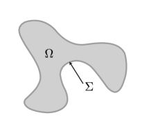
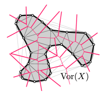
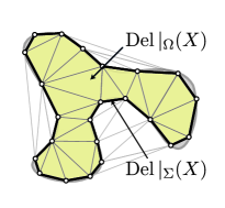
(i)	(ii)	(iii)

Figure 1: Restricted Delaunay tessellations for a smooth domain in $\mathbb{R}^{2}$, showing (i) the bounding contour $\Sigma$ and enclosed interior $\Omega$, (ii) the Delaunay tessellation $\operatorname{Del}\mathopen{}\mathclose{{}\left(X}\right)$ and Voronoi diagram $\operatorname{Vor}\mathopen{}\mathclose{{}\left(X}\right)$, and (iii) the restricted boundary and interior tessellations $\operatorname{Del}|_{\Sigma}\mathopen{}\mathclose{{}\left(X}\right)$ and $\operatorname{Del}|_{\Omega}\mathopen{}\mathclose{{}\left(X}\right)$. In three-dimensions, the restricted surface triangulation $\operatorname{Del}|_{\Sigma}\mathopen{}\mathclose{{}\left(X}\right)$ is a triangular complex that covers the surface $\Sigma$. The restricted volume tessellation $\operatorname{Del}|_{\Omega}\mathopen{}\mathclose{{}\left(X}\right)$ is a tetrahedral complex that fills the volume $\Omega$.

Many successful three-dimensional meshing algorithms employ Delaunay-based strategies [5, 6, 7, 8, 9, 10, 11, 12, 13, 14], based on the progressive refinement of a coarse initial Delaunay triangulation that spans the input geometry. At each step, elements that violate a set of constraints are identified and the worst offending elements are eliminated. Elimination is achieved through the insertion of additional Steiner-vertices located at the so-called refinement-points associated with the elements in question. Delaunay-refinement algorithms have been developed for planar [5, 6, 7], surface [12, 13] and volumetric domains [9, 15, 16]. The reader is referred to [4] for additional information and summary.

This study is focused on use of the so-called restricted Delaunay methodology [17, 11, 14] to provide a framework for the approximation of 1-, 2- and 3-dimensional topological features via Delaunay sub-complexes. Such techniques have been the focus of previous work, including, for example [12, 13, 11, 4] and previous studies by the author in [1, 2, 3], where it has been shown that various geometrical and topological guarantees of fidelity are achieved through a careful sampling of the geometrical inputs. Compared to other approaches, the restricted Delaunay framework incorporates a number of desirable characteristics, chiefly: (i) the ability to sample curve-, surface- and volumetric-features in a unified manner, and (ii) the development of geometry-agnostic meshing algorithms. These characteristics are useful from both a theoretical and software development standpoint: the use of a unified meshing framework obviates non-trivial difficulties associated with the construction of constrained Delaunay complexes that conform to curve and surface constraints [18, 19], while the use of a geometry-agnostic formulation facilitates the development of meshing software that supports a broad class of input geometry types and definitions.

Consistent with previous work by the author [1, 2, 3], the present study combines the restricted Delaunay framework with a so-called Frontal-Delaunay methodology – seeking to achieve very high-quality Delaunay-based mesh generation through use of a hybrid, advancing-front type strategy. Using an appropriate set of off-centre point-placement rules, the Frontal-Delaunay approach aims to combine the best features of classical Delaunay-refinement and advancing-front type techniques, leading to high-quality Delaunay meshes that satisfy a theoretical bounds and guarantees. It is expected that this algorithm may be of interest to users who place a high premium on mesh quality, including those operating in the areas of computational engineering and numerical simulation.

The present study is organised as follows: an overview of the restricted Delaunay framework is presented in Section 2, including a detailed discussion of the techniques used to recover restricted Delaunay edges, triangles and tetrahedrons. A hierarchical restricted Delaunay-refinement algorithm is presented in Section 3, with a new class of curve-based off-centre refinement rules described in Section 4. A technique for the protection of acute features is presented in Section 5, allowing domains containing curve features that subtend arbitrarily small angles to be meshed. Comparisons between a conventional (statically-weighted) restricted Delaunay-refinement algorithm and the proposed Frontal-Delaunay scheme is presented in Section 7, contrasting output quality and computational performance.

2 Restricted Delaunay Edges, Triangles & Tetrahedrons

The meshing algorithms presented in this study are based on the restricted Delaunay paradigm – a framework utilising a hierarchy of Delaunay sub-complexes to provide consistent and conforming approximations to embedded geometrical features. In the context of three-dimensional meshes, the bounding Delaunay tessellation $\operatorname{Del}\mathopen{}\mathclose{{}\left(X}\right)$ is a tetrahedral complex – of sufficient size to enclose the input domain. Embedded within $\operatorname{Del}\mathopen{}\mathclose{{}\left(X}\right)$ are a set of restricted Delaunay sub-complexes: $\operatorname{Del}|_{\Gamma}\mathopen{}\mathclose{{}\left(X}\right)$, $\operatorname{Del}|_{\Sigma}\mathopen{}\mathclose{{}\left(X}\right)$ and $\operatorname{Del}|_{\Omega}\mathopen{}\mathclose{{}\left(X}\right)$, providing discrete approximations to the curve network $\Gamma$, surface structure $\Sigma$ and interior volumes $\Omega$, respectively. The restricted curve complex $\operatorname{Del}|_{\Gamma}\mathopen{}\mathclose{{}\left(X}\right)\subseteq\operatorname{Del}\mathopen{}\mathclose{{}\left(X}\right)$ contains the set of 1-simplexes $e\in\operatorname{Del}\mathopen{}\mathclose{{}\left(X}\right)$ that provide good piecewise linear approximations to the curve network $\Gamma$. Similarly, the restricted surface and volume complexes $\operatorname{Del}|_{\Sigma}\mathopen{}\mathclose{{}\left(X}\right)\subseteq\operatorname{Del}\mathopen{}\mathclose{{}\left(X}\right)$ and $\operatorname{Del}|_{\Omega}\mathopen{}\mathclose{{}\left(X}\right)\subseteq\operatorname{Del}\mathopen{}\mathclose{{}\left(X}\right)$ contain the sets of 2- and 3-simplexes $f\in\operatorname{Del}\mathopen{}\mathclose{{}\left(X}\right)$ and $\tau\in\operatorname{Del}\mathopen{}\mathclose{{}\left(X}\right)$ that provide good approximations to the surface patches $\Sigma$ and volumes $\Omega$. An overview of these concepts is provided in, for example [4, 12, 13, 14, 11].

Restricted Delaunay techniques exploit the duality between Delaunay tessellations and Voronoi complexes – using such considerations to compute membership for the restricted Delaunay sub-complexes $\operatorname{Del}|_{\Gamma}\mathopen{}\mathclose{{}\left(X}\right)$, $\operatorname{Del}|_{\Sigma}\mathopen{}\mathclose{{}\left(X}\right)$ and $\operatorname{Del}|_{\Omega}\mathopen{}\mathclose{{}\left(X}\right)$. Specifically, $\operatorname{Del}|_{\Omega}\mathopen{}\mathclose{{}\left(X}\right)$ contains any 3-simplex $\tau_{i}$ that is associated with an internal Voronoi vertex $\mathbf{v}_{i}\in\Omega$, while $\operatorname{Del}|_{\Sigma}\mathopen{}\mathclose{{}\left(X}\right)$ contains any 2-simplex $f_{j}$ associated with a Voronoi segment $\mathbf{v}_{ab}\in\operatorname{Vor}\mathopen{}\mathclose{{}\left(X}\right)$ that intersects the surface structure $\Sigma$, such that $\mathbf{v}_{ab}\cap\Sigma\neq\emptyset$. These are well-known results. Less widely utilised is a mechanism for identifying the restricted 1-simplexes embedded in a tetrahedral complex. In [20], Rineau and Yvinec present a methodology based on dual Voronoi-faces. Specifically, $\operatorname{Del}|_{\Gamma}\mathopen{}\mathclose{{}\left(X}\right)$ contains any 1-simplex $e_{k}$ associated with a Voronoi face $v_{f}\subseteq\operatorname{Vor}\mathopen{}\mathclose{{}\left(X}\right)$ that intersects the curve network $\Gamma$, such that $v_{f}\cap\Gamma\neq\emptyset$. Note that, by definition, the faces of the Voronoi complex $v_{f}$ are convex polygons, oriented normally to their associated Delaunay edges. See Figure 2(i) for details.

Each element in a restricted Delaunay sub-complex is also associated with a circumscribing ball. For tetrahedrons in $\operatorname{Del}|_{\Omega}\mathopen{}\mathclose{{}\left(X}\right)$ such balls are unique – being equivalent to the set of circumscribing spheres that pass through the vertices associated with each element. For edges in $\operatorname{Del}|_{\Gamma}\mathopen{}\mathclose{{}\left(X}\right)$ and triangles in $\operatorname{Del}|_{\Sigma}\mathopen{}\mathclose{{}\left(X}\right)$, each element is instead associated with a so-called Surface Delaunay Ball $\operatorname{SDB}(f_{i})$. These balls are the circumscribing spheres centred upon intersections of the associated Voronoi dual with the input geometry. In the case of multiple intersections, the corresponding ball of maximum radius is selected. See Figure 2(ii) for details. Surface Delaunay Balls also support a discrete measure of geometrical fidelity. Specifically, given an edge or surface element $e_{k}\in\operatorname{Del}|_{\Gamma}\mathopen{}\mathclose{{}\left(X}\right)$ or $f_{j}\in\operatorname{Del}|_{\Sigma}\mathopen{}\mathclose{{}\left(X}\right)$, the distance between the centre of the associated diametric ball and surface ball is a one-sided Hausdorff metric – a measure of the geometrical approximation error induced by the piecewise linear Delaunay mesh.

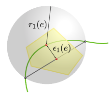
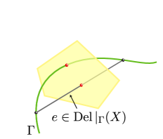
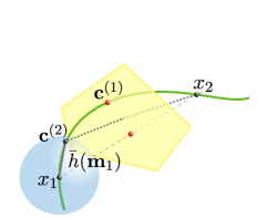
(i)	(ii)	(iii)

Figure 2: A restricted Delaunay 1-simplex $e\in\operatorname{Del}|_{\Gamma}\mathopen{}\mathclose{{}\left(X}\right)$ associated with a curve segment $\Gamma$, showing (i) the intersection of the associated Voronoi face $v_{f}\subseteq\operatorname{Vor}\mathopen{}\mathclose{{}\left(X}\right)$ and the curve network $\Gamma$, (ii) the associated Surface Delaunay Ball $\operatorname{SDB}(e)$, where $r_{1}(e)$ denotes the SDB radius and $\epsilon_{1}(e)$ the surface discretisation error, and (iii) the off-centre type refinement rule, showing the placement of a locally size-optimal point $\mathbf{c}^{(2)}$ about a frontal vertex $\mathbf{x}_{1}$.

3 A Restricted Delaunay-refinement Algorithm

An algorithm for the meshing of piecewise smooth complexes embedded in $\mathbb{R}^{3}$ is presented here, as an extension of previous work by the author in [1, 2, 3] and by various other authors, including: Rineau and Yvinec [20], Cheng, Dey and Shewchuk [4], Cheng, Dey and Levine [21], and Oudot, Rineaua and Yvinec [22]. This method is related to the CGALMESH algorithm – a classical restricted Delaunay-refinement approach available as part of the CGAL library [23], and summarised by Jamin, Alliez, Yvinec and Boissonnat in [14]. The algorithm presented here differs significantly in the methodology used for the recovery of 1-dimensional features. Specifically, in the current work, curve constraints are represented as an (unweighted) conforming restricted Delaunay sub-complex, as outlined in Section 2, and consistent with the techniques described by Rineau and Yvinec in [20]. The CGALMESH algorithm is instead based on a so-called protecting-balls strategy [4, 21], in which a static discretisation of the curve network $\Gamma$ is conducted as an initialisation step, with the resulting edge segments protected by a suitably-weighted Delaunay tessellation. Such a strategy preserves edge constraints throughout the subsequent surface- and volume-refinement iterations, though it does not guarantee that element quality thresholds are satisfied in the neighbourhood of such constraints. In some cases, this behaviour can lead to the creation of lower-quality elements adjacent to 1-dimensional features.

3.1 Preliminaries

As per Jamin et al. [14], the development of restricted Delaunay-refinement algorithms is geometry-agnostic, being independent of the specific definition of the underlying geometry inputs. It is required only that the framework support a set of so-called oracle predicates, used to compute: (i) the intersection of convex polygons (Voronoi faces) with the curve network $\Gamma$ (ii) the intersection of line segments (Voronoi edges) with the surface patches $\Sigma$, and (iii) the intersection of points (Voronoi vertices) with the enclosed volume $\Omega$. The Frontal-Delaunay algorithm presented in subsequent sections additionally requires the computation of intersections between the curves $\Gamma$ and surfaces $\Sigma$ with spheres and oriented disks. While a broad class of geometry descriptions are supported at the theoretical level, in this study, attention is restricted to the development of so-called re-meshing operations, in which the input geometries are specified in terms of discrete polylines and triangulated surfaces $\mathcal{P}$. This restriction is made to facilitate the construction of simple oracle predicates. Future work is intended to focus on the development of predicates for more general descriptions, including domains defined by implicit, parametric and analytic functions.

Following Jamin et al. [14], the Delaunay-refinement algorithm takes as input a volumetric domain $\Omega$, described by an enclosing (possibly non-manifold) surface $\Sigma\subseteq\mathbb{R}^{3}$, a network of curve segments $\Gamma\subseteq\mathbb{R}^{3}$, an upper bound on the allowable element radius-edge ratio $\bar{\rho}$, a mesh size function $\bar{h}\mathopen{}\mathclose{{}\left(\mathbf{x}}\right)$ defined at all points spanned by the domain, and an upper bound on the allowable surface discretisation error $\bar{\epsilon}(\mathbf{x})$. The algorithm returns a discretisation $\mathcal{T}|_{\Gamma}$ of the curve network $\Gamma$, a triangulation $\mathcal{T}|_{\Sigma}$ of the surface patches $\Sigma$, and a triangulation $\mathcal{T}|_{\Omega}$ of the enclosed volume $\Omega$. Here $\mathcal{T}|_{\Gamma}$, $\mathcal{T}|_{\Sigma}$ and $\mathcal{T}|_{\Omega}$ are restricted Delaunay sub-complexes, such that $\mathcal{T}|_{\Gamma}=\operatorname{Del}|_{\Gamma}\mathopen{}\mathclose{{}\left(X}\right)$, $\mathcal{T}|_{\Sigma}=\operatorname{Del}|_{\Sigma}\mathopen{}\mathclose{{}\left(X}\right)$ and $\mathcal{T}|_{\Omega}=\operatorname{Del}|_{\Omega}\mathopen{}\mathclose{{}\left(X}\right)$. Note that $\operatorname{Del}|_{\Gamma}\mathopen{}\mathclose{{}\left(X}\right)$ is an edge complex, $\operatorname{Del}|_{\Sigma}\mathopen{}\mathclose{{}\left(X}\right)$ is a triangular complex, and $\operatorname{Del}|_{\Omega}\mathopen{}\mathclose{{}\left(X}\right)$ and $\operatorname{Del}\mathopen{}\mathclose{{}\left(X}\right)$ are tetrahedral complexes. The Delaunay-refinement algorithm is summarised in Algorithm 3.1.

The Delaunay-refinement algorithm is designed to provide a number of geometrical and topological guarantees on the output mesh, specifically: (i) that all elements in the volumetric tessellation $\tau\in\mathcal{T}|_{\Omega}$ satisfy constraints on both the element shape and size, such that $\rho(\tau)\leq\bar{\rho}$, and $h(\tau)\leq\bar{h}\mathopen{}\mathclose{{}\left(\mathbf{x}_{\tau}}\right)$, (ii) that all elements in the embedded surface triangulation $f\in\mathcal{T}|_{\Sigma}$ are guaranteed to satisfy similar element shape and size constraints, in addition to an upper bound on the allowable surface discretisation error, such that $\epsilon(f)\leq\bar{\epsilon}(\mathbf{x}_{f})$, (iii) that the surface triangulation $\mathcal{T}|_{\Sigma}$ is topologically-consistent, ensuring that $\operatorname{Del}|_{\Sigma}\mathopen{}\mathclose{{}\left(X}\right)$ is uniformly 2-manifold in its interior, and is consistent with the input geometry at non-manifold features, (iv) that all elements in the embedded curve triangulation $e\in\mathcal{T}|_{\Gamma}$ are guaranteed to satisfy similar element size and surface error constraints, and (v) that the curve discretisation $\mathcal{T}|_{\Gamma}$ is also topologically-consistent, ensuring that $\operatorname{Del}|_{\Gamma}\mathopen{}\mathclose{{}\left(X}\right)$ is uniformly 1-manifold in its interior, and is consistent with the input geometry at non-manifold features. Making use of properties of the restricted Delaunay tessellation [17], it is known that the triangulations $\mathcal{T}|_{\Gamma}$, $\mathcal{T}|_{\Sigma}$ and $\mathcal{T}|_{\Omega}$ are good piecewise linear approximations to the input curves $\Gamma$, surfaces $\Sigma$ and volumes $\Omega$, provided that the magnitude of the mesh-size function $\bar{h}\mathopen{}\mathclose{{}\left(\mathbf{x}}\right)$ is sufficiently small. Under such conditions it is known that the triangulations $\mathcal{T}|_{\Gamma}$, $\mathcal{T}|_{\Sigma}$ and $\mathcal{T}|_{\Omega}$ are homeomorphic to the underlying curve, surface and volume definitions $\Gamma$, $\Sigma$ and $\Omega$, and that the geometrical properties of $\mathcal{T}|_{\Gamma}$, $\mathcal{T}|_{\Sigma}$ and $\mathcal{T}|_{\Omega}$ converge to the exact set of normals, curvatures, lengths, areas and volumes associated with the input geometry as $\bar{h}\mathopen{}\mathclose{{}\left(\mathbf{x}}\right)\rightarrow 0$.

3.2 Refinement Loop

Algorithm 3.1 Three-dimensional Restricted Delaunay-refinement

1:function DelaunayMesh($\Gamma,\Sigma,\Omega,\bar{\rho},\bar{\epsilon}(\mathbf{x}),\bar{h}\mathopen{}\mathclose{{}\left(\mathbf{x}}\right),\mathcal{T}|_{\Gamma},\mathcal{T}|_{\Sigma},\mathcal{T}|_{\Omega}$)

2:     Form an initial pointwise sampling $X$ such that $X$ is well-distributed on $\Gamma$ and $\Sigma$. Compute the Delaunay tessellation $\operatorname{Del}\mathopen{}\mathclose{{}\left(X}\right)$ and the restricted curve, surface and volume tessellations $\operatorname{Del}|_{\Gamma}\mathopen{}\mathclose{{}\left(X}\right)$, $\operatorname{Del}|_{\Sigma}\mathopen{}\mathclose{{}\left(X}\right)$ and $\operatorname{Del}|_{\Omega}\mathopen{}\mathclose{{}\left(X}\right)$.

3:     If some 1-simplex $e\in\operatorname{Del}|_{\Gamma}\mathopen{}\mathclose{{}\left(X}\right)$ violates BadSimplex1$(e)$, form the Steiner point $\mathbf{c}_{e}$ associated with $e$, insert $\mathbf{c}_{e}$ into $X$, update $\operatorname{Del}\mathopen{}\mathclose{{}\left(X}\right)$ and the restricted tessellations $\operatorname{Del}|_{\Gamma}\mathopen{}\mathclose{{}\left(X}\right)$, $\operatorname{Del}|_{\Sigma}\mathopen{}\mathclose{{}\left(X}\right)$ and $\operatorname{Del}|_{\Omega}\mathopen{}\mathclose{{}\left(X}\right)$ and go to step 3.

4:     For all vertices $p\in\operatorname{Del}|_{\Gamma}\mathopen{}\mathclose{{}\left(X}\right)$ compute $\mathbf{c}_{p}\leftarrow$TopoDisk1$(p)$. If $\mathbf{c}_{p}$ is non-null, insert $\mathbf{c}_{p}$ into $X$, update $\operatorname{Del}\mathopen{}\mathclose{{}\left(X}\right)$ and the restricted tessellations $\operatorname{Del}|_{\Gamma}\mathopen{}\mathclose{{}\left(X}\right)$, $\operatorname{Del}|_{\Sigma}\mathopen{}\mathclose{{}\left(X}\right)$ and $\operatorname{Del}|_{\Omega}\mathopen{}\mathclose{{}\left(X}\right)$ and go to step 3.

5:     If some 2-simplex $f\in\operatorname{Del}|_{\Sigma}\mathopen{}\mathclose{{}\left(X}\right)$ violates BadSimplex2$(f)$, form the Steiner point $\mathbf{c}_{f}$ associated with $f$: 1. If the point $\mathbf{c}_{f}$ lies within a surface ball $B(\mathbf{c}_{e},r)$ associated with some 1-face $e\in\operatorname{Del}|_{\Gamma}\mathopen{}\mathclose{{}\left(X}\right)$, insert $\mathbf{c}_{e}$ into $X$ instead, update $\operatorname{Del}\mathopen{}\mathclose{{}\left(X}\right)$ and the restricted tessellations $\operatorname{Del}|_{\Gamma}\mathopen{}\mathclose{{}\left(X}\right)$, $\operatorname{Del}|_{\Sigma}\mathopen{}\mathclose{{}\left(X}\right)$ and $\operatorname{Del}|_{\Omega}\mathopen{}\mathclose{{}\left(X}\right)$ and go to step 3. 2. Insert $\mathbf{c}_{f}$ into $X$. If $\mathbf{c}_{f}$ changes the topology of $\operatorname{Del}|_{\Gamma}\mathopen{}\mathclose{{}\left(X}\right)$, find the largest adjacent surface ball $B(\mathbf{c}_{e},r)$, delete $\mathbf{c}_{f}$ from $X$ and insert $\mathbf{c}_{e}$ into $X$. update $\operatorname{Del}\mathopen{}\mathclose{{}\left(X}\right)$ and the restricted tessellations $\operatorname{Del}|_{\Gamma}\mathopen{}\mathclose{{}\left(X}\right)$, $\operatorname{Del}|_{\Sigma}\mathopen{}\mathclose{{}\left(X}\right)$ and $\operatorname{Del}|_{\Omega}\mathopen{}\mathclose{{}\left(X}\right)$ and go to step 3. 3. Go to step 5.

6:     For all vertices $p\in\operatorname{Del}|_{\Sigma}\mathopen{}\mathclose{{}\left(X}\right)$ compute $\mathbf{c}_{p}\leftarrow$TopoDisk2$(p)$. If $\mathbf{c}_{p}$ is non-null, insert $\mathbf{c}_{p}$ into $X$, update $\operatorname{Del}\mathopen{}\mathclose{{}\left(X}\right)$ and the restricted tessellations $\operatorname{Del}|_{\Gamma}\mathopen{}\mathclose{{}\left(X}\right)$, $\operatorname{Del}|_{\Sigma}\mathopen{}\mathclose{{}\left(X}\right)$ and $\operatorname{Del}|_{\Omega}\mathopen{}\mathclose{{}\left(X}\right)$ and go to step 3.

7:     If some 3-simplex $\tau\in\operatorname{Del}|_{\Omega}\mathopen{}\mathclose{{}\left(X}\right)$ violates BadSimplex3$(f\tau)$, form the Steiner point $\mathbf{c}_{\tau}$ associated with $\tau$: 1. If the point $\mathbf{c}_{\tau}$ lies within a surface ball $B(\mathbf{c}_{e},r)$ associated with some 1-face $e\in\operatorname{Del}|_{\Gamma}\mathopen{}\mathclose{{}\left(X}\right)$, insert $\mathbf{c}_{e}$ into $X$ instead, update $\operatorname{Del}\mathopen{}\mathclose{{}\left(X}\right)$ and the restricted tessellations $\operatorname{Del}|_{\Gamma}\mathopen{}\mathclose{{}\left(X}\right)$, $\operatorname{Del}|_{\Sigma}\mathopen{}\mathclose{{}\left(X}\right)$ and $\operatorname{Del}|_{\Omega}\mathopen{}\mathclose{{}\left(X}\right)$ and go to step 3. 2. If the point $\mathbf{c}_{\tau}$ lies within a surface ball $B(\mathbf{c}_{f},r)$ associated with some 2-face $f\in\operatorname{Del}|_{\Sigma}\mathopen{}\mathclose{{}\left(X}\right)$, insert $\mathbf{c}_{f}$ into $X$ instead, update $\operatorname{Del}\mathopen{}\mathclose{{}\left(X}\right)$ and the restricted tessellations $\operatorname{Del}|_{\Gamma}\mathopen{}\mathclose{{}\left(X}\right)$, $\operatorname{Del}|_{\Sigma}\mathopen{}\mathclose{{}\left(X}\right)$ and $\operatorname{Del}|_{\Omega}\mathopen{}\mathclose{{}\left(X}\right)$ and go to step 3. 3. Insert $\mathbf{c}_{\tau}$ into $X$. If $\mathbf{c}_{\tau}$ changes the topology of $\operatorname{Del}|_{\Gamma}\mathopen{}\mathclose{{}\left(X}\right)$, find the largest adjacent surface ball $B(\mathbf{c}_{e},r)$, delete $\mathbf{c}_{\tau}$ from $X$ and insert $\mathbf{c}_{e}$ into $X$. update $\operatorname{Del}\mathopen{}\mathclose{{}\left(X}\right)$ and the restricted tessellations $\operatorname{Del}|_{\Gamma}\mathopen{}\mathclose{{}\left(X}\right)$, $\operatorname{Del}|_{\Sigma}\mathopen{}\mathclose{{}\left(X}\right)$ and $\operatorname{Del}|_{\Omega}\mathopen{}\mathclose{{}\left(X}\right)$ and go to step 3. 4. Insert $\mathbf{c}_{\tau}$ into $X$. If $\mathbf{c}_{\tau}$ changes the topology of $\operatorname{Del}|_{\Sigma}\mathopen{}\mathclose{{}\left(X}\right)$, find the largest adjacent surface ball $B(\mathbf{c}_{f},r)$, delete $\mathbf{c}_{\tau}$ from $X$ and insert $\mathbf{c}_{f}$ into $X$. update $\operatorname{Del}\mathopen{}\mathclose{{}\left(X}\right)$ and the restricted tessellations $\operatorname{Del}|_{\Gamma}\mathopen{}\mathclose{{}\left(X}\right)$, $\operatorname{Del}|_{\Sigma}\mathopen{}\mathclose{{}\left(X}\right)$ and $\operatorname{Del}|_{\Omega}\mathopen{}\mathclose{{}\left(X}\right)$ and go to step 3. 5. Go to step 7.

8:     Return the final restricted Delaunay curve, surface and volume tessellations $\operatorname{Del}|_{\Gamma}\mathopen{}\mathclose{{}\left(X}\right)$, $\operatorname{Del}|_{\Sigma}\mathopen{}\mathclose{{}\left(X}\right)$ and $\operatorname{Del}|_{\Omega}\mathopen{}\mathclose{{}\left(X}\right)$.

9:end function

The Delaunay-refinement algorithm begins by pre-processing the input geometry – seeking to identify any sharp-features inscribed on the input curve and surface collections. These 0- and 1-dimensional features can be induced by both geometrical and topological constraints, including: (i) features that form sharp creases or corners in $\Gamma$ and/or $\Sigma$, and (ii) features at the apex of non-manifold topological connections. After pre-processing, an initial point-wise sampling of the input curve and surface segments $\Gamma$ and $\Sigma$ is created. Exploiting the discrete representations available, the initial sampling is obtained in this study as a well-distributed subset of the existing vertices $Y\in\mathcal{P}$, where $\mathcal{P}$ is the polyhedral representation of the curve and surface segments $\Gamma$ and $\Sigma$. In the next step, the initial triangulation objects are formed. In this work, the full-dimensional Delaunay tessellation, $\operatorname{Del}\mathopen{}\mathclose{{}\left(X}\right)$, is built using an incremental Delaunay triangulation algorithm, based on the Bowyer-Watson technique [24]. The restricted curve, surface and volumetric triangulations, $\operatorname{Del}|_{\Gamma}\mathopen{}\mathclose{{}\left(X}\right)$, $\operatorname{Del}|_{\Sigma}\mathopen{}\mathclose{{}\left(X}\right)$ and $\operatorname{Del}|_{\Omega}\mathopen{}\mathclose{{}\left(X}\right)$, are derived from the topology of $\operatorname{Del}\mathopen{}\mathclose{{}\left(X}\right)$ by explicitly testing for intersections between the faces of the associated Voronoi complex $\operatorname{Vor}\mathopen{}\mathclose{{}\left(X}\right)$ and the input curve and surface segments $\Gamma$ and $\Sigma$. These queries are computed efficiently by storing the polyhedral geometry $\mathcal{P}$ in an aabb-tree [3, 25].

Algorithm 3.2 Topological Disks & Termination Criteria

1:function TopoDisk1($p$)

2:     Find the set of 1-simplexes $E_{p}\in\operatorname{Del}|_{\Gamma}\mathopen{}\mathclose{{}\left(X}\right)$ adjacent to the vertex $p$.

3:     If $E_{p}$ is either empty or a valid topological $1$-disk, return NULL. Otherwise, find the 1-simplex $e\in E_{p}$ that maximises the size of the associated surface Delaunay ball $B(\mathbf{c}_{e},r)$ and return $\mathbf{c}_{e}$.

4:end function

1:function TopoDisk2($p$)

2:     Find the set of 2-simplexes $F_{p}\in\operatorname{Del}|_{\Sigma}\mathopen{}\mathclose{{}\left(X}\right)$ adjacent to the vertex $p$.

3:     If $F_{p}$ is either empty or a valid topological $2$-disk, return NULL. Otherwise, find the 2-simplex $f\in F_{p}$ that maximises the size of the associated surface Delaunay ball $B(\mathbf{c}_{f},r)$ and return $\mathbf{c}_{f}$.

4:end function

  1:function BadSimplex1($e$) 2:     if $(\epsilon_{1}(e)>\bar{\epsilon}(\mathbf{x}_{e}))$ return TRUE if $(h\,(e)>\bar{h}(\mathbf{x}_{e}))$ return TRUE else, return FALSE 3:end function 1:function BadSimplex2($f$) 2:     if $(\epsilon_{2}(f)>\bar{\epsilon}(\mathbf{x}_{f}))$ return TRUE if $(h\,(f)>\bar{h}(\mathbf{x}_{f}))$ return TRUE if $(\rho_{2}(f)>\bar{\rho})$ return TRUE else, return FALSE 3:end function 1:function BadSimplex3($\tau$) 2:     if $(h(\tau)>\bar{h}(\mathbf{x}_{\tau}))$ return TRUE if $(\rho_{3}(\tau)>\bar{\rho})$ return TRUE else, return FALSE 3:end function

The main loop of the algorithm proceeds to incrementally refine any restricted 1-, 2- or 3-simplexes found to be in violation of one or more geometrical or topological constraints. Specifically, in steps 3, 5 and 7, any simplexes $e\in\operatorname{Del}|_{\Gamma}\mathopen{}\mathclose{{}\left(X}\right)$, $f\in\operatorname{Del}|_{\Sigma}\mathopen{}\mathclose{{}\left(X}\right)$ or $\tau\in\operatorname{Del}|_{\Omega}\mathopen{}\mathclose{{}\left(X}\right)$ found to violate a set of local topological, radius-edge, mesh-size or surface-error constraints are refined – through the introduction of a new Steiner point $\mathbf{c}_{e}$, $\mathbf{c}_{f}$ or $\mathbf{c}_{\tau}$ located at the centre of the associated surface balls $B(\mathbf{c}_{e},r)$, $B(\mathbf{c}_{f},r)$ or circumscribing ball $B(\mathbf{c}_{\tau},r)$. Importantly, refinement proceeds in a hierarchical manner, with the insertion of $\mathbf{c}_{f}$ and $\mathbf{c}_{\tau}$ dependent on several additional constraints designed to preserve the consistency of the lower dimensional tessellations $\operatorname{Del}|_{\Gamma}\mathopen{}\mathclose{{}\left(X}\right)$ and $\operatorname{Del}|_{\Sigma}\mathopen{}\mathclose{{}\left(X}\right)$. Specifically, in steps 5a–5b and 7a–7d a set of encroachment conditions are enforced, with refinement cascading onto lower-dimensional simplexes if a set of geometrical or topological constraints are violated. In steps 5a and 7a, 7c, if $\mathbf{c}_{f}$ or $\mathbf{c}_{\tau}$ are found to lie within the surface balls $B(\mathbf{c}_{e},r)$ or $B(\mathbf{c}_{f},r)$ of an existing curve or surface facet, that facet is instead refined, through the insertion of a Steiner vertex located at the centre of the associated surface ball $\mathbf{c}_{e}$ or $\mathbf{c}_{f}$. This process can be seen simply as an extension of the standard edge-encroachment scheme used in Ruppert’s two-dimensional refinement algorithm. In steps 5b and 7b, 7d, if the insertion of $\mathbf{c}_{f}$ or $\mathbf{c}_{\tau}$ is found to modify the restricted triangulations $\operatorname{Del}|_{\Gamma}\mathopen{}\mathclose{{}\left(X}\right)$ or $\operatorname{Del}|_{\Sigma}\mathopen{}\mathclose{{}\left(X}\right)$, the insertion is deferred onto an adjacent curve or surface facet. Specifically, the point $\mathbf{c}_{f}$ or $\mathbf{c}_{\tau}$ is deleted from $\operatorname{Del}\mathopen{}\mathclose{{}\left(X}\right)$ and a new Steiner vertex $\mathbf{c}_{e}$ or $\mathbf{c}_{f}$, corresponding to the centre of the largest adjacent surface ball, is inserted instead. This process ensures that the consistency of the curve and surface tessellations $\operatorname{Del}|_{\Gamma}\mathopen{}\mathclose{{}\left(X}\right)$ and $\operatorname{Del}|_{\Sigma}\mathopen{}\mathclose{{}\left(X}\right)$ is preserved by subsequent refinement operations.

In additional to this element-by-element refinement, the topological consistency of the restricted curve and surface tessellations is also enforced in aggregate, by ensuring that the set of 1- and 2-simplexes $E_{p}\in\operatorname{Del}|_{\Gamma}\mathopen{}\mathclose{{}\left(X}\right)$ and $F_{p}\in\operatorname{Del}|_{\Sigma}\mathopen{}\mathclose{{}\left(X}\right)$ adjacent to each vertex $p\in\operatorname{Del}\mathopen{}\mathclose{{}\left(X}\right)$ form locally 1- and 2-manifold features, known as topological 1- and 2-disks. Vertices adjacent to non-manifold connections trigger additional refinement operations, with the centres $\mathbf{c}_{e}$ and $\mathbf{c}_{f}$ of the largest adjacent surface balls $B(\mathbf{c}_{e},r)$ and $B(\mathbf{c}_{f},r)$ associated with the simplexes $e\in E_{p}$ and $f\in F_{p}$ inserted as new Steiner vertices until local topological consistency is recovered. Specifically, a cascade of new Steiner vertices are inserted until the topology of $\operatorname{Del}|_{\Gamma}\mathopen{}\mathclose{{}\left(X}\right)$ and $\operatorname{Del}|_{\Sigma}\mathopen{}\mathclose{{}\left(X}\right)$, sampled at all points $p\in\operatorname{Del}\mathopen{}\mathclose{{}\left(X}\right)$, is equivalent to that of the input curve and surface complexes $\Gamma$ and $\Sigma$.

The refinement process continues until all radius-edge, mesh-size, surface-error and topological constraints are satisfied for all simplexes $e\in\operatorname{Del}|_{\Gamma}\mathopen{}\mathclose{{}\left(X}\right)$, $f\in\operatorname{Del}|_{\Sigma}\mathopen{}\mathclose{{}\left(X}\right)$ and $\tau\in\operatorname{Del}|_{\Omega}\mathopen{}\mathclose{{}\left(X}\right)$. The refinement process is priority scheduled, with triangles $f\in\operatorname{Del}|_{\Sigma}\mathopen{}\mathclose{{}\left(X}\right)$ and tetrahedrons $\tau\in\operatorname{Del}|_{\Omega}\mathopen{}\mathclose{{}\left(X}\right)$ ordered according to their radius-edge ratios $\rho\mathopen{}\mathclose{{}\left(f}\right)$ and $\rho\mathopen{}\mathclose{{}\left(\tau}\right)$, ensuring that the element with the worst ratio is refined at each iteration. Segments in $\operatorname{Del}|_{\Gamma}\mathopen{}\mathclose{{}\left(X}\right)$ are ordered according to the size of their surface balls. Mesh-size constraints are applied with respect to the size of the circumscribing balls associated with each element. Specifically, the mean element sizes $h(e)=2\,r_{e}$, $h(f)=\sqrt{3}\,r_{f}$ and $h(\tau)=\sqrt{\nicefrac{{8}}{{3}}}\,r_{\tau}$ are used throughout, where $h(e)$, $h(f)$ and $h(\tau)$ denote the size associated with segments, triangles and tetrahedrons respectively. The scalar coefficients represent mappings between circumball radii and edge length for equilateral elements. In this study, mesh-size constraints are implemented as $h(e)\leq\alpha\bar{h}(\mathbf{x}_{e})$, $h(f)\leq\alpha\bar{h}(\mathbf{x}_{f})$ and $h(\tau)\leq\alpha\bar{h}(\mathbf{x}_{\tau})$, where $\alpha=\nicefrac{{4}}{{3}}$ is a constant factor designed to ensure that mean element size does not, on average, undershoot the target size. The local mesh-size values $\bar{h}(\mathbf{x}_{e})$, $\bar{h}(\mathbf{x}_{f})$ and $\bar{h}(\mathbf{x}_{\tau})$ are evaluated at the centres of the associated circumballs.

4 Feature Conforming Off-centre Steiner Points

Frontal-Delaunay algorithms are a hybridisation of advancing-front and Delaunay-refinement techniques, in which a Delaunay triangulation is used to define the topology of a mesh while Steiner vertices are inserted consistent with advancing-front type methodologies. In practice, such techniques have been observed to produce very high-quality meshes, inheriting the smooth, semi-structured vertex placement of pure advancing-front methods and the optimal mesh topology and robustness of Delaunay-based approaches. Such techniques have been employed in a number of studies, including, for example [26, 27, 28, 29, 30, 31, 32] and previous work by the author [1, 2, 3].

4.1 Point-placement Strategy (Edge Segments)

The off-centre strategy used to refine curve segments is based on methods previously developed by the author [1, 2, 3] for surface and volume refinement. Two candidate Steiner vertices are considered. Type I vertices, $\mathbf{c}^{(1)}$, are equivalent to conventional element circumcentres (positioned at the centre of the associated surface balls), and are used to preserve global convergence. Type II vertices, $\mathbf{c}^{(2)}$, are so-called size-optimal points, and are designed to satisfy mesh-size constraints in a locally optimal fashion. Given a refinable 1-simplex $e\in\operatorname{Del}|_{\Gamma}\mathopen{}\mathclose{{}\left(X}\right)$, the Type II vertex $\mathbf{c}^{(2)}$ is positioned at an intersection of the curve network $\Gamma$, and a sphere $S_{\sigma}$ of radius $\bar{h}_{\sigma}$, centred on a vertex $\mathbf{x}_{1}\in e$. The vertex $\mathbf{c}^{(2)}$ is positioned such that it forms an edge candidate $\sigma$ about the frontal vertex $\mathbf{x}_{1}$, such that its size $h\mathopen{}\mathclose{{}\left(\sigma}\right)$ satisfies $\bar{h}(\mathbf{x})$. Specifically, the length of $\sigma$ is computed from local mesh-size information, such that:

$${\bar{h}_{\sigma}}=\tfrac{1}{2}\mathopen{}\mathclose{{}\left({\bar{h}(\mathbf{x}_{1})}+{\bar{h}(\mathbf{c}^{(2)})}}\right).$$ (1)

For non-uniform $\bar{h}\mathopen{}\mathclose{{}\left(\mathbf{x}}\right)$, this expression is weakly non-linear, and an iterative procedure is used to obtain an approximate solution. In the case of multiple intersections between the curve network $\Gamma$ and the sphere $S_{\sigma}$, the point $\mathbf{c}_{j}^{(2)}$ that minimises the angle to the frontal vector $\mathbf{v}$ is chosen, where $\mathbf{v}$ is oriented from the frontal vertex $\mathbf{x}_{1}$ to the centre of the surface ball $B(\mathbf{c}_{e},r)$. See Figure 2(iii) for additional illustration.

4.2 Point-placement Strategy (Triangles & Tetrahedrons)

Similar techniques are used to refine triangles and tetrahedrons, with two candidate Steiner vertices used to balance local optimality and global convergence guarantees. These methods are presented by the author in detail in [1, 2].

4.3 Point-placement Strategy (Off-centre Selection)

Given the sets of Type I and Type II off-centres $\mathbf{c}_{e,\,f,\,\tau}^{(1)}$ and $\mathbf{c}_{e,\,f,\,\tau}^{(2)}$ available for curve, surface and volume elements, respectively, the positions of the associated refinement points $\mathbf{c}_{e}$, $\mathbf{c}_{f}$ and $\mathbf{c}_{\tau}$ are calculated. These points are selected to satisfy the limiting local constraints, setting

$$\mathbf{c}_{e}=\mathopen{}\mathclose{{}\left\{\begin{array}[]{ll}\mathbf{c}^{(2)}_{e},&\text{ if }\big{(}d^{(2)}_{e}\leq d^{(1)}_{e}\big{)}\\[4.30554pt] \mathbf{c}^{(1)}_{e},&\text{ otherwise}\end{array}}\right.\quad\text{and}\quad\mathbf{c}_{f,\,\tau}=\mathopen{}\mathclose{{}\left\{\begin{array}[]{ll}\mathbf{c}^{(2)}_{f,\,\tau},&\text{ if }\big{(}d^{(2)}_{f,\,\tau}\leq d^{(1)}_{f,\,\tau}\big{)}\text{ and }\big{(}d^{(2)}_{f,\,\tau}\geq r_{0}\big{)}\\[4.30554pt] \mathbf{c}^{(1)}_{f,\,\tau},&\text{ otherwise }\end{array}}\right.\quad$$ (2)

where $d^{(i)}=\|\mathbf{c}^{(i)}-\mathbf{c}_{0}\|$ are distances from the centre of the frontal facet to the Type I and Type II points, respectively and $r_{0}$ is the radius of the diametric ball associated with the frontal face or vertex. This cascading selection criteria ensures that refinement scheme smoothly degenerates to that of a conventional circumcentre-based Delaunay-refinement strategy in limiting cases, while using locally optimal points where possible. Specifically, these constraints guarantee that the refinement points for curve, surface and volume elements lie within a local safe region on the Voronoi complex – being positioned on an adjacent Voronoi sub-face and bound between the circumcentre of the element itself and the diametric ball of the associated frontal entity. See previous work by the author [1, 2, 3] for additional details.

4.4 Refinement Order

In addition to off-centre point-placement rules, the Frontal-Delaunay algorithm also relies on changes to the order in which elements are refined. To better mimic the behaviour of advancing-front type methods, elements are refined only if they are adjacent to existing frontal entities. In the case of curve facets $e\in\operatorname{Del}|_{\Gamma}\mathopen{}\mathclose{{}\left(X}\right)$, the frontal vertex $\mathbf{x}_{i}\in e$ must be shared by at least one adjacent facet $e_{j}\in\operatorname{Del}|_{\Gamma}\mathopen{}\mathclose{{}\left(X}\right)$ that is converged – satisfying its associated topological and geometrical constraints. In the case of surface triangles $f\in\operatorname{Del}|_{\Sigma}\mathopen{}\mathclose{{}\left(X}\right)$ and interior tetrahedrons $\tau\in\operatorname{Del}|_{\Omega}\mathopen{}\mathclose{{}\left(X}\right)$, the frontal facet $e_{0}\in f$, $f_{0}\in\tau$ must either be a converged simplex $e_{j}\in\operatorname{Del}|_{\Gamma}\mathopen{}\mathclose{{}\left(X}\right)$, $f_{j}\in\operatorname{Del}|_{\Sigma}\mathopen{}\mathclose{{}\left(X}\right)$ or be shared by an adjacent simplex $f_{j}\in\operatorname{Del}|_{\Sigma}\mathopen{}\mathclose{{}\left(X}\right)$, $\tau_{j}\in\operatorname{Del}|_{\Omega}\mathopen{}\mathclose{{}\left(X}\right)$ satisfying its associated constraints. In rare cases where no frontal simplex can be found (such as in the initial stages of refinement, where all faces in $\operatorname{Del}\mathopen{}\mathclose{{}\left(X}\right)$ are still very coarse with respect to $\bar{h}(\mathbf{x})$), standard circumcentre-based refinement is used as a fall-back, ensuring convergence. Use of this type of implicit frontal boundary between converged and un-converged elements is a common feature of Frontal-Delaunay algorithms, with similar approaches used by, for example, [27, 28, 29, 30].

4.5 Termination, Convergence & Correctness

The termination and convergence of the Frontal-Delaunay refinement algorithm can be analysed by considering the behaviour of the point-placement rules described previously. For the sake of brevity, a full analysis is not included here, instead a theoretical ‘sketch’ is presented. Firstly, it is important to note that the off-centre vertices selected by the algorithm reduce to standard element circumcentres in limiting cases:

Remark 4.1.

Let $\bar{h}(\boldsymbol{x})\geq\bar{h}_{0},\bar{h}_{0}\in\mathbb{R}^{+}$ be a positive mesh-size function and $\operatorname{Del}|_{\Gamma}\mathopen{}\mathclose{{}\left(X_{k}}\right)$, $\operatorname{Del}|_{\Sigma}\mathopen{}\mathclose{{}\left(X_{k}}\right)$ and $\operatorname{Del}|_{\Omega}\mathopen{}\mathclose{{}\left(X_{k}}\right)$ be the restricted triangulation objects after $k$ refinement steps. Given a refinable simplex $e\in\operatorname{Del}|_{\Gamma}\mathopen{}\mathclose{{}\left(X_{k}}\right)$, $f\in\operatorname{Del}|_{\Sigma}\mathopen{}\mathclose{{}\left(X_{k}}\right)$ or $\tau\in\operatorname{Del}|_{\Omega}\mathopen{}\mathclose{{}\left(X_{k}}\right)$, use of the Type II point-placement scheme is ‘declined’ if $r\leq\bar{h}_{\sigma}$, where $r$ is the radius of the circumscribing ball $B(\boldsymbol{x}_{e,f,\tau},r)$ and $\bar{h}_{\sigma}$ is the local element ‘length’ computed by the Type II point-placement rule.

This behaviour is a consequence of the off-centre selection rules (2), requiring that the refinement point for any 1-, 2- or 3-simplex is the off-centre candidate $\mathbf{c}^{(1)}$ or $\mathbf{c}^{(2)}$ that minimises the distance to the centre of the diametric ball $\operatorname{B}(\mathbf{c}_{0},r_{0})$ associated with the frontal face or vertex. Noting that $\mathbf{c}^{(1)}$ and $\mathbf{c}^{(2)}$ are located on an adjacent segment of $\operatorname{Vor}\mathopen{}\mathclose{{}\left(X}\right)$, it is clear that $\|\mathbf{c}^{(2)}-\mathbf{c}_{0}\|\leq\|\mathbf{c}^{(1)}-\mathbf{c}_{0}\|$ only if $r\geq\bar{h}_{\sigma}$.

Considering that standard, circumcentre-type insertion rules are recovered when elements become sufficiently small, the overall termination of the algorithm is equivalent to that of a conventional circumcentre-based scheme. In [20], Rineau and Yvinec analyse such an approach, and have shown that, under the assumption of non-acute input, termination is guaranteed provided that:

$$\bar{\rho}_{f}\geq\Big{(}\!\sqrt{2}+2\Big{)}\nu_{0}\quad\text{and}\quad\bar{\rho}_{\tau}\geq\Big{(}\!\sqrt{2}+2\Big{)}\nu_{0}\Big{(}\nu_{0}+2\Big{)}$$ (3)

where $\nu_{0}=\nicefrac{{2\mu_{0}}}{{\gamma_{0}}}$ is a mesh-size ratio, given $\mu_{0}$ as the maximum of $\bar{h}(\mathbf{x})$ over the surface patches $\Sigma$ and $\gamma_{0}$ as the minimum of $\bar{h}(\mathbf{x})$ over the volumes $\Omega$. Typically, the algorithm is found to outperform these bounds in practice.

Finite termination leads directly to a number of useful auxiliary guarantees on both the nature and quality of the output tessellation. Adopting the conventional terminology, meshes generated using the Delaunay-refinement and Frontal-Delaunay refinement algorithms presented here can be considered to be provably-good:

Remark 4.2.

If the meshing algorithm terminates after $k$ steps, the restricted curve, surface and volume sub-complexes $\operatorname{Del}|_{\Gamma}\mathopen{}\mathclose{{}\left(X_{k}}\right)$, $\operatorname{Del}|_{\Sigma}\mathopen{}\mathclose{{}\left(X_{k}}\right)$ and $\operatorname{Del}|_{\Omega}\mathopen{}\mathclose{{}\left(X_{k}}\right)$ satisfy the following properties:

(A) size & shape-quality: The size and shape of elements in the output mesh satisfy several constraints. Specifically, all elements $e\in\operatorname{Del}|_{\Gamma}\mathopen{}\mathclose{{}\left(X_{k}}\right)$, $f\in\operatorname{Del}|_{\Sigma}\mathopen{}\mathclose{{}\left(X_{k}}\right)$ and $\tau\in\operatorname{Del}|_{\Omega}\mathopen{}\mathclose{{}\left(X_{k}}\right)$ contain bounded radius-edge ratios and circumball sizes, such that: (i) $\rho(f)\leq\bar{\rho}_{f}$ and $\rho(\tau)\leq\bar{\rho}_{\tau}$, and (ii) $h(e)\leq\alpha\bar{h}(\mathbf{x}_{e})$, $h(f)\leq\alpha\bar{h}(\mathbf{x}_{f})$ and $h(\tau)\leq\alpha\bar{h}(\mathbf{x}_{\tau})$, where $\alpha=\nicefrac{{4}}{{3}}$ and $h(e)=2\,r_{e}$, $h(f)=\sqrt{3}\,r_{f}$ and $h(\tau)=\sqrt{\nicefrac{{8}}{{3}}}\,r_{\tau}$ are scaled circumball radii.

(B) approximation error: The surface discretisation error associated with the output mesh is bounded by a one-sided threshold on the Hausdorff distance. Specifically, all elements $e\in\operatorname{Del}|_{\Gamma}\mathopen{}\mathclose{{}\left(X_{k}}\right)$ and $f\in\operatorname{Del}|_{\Sigma}\mathopen{}\mathclose{{}\left(X_{k}}\right)$, contain bounded surface error measures, such that $\epsilon(e)\leq\bar{\epsilon}(\mathbf{x}_{e})$ and $\epsilon(f)\leq\bar{\epsilon}(\mathbf{x}_{f})$.

(C) topological consistency: The output mesh is consistent with the topology of the input geometry, consisting of curve and surface tessellations that are locally 1- and 2-manifold in their interiors, and share the degree of the input features at their boundaries.

The algorithm maintains a queue of bad elements, $e\in\operatorname{Del}|_{\Gamma}\mathopen{}\mathclose{{}\left(X_{k}}\right)$, $f\in\operatorname{Del}|_{\Sigma}\mathopen{}\mathclose{{}\left(X_{k}}\right)$, $\tau\in\operatorname{Del}|_{\Omega}\mathopen{}\mathclose{{}\left(X_{k}}\right)$ and vertices $p\in\operatorname{Del}\mathopen{}\mathclose{{}\left(X}\right)$, in violation of one or more local constraints. Given that termination of the algorithm is guaranteed, it is clear that the refinement queues must become empty, and that the output mesh satisfies the requisite geometrical and topological constraints as a result.

The development of a full theoretical model of termination, convergence and correctness for the new algorithms presented here is the subject of a forthcoming publication.

5 Protecting Sharp Angles Between Curves

Like all Delaunay-refinement type methods, the restricted Delaunay-refinement and Frontal-Delaunay algorithms presented here suffer from issues of non-convergence when the input domain contains sharply acute features. In such cases, a special-case pre-processing phase is required to identify and to protect such features. In this study, a technique to protect sharp angles subtended by 1-dimensional features is described. The development of a generalised procedure for sharp features between 2-dimensional surface patches is deferred for future investigation. Specifically, a process modelled on the two-dimensional corner-lopping procedure of Pav and Walkington [33] and the three-dimensional protective-collar techniques of Rand and Walkington [34, 35] is adopted, in which a small subset of the domain, adjacent to any sufficiently sharp features, is pre-processed and quarantined from subsequent refinement operations. Note that this collar-based approach is fundamentally different from the standard protecting-ball type techniques utilised in other (statically weighted) restricted Delaunay-refinement algorithms [21, 4, 14]. Specifically, in the current work, a standard (unweighted) Delaunay triangulation is forced to conform to sharp-features in the input geometry via a judicious arrangement of local Steiner vertices.

Given a sharply acute internal angle $\mathcal{A}_{ij}\leq\nicefrac{{\pi}}{{3}}$ formed by any pair of segments $i,j$ in the curve network $\Gamma$, the protection process proceeds in a staged fashion: (i) a vertex $\mathbf{x}_{\mathcal{A}}$ is introduced at the apex of the sharp angle $\mathcal{A}_{ij}$, (ii) two new vertices $\mathbf{x}_{i},\mathbf{x}_{j}$ are positioned along the incident curve segments $i,j\in\Gamma$, such that an isosceles triangle candidate $[\mathbf{x}_{\mathcal{A}},\mathbf{x}_{i},\mathbf{x}_{j}]$ is formed. Specifically, the points $\mathbf{x}_{i},\mathbf{x}_{j}$ are positioned at the intersection of a ball of radius $r_{\mathcal{A}}$, centred at $\mathbf{x}_{\mathcal{A}}$, and the curve network $\Gamma$. Ideally, the radius $r_{\mathcal{A}}$ should be chosen to reflect the local-feature-size at the apex of the sharp angle $\operatorname{lfs}(\mathbf{x}_{\mathcal{A}})$. In practice, such a quantity is hard to compute reliably, and the radius $r_{\mathcal{A}}$ is computed using an iterative procedure in the present work instead. In this process, the local mesh-size $\bar{h}(\mathbf{x}_{\mathcal{A}})$ is used as an initial guess for the radius $r_{\mathcal{A}}$. The radius is then iteratively reduced until: (i) there exist exactly two intersections between the ball $\operatorname{B}(\mathbf{x}_{\mathcal{A}},r_{\mathcal{A}})$ and the curve network $\Gamma$, and (ii) the ball $\operatorname{B}(\mathbf{x}_{\mathcal{A}},\beta r_{\mathcal{A}})$ is empty of intersections with other balls centred on protected features in $\Gamma$. Here, the scalar $\beta\geq 1$ is a spacing-factor, ensuring that adjacent balls are sufficiently well separated. In this study $\beta=\nicefrac{{3}}{{2}}$ is used. The protection procedure presented here is similar to the SplitBall operator described in [33] for two-dimensional piecewise smooth domains.

Noting that such a set of protecting balls is disjoint, and that the candidate vertices describe sets of well-centred isosceles triangles, it is clear that the Delaunay tessellation $\operatorname{Del}\mathopen{}\mathclose{{}\left(X}\right)$ contains both the protected edge segments $[\mathbf{x}_{\mathcal{A}},\mathbf{x}_{i}]$ and $[\mathbf{x}_{\mathcal{A}},\mathbf{x}_{j}]$, in addition to the triangles $[\mathbf{x}_{\mathcal{A}},\mathbf{x}_{i},\mathbf{x}_{j}]$, thus constituting a conforming Delaunay triangulation of the sharp features in $\Gamma$. Clearly, these protected elements are also automatically included in the restricted sub-complexes $\operatorname{Del}|_{\Gamma}\mathopen{}\mathclose{{}\left(X}\right)$ and $\operatorname{Del}|_{\Sigma}\mathopen{}\mathclose{{}\left(X}\right)$. The main loop of the Delaunay-refinement algorithm is modified to ensure that these protected elements are preserved throughout the refinement passes. In this study, a simple topological constraint is enforced: any new Steiner vertex found to delete a protected edge $e_{\mathcal{A}}\in\operatorname{Del}|_{\Gamma}\mathopen{}\mathclose{{}\left(X}\right)$ is rejected. In practice, this means that a narrow halo of low quality elements adjacent to sharp features are tolerated. The use of topology-based vertex rejection, as opposed to weighted protecting-ball filtering, was found to reduce the size of this halo region in practice.

6 Sliver Suppression

Slivers are a class of low-quality tetrahedral elements that occur in three-dimensional Delaunay tessellations. Consisting of four vertices positioned in a thin ‘kite’-like configuration, sliver elements are typically of very low shape-quality – possessing pathologically small dihedral angles, but relatively small radius-edge ratios. Sliver elements are not guaranteed to be eliminated by standard Delaunay-based refinement schemes, including the Frontal-Delaunay algorithm presented previously. Various strategies designed to remove sliver elements are known to exist, including non-linear optimisation methods based on sliver-exudation [36] and topological-optimisation [37]. In this study, a simple method for the suppression of sliver elements is employed, in which slivers are eliminated through additional refinement operations. Following [38], any tetrahedron $\tau_{i}\in\operatorname{Del}|_{\Omega}\mathopen{}\mathclose{{}\left(X}\right)$ with a small volume-length ratio $v(\tau_{i})\leq\bar{v}$ is marked for refinement, where $\bar{v}$ is a user-defined lower-bound on element volume-length ratios. Previous studies [38, 3] have shown that this modified refinement algorithm is convergent for $\bar{v}\leq\nicefrac{{1}}{{3}}$. Noting that the volume-length ratio is a robust measure of element quality, known to detect all classes of low-quality tetrahedrons, the resulting meshes are of guaranteed quality, with bounded element dihedral angles and aspect ratios. The Frontal-Delaunay algorithm presented previously was modified to impose additional bounds on element volume-length ratios during the tetrahedral refinement phase. Additional details can be found in [2, 3].

7 Experimental Results

The performance of the Frontal-Delaunay algorithm presented in Sections 3, 4 and 5 was investigated experimentally, with the method used to mesh a series of benchmark problems. The algorithm was implemented in C++ and compiled as a 64-bit executable. The Frontal-Delaunay algorithm has been implemented as part of the JIGSAW meshing package, currently available online [39] or by request from the author. The Frontal-Delaunay implementation is referred to as JGSW-FD throughout, with the suffix ‘-FD’ denoting the ‘Frontal-Delaunay’ method. In order to provide additional performance information, the well-known CGALMESH implementation [14] was also used to mesh the same set of benchmark problems. The CGALMESH algorithm was sourced from version 4.6 of the CGAL package [23, 40] and was compiled as a 64-bit library. The CGALMESH algorithm is referred to as CGAL-DR throughout, with the suffix ‘-DR’ denoting ‘Delaunay-refinement’. All tests were completed on a Linux platform using a single core of an Intel i7 processor. Visualisation and post-processing was completed using MATLAB.

(JGSW-FD): $\,|\operatorname{Del}|_{\Sigma}\mathopen{}\mathclose{{}\left(X}\right)|=6,842,\,t=0.69\,\mathrm{sec}$	(JGSW-FD): $\,|\operatorname{Del}|_{\Sigma}\mathopen{}\mathclose{{}\left(X}\right)|=8,868,\,t=0.66\,\mathrm{sec}$	(JGSW-FD): $|\operatorname{Del}|_{\Omega}\mathopen{}\mathclose{{}\left(X}\right)|=128,825,\,t=3.02\,\mathrm{sec}$
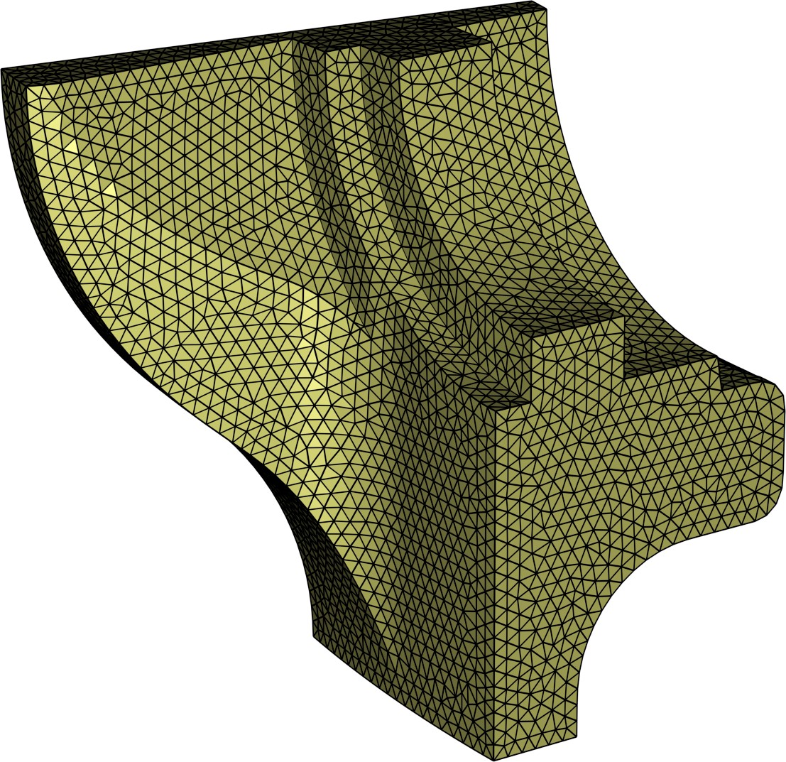
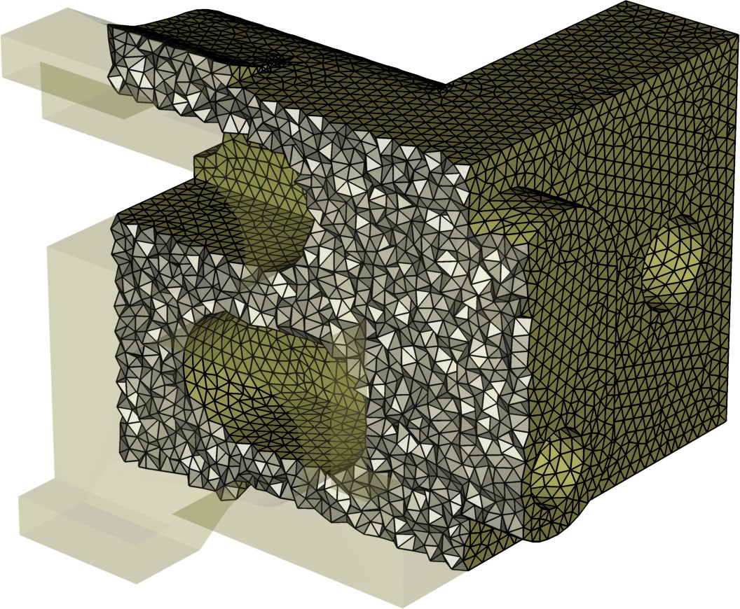
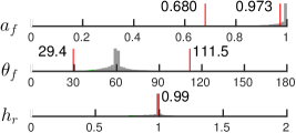
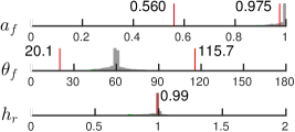
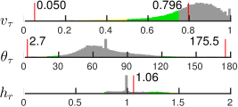
(CGAL-DR): $\,|\operatorname{Del}|_{\Sigma}\mathopen{}\mathclose{{}\left(X}\right)|=7,208,\,t=0.52\,\mathrm{sec}$	(CGAL-DR): $\,|\operatorname{Del}|_{\Sigma}\mathopen{}\mathclose{{}\left(X}\right)|=9,100,\,t=1.45\,\mathrm{sec}$	(CGAL-DR): $|\operatorname{Del}|_{\Omega}\mathopen{}\mathclose{{}\left(X}\right)|=137,899,\,t=2.97\,\mathrm{sec}$

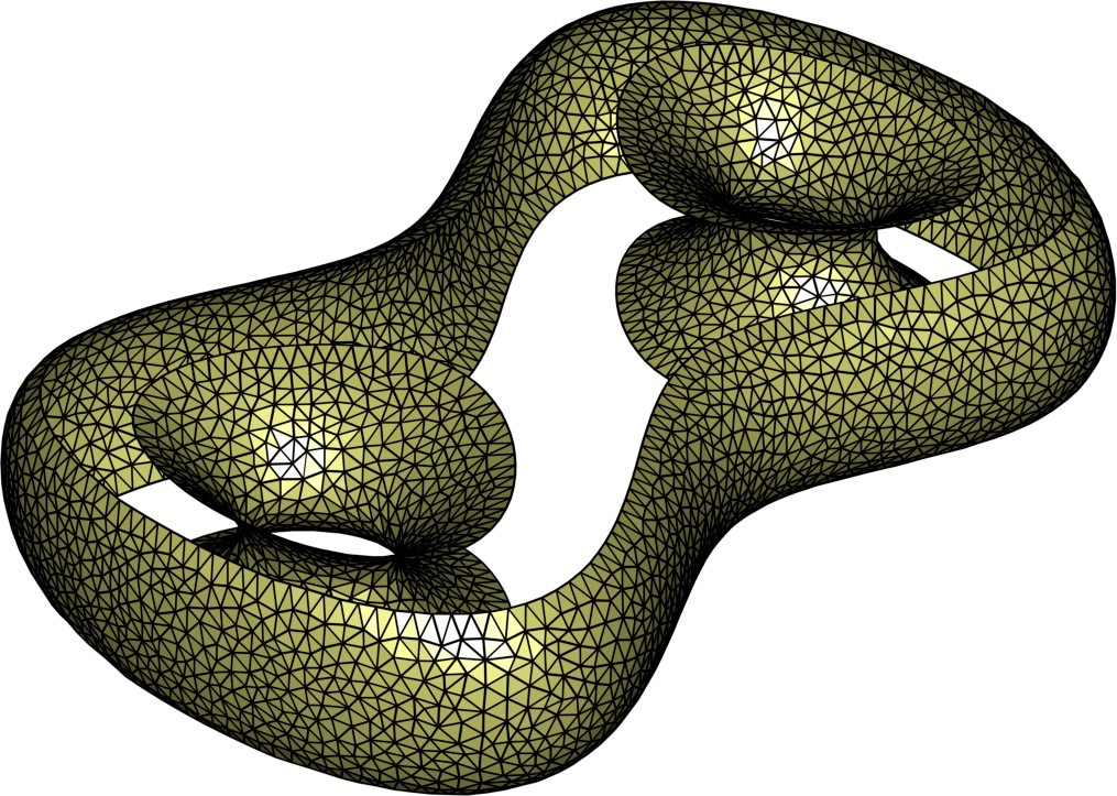
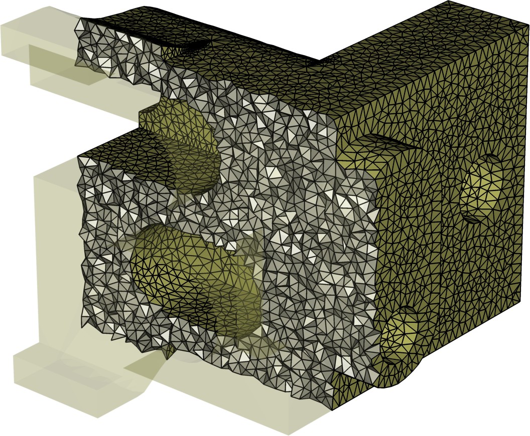
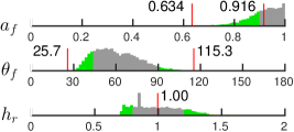
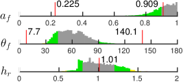
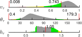
Figure 3: Meshes for the ISO, FANDISK and BRACKET test-cases, showing output for the JGSW-FD and CGAL-DR algorithms. Detailed mesh statistics are shown including normalised histograms of element area-length and volume-length ratios, dihedral-angles and relative edge-lengths. Element counts and total refinement times are also shown.

7.1 Preliminaries

The JGSW-FD and CGAL-DR algorithms were used to mesh a set of surface- and volume-based benchmark problems (Figure 3), comprising the ISO, FANDISK and BRACKET test-cases. The ISO test-case is an iso-surface problem, consisting of a multiply-connected collection of smooth surface patches with 1-dimensional constraints at the open boundary contours. The FANDISK object is a piecewise smooth surface model of a turbine component, incorporating a network of curve constraints inscribed at connections between adjacent surface patches. The FANDISK problem also includes sharply acute angle constraints, with a minimum angle of $20.1^{\circ}$ subtended by segments in the input geometry. The BRACKET object is a discrete CAD representation of a mechanical component, incorporating curve constraints at connections between adjacent surface patches, as per the FANDISK example. The BRACKET problem also incorporates acute angle constraints, with curve segments in the input geometry subtending angles as small as $6.5^{\circ}$.

In all test cases, constant radius-edge ratio thresholds were specified for both surface and volume elements, such that $\bar{\rho}_{f}=1.25$ and $\bar{\rho}_{\tau}=2$, corresponding to $\theta_{\text{min}}\geq 23.5^{\circ}$ for surface facets. Additionally, uniform mesh-size and surface discretisation constraints were enforced, setting $\bar{h}(\mathbf{x})=\alpha$ and $\bar{\epsilon}(\mathbf{x})=\beta\bar{h}\mathopen{}\mathclose{{}\left(\mathbf{x}}\right)$, with $\beta=\nicefrac{{1}}{{4}}$ and $\alpha$ a scalar length equivalent to approximately 3% of the mean bounding-box dimension associated with each input geometry. The JGSW-FD and CGAL-DR algorithms impose mesh-size constraints in a slightly different manner, with JGSW-FD treating $\bar{h}(\mathbf{x})$ as a constraint on edge-length, and CGAL-DR treating $\bar{h}(\mathbf{x})$ as a constraint on the radii of the circumscribing balls associated with each edge, triangle or tetrahedron. To compensate for this difference, the mesh-size targets associated with triangles and tetrahedrons in CGAL-DR were reduced by a factor of $\nicefrac{{4}}{{3}}$. Note that such scaling ensures that JGSW-FD and CGAL-DR produce output with equivalent mean edge length metrics.

For all test problems, detailed statistics on element quality are presented, including histograms of element volume-length and area-length ratios $v(\tau)$ and $a(f)$, element-angles $\theta(\tau)$ and $\theta(f)$, and relative-edge-length $\bar{h}_{r}$. The element volume-length and area-length ratios are robust measures of element quality, where high-quality elements attain scores that approach unity. The relative edge-length is defined to be the ratio of the measured edge-length $\|\mathbf{e}\|$ to the target value $\bar{h}(\mathbf{x}_{e})$, where $\mathbf{x}_{e}$ is the edge midpoint. Relative edge-lengths close to unity indicate conformance to the mesh-size function. High-quality surface triangles and interior tetrahedrons contain angles of $60.0^{\circ}$ and $70.5^{\circ}$ respectively.

7.2 A Comparison of JGSW-FD and CGAL-DR

The results in Figure 3 show that, overall, the new JGSW-FD algorithm typically outperforms the CGAL-DR implementation – generating slightly smaller meshes with improved element quality characteristics and mesh-size conformance. Overall computational expense for both algorithms was observed to be similar. In terms of element counts, the new method leads to a reduction of approximately 6%. Focusing on the distributions of element shape-quality, it can be seen that the JGSW-FD algorithm achieves significant improvements in mean area-length and plane-angle distributions in the case of the ISO and FANDISK problems, with smaller improvements in the volume-length and dihedral-angle metrics realised in the BRACKET test-case. In all cases, it can be seen that tight, high-quality distributions ($a_{f}\simeq 1$, $v_{\tau}\simeq 1$ and $\theta_{f}\simeq 60^{\circ}$, $\theta_{\tau}\simeq 70^{\circ}$) are generated by the Frontal-Delaunay algorithm (JGSW-FD), while the standard Delaunay-refinement approach (CGAL-DR) leads to broad, lower-quality distributions about similar means. Comparisons of distributions of element relative-length reveal the largest relative differences between algorithms, with the JGSW-FD implementation showing significantly improved conformance to the imposed mesh-size function, seen as a tight clustering of $h_{r}\simeq 1$ in all test-cases. This result is not unexpected – confirming that the new size-optimal off-centre point-placement scheme leads to high-quality vertex distributions that follow the imposed sizing function. These results are consistent with those previously obtained by the author for smooth manifold geometries [1, 2] using a simplified version of the three-dimensional Frontal-Delaunay-refinement algorithm presented here. These results demonstrate that the restricted Frontal-Delaunay paradigm can be extended to support piecewise smooth geometric inputs, including collections of curves, surfaces and enclosed volumes.

Differences were also observed in the manner in which the JGSW-FD and CGAL-DR algorithms protect sharp 1-dimensional features. Specifically, in the case of the FANDISK and BRACKET test problems, it was seen that the static protecting-balls strategy utilised in the CGAL-DR algorithm led to significant local over-refinement, even creating elements with smaller angles than those imposed by the geometry itself. In contrast, the protecting-collar approach developed in the current work, and deployed in the JGSW-FD, algorithm was observed to introduce a single isosceles element at the apex of any sharp 1-dimensional features, consistent with the methodology outlined in Section 5. In JGSW-FD, an associated local refinement of elements adjacent to these constraints is employed only to ensure that restricted edges are locally 1-manifold, typically leading to coarser local meshes. Overall, it is argued that the protecting-collar techniques developed in the current work offer a sparser and higher-quality solution to the problem of embedding arbitrary 1-dimensional constraints in restricted Delaunay meshes. Additional work focused on the development of high-quality protecting-collars for problems involving sharp surface features is currently in progress.

Acknowledgements. This work was conducted at the Massachusetts Institute of Technology and the University of Sydney with the support of a NASA–MIT cooperative agreement and an Australian Postgraduate Award. The author wishes to thank the anonymous reviewers for their helpful comments and feedback.

References

-
[1]
D. Engwirda, D. Ivers,
Off-centre
Steiner points for Delaunay-refinement on curved surfaces,
Computer-Aided Design 72 (2016) 157 – 171, 23rd International Meshing
Roundtable Special Issue: Advances in Mesh Generation.
doi:http://dx.doi.org/10.1016/j.cad.2015.10.007.
URL http://www.sciencedirect.com/science/article/pii/S0010448515001608 -
[2]
D. Engwirda,
Voronoi-based
Point-placement for Three-dimensional Delaunay-refinement, Procedia
Engineering 124 (2015) 330 – 342, 24th International Meshing Roundtable.
doi:http://dx.doi.org/10.1016/j.proeng.2015.10.143.
URL http://www.sciencedirect.com/science/article/pii/S1877705815032440 - [3] D. Engwirda, Locally optimal Delaunay-refinement and optimisation-based mesh generation, Ph.D. thesis, Department of Mathematics and Statistics, Sydney, Australia (2014).
- [4] S. W. Cheng, T. K. Dey, J. R. Shewchuk, Delauay Mesh Generation, Taylor & Francis, New York, 2013.
- [5] L. P. Chew, Guaranteed-quality Triangular Meshes, Tech. rep., Cornell University, Department of Computer Science, Ithaca, New York (1989).
- [6] J. Ruppert, A New and Simple Algorithm for Quality 2-dimensional Mesh Generation, in: Proceedings of the fourth annual ACM-SIAM Symposium on Discrete algorithms, SODA ’93, Society for Industrial and Applied Mathematics, Philadelphia, PA, USA, 1993, pp. 83–92.
- [7] J. Ruppert, A Delaunay Refinement Algorithm for Quality 2-Dimensional Mesh Generation, Journal of Algorithms 18 (3) (1995) 548 – 585. doi:http://dx.doi.org/10.1006/jagm.1995.1021.
- [8] J. R. Shewchuk, Delaunay Refinement Mesh Generation, Ph.D. thesis, School of Computer Science, Pittsburg, Pennsylvania (1997).
- [9] J. R. Shewchuk, Tetrahedral Mesh Generation by Delaunay Refinement, in: Proceedings of the fourteenth annual symposium on Computational geometry, SCG ’98, ACM, New York, NY, USA, 1998, pp. 86–95.
- [10] S. Cheng, T. Dey, Quality Meshing with Weighted Delaunay Refinement, SIAM Journal on Computing 33 (1) (2003) 69–93.
- [11] S. W. Cheng, T. K. Dey, E. A. Ramos, Delaunay Refinement for Piecewise Smooth Complexes, Discrete & Computational Geometry 43 (1) (2010) 121–166.
- [12] J. D. Boissonnat, S. Oudot, Provably Good Surface Sampling and Approximation, in: ACM International Conference Proceeding Series, Vol. 43, 2003, pp. 9–18.
- [13] J. D. Boissonnat, S. Oudot, Provably Good Sampling and Meshing of Surfaces, Graphical Models 67 (5) (2005) 405–451.
- [14] C. Jamin, P. Alliez, M. Yvinec, J.-D. Boissonnat, CGALmesh: a generic framework for delaunay mesh generation, ACM Transactions on Mathematical Software (TOMS) 41 (4) (2015) 23.
- [15] H. Si, Constrained Delaunay Tetrahedral Mesh Generation and Refinement, Finite Elements in Analysis and Design 46 (1–2) (2010) 33 – 46, mesh Generation - Applications and Adaptation.
- [16] H. Si, TetGen, a Delaunay-Based Quality Tetrahedral Mesh Generator, ACM Trans. Math. Softw. 41 (2) (2015) 11:1–11:36.
- [17] H. Edelsbrunner, N. R. Shah, Triangulating Topological Spaces, International Journal of Computational Geometry & Applications 7 (04) (1997) 365–378.
- [18] J. R. Shewchuk, General-dimensional Constrained Delaunay and Constrained Regular Triangulations, I: Combinatorial Properties, Discrete & Computational Geometry 39 (1-3) (2008) 580–637.
- [19] H. Si, Adaptive Tetrahedral Mesh Generation by Constrained Delaunay Refinement, International Journal for Numerical Methods in Engineering 75 (7) (2008) 856–880.
- [20] L. Rineau, M. Yvinec, Meshing 3D Domains Bounded by Piecewise Smooth Surfaces, in: M. L. Brewer, D. Marcum (Eds.), Proceedings of the 16th International Meshing Roundtable, Springer Berlin Heidelberg, Berlin, Heidelberg, 2008, pp. 443–460.
- [21] S. W. Cheng, T. K. Dey, J. A. Levine, A Practical Delaunay Meshing Algorithm for a Large Class of Domains, in: Proceedings of the 16th international meshing roundtable, Springer, 2008, pp. 477–494.
- [22] S. Oudot, L. Rineau, M. Yvinec, Meshing Volumes Bounded by Smooth Surfaces, in: Proceedings of the 14th International Meshing Roundtable, Springer, 2005, pp. 203–219.
- [23] C. Jamin, S. Pion, M. Teillaud, 3D Triangulations, in: CGAL User and Reference Manual, 4.6.1 Edition, CGAL Editorial Board, 2015.
- [24] A. Bowyer, Computing Dirichlet Tessellations, The Computer Journal 24 (2) (1981) 162–166.
- [25] P. Alliez, S. Tayeb, C. Wormser, AABB Tree, Tech. rep. (2009).
- [26] H. Erten, A. Üngör, Quality Triangulations with Locally Optimal Steiner Points, SIAM J. Sci. Comp. 31 (3) (2009) 2103–2130.
- [27] S. Rebay, Efficient Unstructured Mesh Generation by Means of Delaunay Triangulation and Bowyer-Watson Algorithm, Journal of Computational Physics 106 (1) (1993) 125 – 138.
- [28] D. J. Mavriplis, An Advancing Front Delaunay Triangulation Algorithm Designed for Robustness, Journal of Computational Physics 117 (1) (1995) 90 – 101.
- [29] P. J. Frey, H. Borouchaki, P. L. George, 3D Delaunay Mesh Generation Coupled with an Advancing-Front Approach, Computer Methods in Applied Mechanics and Engineering 157 (1–2) (1998) 115 – 131.
- [30] J. F. Remacle, F. Henrotte, T. Carrier-Baudouin, E. Béchet, E. Marchandise, C. Geuzaine, T. Mouton, A Frontal-Delaunay Quad-Mesh Generator using the -norm, International Journal for Numerical Methods in Engineering 94 (5) (2013) 494–512.
- [31] P. A. Foteinos, A. N. Chernikov, N. P. Chrisochoides, Fully generalized two-dimensional constrained delaunay mesh refinement, SIAM Journal on Scientific Computing 32 (5) (2010) 2659–2686.
- [32] A. N. Chernikov, N. P. Chrisochoides, Generalized insertion region guides for delaunay mesh refinement, SIAM Journal on Scientific Computing 34 (3) (2012) A1333–A1350.
- [33] S. E. Pav, N. J. Walkington, Delaunay refinement by corner lopping, in: Proceedings of the 14th International Meshing Roundtable, Springer, 2005, pp. 165–181.
- [34] A. Rand, N. Walkington, 3d Delaunay refinement of sharp domains without a local feature size oracle, in: Proceedings of the 17th International Meshing Roundtable, Springer, 2008, pp. 37–54.
- [35] A. Rand, N. Walkington, Collars and intestines: Practical conforming Delaunay refinement, in: Proceedings of the 18th International Meshing Roundtable, Springer, 2009, pp. 481–497.
- [36] S. W. Cheng, T. K. Dey, H. Edelsbrunner, M. A. Facello, S. H. Teng, Silver Exudation, J. ACM 47 (5) (2000) 883–904.
- [37] B. M. Klingner, J. R. Shewchuk, Aggressive Tetrahedral Mesh Improvement, in: M. L. Brewer, D. Marcum (Eds.), Proceedings of the 16th International Meshing Roundtable, Springer Berlin Heidelberg, 2008, pp. 3–23.
- [38] S. Gosselin, C. Ollivier-Gooch, Tetrahedral Mesh Generation using Delaunay Refinement with Non-standard Quality Measures, International Journal for Numerical Methods in Engineering 87 (8) (2011) 795–820.
- [39] D. Engwirda, JIGSAW: An unstructured mesh generation package, http://www.github.com/dengwirda/jigsaw-matlab (2016).
- [40] C. Jamin, S. Pion, M. Teillaud, 3D Triangulation Data Structure, in: CGAL User and Reference Manual, 4.6.1 Edition, CGAL Editorial Board, 2015.