T1600189

Analytical calculation of Hermite-Gauss and Laguerre-Gauss modes on a bullseye photodiode

 

1 Introduction

Some readers may be familiar with the use of a transversally split photodiode to measure the misalignment of a beam, effectively detecting the order 1 spatial modes incident on the photodiode. Using a similar method a radially split photodiode can be used to measure the mode mismatch of a beam, by detecting the order 2 spatial modes.

The idea of using a radially split, or ‘bullseye’ photodiode is not a new one; in fact it may be traced back at least to the original ‘wavefront sensing’ paper by Morrison et al. [1]. However, it was not until 2000 that Mueller et al. experimentally demonstrated the use of bullseye photodetectors in a closed loop for optimizing the mode-matching into a Fabry-Perot cavity [2].

Recently the issue of mode-mismatch sensing in Advanced LIGO has come to the fore [3]. Sensing mismatches with bullseye detectors in Advanced LIGO is a significantly more complex challenge than in a simple Fabry-Perot cavity, and so accurate simulation of the signals achieved is necessary. For this reason it has been necessary to derive the response of such detectors to optical beats between higher-order spatial modes.

This note describes the analytical derivation of the response of bullseye detectors to optical beats between higher-order spatial modes of the Laguerre-Gauss form, and subsequently the Hermite-Gauss form. Also included is a comparison with numerically calculated beat coefficients, and a simple example of the use of the resulting beat coefficients in simulating a mode mismatch sensor for a Fabry-Perot cavity.

2 Analytical derivation

2.1 The problem

To correctly calibrate the response of a bullseye photodiode we require the coefficients for beats between different higher order modes. We have two fields, the carrier and sidebands, each potentially made up of a combination of higher order modes. For the beat between two higher order modes, $u_{n,m}$ and $u_{n^{\prime},m^{\prime}}$, we consider a carrier field:

$$E_{\mathrm{c}}(r,\phi)=a_{n,m}u_{n,m}(r,\phi)$$ (1)

and a sideband field:

$$E_{\mathrm{sb}}(r,\phi)=a_{n^{\prime},m^{\prime}}u_{n^{\prime},m^{\prime}}(r,\phi)$$ (2)

The intensity of a combination of these fields becomes:

$$I(r,\phi)=|E_{\mathrm{c}}+E_{\mathrm{sb}}|^{2}=a_{n,m}u_{n,m}a_{n^{\prime},m^{\prime}}^{*}u_{n^{\prime},m^{\prime}}^{*}+a_{n,m}^{*}u_{n,m}^{*}a_{n^{\prime},m^{\prime}}u_{n^{\prime},m^{\prime}}+|a_{n,m}u_{n,m}|^{2}+|a_{n^{\prime},m^{\prime}}u_{n^{\prime},m^{\prime}}|^{2}$$ (3)

We are concerned with the components oscillating at the beat frequency between the carrier and sidebands. These are the components which include the cross terms, not the third and fourth terms which are simply DC components. Thus we can ignore them in our analysis for a demodulated signal. The signal generated by a bullseye photodiode is the difference between the signal generated in the outer and inner areas. For the terms at the beat frequency this is:

$$\begin{split}S{}&=a_{n,m}a_{n^{\prime},m^{\prime}}^{*}\int_{R}^{\infty}\int_{0}^{2\pi}u_{n,m}u^{*}_{n^{\prime},m^{\prime}}\ r\ \mbox{d}\phi\ \mbox{d}r\ +\ a_{n,m}^{*}a_{n^{\prime},m^{\prime}}\int_{R}^{\infty}\int_{0}^{2\pi}u^{*}_{n,m}u_{n^{\prime},m^{\prime}}\ r\ \mbox{d}\phi\ \mbox{d}r\\ {}&-\ a_{n,m}a_{n^{\prime},m^{\prime}}^{*}\int_{0}^{R}\int_{0}^{2\pi}u_{n,m}u^{*}_{n^{\prime},m^{\prime}}\ r\ \mbox{d}\phi\ \mbox{d}r\ -\ a_{n,m}^{*}a_{n^{\prime},m^{\prime}}\int_{0}^{R}\int_{0}^{2\pi}u^{*}_{n,m}u_{n^{\prime},m^{\prime}}\ r\ \mbox{d}\phi\ \mbox{d}r\\ {}&=c_{n,m,n^{\prime},m^{\prime}}\ a_{n,m}a_{n^{\prime},m^{\prime}}^{*}+c_{n^{\prime},m^{\prime},n,m}a_{n^{\prime},m^{\prime}}^{*}a_{n,m}\end{split}$$ (4)

where $c_{n,m,n^{\prime},m^{\prime}}$ is the beat coefficient between modes $n,m$ and $n^{\prime},m^{\prime}$.

2.2 Approach

As the active area of a bullseye photodiode is cylindrically symmetric it is sensible to approach this analysis using the cylindrically symmetric Laguerre-Gauss modes. There exists a conversion between the Laguerre and Hermite-Gauss basis, from which we can convert the analytical result for LG modes to that for the HG modes.

2.3 Calculating LG beat coefficients

In terms of LG modes we have the inner integral:

$$k_{p,l,p^{\prime},l^{\prime}}^{\mathrm{inner}}=\int_{0}^{R}\int_{0}^{2\pi}u_{p,l}u^{*}_{p^{\prime},l^{\prime}}\ r\mbox{d}\phi\ \mbox{d}r$$ (5)

and the outer integral:

$$k_{p,l,p^{\prime},l^{\prime}}^{\mathrm{outer}}=\int_{R}^{\infty}\int_{0}^{2\pi}u_{p,l}u^{*}_{p^{\prime},l^{\prime}}\ r\mbox{d}\phi\ \mbox{d}r$$ (6)

where $R$ is the radius of the inner circle of the bullseye photodiode. The Laguerre-Gauss mdoes are given by:

$$\begin{split}u_{p,l}(r,\phi,z){}&=\frac{1}{w(z)}\sqrt{\frac{2p!}{\pi(|l|+p)!}}\exp{({\rm i}\,(2p+|l|+1)\Psi(z))}\\ {}&\left(\frac{\sqrt{2}r}{w(z)}\right)^{|l|}L_{p}^{|l|}\left(\frac{2r^{2}}{w^{2}}\right)\exp{\left(-\frac{{\rm i}\,kr^{2}}{2R_{C}(z)}-\frac{r^{2}}{w^{2}(z)}+{\rm i}\,l\phi\right)}\end{split}$$ (7)

where $w$ is the beam spot size, $p$ and $l$ are the radial and azimuthal indices, $\Psi$ is the Gouy phase, $k$ is the wavenumber and $R_{C}$ is the radius of curvature of the wavefront. $L_{p}^{|l|}$ refer to the associated Laguerre polynomials.

We have:

$$u_{p,l}u^{*}_{p^{\prime},l^{\prime}}=\alpha\left(\frac{\sqrt{2}r}{w}\right)^{|l|+|l^{\prime}|}L_{p}^{|l|}\left(\frac{2r^{2}}{w^{2}}\right)L_{p^{\prime}}^{|l^{\prime}|}\left(\frac{2r^{2}}{w^{2}}\right)\exp{\left(-\frac{2r^{2}}{w^{2}}+{\rm i}\,(l-l^{\prime})\phi\right)}$$ (8)

where the complex constant $\alpha$ is given by:

$$\alpha=\frac{2}{w^{2}\pi}\sqrt{\frac{p!p^{\prime}!}{(|l|+p)!(|l^{\prime}|+p^{\prime})!}}\exp{({\rm i}\,(2p+|l|-2p^{\prime}-|l^{\prime}|)\Psi)}$$ (9)

It is convenient to include the Gouy phase explicitly in this form, because in Finesse simultion the Gouy phase is stored in the amplitude coefficients for the modes and we need to remove it from the beat coefficients computation.

The integral can be easily separated into the two variables $r$ and $\phi$. For the angular integration we simply have:

$$I_{\phi}=\int_{0}^{2\pi}\exp{({\rm i}\,(l-l^{\prime})\phi)}\mathrm{d}\phi=\left[\frac{e^{{\rm i}\,(l-l^{\prime})\phi}}{{\rm i}\,(l-l^{\prime})}\right]_{0}^{2\pi}=0$$ (10)

The only non-zero result is achieved when $l=l^{\prime}$, i.e. when the exponential drops out before the integration. In this case:

$$I_{\phi}(l=l^{\prime})=2\pi$$ (11)

This is a useful result as it shows that the beats between any two modes with $l\neq l^{\prime}$ do not contribute for the case of a bullseye photodiode. This makes sense as the active area of the photodiode has no angular dependence.

We now consider the radial integration:

$$I_{r}=\int_{a}^{b}\left(\frac{\sqrt{2}r}{w}\right)^{2|l|}L_{p}^{|l|}\left(\frac{2r^{2}}{w^{2}}\right)L_{p^{\prime}}^{|l|}\left(\frac{2r^{2}}{w^{2}}\right)\exp{\left(-\frac{2r^{2}}{w^{2}}\right)}\ r\ \mbox{d}r$$ (12)

where $a$ and $b$ represent the limits for the integration for either the inner ($a=0$, $b=R$) or outer ($a=R$, $b=\infty$) ring and we use $l=l^{\prime}$ as the only non-zero contribution. We now make a variable substitution:

$$\begin{matrix}x=\frac{2r^{2}}{w^{2}}&\ \ \ \ \ &\mbox{d}r=\frac{w^{2}}{4r}\ \mbox{d}x\\ \end{matrix}$$ (13)

We now have:

$$I_{r}=\int_{A}^{B}x^{|l|}L_{p}^{|l|}(x)L_{p^{\prime}}^{|l|}(x)\exp(-x)\ \mbox{d}x$$ (14)

where $A$ and $B$ are the new limits of the integral, $A=0$, $B=\frac{2R^{2}}{w^{2}}$ for the inner integral and $A=\frac{2R^{2}}{w^{2}}$, $B=\infty$ for the outer integral. The associated Laguerre polynomials are of the form:

$$L_{p}^{|l|}(x)=\sum_{i=0}^{p}(-1)^{i}\frac{(p+|l|)!}{(p-i)!(|l|+i)!i!}x^{i}$$ (15)

We end up trying to integrate a function of the form $x^{n}e^{-x}$ for each term in the two Laguerre sums:

$$I_{r}=\frac{w^{2}}{4}(p+|l|)!(p^{\prime}+|l|)!\sum_{i=0}^{p}\sum_{j=0}^{p^{\prime}}(-1)^{i+j}\int_{A}^{B}\frac{x^{|l|+i+j}e^{-x}}{(p-i)!(p^{\prime}-j)!(|l|+i)!(|l|+j)!i!j!}\mbox{d}x$$ (16)

In the case of the limits on the integration for the inner and outer integration, this integral can be solved using the lower (inner) and upper (outer) incomplete gamma functions. The lower incomplete gamma function has the form:

$$\gamma(n,x)=\int_{0}^{x}t^{n-1}e^{-t}\ \mbox{d}t=(n-1)!\left(1-e^{-x}\sum_{k=0}^{n-1}\frac{x^{k}}{k!}\right)$$ (17)

for integer $n$. The upper incomplete gamma function is given by:

$$\Gamma(n,x)=\int_{x}^{\infty}t^{n-1}e^{-t}\ \mbox{d}t=(n-1)!\ e^{-x}\sum_{k=0}^{n-1}\frac{x^{k}}{k!}$$ (18)

So the beat coefficients in terms of Laguerre-Gauss modes can be written as:

$$\begin{split}c_{p,l,p^{\prime},l^{\prime}}{}&=k^{\mathrm{outer}}_{p,l,p^{\prime},l^{\prime}}-k^{\mathrm{inner}}_{p,l,p^{\prime},l^{\prime}}\\ {}&=\delta_{l,l^{\prime}}\sqrt{p!p^{\prime}!(|l|+p)!(|l|+p^{\prime})!}\exp{({\rm i}\,(2p-2p^{\prime})\Psi)}\left[\sum_{i=0}^{p}\sum_{j=0}^{p^{\prime}}\frac{(-1)^{i+j}\Gamma\left(|l|+i+j+1,\frac{2R^{2}}{w^{2}}\right)}{(p-i)!(p^{\prime}-j)!(|l|+i)!(|l|+j)!i!j!}\right.\\ {}&-\left.\sum_{i=0}^{p}\sum_{j=0}^{p^{\prime}}\frac{(-1)^{i+j}\gamma\left(|l|+i+j+1,\frac{2R^{2}}{w^{2}}\right)}{(p-i)!(p^{\prime}-j)!(|l|+i)!(|l|+j)!i!j!}\right]\end{split}$$ (19)

where $d_{l,l^{\prime}}$ is the Kronecker delta, fulfilling the condition of non zero results only when $l=l^{\prime}$.

2.4 Converting to HG beat coefficients

Any HG mode can be expressed as a sum of LG modes:

$$u_{n,m}=\sum_{p,l}a_{p,l}u_{p,l}$$ (20)

where the sum over $p$ and $l$ refers to a sum over all the LG modes with the same order as the desired HG mode, i.e. $n+m=2p+|l|$. See [4] for a detailed description of this conversion.

Thus we can write the overlap of two HG modes on a bullseye photodiode in terms of LG modes. For example, the inner overlap is given as:

$$k^{\mathrm{inner}}_{n,m,n^{\prime},m^{\prime}}=\int_{0}^{R}\int_{0}^{2\pi}u_{n,m}u^{*}_{n^{\prime},m^{\prime}}\ r\ \mbox{d}\phi\ \mbox{d}r=\int_{0}^{R}\int_{0}^{2\pi}\sum_{p,l}a_{p,l}u_{p,l}\sum_{p^{\prime},l^{\prime}}a^{*}_{p^{\prime},l^{\prime}}u_{p^{\prime},l^{\prime}}^{*}r\ \mbox{d}\phi\ \mbox{d}r$$ (21)

We can now use the solutions of the integrals derived in the previous section. The equation is simplified as the only non-zero contributions come from the terms in the sum with $l=l^{\prime}$, as shown in the previous section. This removes a lot of terms in the integral and we finally have:

$$k^{\mathrm{inner}}_{n,m,n^{\prime},m^{\prime}}=\sum_{l}a_{p,l}a^{*}_{p^{\prime},l}k^{\mathrm{inner}}_{p,l,p^{\prime},l}$$ (22)

where we sum over only the $l$ values which appear in the expansions of both Hermite-Gauss modes ($l=l^{\prime}$). To determine the range of $l$ we consider an example beat between two modes of different orders, the HG₀₂ mode and HG₂₂ mode. These modes can be expressed in terms of LG modes or order 2 for HG₀₂:

$$\mbox{HG}_{02}=-0.5\times\mbox{LG}_{0-2}-0.7071\times\mbox{LG}_{10}-0.5\times\mbox{LG}_{02}$$ (23)

and order 4 for HG₂₂:

$$\mbox{HG}_{22}=0.25\times\mbox{LG}_{0-4}+0.5\times\mbox{LG}_{1-2}+0.6124\times\mbox{LG}_{20}+0.5\times\mbox{LG}_{12}+0.25\times\mbox{LG}_{04}$$ (24)

To calculate the beat between these two modes we need only consider the LG modes with $l=l^{\prime}$. In this example the azimuthal indices common to both expansions are $l=-2$, $l=0$ and $l=2$. So we only need these 3 terms in our calculation of the beat coefficient. Consider instead the beat between HG₀₂ and the order 3 mode, HG₂₁, which can be expressed as:

$$\mbox{HG}_{21}=0.6124{\rm i}\,\times\mbox{LG}_{0-3}-0.3536{\rm i}\,\times\mbox{LG}_{1-1}+0.3536{\rm i}\,\times\mbox{LG}_{11}-0.6124{\rm i}\,\times\mbox{LG}_{03}$$ (25)

In this case there are no common $l$ modes between the two modes and the beat is zero. This is the case for all modes when the difference between the orders is odd. In the case where the difference between the mode orders is even we have $l=l^{\prime}=-O_{\mathrm{min}},-O_{\mathrm{min}}+2,-O_{\mathrm{min}}+4,\dots O_{\mathrm{min}}$, where $O_{\mathrm{min}}$ is the smaller of the two orders.

3 Example Coefficients

3.1 Derived beat coefficients for an optimally sized beam

The formula given in eqn. 22 can be used to calculate the beat coefficients as measured by a bullseye photodetector between all HG modes up to a specified order. The beat coefficients calculated in this way are printed up to mode order 3 in table 1, for the specific case where the radius of the inner portion of the detector relative to the incident beam radius is chosen such that the HG₀₀ $\times$ HG₀₀ beat coefficient is negligibly small. In practise this should mean that the total power falling inside the inner portion of the detector is equal to the total power falling in the outer portion.

The detector inner portion radius relative to beam radius required to achieve this condition was found to be $0.5887050112577$.

n	m	n′	m′	coeff.
0	0	0	2	0.490129071734255
0	0	2	0	0.490129071734255
0	0	2	2	-0.226460336800429
0	1	0	1	0.693147180560006
0	1	0	3	0.294216182370426
0	1	2	1	0.169865792091509
0	1	2	3	-0.159974289570813
0	2	0	2	0.706913350718638
0	2	2	2	0.134069741206516
0	3	0	3	0.711794198742489
0	3	2	3	0.15405930406129
1	0	1	0	0.693147180560006
1	0	1	2	0.169865792091509
1	0	3	0	0.294216182370426
1	0	3	2	-0.159974289570813
1	1	1	1	0.933373687519067
1	1	1	3	0.0679783724283818
1	1	3	1	0.0679783724283818
1	1	3	3	-0.0688289693357714
1	2	1	2	0.896516597036745
1	2	3	2	0.0967993502022488
1	3	1	3	0.929666955955726
1	3	3	3	0.0707108474910448
2	0	2	0	0.706913350718638
2	0	2	2	0.134069741206516
2	1	2	1	0.896516597036745
2	1	2	3	0.0967993502022488
2	2	2	2	0.920269481591934
2	3	2	3	0.907333325165518
3	0	3	0	0.711794198742489
3	0	3	2	0.15405930406129
3	1	3	1	0.929666955955726
3	1	3	3	0.0707108474910448
3	2	3	2	0.907333325165518
3	3	3	3	0.927829909543617

Table 1: Analytically calculated bullseye detector HG beat coefficients up to order 3.

3.2 Comparison with numerically calculated beat coefficients

In order to test the validity of the analytical results, a numerical calculation of beat coefficients was also performed. In this calculation, the transversal amplitude functions of selected HG modes were generated to fill a 2D matrix. The coherent sum of two such amplitude functions was calculated and ‘dc terms’ were discarded, just as in the steps immediately following eqn. 3. Finally, the elements of the resulting matrix were summed for the outer and inner segments of the bullseye detector area and the difference between the total contributions in the inner and outer areas found.

This numerical beat coefficient calculation was performed for a few different combinations of HG modes, and for each combination for a range of different grid resolutions. The grid size relative to the beam radius was a constant at 10, and was always verified to be large enough such that greater than 99.9% of the power of both modes was within the grid area.

A comparison between the analytically derived results for a few different HG mode beat coefficients is shown in Fig. 1. As the grid resolution increases, the numerical results tend towards the analytical results for each of the 5 different HG mode combinations considered.

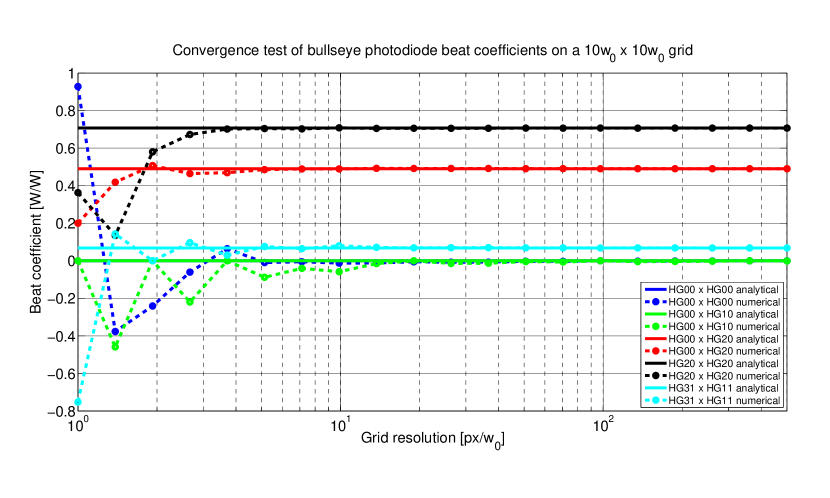
Figure 1: A comparison between beat coefficients obtained by the analytical result in eqn. 22, and those obtained by numerical integration. As the grid resolution used for the numerical integration is increased, the result tends to that provided by the analytical solution.

4 Demonstration of bullseye sensing in Finesse

In order to see how the derived bullseye detector beat coefficients can be used for the purposes of simulating a mode-mismatch sensing scheme, a simple example simulation was performed with the software Finesse [5]. Figure 2 shows the optical layout of the simulation.

A laser is phase modulated at 9 MHz to a modulation index of 0.1 by an EOM, before being made incident on a plane-concave Fabry-Perot cavity. The cavity length is 1 m and the concave end mirror has a radius of curvature of 2 m, giving a cavity eigenmode waist of 582 $\mu$m located at the flat input mirror. The cavity input mirror transmission is 1% and the end mirror transmission is 0.1%, putting the cavity in the overcoupled regime.

The light reflected from the cavity is picked off by a beam splitter, before being split again by a second beam splitter. The transmitted light from the second beam splitter is detected with a bullseye detector BPD1. The distance from the cavity input mirror to BPD1 is set to 0 m, so that BPD1 is effectively located at the cavity waist. The reflected light from the second beam splitter is sent to a second bullseye detector, BPD2, located at a distance 1 m from the cavity waist. Since the cavity eigenmode Rayleigh range is 1 m, this fixes the Gouy phase difference between the two bullseye detectors to be 45^∘.

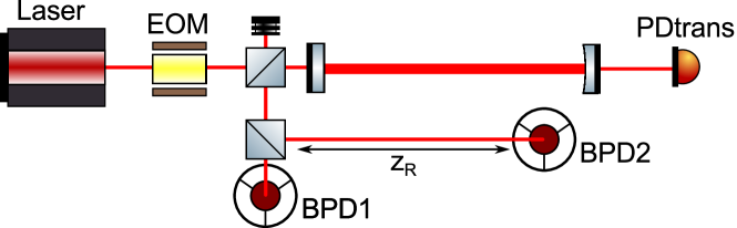
Figure 2: Optical layout of the bullseye photodetector simulation example. BPD1 is located at the nominal waist location of the cavity eigenmode, and BPD2 is one Rayleigh range away from the waist location. This gives a 45^∘ Gouy phase separation between BPD1 and BPD2.

The bullseye detectors are demodulated at the 9 MHz modulation frequency, with a demodulation phase that maximizes their sensitivity to any mismatch between the input beam mode and the cavity eigenmode. To test the response of the bullseye detectors to a mode mismatch between input beam and cavity mode, the beam parameters of the input beam are varied, using the gauss command in Finesse. The cavity beam parameters remain fixed throughout this variation of the input beam parameter, and thus the simulation represents a mode mismatch of the input beam into the cavity. The input beam waist location, and waist size (or equivalently Rayleigh range) are varied separately in order to observe the different response of BDP1 and BPD2 to these two types of mismatch. The maximum HG mode order considered in the simulation was 6.

The output signals from the two bullseye detectors are plotted in Fig. 3 as a function of the input beam waist location relative to the cavity waist (upper plot) and the input beam Rayleigh range (lower plot). The cavity transmitted light power is also shown in the plots. Here we see that BPD1 is primarily sensitive to the input beam waist location mismatch, whereas BPD2 is primarily sensitive to input beam waist size (or Rayleigh range) mismatch. We also see that both bullseye detector signals are linear in the region close to optimal mode matching, confirming that these would make appropriate error signals for use in a closed-loop feedback control system for mode matching the input beam to the cavity mode.

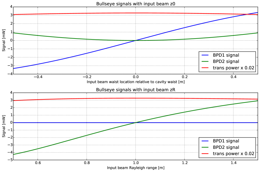
Figure 3: Simulated bullseye detector signals as a function of cavity input beam parameters, for a fixed cavity eigenmode. BPD1 is primarily sensitive to the input beam waist location mismatch, whereas BPD2 is primarily sensitive to input beam waist size (or Rayleigh range) mismatch.

5 Code to compute coefficients

The computation of beat coefficients for split and bullseye detectors has been added as a feature to our Python-based PyKat package [6]. To generate the default coefficients for Finesse to be stored in the kat.ini file, install Pykat and run:

import pykat.optics.pdtype as pdtype
pdtype.finesse_bullseye_photodiode(6)

References

- [1] E. Morrison, D. I. Robertson, H. Ward, and B. J. Meers. Automatic alignment of optical interferometers. Appl. Opt., 33:5041–5049, August 1994.
- [2] G. Mueller, Q.-Z. Shu, R. Adhikari, D. B. Tanner, D. Reitze, D. Sigg, N. Mavalvala, and J. Camp. Determination and optimization of mode matching into optical cavities by heterodyne detection. Optics Letters, 25:266–268, February 2000.
- [3] Aidan Brooks, Rana X. Adhikari, Stefan Ballmer, Lisa Barsotti, Paul Fulda, Antonio Perreca, and David Ottaway. Active wavefront control in and beyond advanced ligo. Technical report, LIGO, 2016. LIGO DCC number: LIGO-T1500188.
- [4] Charlotte Bond. How to stay in shape: Overcoming beam and mirror distortions in advanced gravitational wave interferometers. PhD thesis, University of Birmingham, June 2014.
- [5] A Freise, G Heinzel, H Lück, R Schilling, B Willke, and K Danzmann. Frequency-domain interferometer simulation with higher-order spatial modes. Classical and Quantum Gravity, 21(5):S1067–S1074, 2004. Finesse is available at http://www.gwoptics.org/finesse.
- [6] A. Freise D. Brown. Pykat, python interface and tools for Finesse. http://www.gwoptics.org/pykat/. Accessed: 2015-07-13.