Enhancing stability of correction procedure via reconstruction using summation-by-parts operators II: Modal filtering

Abstract

A recently introduced framework of semidiscretisations for hyperbolic conservation laws known as correction procedure via reconstruction (CPR, also known as flux reconstruction) is considered in the extended setting of summation-by-parts (SBP) operators using simultaneous approximation terms (SATs). This reformulation can yield stable semidiscretisations for linear advection and Burgers’ equation as model problems. In order to enhance these properties, modal filters are introduced to this framework. As a second part of a series, the results of Ranocha, Glaubitz, Öffner, and Sonar (Enhancing stability of correction procedure via reconstruction using summation-by-parts operators I: Artificial dissipation, 2016) concerning artificial dissipation / spectral viscosity are extended, yielding fully discrete stable schemes. Additionally, a new adaptive strategy to compute the filter strength is introduced and different possible applications of modal filters are compared both theoretically and numerically.

1 Introduction

Numerous phenomena in the field of engineering as well as natural sciences are modelled by partial differential equations (PDEs) and in particular by hyperbolic conservation laws. While being of vital significance, especially hyperbolic conservation laws are highly delicate from a mathematical point of view and often exact solutions are not known. Therefore, the study of numerical solutions is an important and interesting field of research.

In the last decades, great effort was made to develop special numerical schemes for these PDEs. Often the method of lines using a simple Runge-Kutta (RK) scheme in time is adapted [5, 7], where far most attention is given to suitable space discretisations. These can be obtained by well-known low order methods as well as high order ones, e.g. discontinuous Galerkin (DG), spectral difference (SD), recent flux reconstruction (FR) or correction procedure via reconstruction (CPR) methods. While the latter ones can provide highly desirable accuracy for smooth solutions, they are originally far less robust in the case of discontinuities than their low order counterparts. However, using summation-by-parts (SBP) operators along with simultaneous-approximation-terms (SATs) provably stable and conservative space discretesations in the FD framework were obtained. See for instance the review articles by [20, 16, 2]. In a similar manner their ideas have been extended to stable space discretisations for the CPR method by [19]. The FR method along with the CPR method as its generalisation provide a cell-wise spectral approach on a decomposition of the underlying domain, using correction terms at the cell boundaries quite similar to the SATs from the FD framework. Hence, by adapting analytical counterparts of the SBP operators using polynomial bases, also stable space discretisations for the FR and CPR method could be obtained.

Unfortunately, these stable space semidiscretisations alone cannot provide stable schemes in the fully discrete setting. Coming back to the decoupled time integration, already the explicit Euler method yealds an additional error after every time step.

This error might become most destructive when schemes using polynomial approximations like the CPR method are applied. Here, the Gibbs phenomenon will arise for solutions with jump discontinuities, and the method becomes unstable. There are several well-known solutions to enhance stability of a numerical scheme. In this work only the artificial dissipation or spectral viscosity method and modal filtering by certain exponential filters will be addressed. Artificial dissipation / spectral viscosity can be interpreted as discrete counterparts of the vanishing viscosity method. The latter one was originally used to prove the existence of entropy solutions by adding an iteratively decreasing viscosity term to the right hand side of the conservation law and constructing the $L_{1}$ limit of solutions to the resulting parabolic equation [8]. Since then, appropriate discretisations of such viscosity terms can be used to stabilise numerical schemes for hyperbolic conservation laws. If this discretisation is done in the FD framework, the corresponding method is often labelled artificial dissipation (AD) [12, 15] Using a method which approximates the solution polynomials however, the resulting method is then usually named spectral viscosity (SV) [9, 10, 11].

On the other hand, the idea of modal filtering exclusively adapts to such methods using series expansions [6]. This has already be done for DG methods by [13, 14] and for the SD method by [3]. At least for certain exponential filters, there is an equivalence to the spectral viscosity method, if a splitting in the time integration is used. In this work, both approaches are applied to the new CPR method using SBP operators. While this has already been done in various well-known schemes, this work is the first to do so in this particular recent one. Furthermore, the framework of SBP operators enables the study of different stabilisation approaches to the numerical solution and in particular to already mentioned errors from time integration schemes like the explicit Euler method. The authors make use of this by deriving completely new adaptive filtering techniques, which have not been published before to their best knowledge. While AV is addressed in the first part [17] of this series, this one focuses on modal filtering. Doing so, the rest is organised as follows:

In section 2 a brief introduction to the correction procedure via reconstruction using summation-by-parts operators is given. This recent method is proven to be conservative and stable for the problem of linear advection as well as for the non-linear Burgers’ equation using a skew-symmetric formulations for the discretisation. One should note however that the latter modal filtering approaches along with their analysis just require a stable space-discretisation using a polynomial approximation of the solution and thus are completely independent from this specific one.

This is stressed in the third section, when the idea of spectral viscosity and its connection to modal filtering is addressed. While part I of this work focused mainly on artificial dissipation, this part focuses on the idea of modal filtering and its strong relation by a certain operator splitting in time.

Naturally the question arises, when exactly modal filtering should be applied. Section 4 discusses the straight forward option of filtering in the sense of the above mentioned operator splitting, the fifth and sixth section address the potential of filtering the time derivative and filtering the solution.

The work is then completed by the authors’ conclusions and quite a few remarks about further research in the seventh section.

2 Correction procedure via reconstruction using summation-by-parts operators

In this section, a brief description of CPR methods using SBP operators will be given. Therefore, a one-dimensional scalar conservation law

$$\partial_{t}u+\partial_{x}f(u)=0,$$ (1)

equipped with an adequate initial condition will be used. For simplicity, periodic boundary conditions (or a compactly supported initial condition) will be assumed.

The domain is partitioned into subdomains, which are mapped diffeomorphically onto a reference element. Since only one spatial dimension is considered, these intervals can be mapped by an affine linear transformation. The following computations are done in this standard domain.

In the setting described by [18], the solution is represented as an element of a finite dimensional Hilbert space of functions on the volume. With respect to a chosen basis, the scalar product approximating the $L_{2}$ scalar product is represented by a matrix $\underline{\underline{M}}\,$ and the derivative (divergence) by $\underline{\underline{D}}\,$. Additionally, functions on the boundary (consisting of two points in this one dimensional case) are elements of another finite dimensional Hilbert space with appropriate basis. The restriction of functions on the volume to the boundary is represented by a (rectangular) matrix $\underline{\underline{R}}\,$ and integration with respect to the outer normal by $\underline{\underline{B}}\,$. Finally, the operators have to fulfil the SBP property

$$\underline{\underline{M}}\,\underline{\underline{D}}\,+\underline{\underline{D}}{{}^{T}}\underline{\underline{M}}\,=\underline{\underline{R}}{{}^{T}}\underline{\underline{B}}\,\underline{\underline{R}}\,$$ (2)

as compatibility condition in order to mimic integration by parts

$$\underline{u}^{T}\underline{\underline{M}}\,\underline{\underline{D}}\,\underline{v}+\underline{u}^{T}\underline{\underline{D}}{{}^{T}}\underline{\underline{M}}\,\underline{v}\approx\int_{\Omega}u\,\partial_{x}v+\int_{\Omega}\partial_{x}u\,v=u\,v\big{|}_{\partial\Omega}\approx\underline{u}^{T}\underline{\underline{R}}{{}^{T}}\underline{\underline{B}}\,\underline{\underline{R}}\,\underline{v}.$$ (3)

Additional ingredients of CPR methods are numerical fluxes (Riemann solvers) $f^{\mathrm{num}}$, computing a common flux on the boundary using values from both neighbouring elements, and a correction step, which [19] formulated as an SAT, similarly to the weak enforcement of boundary condition in finite difference SBP schemes.

In the following, polynomial bases will be used for functions on the volume, either nodal Gauß-Legendre / Lobatto-Legendre or modal Legendre bases. Multiplication of functions on the volume will be conducted pointwise for nodal bases or exactly, followed by an $L_{2}$ projection, for modal bases. The resulting multiplication operators are written with two underlines, e.g. $\underline{\underline{u}}\,$ represents multiplication with the polynomial given by $\underline{u}$.

2.1 Linear advection

A simple example for a scalar conservation law (1) is given by the linear advection equation with constant velocity

$$\partial_{t}u+\partial_{x}u=0.$$ (4)

The semidiscretisation using the canonical of the correction procedure can be written as

$$\partial_{t}\underline{u}=-\underline{\underline{D}}\,\underline{u}-\underline{\underline{M}}{{}^{-1}}\underline{\underline{R}}{{}^{T}}\underline{\underline{B}}\,\left(\underline{f}^{\mathrm{num}}-\underline{\underline{R}}\,\underline{u}\right)$$ (5)

in the reference domain. It is conservative across elements and stable if an appropriate numerical flux is applied, see inter alia Theorem 5 of [19].

2.2 Burgers’ equation

As a nonlinear model, Burgers’ equation

$$\partial_{t}u+\partial_{x}\frac{u^{2}}{2}=0$$ (6)

is more difficult to handle correctly, since discontinuities may develop in finite time. However, a conservative (across elements) and stable (with respect to the discrete norm induced by $\underline{\underline{M}}\,$) semidiscretisation can be obtained by the application of a skew-symmetric form

$$\partial_{t}\underline{u}=-\frac{1}{3}\underline{\underline{D}}\,\underline{\underline{u}}\,\underline{u}-\frac{1}{3}\underline{\underline{u}}\,{{}^{*}}\underline{\underline{D}}\,\underline{u}+\underline{\underline{M}}{{}^{-1}}\underline{\underline{R}}{{}^{T}}\underline{\underline{B}}\,\left(\underline{f}^{\mathrm{num}}-\frac{1}{3}\underline{\underline{R}}\,\underline{\underline{u}}\,\underline{u}-\frac{1}{6}\left(\underline{\underline{R}}\,\underline{u}\right)^{2}\right),$$ (7)

if the numerical flux is adequate, see inter alia Theorem 2 of [18].

3 Spectral viscosity and modal filtering

In this section, spectral viscosity will be briefly introduced as a means to improve stability properties not influencing conservation across elements. Using the Sturm-Liouville operator associated with Legendre polynomials for artificial dissipation, the continuous properties for polynomial bases are investigated in the discrete setting and modal filters are derived by a classical operator splitting approach.

3.1 Spectral viscosity in the continuous and semidiscrete setting

A spectral viscosity extension of a scalar conservation law (1) can be written as

$$\partial_{t}u(t,x)+\partial_{x}f(u(t,x))=(-1)^{s+1}\varepsilon\left(\partial_{x}a(x)\partial_{x}\right)^{s}u(t,x),$$ (8)

introducing the strength $\varepsilon\geq 0$, the order $s\in\mathbb{N}$, and a suitable polynomial $a\colon\mathbb{R}\to\mathbb{R}$, fulfilling $a\big{|}\Omega\geq 0$ and $a\big{|}_{\partial\Omega}=0$. Then, conservation across the element $\Omega$ is preserved and the artificial dissipation on the right hand side enforces an additional decay of the $L_{2}$ norm of the solution $u$, as described inter alia by [17] in section 3.1.

In order to enforce the same properties in the semidiscrete setting, the artificial dissipation should be discretised as

$$(-1)^{s+1}\varepsilon\left(-\underline{\underline{M}}{{}^{-1}}\underline{\underline{D}}{{}^{T}}\underline{\underline{M}}\,\underline{\underline{a}}\,\underline{\underline{D}}\,\right)^{s}\underline{u}=-\varepsilon\left(\underline{\underline{M}}{{}^{-1}}\underline{\underline{D}}{{}^{T}}\underline{\underline{M}}\,\underline{\underline{a}}\,\underline{\underline{D}}\,\right)^{s}\underline{u},$$ (9)

see inter alia section 3.2 of [17]. Additionally, they prove

Lemma 1 (Lemma 2 of [17]).

The discrete viscosity operator $-\underline{\underline{M}}{{}^{-1}}\underline{\underline{D}}{{}^{T}}\underline{\underline{M}}\,\underline{\underline{a}}\,\underline{\underline{D}}\,u$ of the right hand side (9)

• has the correct eigenvalues $-n(n+1)$ with eigenvectors given by the Legendre polynomials $\varphi_{n},n\in\mathinner{\left\{0,\dots,p\right\}}$ if a modal Legendre or a nodal Gauß-Legendre basis is used. These eigenvalues and eigenvectors are the same as the ones of the continuous operator $\partial_{x}(1-x^{2})\partial_{x}$.

• has the correct eigenvalues $-n(n+1)$ with eigenvectors given by the Legendre polynomials $\varphi_{n},n\in\mathinner{\left\{0,\dots,p-1\right\}}$, if a nodal Lobatto-Legendre basis is used. The eigenvalue for $\varphi_{p}$ is non-positive and bigger than $-p(p+1)$, i.e. the artificial viscosity operator yields less dissipation of the highest mode compared to the exact value, obtained by modal Legendre and nodal Gauß-Legendre bases.

3.2 Discrete setting

In order to discretise the augmented conservation law (8)

$$\partial_{t}u+\partial_{x}f(u)=\varepsilon\,\partial_{x}a(x)\partial_{x}u$$ (10)

with $a(x)=1-x^{2}$, discretisations for both space and time have to be chosen. Here, a conservative and stable semidiscretisation is obtained as a CPR method using SBP operators. Thus, the solution $u$ is a polynomial in each element and can therefore be written as a linear combination of Legendre polynomials, i.e. $u=\sum_{i=0}^{p}u_{i}\varphi_{i}$. In this basis of its eigenvectors, the right hand side $-\varepsilon\,\underline{\underline{M}}{{}^{-1}}\underline{\underline{D}}{{}^{T}}\underline{\underline{M}}\,\underline{\underline{a}}\,\underline{\underline{D}}\,u$ is represented by a diagonal matrix with the eigenvalues according to Lemma 1 on the diagonal.

There are at least two choices for a time discretisation: Discretise both $-\partial_{x}f(u)$ and $\varepsilon\,\partial_{x}a(x)\partial_{x}u$ together or use some operator splitting method. The first choice if investigated by [17]. Here, an explicit Euler method with operator splitting of first order is applied, resulting in

$$\underline{u}\mapsto\tilde{\underline{u}}_{+}\mapsto\underline{u}_{+}\mathrel{\mathop{\ordinarycolon}}=\underline{\underline{F}}\,\tilde{\underline{u}}_{+},$$ (11)

where $\tilde{\underline{u}}_{+}$ is obtained by one time step of a discretisation of $-\partial_{x}f(u)$ and the linear operator $\underline{\underline{F}}\,$ describes one time step of the linear ordinary differential equation

$$\dfrac{\operatorname{d\!}{}}{\operatorname{d\!}{t}}\underline{u}=-\varepsilon\left(\underline{\underline{M}}{{}^{-1}}\underline{\underline{D}}{{}^{T}}\underline{\underline{M}}\,\underline{\underline{a}}\,\underline{\underline{D}}\,\right)^{s}\underline{u},$$ (12)

i.e.

$$\underline{\underline{F}}\,=\exp\left[-\varepsilon\left(\underline{\underline{M}}{{}^{-1}}\underline{\underline{D}}{{}^{T}}\underline{\underline{M}}\,\underline{\underline{a}}\,\underline{\underline{D}}\,\right)^{s}\Delta t\right].$$ (13)

Since the Legendre polynomials $\varphi_{n}$ are eigenvectors of the viscosity operator with eigenvalues $\lambda_{n}^{s}$, $\underline{\underline{F}}\,$ is diagonal in this basis

$$\underline{\underline{F}}\,=\operatorname{diag}(\exp\left[-\varepsilon\lambda_{n}^{s}\Delta t\right]_{n=0}^{p}),$$ (14)

where the correct (continuous) eigenvalues are $\lambda_{n}=n(n+1)$ and the discrete eigenvalues are given in Lemma 1. Thus, in a modal Legendre basis, a first order operator splitting of (8) can be written as a time step for the conservation law with vanishing right hand side (1), followed by an application of the modal filter $\underline{\underline{F}}\,$. In order to use the correct eigenvalues, $\underline{\underline{F}}\,$ can be obtained by a simple change of basis if a nodal basis is used. However, this idea of modal filtering can also be applied in other ways. Some possibilities are

1. Use the above mentioned operator splitting

   1. Time step $\Delta t$ for $\partial_{t}u+\partial_{x}f(u)=0$ yielding $\tilde{u}_{+}$.

   2. Filter $\tilde{u}_{+}\mapsto u_{+}\mathrel{\mathop{\ordinarycolon}}=F\tilde{u}_{+}$.

2. Apply the filter to the time derivative: $\partial_{t}u+F\,\partial_{x}f(u)=0$.

3. Apply the filter to the solution used to compute the time derivative: $\partial_{t}u+\partial_{x}f(Fu)=0$.

Possibility 1 shall yield a stable method if enough dissipation is added, since this holds for the semidiscretisation. However, all three possibilities will be investigated in the following sections.

4 Operator splitting

In this section, the operator splitting approach, i.e. possibility 1 of section 3.2, will be considered.

4.1 Semidiscrete and discrete estimates

As described in the previous section, the discrete viscosity operator $-\varepsilon\left(\underline{\underline{M}}{{}^{-1}}\underline{\underline{D}}{{}^{T}}\underline{\underline{M}}\,\underline{\underline{a}}\,\underline{\underline{D}}\,\right)^{s}$ on the right hand side yields a conservative and stable semidiscretisation of the scalar conservation law with additional viscosity (8)

$$\partial_{t}u+\partial_{x}f(u)=(-1)^{s+1}\varepsilon\left(\partial_{x}a\partial_{x}\right)^{s}u.$$ (15)

Investigating conservation across elements while applying an explicit Euler method $\underline{u}\mapsto\underline{u}_{+}\mathrel{\mathop{\ordinarycolon}}=\underline{u}+\Delta t\,\partial_{t}\underline{u}$ as time discretisation results in

$$\underline{1}^{T}\underline{\underline{M}}\,\underline{u}_{+}=\underline{1}^{T}\underline{\underline{M}}\,\underline{u}+\Delta t\underline{1}^{T}\underline{\underline{M}}\,\partial_{t}\underline{u},$$ (16)

where the second term on the right hand side has been estimated for the semidiscretisation. Thus, the fully discrete method is conservative across elements, if this is fulfilled by the semidiscrete scheme. Considering stability,

$$\underline{u}_{+}^{T}\underline{\underline{M}}\,\underline{u}_{+}=\underline{u}^{T}\underline{\underline{M}}\,\underline{u}+2\Delta t\,\underline{u}^{T}\underline{\underline{M}}\,\partial_{t}\underline{u}+(\Delta t)^{2}\left(\partial_{t}\underline{u}\right)^{T}\underline{\underline{M}}\,\partial_{t}\underline{u}.$$ (17)

The second term is estimated in the same way as for the semidiscretisation. However, the last term is non-negative, since $\underline{\underline{M}}\,$ is positive definite. Therefore, the fully discrete scheme may not yield the same estimates as the continuous equation.

If possibility 1, i.e. the application of an operator splitting method, is considered, a full time step using the explicit Euler method is given by

$$\underline{u}\mapsto\tilde{\underline{u}}_{+}\mathrel{\mathop{\ordinarycolon}}=\underline{u}+\Delta t\,\partial_{t}\underline{u}\mapsto\underline{u}_{+}\mathrel{\mathop{\ordinarycolon}}=\underline{\underline{F}}\,\tilde{\underline{u}}_{+}.$$ (18)

Therefore, equation (17) holds for $\tilde{\underline{u}}_{+}$ instead of $\underline{u}_{+}$. If the filter $\underline{\underline{F}}\,$ reduces the norm of $\tilde{\underline{u}}_{+}$ by the amount of the additional term $(\Delta t)^{2}\left(\partial_{t}\underline{u}\right)^{T}\underline{\underline{M}}\,\partial_{t}\underline{u}$, the fully discrete scheme allows the same estimate as the semidiscrete one. Precisely, this idea is formulated in

Lemma 2.

Rendering a conservative and stable semidiscretisation of the scalar conservation law (1)

$$\partial_{t}u+\partial_{x}f(u)=0$$ (19)

fully discrete by using an explicit Euler step with modal filtering (18) yields a conservative and stable scheme, if

$$\mathinner{\!\left\lVert\underline{\underline{F}}\,\tilde{\underline{u}}_{+}\right\rVert}_{M}^{2}=\mathinner{\!\left\lVert\underline{u}\right\rVert}_{M}^{2}+2\Delta t\left\langle{\underline{u},\partial_{t}\underline{u}}\right\rangle_{M}\leq\mathinner{\!\left\lVert\tilde{\underline{u}}_{+}\right\rVert}_{M}^{2}=\mathinner{\!\left\lVert\underline{u}\right\rVert}_{M}^{2}+2\Delta t\left\langle{\underline{u},\partial_{t}\underline{u}}\right\rangle_{M}+(\Delta t)^{2}\mathinner{\!\left\lVert\partial_{t}\underline{u}\right\rVert}_{M}^{2}.$$ (20)

This condition can be fulfilled (per element) if

• the rate of change $\partial_{t}\underline{u}$ is zero or

• the intermediate value $\tilde{\underline{u}}_{+}$ is not constant and the time step $\Delta t$ is small enough.

Of course, the same holds true if a strong-stability preserving (explicit) time discretisation is chosen, since such a method can be written as a convex combination of explicit Euler steps [4], and the filter $\underline{\underline{F}}\,$ is applied after each Euler step. However, these schemes will be considered together with more general time discretisations in a forthcoming article.

In order to fulfil condition (20) of Lemma 2, the filter strength $\varepsilon$ (with time step $\Delta t$ included) can be adapted. In a modal Legendre basis, the (exact) modal filter $\underline{\underline{F}}\,$ may be written as

$$\underline{\underline{F}}\,=\operatorname{diag}(\exp\left[-\varepsilon\,\lambda_{n}^{s}\right]_{n=0}^{p}),$$ (21)

where $\lambda_{n}=\left(n(n+1)\right)\geq 0$. Representing the polynomial given by $\tilde{\underline{u}}$ in a modal Legendre basis, i.e. as a linear combination of Legendre polynomials $\varphi_{n}$, condition (20) is

$$\sum_{n=0}^{p}\exp[-2\varepsilon\,\lambda_{n}^{s}]\,\tilde{u}_{+,n}^{2}\,\mathinner{\!\left\lVert\varphi_{n}\right\rVert}^{2}=RHS,$$ (22)

where the right-hand side $\mathinner{\!\left\lVert u\right\rVert}_{M}^{2}+2\Delta t\left\langle{\underline{u},\partial_{t}\underline{u}}\right\rangle$ is abbreviated as $RHS$. Using

$$\exp[x]\geq 1+x,\quad x\in\mathbb{R},$$ (23)

as a first order approximation, $\varepsilon$ can be estimated by

$$\sum_{n=0}^{p}(1-2\varepsilon\,\lambda_{n}^{s})\,\tilde{u}_{+,n}^{2}\,\mathinner{\!\left\lVert\varphi_{n}\right\rVert}^{2}\leq RHS$$ (24)

$$\Leftrightarrow \left(\sum_{n=0}^{p}\tilde{u}_{+,n}^{2}\,\mathinner{\!\left\lVert\varphi_{n}\right\rVert}^{2}-RHS\right)\left(\sum_{n=0}^{p}2\lambda_{n}^{s}\,\tilde{u}_{+,n}^{2}\,\mathinner{\!\left\lVert\varphi_{n}\right\rVert}^{2}\right)^{-1}\leq\varepsilon,$$

for $\sum_{n=0}^{p}2\lambda_{n}^{s}\,\tilde{u}_{+,n}^{2}\,\mathinner{\!\left\lVert\varphi_{n}\right\rVert}^{2}>0$. Inserting

$$\sum_{n=0}^{p}\tilde{u}_{+,n}^{2}\,\mathinner{\!\left\lVert\varphi_{n}\right\rVert}^{2} =\mathinner{\!\left\lVert\underline{u}\right\rVert}_{M}^{2}+2\Delta t\left\langle{\underline{u},\partial_{t}\underline{u}}\right\rangle_{M}+(\Delta t)^{2}\mathinner{\!\left\lVert\partial_{t}\underline{u}\right\rVert}_{M}^{2}$$ (25)

$$=RHS+(\Delta t)^{2}\mathinner{\!\left\lVert\partial_{t}\underline{u}\right\rVert}_{M}^{2},$$

this yields

Lemma 3.

A necessary condition for the filter strength according to Lemma 2 is

$$\varepsilon\geq(\Delta t)^{2}\mathinner{\!\left\lVert\partial_{t}\underline{u}\right\rVert}_{M}^{2}\left(\sum_{n=0}^{p}2\lambda_{n}^{s}\,\tilde{u}_{+,n}^{2}\,\mathinner{\!\left\lVert\varphi_{n}\right\rVert}^{2}\right)^{-1}.$$ (26)

4.2 Numerical experiments

In this section, some numerical experiments will be performed to augment the theoretical considerations.

4.2.1 Linear advection with smooth solution

The linear advection equation (4)

$$\partial_{t}u+\partial_{x}u=0,\quad u(0,x)=u_{0}(x)=\exp\left(-20(x-1)^{2}\right)$$ (27)

is solved by an SBP CPR semidiscretisation (5) using $N=8$ elements with nodal Gauß-Legendre bases of degree $\leq p=7$ in the domain $[0,2]$ with periodic boundary conditions. An explicit Euler method using $12\cdot 10^{4}$ time steps is used to advance the solution in the time interval $[0,10]$ and a central numerical flux $f^{\mathrm{num}}(u_{-},u_{+})=(u_{-}+u_{+})/2$ is applied.

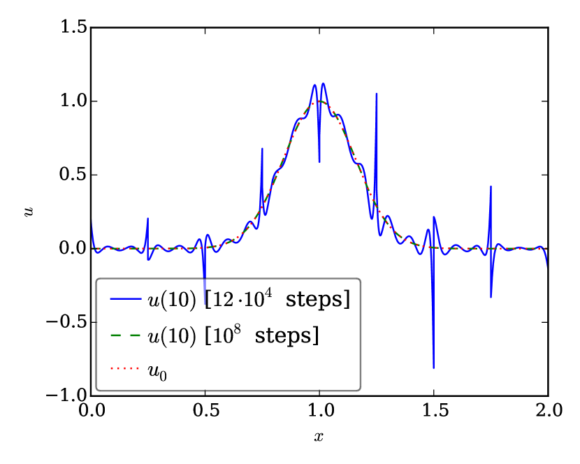
(a) Solution computed without modal filtering.

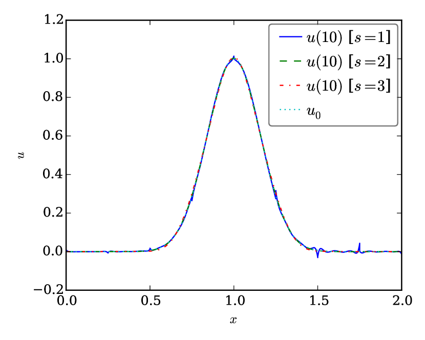
(b) Solution computed using adaptive modal filtering.

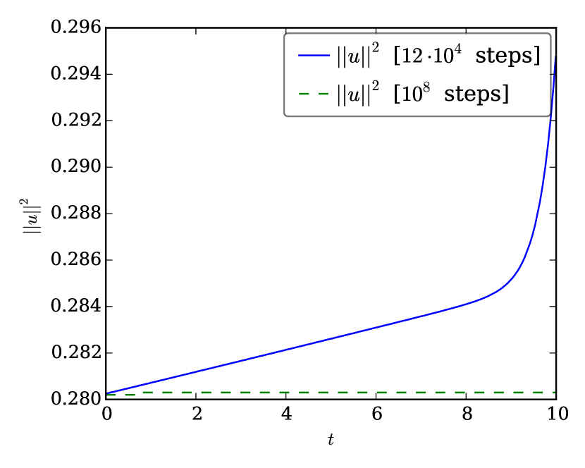
(c) Energy of the solution computed without additional modal filtering.

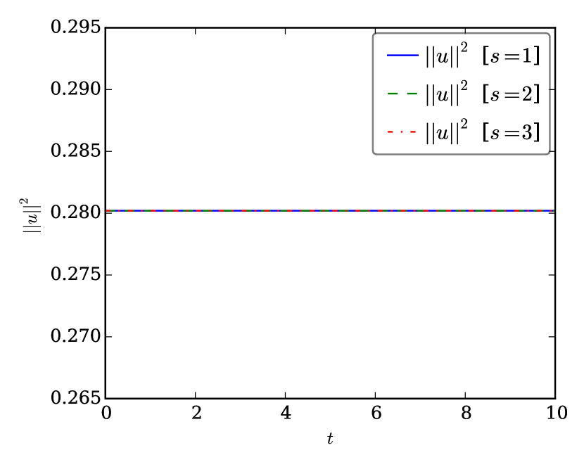
(d) Energy of the solution computed using adaptive modal filtering.

Figure 1: Numerical results for linear advection using $N=8$ elements with polynomials of degree $\leq p=7$. On the left hand side, no modal filtering has been used, whereas adaptive modal filters of orders $s=1$, $s=2$, and $s=3$ have been applied for the right hand side.

Figure 1(a) shows the oscillating solution without modal filtering using $12\cdot 10^{4}$ time steps. The corresponding increasing energy is plotted in Figure 1(c). However, increasing the number of time steps to $10^{6}$ drastically reduces both the increase of energy and the oscillations.

On the other hand, applying modal filters of order $s\in\mathinner{\left\{1,2,3\right\}}$ with adaptively chosen strength $\varepsilon$ according to Lemma 3 results in constant energy in Figure 1(d) and non-oscillatory solutions in Figure 1(b). Only the numerical solution computed with filters of order $s=1$ shows slight peaks in the smooth part.

(a) Solutions for order $s=1$.

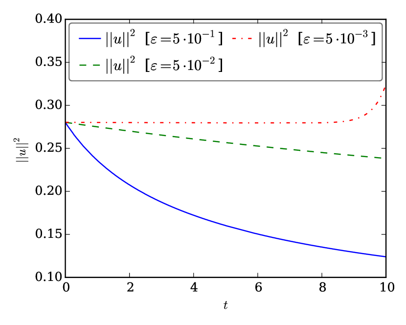
(b) Energies for order $s=1$.

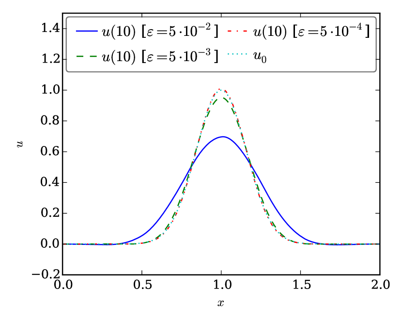
(c) Solutions for order $s=2$.

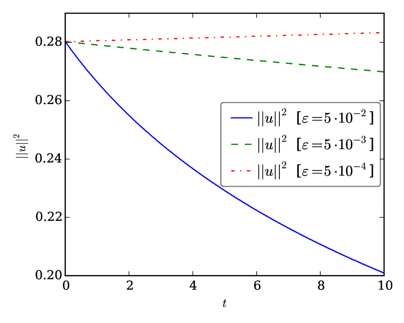
(d) Energies for order $s=2$.

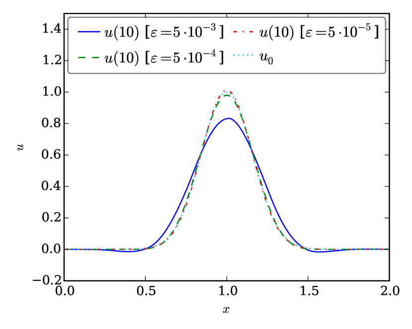
(e) Solutions for order $s=3$.

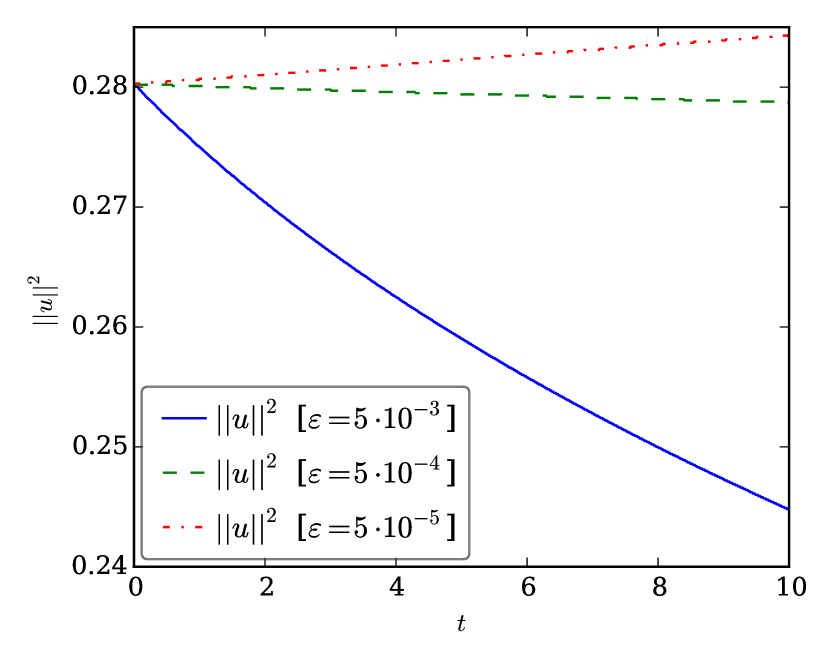
(f) Energies for order $s=3$.

Figure 2: Numerical results for linear advection using $N=8$ elements with polynomials of degree $\leq p=7$ and modal filtering of orders $s\in\mathinner{\left\{1,2,3\right\}}$ with various strengths $\varepsilon$. On the left hand side, the solutions $u$ are shown, accompanied by the corresponding energies $\mathinner{\!\left\lVert u\right\rVert}^{2}$ on the right hand side.

A simple application of modal filtering with constant order $s$ and strength $\varepsilon$ has a stabilising effect, as can be seen in Figure 2. The dissipation increases with increasing strength $\varepsilon$ and order $s$, respectively. However, numerous experiments and fine tuning of the parameters by hand is required in order to get acceptable results. Therefore, the adaptive choice proposed in this work is advantageous.

4.2.2 Linear advection with discontinuous solution

The influence of the presence of discontinuities is investigated using the linear advection equation (4)

$$\partial_{t}u+\partial_{x}u=0,\qquad u(0,x)=u_{0}(x)=\begin{cases}1,&x\in[0.5,1],\\ 0,&\text{otherwise},\end{cases}$$ (28)

and a semidiscretisation (5) using nodal Gauß-Legendre bases of degree $\leq p=7$ on $N=8$ elements with an upwind numerical flux $f^{\mathrm{num}}(u_{-},u_{+})=u_{-}$. The domain $[0,2]$ is equipped with periodic boundary conditions and the solution is advanced in time $t\in[0,8]$ by an explicit Euler method.

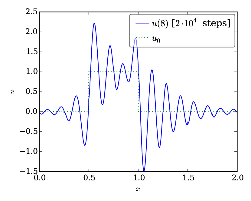
(a) Solution computed without modal filtering.

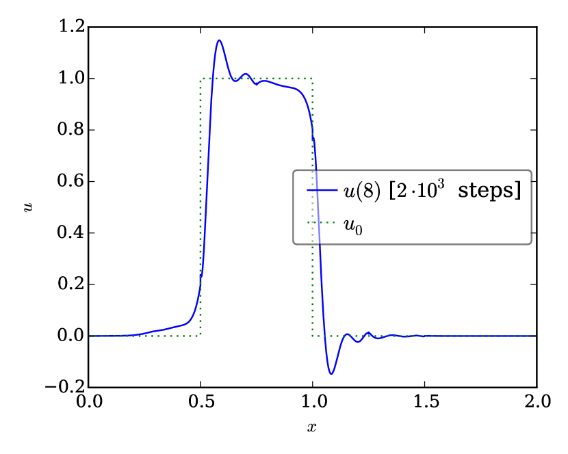
(b) Solution computed using adaptive modal filtering.

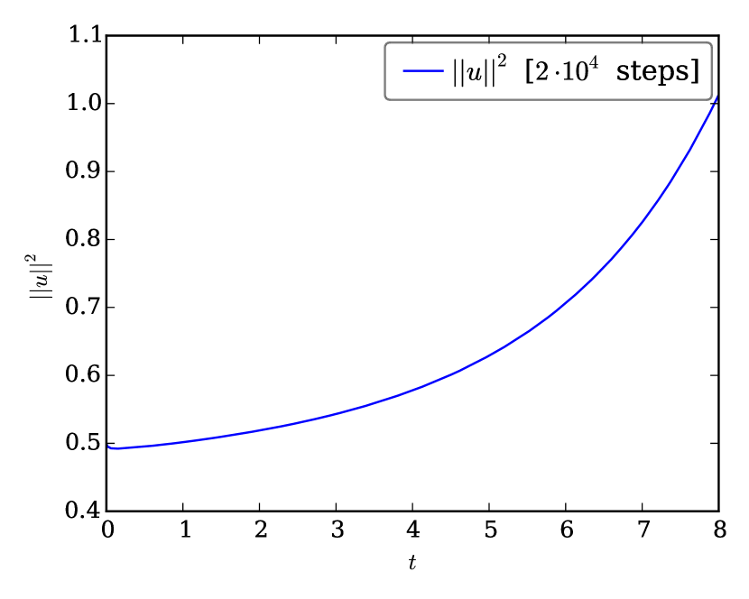
(c) Energy of the solution computed without modal filtering.

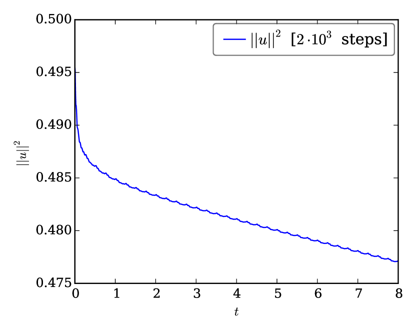
(d) Energy of the solution computed using adaptive modal filtering.

Figure 3: Numerical results for linear advection using $N=16$ elements with polynomials of degree $\leq p=15$. On the left hand side, no modal filtering has been used, whereas adaptive modal filters of order $s=1$ have been used for the right hand side.

Using $2\cdot 10^{4}$ time steps, the solution without modal filtering in Figure 3(a) is oscillatory with increasing energy (Figure 3(c)). However, applying modal filtering with adaptively chosen strength $\varepsilon$ yields a much less oscillatory solution in Figure 3(b) with slightly decreasing energy in Figure 3(d) using only $2\cdot 10^{3}$ time steps.

4.2.3 Burgers’ equation

A nonlinear model problem is given by Burgers’ equation (6)

$$\partial_{t}u+\partial_{x}\frac{u^{2}}{2}=0,\quad u(0,x)=u_{0}(x)=\sin\pi x+0.01$$ (29)

in the domain $[0,2]$ with periodic boundary conditions. The semidiscretisation (7) with $N=16$ elements using Gauß-Legendre bases of degree $\leq p=15$ and a local Lax-Friedrichs numerical flux $f^{\mathrm{num}}(u_{-},u_{+})=\frac{u_{-}^{2}+u_{+}^{2}}{4}-\frac{\max\mathinner{\left\{\mathinner{\!\left\lvert u_{-}\right\rvert},\mathinner{\!\left\lvert u_{+}\right\rvert}\right\}}}{2}(u_{+}-u_{-})$ is applied together with an explicit Euler method.

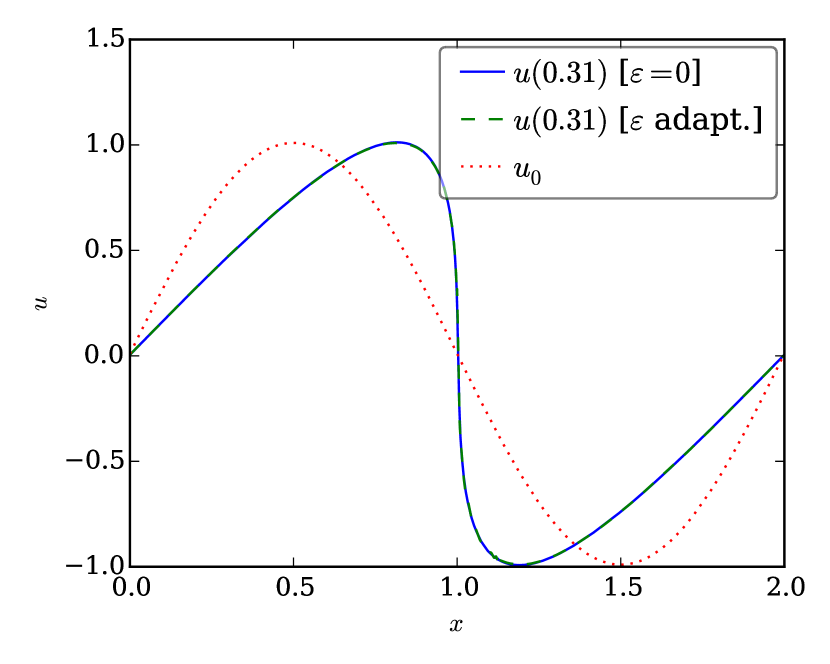
(a) Solution at time $t=0.31$.

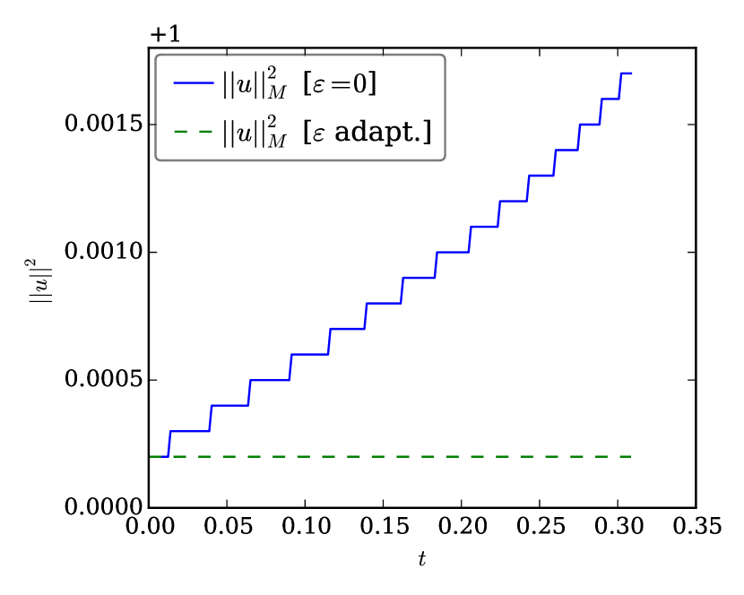
(b) Energy in the time interval $[0,0.31]$.

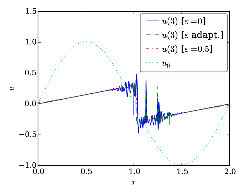
(c) Solution at time $t=3$.

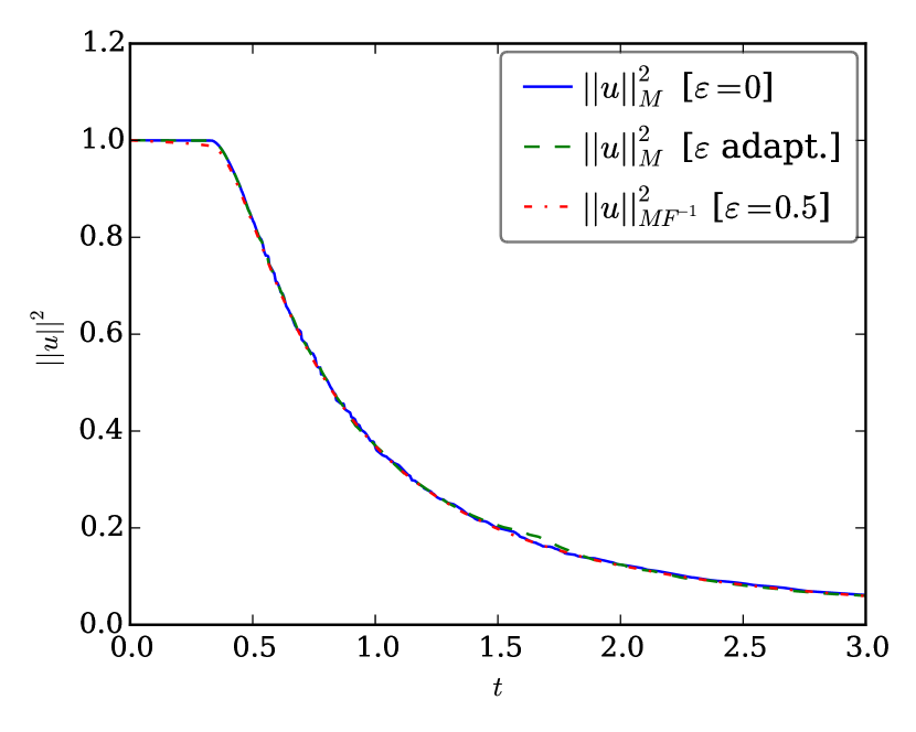
(d) Energy in the time interval $[0,3]$.

Figure 4: Numerical results for Burgers’ equation using $N=16$ elements with polynomials of degree $\leq p=15$. The solutions and the energy are plotted on the left hand side and right hand side, respectively, for the time intervals $[0,0.31]$ (first row) and $[0,3]$ (second row).

The numerical solution up to $t=0.31$ is computed using $200$ time steps and plotted in Figure 4(a) with and without modal filtering. Both solutions coincide visually but the energy increases without modal filtering. However, application of adaptive modal filtering yields a constant energy, as expected.

Contrary, both the solutions and the energy on the complete time interval $[0,3]$ using $15\cdot 10^{3}$ steps are visually indistinguishable, as can be seen in Figures 4(c) and 4(d). Thus, the adaptive modal filtering is not able to remove the oscillations triggered by the developing discontinuity. However, a simple application of a modal filter with fixed strength $\varepsilon=0.5$ results in a non-oscillatory solution.

5 Filtering the time derivative

In this section, possibility 2 of section 3.2 is discussed, i.e. the application of a modal filter $\underline{\underline{F}}\,$ to the time derivative of $\underline{u}$.

5.1 Semidiscrete and discrete estimates

In the following, a conservative and stable semidiscretisation of the scalar conservation law

$$\partial_{t}u+\partial_{x}f(u)=0$$ (30)

relying on elements is assumed, e.g. a CPR method using SBP operators for the linear advection equation with constant speed or Burgers’ equation [19]. This yields on each element an ordinary differential equation

$$\dfrac{\operatorname{d\!}{}}{\operatorname{d\!}{t}}\underline{u}=g(\underline{u}).$$ (31)

Applying the filter $\underline{\underline{F}}\,$ to the time derivative results in

$$\dfrac{\operatorname{d\!}{}}{\operatorname{d\!}{t}}\underline{u}=\underline{\underline{F}}\,g(\underline{u}).$$ (32)

If constant functions are eigenvectors of the filter with eigenvalue $1$, i.e. the filter does not change constants, and the filter is self-adjoint with respect to the mass matrix $\underline{\underline{M}}\,$, i.e. $\underline{\underline{M}}\,\underline{\underline{F}}\,=\underline{\underline{F}}{{}^{T}}\underline{\underline{M}}\,$, then the rate of change of the integral of $\underline{u}$ over an element is

$$\dfrac{\operatorname{d\!}{}}{\operatorname{d\!}{t}}\underline{1}^{T}\underline{\underline{M}}\,\underline{u}=\underline{1}^{T}\underline{\underline{M}}\,\dfrac{\operatorname{d\!}{}}{\operatorname{d\!}{t}}\underline{u}=\underline{1}^{T}\underline{\underline{M}}\,\underline{\underline{F}}\,g(\underline{u})=\underline{1}^{T}\underline{\underline{F}}{{}^{T}}\underline{\underline{M}}\,g(\underline{u})=\underline{1}^{T}\underline{\underline{M}}\,g(\underline{u}),$$ (33)

which is the same as for the semidiscretisation without filtering.

Investigating stability in the norm $\mathinner{\!\left\lVert\cdot\right\rVert}_{M}$ induced by $\underline{\underline{M}}\,$ would start canonically with

$$\frac{1}{2}\dfrac{\operatorname{d\!}{}}{\operatorname{d\!}{t}}\mathinner{\!\left\lVert\underline{u}\right\rVert}_{M}^{2}=\underline{u}^{T}\underline{\underline{M}}\,\dfrac{\operatorname{d\!}{}}{\operatorname{d\!}{t}}\underline{u}=\underline{u}^{T}\underline{\underline{M}}\,\underline{\underline{F}}\,g(\underline{u}).$$ (34)

However, there do not seem to be simple estimates for this rate of change. Contrary, the rate of change of the norm induced by $\underline{\underline{M}}\,\underline{\underline{F}}{{}^{-1}}$ (if $\underline{\underline{F}}\,$ is invertible and $\underline{\underline{M}}\,\underline{\underline{F}}{{}^{-1}}$ induces a scalar product) can be easily estimated as

$$\frac{1}{2}\dfrac{\operatorname{d\!}{}}{\operatorname{d\!}{t}}\mathinner{\!\left\lVert\underline{u}\right\rVert}_{MF^{-1}}^{2}=\underline{u}^{T}\underline{\underline{M}}\,\underline{\underline{F}}{{}^{-1}}\dfrac{\operatorname{d\!}{}}{\operatorname{d\!}{t}}\underline{u}=\underline{u}^{T}\underline{\underline{M}}\,g(\underline{u}),$$ (35)

i.e. the same estimate as for the semidiscretisation without filtering.

Assuming $\underline{\underline{F}}\,$ is invertible, the bilinear form induced by $\underline{\underline{M}}\,\underline{\underline{F}}{{}^{-1}}$ is symmetric iff for all $\underline{v},\underline{u}$

$$\underline{v}^{T}\underline{\underline{M}}\,\underline{\underline{F}}\,\underline{u}=\underline{u}^{T}\underline{\underline{M}}\,\underline{\underline{F}}\,\underline{v},$$ (36)

i.e. $\underline{\underline{F}}\,$ is $\underline{\underline{M}}\,$-self-adjoint $\underline{\underline{M}}\,\underline{\underline{F}}\,=\underline{\underline{F}}{{}^{T}}\underline{\underline{M}}\,$. Assuming $\underline{\underline{M}}\,$ and $\underline{\underline{F}}\,$ are diagonal in a modal Legendre basis with positive entries, then $\underline{\underline{M}}\,\underline{\underline{F}}{{}^{-1}}=\underline{\underline{F}}{{}^{-1/2}}\underline{\underline{M}}\,\underline{\underline{F}}{{}^{-1/2}}$ is positive definite. The modal filters for nodal Gauß- and Lobatto-Legendre as well as modal Legendre bases described in section 3 fulfil these properties.

Lemma 4.

Augmenting a conservative and stable SBP CPR method for the scalar conservation law

$$\partial_{t}u+\partial_{x}f(u)=0$$ (1)

with a modal filter $\underline{\underline{F}}\,$ applied to the time derivative results in a conservative and $\mathinner{\!\left\lVert\cdot\right\rVert}_{MF^{-1}}$-stable semidiscretisation if $\underline{\underline{M}}\,\underline{\underline{F}}{{}^{-1}}$ induces a scalar product. This condition is fulfilled for nodal bases using Gauß- or Lobatto-Legendre points (with lumped mass matrix) and a modal Legendre basis.

This Lemma is connected with the observation of [1], who presented the reformulation of the energy stable CPR methods given by [21] as filtered DG methods, where the filter is applied in the same manner as here. As presented by [19], these CPR methods can conserve the discrete norm induced by some positive definite matrix $\underline{\underline{M}}\,+\underline{\underline{K}}\,$, corresponding to $\underline{\underline{M}}\,\underline{\underline{F}}{{}^{-1}}$ in this setting. However, the discrete norm $\mathinner{\!\left\lVert\cdot\right\rVert}_{M}$ oscillates if the norm $\mathinner{\!\left\lVert\cdot\right\rVert}_{M+K}$ is conserved or even dissipated. Thus, the same behaviour can be expected here, if the time discretisation is sufficiently accurate.

However, considering the explicit Euler method as time discretisation, the norm after one time step can be written as

$$\mathinner{\!\left\lVert\underline{u}_{+}\right\rVert}_{M}^{2}=\mathinner{\!\left\lVert\underline{u}+\Delta t\partial_{t}\underline{u}\right\rVert}_{M}^{2}=\mathinner{\!\left\lVert\underline{u}\right\rVert}_{M}^{2}+2\Delta t\left\langle u,\partial_{t}u\right\rangle_{M}+(\Delta t)^{2}\mathinner{\!\left\lVert\partial_{t}\underline{u}\right\rVert}_{M}^{2}.$$ (37)

Thus, there is an additional increment of the norm not considered in the semidiscrete setting of order $(\Delta t)^{2}$, since the second term is estimated for semidiscretisations. Applying a filter $\underline{\underline{F}}\,$ to the time derivative yields

$$\mathinner{\!\left\lVert\underline{u}_{+}\right\rVert}_{MF^{-1}}^{2} =\mathinner{\!\left\lVert\underline{u}+\Delta t\underline{\underline{F}}\,\partial_{t}\underline{u}\right\rVert}_{MF^{-1}}^{2}$$ (38)

$$=\mathinner{\!\left\lVert\underline{u}\right\rVert}_{MF^{-1}}^{2}+2\Delta t\left\langle u,\underline{\underline{F}}\,\partial_{t}u\right\rangle_{MF^{-1}}+(\Delta t)^{2}\mathinner{\!\left\lVert\underline{\underline{F}}\,\partial_{t}\underline{u}\right\rVert}_{MF^{-1}}^{2},$$

which can be rewritten using $\underline{\underline{F}}{{}^{T}}\underline{\underline{M}}\,=\sqrt{\underline{\underline{F}}{{}^{T}}}\underline{\underline{M}}\,\sqrt{\underline{\underline{F}}\,}$ as

$$\mathinner{\!\left\lVert\underline{u}_{+}\right\rVert}_{MF^{-1}}^{2}=\mathinner{\!\left\lVert\underline{u}\right\rVert}_{MF^{-1}}^{2}+2\Delta t\left\langle u,\partial_{t}u\right\rangle_{M}+(\Delta t)^{2}\mathinner{\!\left\lVert\underline{\underline{F}}{{}^{1/2}}\partial_{t}\underline{u}\right\rVert}_{M}^{2}.$$ (39)

Thus, if the filter $\underline{\underline{F}}\,$ reduces the $\underline{\underline{M}}\,$-norm, the additional increment is smaller then in the case of the unfiltered semidiscretisation. By equivalence of discrete norms, a reduced increase of the norm $\mathinner{\!\left\lVert\cdot\right\rVert}_{M}$ can be expected.

5.2 Numerical experiments

The linear advection equation with discontinuous initial data (28) is solved numerically by an SBP CPR semidiscretisation using $N=8$ elements with Gauß-Legendre bases of degree $\leq p=7$ and an upwind numerical flux $f^{\mathrm{num}}(u_{-},u_{+})=u_{-}$. The solution on the domain $[0,2]$ with periodic boundary conditions is advanced in time $t\in[0,8]$ by an explicit Euler method using $10^{5}$ steps.

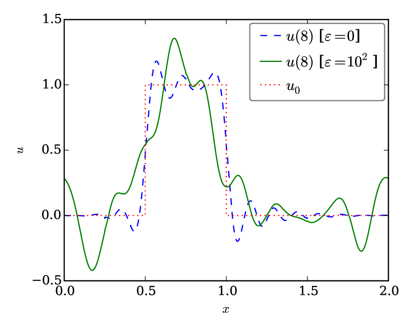
(a) Solution.

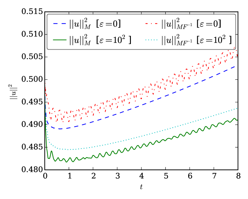
(b) Energy.

Figure 5: Numerical results for linear advection using $N=8$ elements with polynomials of degree $\leq p=7$ with and without modal filtering of the time derivative.

Figure 5(a) shows the solution after $10^{5}$ time steps with and without modal filtering of the time derivative, i.e. for $\varepsilon\in\mathinner{\left\{0,100\right\}}$. It is obvious that the filter did not reduce the oscillations. Contrary, these were intensified.

The time development of the norms are plotted in Figure 5(b). At first, the norm $\mathinner{\!\left\lVert u\right\rVert}_{M}$ decreases without filtering. Starting at $t\approx 1$, it increases monotonically. The corresponding norm $\mathinner{\!\left\lVert u\right\rVert}_{MF^{-1}}$ follows the same trend, but is highly oscillatory. Contrary, the norm $\mathinner{\!\left\lVert u\right\rVert}_{MF^{-1}}$ is smoothly de- and increasing if a modal filter of strength $\varepsilon=100$ is applied to the time derivative and the corresponding norm $\mathinner{\!\left\lVert u\right\rVert}_{M}$ is oscillatory, as expected.

6 Filtering the solution

Here, possibility 3 of section 3.2 is investigated, i.e. the application of a modal filter $\underline{\underline{F}}\,$ to the function $\underline{u}$, used to compute the time derivative.

6.1 Discrete estimates

Using again a conservative and stable semidiscretisation of the scalar conservation law

$$\partial_{t}u+\partial_{x}f(u)=0$$ (1)

as in section 5 results on each element in an ordinary differential equation

$$\dfrac{\operatorname{d\!}{}}{\operatorname{d\!}{t}}\underline{u}=g(\underline{u}).$$ (40)

Now, a modal filter is applied to the function used to compute the time derivative, i.e. $\partial_{t}\underline{u}\mapsto\partial_{t}\underline{\underline{F}}\,\underline{u}$ and the ODE becomes

$$\dfrac{\operatorname{d\!}{}}{\operatorname{d\!}{t}}\underline{u}=g(\underline{\underline{F}}\,\underline{u}).$$ (41)

Using an explicit Euler method as time discretisation, the value after one time step of size $\Delta t$ can be written as

$$\underline{u}_{+}=\underline{u}+\Delta t\,\partial_{t}\underline{\underline{F}}\,\underline{u}.$$ (42)

If the filter $\underline{\underline{F}}\,$ is invertible, this can be rewritten as

$$\underline{u}_{+}=\underline{\underline{F}}{{}^{-1}}\left(\underline{\underline{F}}\,\underline{u}+\Delta t\,\underline{\underline{F}}\,\partial_{t}\underline{\underline{F}}\,\underline{u}\right).$$ (43)

The term in brackets corresponds to a discrete combination of the approaches 1 and 2 mentioned in section 3.2: At first, the filter $\underline{\underline{F}}\,$ is applied in a split operator fashion to the solution $\underline{u}$ and afterwards a time step using a scheme with filter $\underline{\underline{F}}\,$ applied to the time derivative is used.

If the assumptions of the previous sections are complied with, the second step corresponds to a stable semidiscretisation with respect to the norm induced by $\underline{\underline{M}}\,\underline{\underline{F}}{{}^{-1}}$. The additional application of a filter prior to this step could control the additional terms similarly to the way described in section 4.

However, after a full time step of this split operator formulation with filtered time derivative, the inverse filter $\underline{\underline{F}}{{}^{-1}}$ is applied, destroying this stability estimates. Therefore, we do not expect this scheme to be superior compared to the other possibilities mentioned in section 3.2.

6.2 Numerical experiments

The same setup as in the previous section 5.2 is used to compute numerical solutions of the linear advection equation with discontinuous initial data (28).

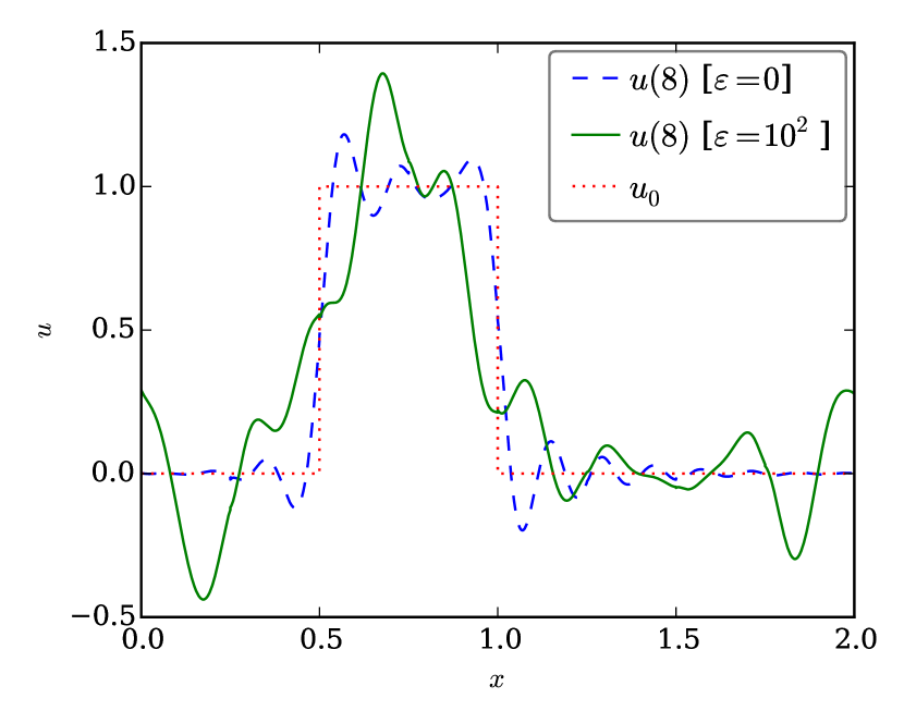
(a) Solution.

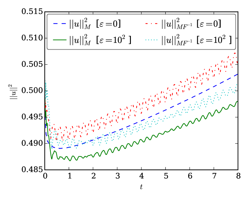
(b) Energy.

Figure 6: Numerical results for linear advection using $N=8$ elements with polynomials of degree $\leq p=7$ with and without modal filtering of the solution.

The solution in Figure 6(a) is very similar to the one in Figure 5(a) of the previous section, as could be guessed from equation (43), if the first application of the filter $\underline{\underline{F}}\,$ and the inverse filter $\underline{\underline{F}}{{}^{-1}}$ are ignored. Especially, the application of modal filtering in this setting does not decrease oscillations or increase the quality of the solution.

However, the influence of the additional terms in equation (43) become visible in the energy of the numerical solution in Figure 6(b). The norms without application of modal filtering are the same as in Figure 5(b) of the previous section, whereas the norms $\mathinner{\!\left\lVert u\right\rVert}_{M}$ and $\mathinner{\!\left\lVert u\right\rVert}_{MF^{-1}}$ of the filtered solution are both oscillating.

7 Conclusions and further research

In this work, modal filtering has been applied in the general framework of CPR methods using SBP operators. It is shown to be equivalent to the application of artificial dissipation / spectral viscosity up to first order in time and circumvents the time step restrictions of these schemes described in the first part of this series by [17].

Additionally, a new adaptive method to chose the filter strength automatically has been proposed. Compensating error terms of order $(\Delta t)^{2}$, the fully discrete schemes using an explicit Euler method become provably stable. However, this adaptive filtering does not remove all oscillations of the numerical solutions, especially in the nonlinear case developing discontinuities.

Moreover, two other possibilities of the application of modal filtering are investigated. Theoretical considerations about their inferior stability properties are accompanied by numerical experiments verifying these.

However, the analysis has been limited to the explicit Euler method as time discretisation. Although these results carry over to strong-stability preserving methods composed of explicit Euler steps, specialised investigations will be conducted.

Of course, an extension of these results to other hyperbolic conservation laws will be interesting.

References

- [1] Y Allaneau and Antony Jameson “Connections between the filtered discontinuous Galerkin method and the flux reconstruction approach to high order discretizations” In Computer Methods in Applied Mechanics and Engineering 200.49 Elsevier, 2011, pp. 3628–3636
- [2] David C Del Rey Fernández, Jason E Hicken and David W Zingg “Review of summation-by-parts operators with simultaneous approximation terms for the numerical solution of partial differential equations” In Computers & Fluids 95 Elsevier, 2014, pp. 171–196
- [3] Jan Glaubitz, Philipp Öffner and Thomas Sonar “Application of Modal Filtering to a Spectral Difference Method” Submitted, 2016 arXiv:1604.00929 [math.NA]
- [4] Sigal Gottlieb, David I Ketcheson and Chi-Wang Shu “Strong stability preserving Runge-Kutta and multistep time discretizations” World Scientific, 2011
- [5] Sigal Gottlieb and Chi-Wang Shu “Total variation diminishing Runge-Kutta schemes” In Mathematics of Computation 67.221, 1998, pp. 73–85
- [6] Jan Hesthaven and Robert Kirby “Filtering in Legendre spectral methods” In Mathematics of Computation 77.263, 2008, pp. 1425–1452
- [7] David I Ketcheson “Highly efficient strong stability-preserving Runge-Kutta methods with low-storage implementations” In SIAM Journal on Scientific Computing 30.4 SIAM, 2008, pp. 2113–2136
- [8] Peter D Lax “Hyperbolic systems of conservation laws and the mathematical theory of shock waves” SIAM, 1973
- [9] Heping Ma “Chebyshev–Legendre Spectral Viscosity Method for Nonlinear Conservation Laws” In SIAM Journal on Numerical Analysis 35.3 SIAM, 1998, pp. 869–892
- [10] Heping Ma “Chebyshev–Legendre Super Spectral Viscosity Method for Nonlinear Conservation Laws” In SIAM Journal on Numerical Analysis 35.3 SIAM, 1998, pp. 893–908
- [11] Yvon Maday and Eitan Tadmor “Analysis of the spectral vanishing viscosity method for periodic conservation laws” In SIAM Journal on Numerical Analysis 26.4 SIAM, 1989, pp. 854–870
- [12] Ken Mattsson, Magnus Svärd and Jan Nordström “Stable and accurate artificial dissipation” In Journal of Scientific Computing 21.1 Springer, 2004, pp. 57–79
- [13] Andreas Meister, Sigrun Ortleb and Thomas Sonar “Application of spectral filtering to discontinuous Galerkin methods on triangulations” In Numerical Methods for Partial Differential Equations 28.6 Wiley Online Library, 2012, pp. 1840–1868
- [14] Andreas Meister, Sigrun Ortleb, Thomas Sonar and Martina Wirz “An extended discontinuous Galerkin and spectral difference method with modal filtering” In ZAMM-Journal of Applied Mathematics and Mechanics/Zeitschrift für Angewandte Mathematik und Mechanik 93.6-7 Wiley Online Library, 2013, pp. 459–464
- [15] Jan Nordström “Conservative finite difference formulations, variable coefficients, energy estimates and artificial dissipation” In Journal of Scientific Computing 29.3 Springer, 2006, pp. 375–404
- [16] Jan Nordström and Peter Eliasson “New developments for increased performance of the SBP-SAT finite difference technique” In IDIHOM: Industrialization of High-Order Methods-A Top-Down Approach Springer, 2015, pp. 467–488
- [17] Hendrik Ranocha, Jan Glaubitz, Philipp Öffner and Thomas Sonar “Enhancing stability of correction procedure via reconstruction using summation-by-parts operators I: Artificial dissipation” Submitted, 2016
- [18] Hendrik Ranocha, Philipp Öffner and Thomas Sonar “Extended skew-symmetric form for summation-by-parts operators” Submitted, 2015 arXiv:1511.08408 [math.NA]
- [19] Hendrik Ranocha, Philipp Öffner and Thomas Sonar “Summation-by-parts operators for correction procedure via reconstruction” In Journal of Computational Physics 311 Elsevier, 2016, pp. 299–328 DOI: 10.1016/j.jcp.2016.02.009
- [20] Magnus Svärd and Jan Nordström “Review of summation-by-parts schemes for initial-boundary-value problems” In Journal of Computational Physics 268 Elsevier, 2014, pp. 17–38
- [21] Peter E Vincent, Patrice Castonguay and Antony Jameson “A new class of high-order energy stable flux reconstruction schemes” In Journal of Scientific Computing 47.1 Springer, 2011, pp. 50–72