HATS-18b: An Extreme Short–Period Massive Transiting Planet Spinning Up Its Star

Abstract

We report the discovery by the HATSouth network of HATS-18b: a $1.980\pm 0.077$ $M_{\rm J}$, $1.337_{-0.049}^{+0.102}$ $R_{\rm J}$ planet in a $0.8378$ day orbit, around a solar analog star (mass $1.037\pm 0.047$ $M_{\sun}$, and radius $1.020_{-0.031}^{+0.057}$ $R_{\sun}$) with $V=14.067\pm 0.040$ mag. The high planet mass, combined with its short orbital period, implies strong tidal coupling between the planetary orbit and the star. In fact, given its inferred age, HATS-18 shows evidence of significant tidal spin up, which together with WASP-19 (a very similar system) allows us to constrain the tidal quality factor for Sun–like stars to be in the range $6.5\lesssim\log_{10}(Q^{*}/k_{2})\lesssim 7$ even after allowing for extremely pessimistic model uncertainties. In addition, the HATS-18 system is among the best systems (and often the best system) for testing a multitude of star–planet interactions, be they gravitational, magnetic or radiative, as well as planet formation and migration theories.

1. Introduction

Hot Jupiters, gas giant planets with orbital periods shorter than a few days, are among the easiest extrasolar planets to detect through either transit or radial velocity (RV) searches (to date, the two most productive methods). In spite of that, the sample of these planets is rather small, showing that they are intrinsically rare. Among those, giant planets with extreme short-period orbits, say under one day, are the easiest to detect yet the most scarce. In fact, out of the 4696 candidate planet Kepler objects of interest (KOI) on the NASA exoplanet archive, only 229 have a radius of at least 6 Earth radii (approximately half the radius of Jupiter) and orbital periods shorter than 5 days, and of those, only 41 have a periods shorter than 1 day. This, combined with the fact, that these are expected to be the KOIs with the highest chance of being false positives (c.f. Fressin et al., 2013), have the highest probability to transit and that none of the transiting ones should be missed by Kepler, demonstrates how unusual these planetary systems are.

On the other hand, this exotic population of planets, especially the ones transiting their star, is very valuable, since it pushes theories of planet formation, structure and evolution, as well as planet–star interactions to the limit (c.f. Ida & Lin, 2008; Dawson & Murray-Clay, 2013; Albrecht et al., 2012; Ginzburg & Sari, 2015; Penev et al., 2012). In addition, the deep and frequent transits and large RV signals of these objects make them the easiest to carry follow–up studies on, thus enhancing their power to constrain theories even further.

We report the discovery by the HATSouth transit survey (Bakos et al., 2013) of HATS-18b: a very short period ($0.8378$ day) massive ($1.980\pm 0.077$ $M_{\rm J}$) extrasolar planet around a star very similar to our Sun (mass $1.037\pm 0.047$ $M_{\sun}$, radius $1.020_{-0.031}^{+0.057}$ $R_{\sun}$ and effective temperature $5600\pm 120$ K). Due to the proximity of the planet to its host star, this system provides one of the best laboratories for testing theories of star–planet interactions and planet formation. In fact, we argue that HATS-18 shows signs of being tidally spun–up by the planet, and that modelling this effect for this system alone constrains the tidal dissipation efficiency of the host star to better than an order of magnitude even with very generous assumptions on possible formation scenarios or model parameter uncertainties. Further, we show that expanding such models to the few other very short period systems, should drastically improve that constraint. Further, such modelling may begin to disentangle some of the very poorly understood physics behind tidal dissipation by measuring its dependence on various system properties.

The layout of the paper is as follows: in § 2 we describe the discovery and follow–up observations used to confirm HATS-18b as a planet; in § 3 we outline the combined photometric and spectroscopic analysis performed and give the inferred system properties; in § 4 we place HATS-18 in the context of other extremely short period exoplanet systems; in § 5 we derive constraints on the tidal quality factor for stars similar to the Sun by modelling HATS-18 and WASP-19’s orbital and stellar spin evolution; and we conclude with a discussion in § 6.

2. Observations

2.1. Photometry

2.1.1 Photometric detection

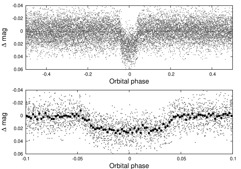
The star HATS-18 (Table 3) was observed by HATSouth instruments between UT 2011 April 18 and UT 2013 July 21 using the HS-2, HS-4, and HS-6 units at the Las Campanas Observatory in Chile, the High Energy Spectroscopic Survey site in Namibia, and Siding Spring Observatory in Australia, respectively. A total of 5372, 3758 and 4008 images of HATS-18 were obtained with HS-2, HS-4 and HS-6, respectively. The observations were obtained through a Sloan $r$ filter with an exposure time of 240 s. The data were reduced to trend-filtered light curves using the aperture photometry pipeline described by Penev et al. (2013) and making use of External Parameter Decorrelation (EPD; Bakos et al., 2010) and the Trend Filtering Algorithm (TFA; Kovács et al., 2005) to remove systematic variations. We searched for transits using the Box Least Squares (BLS; Kovács et al., 2002) algorithm, and detected a $P=0.8378{}$ day periodic transit signal in the light curve of HATS-18 (Figure 1; the data are available in Table 2.1.2). After detecting the signal we re-applied the TFA filter, this time in signal reconstruction mode, so as to obtain an undistorted trend-filtered light curve. The per–point root mean square (RMS) residual combined filtered HATSouth light curve (after subtracting the best-fit model transit) is 0.015 mag, which is typical for a star of this magnitude.

Figure 1.— Unbinned instrumental $r$ band light curve of HATS-18 folded with the period $P=0.8378434$ days resulting from the global fit described in Section 3. The solid line shows the best-fit transit model (see Section 3). In the lower panel we zoom–in on the transit; the dark filled points here show the light curve binned in phase using a bin-size of 0.002.

2.1.2 Photometric follow-up

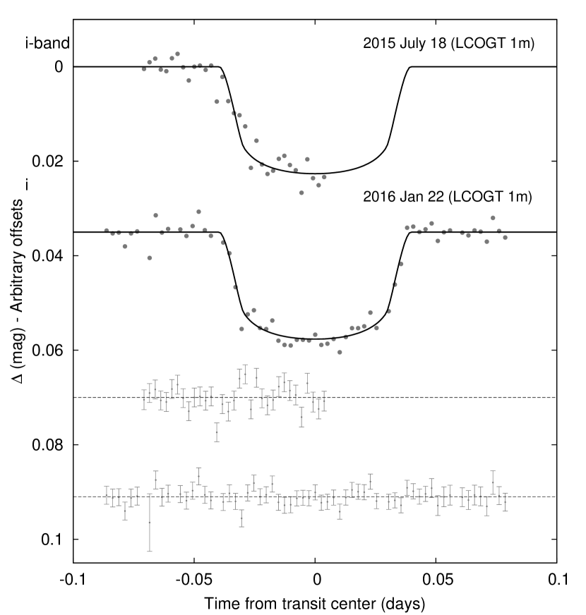
We obtained follow-up light curves of HATS-18 using the LCOGT 1 m telescope network. An ingress was observed on UT 2015 July 18 with the SBIG camera and a Sloan $i$ filter on the 1 m at the South African Astronomical Observatory (SAAO). A total of 33 images were collected at a median cadence of 201 s. A full transit was observed on UT 2016 Jan 22 with the sinistro camera and a Sloan $i$ filter on the 1 m at Cerro Tololo Inter-American Observatory (CTIO). A total of 61 images were collected at a median cadence of 219 s. For the record we also note that a full transit was observed on UT 2016 January 3 with the SBIG camera on the 1 m at SAAO, however due to tracking and weather problems we were unable to extract high precision photometry from these images, and therefore do not include these data in our analysis. For details of the reduction procedure used to extract light curves from the raw images see Penev et al. (2013). The follow-up light curves are shown, together with our best-fit model, in Figure 2, while the data are available in Table 2.1.2. The per-point precision of the SBIG observations is 2.5 mmag, while the per-point precision of the sinistro observations is 1.7 mmag.

Figure 2.— Unbinned follow-up transit light curve of HATS-18 obtained with telescopes from the LCOGT 1 m network. Our best fit is shown by the solid lines. The residuals from the best-fit model are shown below in the same order.

Table 1Differential photometry of HATS-18

BJD	Mag	$\sigma_{\rm Mag}$	Mag(orig)	Filter	Instrument
(2 400 000$+$)
$56442.67216$	$0.03291$	$0.00789$	$\cdots$	$r$	HS
$56411.67208$	$-0.01713$	$0.00723$	$\cdots$	$r$	HS
$56343.80691$	$-0.00841$	$0.00655$	$\cdots$	$r$	HS
$56444.34817$	$0.01720$	$0.00712$	$\cdots$	$r$	HS
$56392.40213$	$-0.00247$	$0.00646$	$\cdots$	$r$	HS
$56395.75361$	$0.02231$	$0.00737$	$\cdots$	$r$	HS
$56416.69970$	$-0.02166$	$0.00680$	$\cdots$	$r$	HS
$56469.48392$	$-0.02100$	$0.00717$	$\cdots$	$r$	HS
$56446.86219$	$-0.00054$	$0.00641$	$\cdots$	$r$	HS
$56458.59202$	$-0.03131$	$0.00744$	$\cdots$	$r$	HS

[-1.5ex]

Note. — This table is available in a machine-readable form in the online journal. A portion is shown here for guidance regarding its form and content. The data are also available on the HATSouth website at http://www.hatsouth.org.

2.2. Spectroscopy

Spectroscopic follow-up observations of HATS-18 were carried out with WiFeS on the ANU 2.3 m telescope (Dopita et al., 2007) and with FEROS on the MPG 2.2 m (Kaufer & Pasquini, 1998).

A total of three spectra were obtained with WiFeS between UT 2015 Feb 28 and UT 2015 Mar 2, two at a resolution of $R\equiv\Delta\,\lambda\,/\,\lambda=7000$, and one at $R=3000$. These data were reduced and analyzed following the procedure described by Bayliss et al. (2013). The $R=3000$ spectrum was used to estimate the spectral type and surface gravity of HATS-18 (we find that it is a G dwarf), while the $R=7000$ spectra were used to rule out an RV variation greater than 5 $\rm km\,s^{-1}$.

We obtained six $R=48000$ spectra with FEROS between UT 2015 Jun 12 and UT 2015 Jun 20. These were reduced to high precision RV and spectral line bisector span (BS) measurements following Jordán et al. (2014), and were also used to determine high precision atmospheric parameters (Section 3). The RVs show a clear $K=415.2\pm 10.0{}$ $\rm m\,s^{-1}$ sinusoidal variation in phase with the transit ephemeris (Figure 3; the data are provided in Table 2.2), confirming this object as a transiting planet system. The BSs exhibit significant scatter, as is typical for a faint $V=14.067\pm 0.040$ mag star, but are uncorrelated with the RVs. The scatter is also well below the level expected if this were a blended stellar eclipsing binary system (Section 3).

Figure 3.— Top panel: High-precision RV measurements from MPG 2.2 m/FEROS together with our best-fit orbit model. Zero phase corresponds to the time of mid-transit. The center-of-mass velocity has been subtracted. Second panel: Velocity $O\!-\!C$ residuals from the best-fit model. The error bars include the jitter which is varied in the fit. Third panel: Bisector spans (BS). Note the different vertical scales of the panels.

Table 2 Relative radial velocities and bisector span measurements of HATS-18.

3. Analysis

Figure 4.— Comparison between the measured values of $T_{\rm eff\star}$ and $\rho_{\star}$ (from ZASPE applied to the FEROS spectra, and from our modeling of the light curves and RV data, respectively), and the Y² model isochrones from Yi et al. (2001). The best-fit values (dark filled circle), and approximate 1$\sigma$ and 2$\sigma$ confidence ellipsoids are shown. The values from our initial ZASPE iteration are shown with the open triangle. The Y² isochrones are shown for ages of 0.2 Gyr, and 1.0 to 14.0 Gyr in 1 Gyr increments.

We analyzed the photometric and spectroscopic observations of HATS-18 to determine the parameters of the system using the standard procedures developed for HATNet and HATSouth (see Bakos et al., 2010, with modifications described by Hartman et al., 2012).

High-precision stellar atmospheric parameters were measured from the FEROS spectra using ZASPE (Brahm et. al., 2016). The resulting $T_{\rm eff\star}$ and $\rm[Fe/H]$ measurements were combined with the stellar density $\rho_{\star}$ determined through our joint light curve and RV curve analysis, to determine the stellar mass, radius, age, luminosity, and other physical parameters, by comparison with the Yonsei-Yale (Y²; Yi et al., 2001) stellar evolution models (see Figure 4). This provided a revised estimate of $\log{g_{\star}}$ which was fixed in a second iteration of ZASPE. Our final adopted stellar parameters are listed in Table 3. We find that the star HATS-18 has a mass of $1.037\pm 0.047$ $M_{\sun}$, a radius of $1.020_{-0.031}^{+0.057}$ $R_{\sun}$, and is at a reddening-corrected distance of $645_{-25}^{+36}$ pc.

We simultaneously carried out a joint analysis of the High-precision FEROS RVs (fit using a Keplerian orbit) and the HS and LCOGT 1 m light curves (fit using a Mandel & Agol, 2002 transit model with fixed quadratic limb darkening coefficients taken from Claret, 2004) to measure the stellar density, as well as the orbital and planetary parameters. This analysis makes use of a differential evolution Markov Chain Monte Carlo procedure (DEMCMC; ter Braak, 2006) to estimate the posterior parameter distributions, which we use to determine the median parameter values and their 1$\sigma$ uncertainties. The results are listed in Table 4. We find that the planet HATS-18b has a mass of $1.980\pm 0.077$ $M_{\rm J}$, and a radius of $1.337_{-0.049}^{+0.102}$ $R_{\rm J}$. We fit the data both assuming a circular orbit, and allowing for a non-zero eccentricity. We find that the observations are consistent with a circular orbit: $e=0.063\pm 0.049$, with a 95% confidence upper-limit of $e<0.166{}$, and therefore adopt the parameters that come from assuming a circular orbit (we also find that the Bayesian evidence for the circular orbit model is higher than the evidence for the free-eccentricity model).

3.1. Ruling Out Blended Models

In order to rule out the possibility that HATS-18 is a blended stellar eclipsing binary system, we carried out a blend analysis of the photometric data following Hartman et al. (2012). We find that all blend models tested can be rejected based on the photometry alone with $3.5\sigma$ confidence. Moreover, the blend models which come closest to fitting the photometry (those which cannot be rejected with greater than $5\sigma$ confidence) yield simulated RVs that are not at all similar to what we observe (i.e., the simulated blend-model RVs do not show a sinusoidal variation in phase with the photometric ephemeris). We conclude that HATS-18 is not a blended stellar eclipsing binary system, and is instead a transiting planet system.

3.2. Photometric Rotation Period

Figure 5.— Top: The Lomb–Scargle periodogram of HATS-18 light curves (in signal reconstruction mode for the transits but not the rotational modulation) with transits removed. Bottom: the same lightcurve folded with the best–fit stellar spin period (the points in the second half of the plot are duplicates of those in the first half).

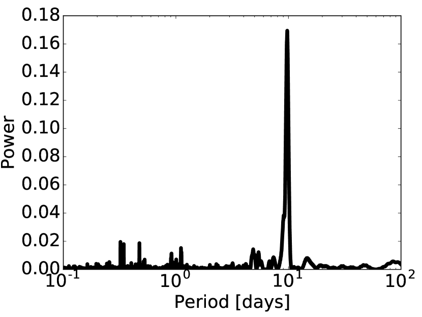
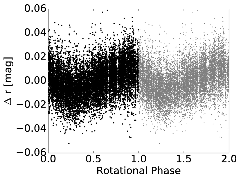
The lightcurve of HATS-18 shows a clear signature of stellar spin variability. In Fig. 5 we show the Lomb–Scargle periodogram of the HATSouth discovery lightcurve of HATS-18, with observations during transits removed, as well as the lightcurve as a function of the best fit spin period (9.8 days) phase. In order to get a handle on the uncertainty in the stellar spin period we split the lightcurve into 9 segments, each containing three spin periods and fit for the rotation period in each segment separately and adopt the standard deviation of the individual measurements as the period uncertainty. The resulting spin period estimate is $P_{rot\star}=9.8\pm 0.4$ days.

Table 3 Stellar Parameters for HATS-18

Parameter	Value	Source
Identifying Information
R.A. (h:m:s)	$11^{\mathrm{h}}35^{\mathrm{m}}49.92{\mathrm{s}}$	2MASS
Dec. (d:m:s)	$-29{\arcdeg}09{\arcmin}21.6{\arcsec}$	2MASS
R.A.p.m. (mas/yr)	$2.7\pm 1.2$	2MASS
Dec.p.m. (mas/yr)	$-4.4\pm 1.2$	2MASS
GSC ID	GSC 6664-00410	GSC
2MASS ID	2MASS 11354977-2909216	2MASS
Spectroscopic properties
$T_{\rm eff\star}$ (K)	$5600\pm 120$	ZASPE
Spectral type	G	ZASPE
$\rm[Fe/H]$	$0.280\pm 0.080$	ZASPE
$v\sin{i}$ ($\rm km\,s^{-1}$)	$6.23\pm 0.47$	ZASPE
$\gamma_{\rm RV}$ ($\rm m\,s^{-1}$)	$7663.3\pm 7.7$	FEROS
Photometric properties
$B$ (mag)	$14.870\pm 0.060$	APASS
$V$ (mag)	$14.067\pm 0.040$	APASS
$g$ (mag)	$14.407\pm 0.020$	APASS
$r$ (mag)	$13.854\pm 0.030$	APASS
$i$ (mag)	$13.77\pm 0.15$	APASS
$J$ (mag)	$12.736\pm 0.026$	2MASS
$H$ (mag)	$12.382\pm 0.028$	2MASS
$K_{s}$ (mag)	$12.289\pm 0.028$	2MASS
Derived properties
$M_{\star}$ ($M_{\sun}$)	$1.037\pm 0.047$	Y2+$\rho_{\star}$+ZASPE
$R_{\star}$ ($R_{\sun}$)	$1.020_{-0.031}^{+0.057}$	Y2+$\rho_{\star}$+ZASPE
$\log{g_{\star}}$ (cgs)	$4.436\pm 0.034$	Y2+$\rho_{\star}$+ZASPE
$\rho_{\star}$ ($\rm g\,cm^{-3}$)	$1.38_{-0.21}^{+0.13}$	Light curves
$\rho_{\star}$ ($\rm g\,cm^{-3}$)	$1.37_{-0.23}^{+0.12}$	Y2+Light curves+ZASPE
$L_{\star}$ ($L_{\sun}$)	$0.93\pm 0.13$	Y2+$\rho_{\star}$+ZASPE
$M_{V}$ (mag)	$4.94\pm 0.17$	Y2+$\rho_{\star}$+ZASPE
$M_{K}$ (mag,ESO)	$3.281\pm 0.099$	Y2+$\rho_{\star}$+ZASPE
Age (Gyr)	$4.2\pm 2.2$	Y2+$\rho_{\star}$+ZASPE
$A_{V}$ (mag)	$0.076_{-0.076}^{+0.114}$	Y2+$\rho_{\star}$+ZASPE
Distance (pc)	$645_{-25}^{+36}$	Y2+$\rho_{\star}$+ZASPE
$P_{rot\star}$ (days)	$9.8\pm 0.4$	HATSouth light curve

Table 4Parameters for the transiting planet HATS-18b.

Parameter	Value
Light curve parameters
$P$ (days)	$0.83784340\pm 0.00000047{}$
$T_{c}$ (${\rm BJD}$)	$2457089.90598\pm 0.00026{}$
$T_{14}$ (days)	$0.07886\pm 0.00083{}$
$T_{12}=T_{34}$ (days)	$0.0101\pm 0.0010{}$
$a/R_{\star}$	$3.71_{-0.22}^{+0.11}{}$
$\zeta/R_{\star}$	$29.09_{-0.19}^{+0.26}{}$
$R_{p}/R_{\star}$	$0.1347\pm 0.0019{}$
$b^{2}$	$0.085_{-0.054}^{+0.110}{}$
$b\equiv a\cos i/R_{\star}$	$0.29_{-0.11}^{+0.15}{}$
$i$ (deg)	$85.5_{-2.8}^{+1.9}{}$
Limb-darkening coefficients
$c_{1},i$ (linear term)	$0.3097{}$
$c_{2},i$ (quadratic term)	$0.3143{}$
$c_{1},r$	$0.4124{}$
$c_{2},r$	$0.2959{}$
RV parameters
$K$ ($\rm m\,s^{-1}$)	$415.2\pm 10.0{}$00
$e$	$<0.166{}$
FEROS RV jitter ($\rm m\,s^{-1}$)	$<11.4$
Planetary parameters
$M_{p}$ ($M_{\rm J}$)	$1.980\pm 0.077{}$
$R_{p}$ ($R_{\rm J}$)	$1.337_{-0.049}^{+0.102}{}$
$C(M_{p},R_{p})$	$0.36{}$
$\rho_{p}$ ($\rm g\,cm^{-3}$)	$1.02_{-0.20}^{+0.13}{}$
$\log g_{p}$ (cgs)	$3.435_{-0.063}^{+0.035}{}$
$a$ (AU)	$0.01761\pm 0.00027{}$
$T_{\rm eq}$ (K)	$2060\pm 59{}$
$\Theta$	$0.0498_{-0.0033}^{+0.0025}{}$
$\langle F\rangle$ ($10^{9}$$\rm erg\,s^{-1}\,cm^{-2}$)	$4.07\pm 0.48{}$

4. Comparison to Other Short Period Systems

Due to its very short orbital period and relatively high planetary mass, the HATS-18 system is ideal for testing theories of star–planet interactions, whether those occur through radiation, gravity or magnetic fields. Figures 6—8 show a comparison between the present sample of giant planets (mass at least $0.1$ $M_{\rm J}$) in orbital periods shorter than two days and the HATS-18 system in a number of parameters related to the strength of various star–planet interactions that have been suggested to occur.

Figure 6.— Size of the planetary orbit relative to the stellar radius as a function of the stellar rotation period, estimated using the measured projected equatorial velocity of the stars and their estimated radii. Planets other than HATS-18(big star symbol) are all transiting planets from the NASA Exoplanet Archive with orbital periods shorter than 2 days and masses at least $0.1$ $M_{\rm J}$. Filled symbols: host star effective temperature is below 6250 K (surface convective zone stars); empty symbols: host star effective temperature is above 6250 K (surface radiative zone stars); half–filled symbols: host star effective temperature is consistent with 6250 K within quoted error bars.

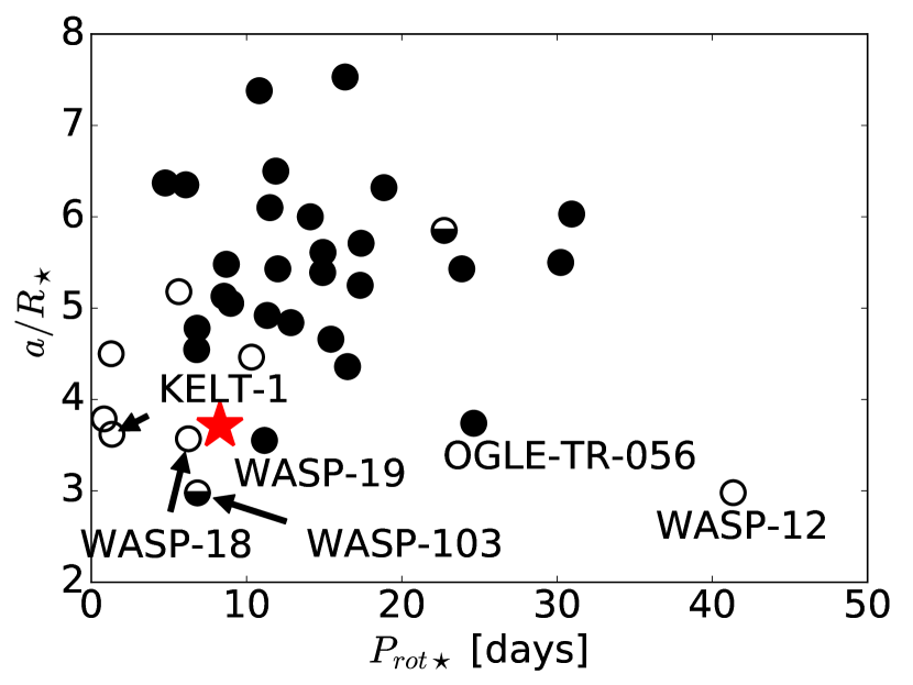
The possible magnetic interactions (and hence their observable effects) are expected to grow in strength the deeper the planet is in its star’s magnetic field and the stronger the field is. In general, stars with surface convective zones are expected to have much stronger magnetic fields than stars with surface radiative zones, since in the former case some form of convectively driven dynamo is expected to operate in the stellar envelope. Further, the dynamo is expected to generate a larger field for faster rotating stars, hence the two readily observable quantities to compare in order to gauge the observability of magnetic star–planet interactions are the size of the orbit relative to the stellar radius ($a/R_{\star}$) and the stellar spin period. From Fig. 6, we see that HATS-18 is among the three surface convective zone systems (HATS-18, WASP-19 and OGLE-TR-56) whose error bars are consistent with having the smallest $a/R_{\star}$  and among those it has the shortest stellar spin period (inferred either from its projected spin velocity, or the observed rotational modulation in its lightcurve).

Figure 7.— The equilibrium temperature of the planet, assuming ideal black body against the fraction of the ratio of the Roche radius to planet radius for the same systems plotted in Fig. 6.

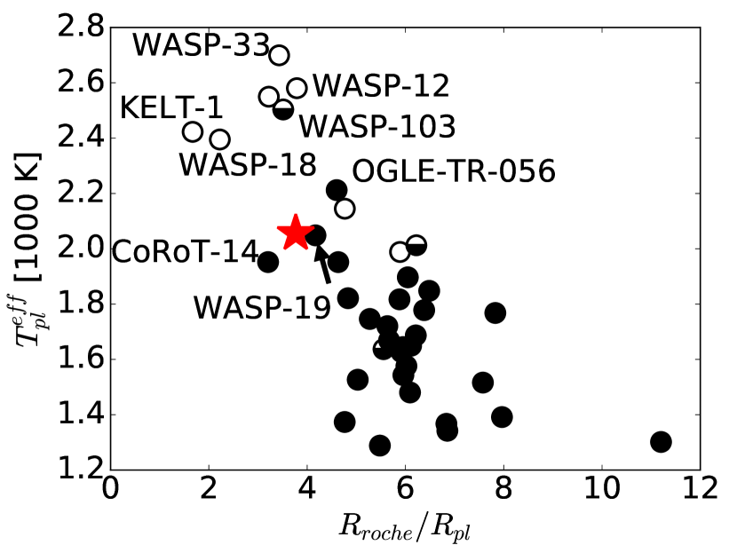
Another rather dramatic effect of star–planet interactions is for the stellar irradiation/wind to drive outflows from the planet. Clearly this process will occur more readily for planets closer to filling their Roche radius and for hotter planets. Fig. 7 plots the ratio of the planetary to the Roche radius for each system against the equilibrium effective temperature for the planet (assuming a perfect black body) for the same sample of planets as in Fig. 6. Again, HATS-18 is among the planets with most favourable parameters, although in this case there is a cluster of very–hot, very small Roche ratio planets around surface radiative zone stars, for one of which (WASP-12b) outflows have been claimed (c.f. Fossati et al., 2010; Haswell et al., 2012).

Figure 8.— The shift in mid–transit time ephemeris after a decade for a tidal quality factor of $Q_{\star}=10^{6}$.

.

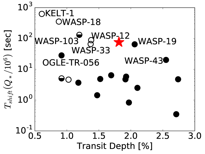
The most direct way of detecting tidal interactions between a star and its companion planet is to see the orbital decay due to tidal dissipation in the star. This is most readily accomplished through observing the resulting deviation from a linear mid–transit time ephemeris. Detecting this effect will provide a direct measurement of the tidal dissipation efficiency of the parent star: the least constrained parameter in tidal interactions involving stars and giant planets. Fig. 8 shows that HATS-18b is the planet around a convective envelope star with the largest expected shift in mid–transit time after a decade.

5. Host Star Spin–Up and a measurement of $Q_{\star}$

Given that HATS-18 has an age consistent with the age of the Sun, and that it is very close to solar mass, its spin period should be close to that of the Sun or to the recently measured rotation periods in the 4.2 Gyr old open cluster M 67 (Barnes et al., 2016): $P_{rot\star}\approx 30$ days, even if the stellar age were at the lower end of the estimated error bar (2.2 Gyrs), the expected spin period is $P_{rot\star}\approx 20$. Instead, in § 3 we found $v\sin{i}$ and stellar radius corresponding to a spin period of $P_{rot\star}=8.3\pm 0.8$ days, which is consistent with the photometrically determined rotation period of $P_{rot\star}=9.8\pm 0.4$ days. This much faster spin rate is close to what is observed for Solar mass stars in clusters with ages around 600 Myr: the 550 Myr old M 37 (Hartman et al., 2009), the 580 Myr old Praesepe (Agüeros et al., 2011; Delorme et al., 2011; Kovács et al., 2014), and the 625 Myr old Hyades (Delorme et al., 2011). A natural explanation for this apparent discrepancy is suggested by the fact that the HATS-18 system contains a very short period giant planet, which should have experienced some orbital decay due to tidal dissipation in the star. The angular momentum taken out of the planetary orbit as it shrinks is deposited in the star and hence the star is spun–up. The fact that we see evidence for this tidal spin–up, means that we can use it to measure the tidal dissipation properties of the star. In this section we describe a method for carrying out such a measurement and show the resulting constraints.

5.1. The Tidal and Stellar Spin Model

Stars like HATS-18 continuously lose angular momentum throughout their lifetime by magnetically imparting angular momentum to the wind of charged particles launched from their surfaces. As a result, in order to relate the stellar tidal dissipation efficiency to the observed stellar spin, we need to model this angular momentum loss simultaneously with the tidal spin–up.

There are a number of options for modelling the tidal evolution, and the angular momentum loss. However, in an effort to keep the number of model parameters small while constructing a consistent model we will use the tidal evolution formulation of (Lai, 2012) and assume a constant value for $Q^{\prime}_{\star}\equiv Q_{\star}/k_{2}$, where $Q_{\star}$ is the fraction of tidal energy lost in one orbital period, and $k_{2}$ is the Love number of the star. Note that, while tidal dissipation in the planet may be more efficient than in the star, it will quickly result in a circular orbit and planetary spin synchronized with the orbit, which will make the tidal deformation of the planet static and hence not subject to dissipation. Further, assuming constant dissipation efficiency is clearly not physical. In particular, the dissipation should vanish ($Q^{\prime}_{\star}=\infty$) when the tidal frequency approaches zero and increase gradually as the frequency moves away from zero. However, for tidal frequencies near that observed for HATS-18, the dissipation is expected to become less efficient as the frequency increases. Since there is currently no agreement on the expected dependence of $Q^{\prime}_{\star}$ on frequency and other parameters, we don’t have a choice but to assume $Q^{\prime}_{\star}=const$. In practice, the way to interpret the results is that the $Q^{\prime}_{\star}$ measured by our analysis is appropriate for the currently observed state of the system analyzed, since the observed spin–up of the host star is overwhelmingly dominated by the very recent tidal evolution (see Fig. 9).

We will model the star as consisting of two distinct zones: the surface convective envelope and the radiative core, and all tidal dissipation will be assumed to occur in the envelope. As a result, any angular momentum lost by the orbit will be deposited exclusively in the convective zone of HATS-18. This will tend to drive differential rotation between the core and the envelope, which will in turn be suppressed by at present not well understood coupling processes, but its efficiency is reasonably constrained by observations (c.f. Irwin et al., 2007; Gallet & Bouvier, 2015; Amard et al., 2016). The model for the evolution of the stellar spin tracks a single value for the spin of each zone, allows for angular momentum exchange between the core and the envelope and for angular momentum loss due to the stellar wind. The particular formulation we will use is given in detail in Irwin et al. (2007).

The loss of angular momentum from the convective envelope due to the wind is given by:

$$\begin{split}\left(\frac{d\vec{J}_{conv}}{dt}\right)_{wind}\equiv&\quad K\vec{\omega}_{conv}\min(\left|\vec{\omega}_{conv}\right|^{2},\omega_{sat}^{2})\\ &\left(\frac{R_{\star}}{R_{\odot}}\right)^{1/2}\left(\frac{M_{\star}}{M_{\odot}}\right)^{-1/2}\end{split}$$ (1)

Where $K$ and $\omega_{sat}$ are parameters for the efficiency of the coupling of the convective zone rotation to the wind, $\vec{J}_{conv}$ is the angular momentum of the convective zone, $\vec{\omega}_{conv}$ is the angular velocity of the convective zone and $\frac{R_{\star}}{R_{\odot}}$ and $\frac{M_{\star}}{M_{\odot}}$ are the radius and mass of the parent star in solar units respectively.

In addition, angular momentum is exchanged between the radiative core and convective envelope by mass exchange and by a torque driving the two zones toward solid body rotation:

$$\begin{split}&\left(\frac{d\vec{J}_{conv}}{dt}\right)_{coup}=-\left(\frac{d\vec{J}_{rad}}{dt}\right)_{coup}=\\ &=\frac{1}{\tau_{c}}\frac{I_{conv}\vec{J}_{rad}-I_{rad}\vec{J}_{conv}}{I_{rad}+I_{conv}}-\frac{2R_{rad}^{2}}{3I_{conv}}\left(\frac{dM_{rad}}{dt}\right)\vec{\omega}_{conv}\end{split}$$ (2)

where $\vec{J}_{rad}$ is the angular momentum of the radiative core, $I_{conv}$ and $I_{rad}$ are the moments of inertia of the convective and radiative zones respectively, $M_{rad}$ and $R_{rad}$ are the mass and outer radius of the radiative zone, and $\tau_{c}$ is a model parameter giving the timescale on which the core and the envelope converge to solid body rotation.

Finally, we will use YREC tracks (Demarque et al., 2008) for the evolution of the stellar quantities ($I_{conv}$, $I_{rad}$, $R_{\star}$, $M_{rad}$ and $R_{rad}$).

The combined orbital and stellar spin evolution described above was computed using a more general version of the POET code (Penev et al., 2014), which, among other things, allows following the evolution for systems in which the stellar spin is misaligned with the orbit.

5.2. Method

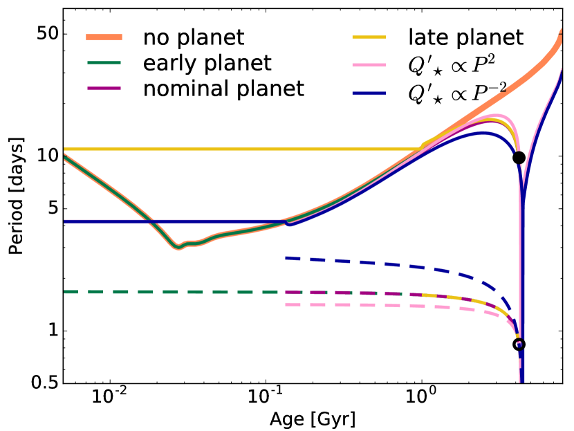
Given values for all model parameters, in order to fully specify the evolution of the system, we need to choose appropriate boundary conditions. Clearly, the observed state of the system provides those, but if we wish to use the observed stellar spin to constrain $Q^{\prime}_{\star}$ we must find independent spin boundary conditions. Fortunately, rotation periods for stars in young open clusters have been widely measured. Conveniently, as long as the stellar spin–down parameters are chosen to reproduce the observed evolution of stellar spin with age in open clusters, it makes very little difference which particular cluster we choose to start the evolution from. This is because for reasonable tidal dissipation rates, only a very tiny fraction of the orbital evolution occurs in the first few hundred Myrs, and as a result, the stellar spin evolution hardly differs from that of an isolated star. This is very fortunate, since our results will not depend on the formation mechanism of HJs. Whether they form very early through disk migration, or much later through high–eccentricity migration, will have only a negligible effect on the final stellar spin. Example evolutions of HATS-18, using the nominal parameters from tables 3 and 4, adding the planet at ages 10 Myrs, 133 Myrs and 1 Gyr are shown in Fig. 9. In all cases, the evolution was started with the spin the star would have if it evolved only under the influence of angular momentum loss to stellar wind, and the initial orbital period of the planet was selected to reproduce the currently observed orbital period at the current age. We can see that, as expected, the effect of the age at which the planet migrates to its short period orbit on the stellar spin is utterly negligible compared to the uncertainty of the measurement. In addition, Fig. 9 also shows that effect of assuming a frequency dependent tidal dissipation is relatively small, with even quite steep dependence on period ($Q^{\prime}_{\star}\propto P^{2}$ or $Q^{\prime}_{\star}\propto P^{-2}$) reproducing the currently observed stellar spin to within 2-sigma of the measured value, as long as $\log_{10}(Q^{\prime}_{\star})=7.3$ at the observed tidal period for HATS-18 (0.46 days).

Figure 9.— Example evolution of HATS-18 spin (solid lines) and HATS-18b orbital period (dashed lines) using the nominal measured parameters for the system and $\log_{10}(Q^{\prime}_{\star})=7.3$ at the observed tidal frequency of 0.46 days. The different lines correspond to adding the planet at ages 10 Myr (early planet), 133 Myrs (nominal planet) and 1 Gyr (late planet) as well as two additional assumptions for the frequency dependence of $Q^{\prime}_{\star}$. The initial orbital period is chosen such that the present orbital period is reproduced at the present age of 4.2 Gyrs (open black circle). The initial stellar spin at the time the planet is added is that of a star evolving only under the influence of angular momentum loss (line labeled no planet) due to stellar wind. Regardless of the assumed planet migration age, the presently observed stellar spin period is reproduced at the present system age (filled black circle), to much better than the measurement uncertainty. The different frequency scaling of $Q^{\prime}_{\star}$ also have a relatively minor effect on the predicted stellar spin (both land within 2-sigma of the measured spin period).

For the constraint derived below, we used the combined spin periods for M 50 (Irwin et al., 2009) and the Pleiades (Hartman et al., 2010), since the two clusters are very close in age, have consistent period distributions, and together provide a large sample of stars for which the spin period has been measured. We assumed a starting age of 133 Myrs for all evolutions, close to the one estimated for the above clusters.

Table 5 The sets of assumptions for which constraints on $\log_{10}(Q^{\prime}_{\star})$ were derived and the results for each system.

In order to constrain the value of the tidal dissipation parameter $Q^{\prime}_{\star}$ defined above, fully accounting for the posterior distributions of the measured HATS-18 system properties, we will follow the following procedure:

1. select a random step from the converged DEMCMC chain, thus getting values for the present age of the HATS-18 system as well as the stellar and planetary masses and the stellar radius.

2. Randomly select one of the stars from the Pleiades/M 50 with measured rotation period that has a mass within $0.1M_{\odot}$ of the randomly selected stellar mass above and use its spin period as the initial spin for the calculated evolution.

3. Select a random value for $log_{10}(Q^{\prime}_{\star})$ from a uniform distribution in the range $(5,9)$.

4. Find an initial orbital period, such that starting the evolution at an age of 133 Myrs with the above parameters and evolving to the randomly selected present system age, results in the observed orbital period (the comparatively tiny uncertainty in the current orbital period is ignored).

5. Assume a normal distribution for the measured stellar spin period at the present age and evaluate the distribution at the resulting stellar spin period with the above evolution to get $p(Q^{\prime}_{\star})$.

Repeating the above steps multiple times allows us to build a cumulative distribution function (CDF) for $log_{10}(Q^{\prime}_{\star})$ by summing up all $p(Q^{\prime}_{\star})$ values up to a particular $log_{10}(Q^{\prime}_{\star})$. The number of iterations was chosen such that doubling their number did not result in significant changes in the CDF.

Finally, the entire procedure was repeated for a number of assumptions about the parameters of the spin model in order to investigate the sensitivity of the constraint to these parameters. In addition, even though planets around stars with surface convective zones appear to be well aligned with their host star’s spin, it is possible that they form with a wide range of obliquities, which then decay on a timescale short compared to the tidal orbital decay for typical planets, but it may not be short compared to the orbital decay for HATS-18. In order to investigate the impact this could have on the results, we also considered the most extreme possible case, of starting the star spinning in exactly the opposite direction to the orbit and evolving to a presently assumed prograde state. The particular set of parameters considered is given in table 5.2. The “nominal” and “retrograde” models use the parameters for the stellar spin evolution which best fit the observed spin periods of open clusters (Irwin et al., 2007). An important point to note is that the change in parameter values away from the nominal model, for the other cases considered, do not represent actual uncertainties. In fact, all of these changes are in dramatic conflict with observations, demonstrating that very large changes in the models are required to make appreciable changes to the inferred $Q^{\prime}_{\star}$ constraint. A more appropriate treatment, which accounts properly for the shifts in the model parameters allowed by the cluster data, is beyond the scope of this paper, but the range of models considered demonstrates the robustness of the results presented here.

In addition to HATS-18, we carried out the steps outlined in the previous section for WASP-19. This is another one of the three planetary systems whose measured semimajor axis to stellar radius ratio is consistent with being the smallest, and hence can be expected to have its host star spun up due to tidal dissipation. Indeed, it also seems to be spinning faster than expected for its age. In fact, Tregloan-Reed et al. (2013) observed the planet transiting in front of, what appears to be the same star spot, on two consecutive nights, which allowed them to measure WASP-19’s spin period to be $11.76\pm 0.09$ days, while the discovery paper (Hebb et al., 2010) quoted a photometrically detected rotation period of $10.5\pm 0.2$ days. Neither of these periods is consistent with the isochronal constraint that the system is older than 1 Gyr (Hebb et al., 2010).

In order to make the results from HATS-18 and WASP-19 as comparable as possible, we used the same set of isochrones and the same fitting procedure to derive an isochronal age for WASP-19 of $8\pm 3$ Gyr. Further, both stars have masses very close to solar, which means we do not need to worry about dependences of the various model parameters on the stellar mass. Finally, a proper DEMCMC fit to the WASP-19 observations is not available, so unlike for HATS-18, we simply assume the relevant parameters for WASP-19 from the literature and use a Normal distribution with the quoted uncertainties. The particular values we employed were taken from Tregloan-Reed et al. (2013), and are consistent with the rest of the literature: $M_{\star}=0.904\pm 0.045M_{\odot}$, $R_{\star}=1.004\pm 0.018R_{\odot}$, $M_{pl}=1.114\pm 0.04M_{J}$, and we adopted the Tregloan-Reed et al. (2013) stellar spin period of $11.76\pm 0.09$ days and orbital period of $P=0.788840\pm 0.0000003$ days.

5.3. Results

Figure 10.— Top: The PDF of $\log_{10}(Q^{\prime}_{\star})$ from the HATS-18 system parameters. The various lines correspond to the models from table 5.2 with the models for which the angular momentum loss parameters match the best fit of the stellar rotation rates in open clusters plotted with thicker lines. Middle: The same as the first panel, but using WASP-19 system parameters. Bottom: All the curves from the previous two plots together with HATS-18 plotted with solid lines, and WAPS-19 with dashed.

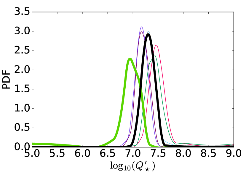
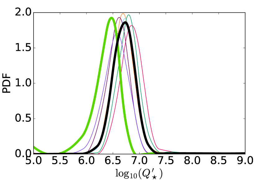
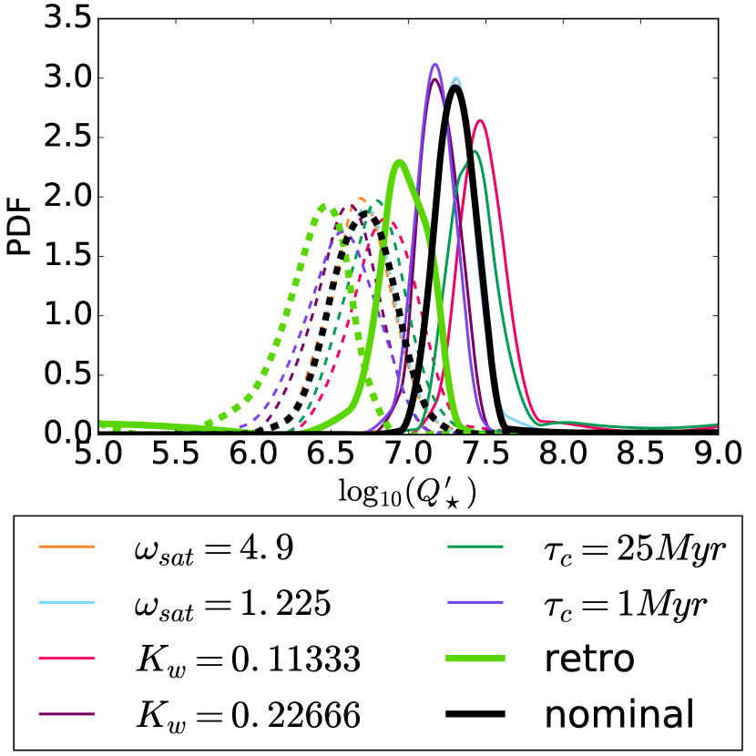
In order to generate plots of the probability density functions (PDF) derived by the procedure described above, we fit a smoothing bicubic spline to the cumulative distribution with a tiny amount of smoothing in order to suppress numerical oscillations when taking the derivative. Fig. 10 shows the PDF derived for $\log_{10}(Q^{\prime}_{\star})$ for HATS-18 and WASP-19 with the various models of table 5.2. The constraints obtained for $Q^{\prime}_{\star}$ are given in the last column of that table. The confidence interval was derived by evaluating the inverse cumulative distribution function for $\log_{10}(Q^{\prime}_{\star})$ at 15.87% and at 84.13%.

Since most of the orbital decay happens at late times when the star is evolving only very slowly on the main sequence, it is a very good approximation to assume a non–evolving star with the present properties in the last Gyr or so of the evolution. As a result, as long as the star is started with the spin predicted by angular momentum loss in the absence of a planet, the results are only very slightly sensitive to the exact stellar evolution models used. In particular this means that the exact stellar age determined by matching the evolution models to the present star, has only a very small effect on the results.

Clearly, parametrizing tidal dissipation by a single number ($Q^{\prime}_{\star}$ in our case) is a gross oversimplification of the physics involved. In reality $Q^{\prime}_{\star}$ should depend on the stellar mass, the tidal frequency, and the stellar spin. This can affect the results in two ways: first, it could be one way to explain the different results obtained for the two systems, and second, even for a single system, the spin of the star and the tidal frequency evolve, thus different tidal dissipation will operate at different times during the system’s past. However, for the two planetary systems considered all these parameters are currently almost identical. Further, due to the strong dependence of the rate of orbital decay on the planet–star separation, and the fact that angular momentum loss is faster for faster spinning stars, only the most recent part of the evolution of the systems matters (as demonstrated in Fig. 9).

So even though the past spin histories of the two stars may have been somewhat different (due to the different planetary masses), this has a relatively small impact on the results. In addition, since the evolution is dominated by the latest stages, strictly speaking, the constraints derived here give the tidal quality factor for parameters close to the currently observed ones (a stellar mass of approximately a $1M_{\odot}$, for orbital periods of approximately 0.8 days and for stellar spin periods of about 10 days). Finally, this also means that the formation mechanism for the planets is irrelevant for the derived constraints. While it is true that starting the orbital evolution later, if planet migration is delayed, can decrease the amount of angular momentum added to the star, this is a totally negligible effect (see Fig. 9).

Disentangling the dependence of the tidal dissipation on some of these quantities may be possible by performing similar analysis on a larger number of exoplanet systems, ideally all currently known extremely short period ones. In addition, orbital circularization and spin synchronization in open cluster binaries is able to probe much longer orbital periods than is feasible with extrasolar planets.

6. Discussion

HATS-18 is an extreme short–period planet which is among the best targets for testing theories of planet–star interactions. In fact, the host star, like a number of other extremely short period giant–planet hosts (e.g. WASP-19 above, WASP-103 (Gillon et al., 2014), OGLE-TR-113 (Bouchy et al., 2004)) appears to be spinning too fast for its age. HATS-18 is the best system to–date for constraining the stellar tidal dissipation by assuming that the extra stellar angular momentum was delivered by tidal decay of the orbit. In fact, we applied this method to the two exoplanet systems whose host stars should have been spun up the most, and which have very similar properties, to derive tight constraints on the stellar tidal quality factor at least in the regime applicable to those systems. In fact, if both of these planets are assumed to have formed in orbits well aligned with their parent star’s spin, there is only a very narrow range around $\log_{10}(Q^{\prime}_{\star})=7$ for which the present spin period of both stars is at least marginally consistent with the expected degree of spin–up. This tight constraint will also apply if planets form with a wide range of initial obliquities, but are quickly re-aligned by some process which operates on timescales short compared to the orbital decay. On the other hand, if planets are assumed to form with a wide range of obliquities, and if at least for the extremely short periods of HATS-18 and WASP-19, the timescale for orbital decay is shorter than any processes which tend to align the orbit with the stellar equator, it is plausible that WASP-19 started out in a well aligned orbit, while HATS-18 was significantly misaligned in which case, $6.5<\log_{10}(Q^{\prime}_{\star})<7$. Clearly, a more systematic effort to analyze all suitable exoplanet systems and properly account for the stellar angular momentum loss uncertainties is bound to yield very meaningful constraints on the stellar tidal dissipation, as well how it changes with various system properties.

These constraints do not match the recently suggested detection of orbital decay in WASP-12 (Maciejewski et al., 2016), which would correspond to a tidal quality factor of $Q^{\prime}_{\star}=2.5\times 10^{5}$. However, the authors of that study point out that at present the observed period change is still marginally consistent with apsidal precession. Further, as we pointed out above, the tidal quality factor is not expected to be the same across different systems, and WASP-12 differs from both HATS-18 and WASP-19 in several important respects: it has a hotter star, with only a minimal surface convective zone, and it appears to be spinning significantly slower. Both of these properties are expected to impact the tidal dissipation. The same measurement is also within reach for HATS-18b. For example, after 28 years, the time of arrival of HATS-18b transits will have shifted by 60 s if $Q^{\prime}_{\star}=10^{7}$ due to tidal orbital decay, thus making it feasible to measure.

As we argued in § 4, extremely short period planets like HATS-18 provide a fantastic laboratory to test a range of interactions between the planet and the star, and hence, expanding this sample is extremely valuable for the study of extrasolar planets.

Acknowledgements

Development of the HATSouth project was funded by NSF MRI grant NSF/AST-0723074, operations have been supported by NASA grants NNX09AB29G and NNX12AH91H, and follow-up observations received partial support from grant NSF/AST-1108686. K.P. acknowledges support from NASA grants NNX13AQ62G and NNG14FC03C. G.B. acknowledges support from the David and Lucile Packard Foundation, from NASA grants NNX13AJ15G, NNX14AF87G and NNX13AQ62G. J.H. acknowledges support from NASA grants NNX13AJ15G and NNX14AF87G. R.B. and N.E. are supported by CONICYT-PCHA/Doctorado Nacional. A.J. acknowledges support from FONDECYT project 1130857, BASAL CATA PFB-06, and from the Ministry of Economy, Development, and Tourism’s Millenium Science Initiative through grant IC120009, awarded to the Millenium Institute of Astrophysics, MAS. R.B. and N.E. acknowledge additional support from the Ministry of Economy, Development, and Tourism’s Millenium Science Initiative through grant IC120009, awarded to the Millenium Institute of Astrophysics, MAS. V.S. acknowledges support from BASAL CATA PFB-06. This paper uses observations obtained with facilities of the Las Cumbres Observatory Global Telescope. Work at the Australian National University is supported by ARC Laureate Fellowship Grant FL0992131. We acknowledge the use of the AAVSO Photometric All-Sky Survey (APASS), funded by the Robert Martin Ayers Sciences Fund, and the SIMBAD database, operated at CDS, Strasbourg, France. Operations at the MPG 2.2 m Telescope are jointly performed by the Max Planck Gesellschaft and the European Southern Observatory. G. B. wishes to thank the warm hospitality of Adéle and Joachim Cranz at the farm Isabis, supporting the operations and service missions of HATSouth.

References

- Agüeros et al. (2011) Agüeros, M. A., Covey, K. R., Lemonias, J. J., et al. 2011, ApJ, 740, 110
- Albrecht et al. (2012) Albrecht, S., Winn, J. N., Johnson, J. A., et al. 2012, ApJ, 757, 18
- Amard et al. (2016) Amard, L., Palacios, A., Charbonnel, C., Gallet, F., & Bouvier, J. 2016, A&A, 587, A105
- Bakos et al. (2010) Bakos, G. Á., Torres, G., Pál, A., et al. 2010, ApJ, 710, 1724
- Bakos et al. (2013) Bakos, G. Á., Csubry, Z., Penev, K., et al. 2013, PASP, 125, 154
- Barnes et al. (2016) Barnes, S. A., Weingrill, J., Fritzewski, D., & Strassmeier, K. G. 2016, ArXiv e-prints, 1603.09179
- Bayliss et al. (2013) Bayliss, D., Zhou, G., Penev, K., et al. 2013, AJ, 146, 113
- Bouchy et al. (2004) Bouchy, F., Pont, F., Santos, N. C., et al. 2004, A&A, 421, L13
- Brahm et. al. (2016) Brahm et. al., . 2016
- Cardelli et al. (1989) Cardelli, J. A., Clayton, G. C., & Mathis, J. S. 1989, ApJ, 345, 245
- Claret (2004) Claret, A. 2004, A&A, 428, 1001
- Dawson & Murray-Clay (2013) Dawson, R. I., & Murray-Clay, R. A. 2013, ApJ, 767, L24
- Delorme et al. (2011) Delorme, P., Collier Cameron, A., Hebb, L., et al. 2011, MNRAS, 413, 2218
- Demarque et al. (2008) Demarque, P., Guenther, D. B., Li, L. H., Mazumdar, A., & Straka, C. W. 2008, Ap&SS, 316, 31
- Dopita et al. (2007) Dopita, M., Hart, J., McGregor, P., et al. 2007, Ap&SS, 310, 255
- Fossati et al. (2010) Fossati, L., Haswell, C. A., Froning, C. S., et al. 2010, ApJ, 714, L222
- Fressin et al. (2013) Fressin, F., Torres, G., Charbonneau, D., et al. 2013, ApJ, 766, 81
- Gallet & Bouvier (2015) Gallet, F., & Bouvier, J. 2015, A&A, 577, A98
- Gillon et al. (2014) Gillon, M., Anderson, D. R., Collier-Cameron, A., et al. 2014, A&A, 562, L3
- Ginzburg & Sari (2015) Ginzburg, S., & Sari, R. 2015, ApJ, 803, 111
- Hansen & Barman (2007) Hansen, B. M. S., & Barman, T. 2007, ApJ, 671, 861
- Hartman et al. (2010) Hartman, J. D., Bakos, G. Á., Kovács, G., & Noyes, R. W. 2010, MNRAS, 408, 475
- Hartman et al. (2009) Hartman, J. D., Gaudi, B. S., Pinsonneault, M. H., et al. 2009, ApJ, 691, 342
- Hartman et al. (2012) Hartman, J. D., Bakos, G. Á., Béky, B., et al. 2012, AJ, 144, 139
- Haswell et al. (2012) Haswell, C. A., Fossati, L., Ayres, T., et al. 2012, ApJ, 760, 79
- Hebb et al. (2010) Hebb, L., Collier-Cameron, A., Triaud, A. H. M. J., et al. 2010, ApJ, 708, 224
- Ida & Lin (2008) Ida, S., & Lin, D. N. C. 2008, ApJ, 673, 487
- Irwin et al. (2009) Irwin, J., Aigrain, S., Bouvier, J., et al. 2009, MNRAS, 392, 1456
- Irwin et al. (2007) Irwin, J., Hodgkin, S., Aigrain, S., et al. 2007, MNRAS, 377, 741
- Jordán et al. (2014) Jordán, A., Brahm, R., Bakos, G. Á., et al. 2014, AJ, 148, 29
- Kaufer & Pasquini (1998) Kaufer, A., & Pasquini, L. 1998, in Society of Photo-Optical Instrumentation Engineers (SPIE) Conference Series, Vol. 3355, Optical Astronomical Instrumentation, ed. S. D’Odorico, 844–854
- Kovács et al. (2005) Kovács, G., Bakos, G., & Noyes, R. W. 2005, MNRAS, 356, 557
- Kovács et al. (2002) Kovács, G., Zucker, S., & Mazeh, T. 2002, A&A, 391, 369
- Kovács et al. (2014) Kovács, G., Hartman, J. D., Bakos, G. Á., et al. 2014, MNRAS, 442, 2081
- Lai (2012) Lai, D. 2012, MNRAS, 423, 486
- Maciejewski et al. (2016) Maciejewski, G., Dimitrov, D., Fernández, M., et al. 2016, A&A, 588, L6
- Mandel & Agol (2002) Mandel, K., & Agol, E. 2002, ApJ, 580, L171
- Penev et al. (2012) Penev, K., Jackson, B., Spada, F., & Thom, N. 2012, ApJ, 751, 96
- Penev et al. (2014) Penev, K., Zhang, M., & Jackson, B. 2014, PASP, 126, 553
- Penev et al. (2013) Penev, K., Bakos, G. Á., Bayliss, D., et al. 2013, AJ, 145, 5
- ter Braak (2006) ter Braak, C. J. F. 2006, Statistics and Computing, 16, 239
- Tregloan-Reed et al. (2013) Tregloan-Reed, J., Southworth, J., & Tappert, C. 2013, MNRAS, 428, 3671
- Yi et al. (2001) Yi, S., Demarque, P., Kim, Y.-C., et al. 2001, ApJS, 136, 417