On the Geometry of the Hamilton–Jacobi Equation
and
Generating Functions

Abstract

In this paper we develop a geometric version of the Hamilton–Jacobi equation in the Poisson setting. Specifically, we “geometrize” what is usually called a complete solution of the Hamilton–Jacobi equation. We use some well-known results about symplectic groupoids, in particular cotangent groupoids, as a keystone for the construction of our framework. Our methodology follows the ambitious program proposed by A. Weinstein, [62], in order to develop geometric formulations of the dynamical behavior of Lagrangian and Hamiltonian systems on Lie algebroids and Lie groupoids. This procedure allows us to take symmetries into account, and, as a by-product, we recover results from [14, 29, 31], but even in these situations our approach is new. A theory of generating functions for the Poisson structures considered here is also developed following the same pattern, solving a longstanding problem of the area: how to obtain a generating function for the identity tranformation and the nearby Poisson automorphisms of Poisson manifolds. A direct application of our results give the construction of a family of Poisson integrators, that is, integrators that conserve the underlying Poisson geometry. These integrators are implemented in the paper in benchmark problems. Some conclusions, current and future directions of research are shown at the end of the paper.

Keywords: Hamilton-Jacobi theory, symplectic groupoids, Lagrangian submanifolds, symmetries, Poisson manifolds, Poisson integrators, generating functions.

1 Introduction

1.1 Motivation

To find canonical changes of coordinates that reduce the Hamiltonian function to a form such that the equations can be easily integrated is a very useful procedure for the integration of the classical Hamilton’s equations. As a consequence, this shows that the initial equations are integrable. But, of course, the main problem is to find these particular canonical transformations. This problem is equivalent to the determination of a large enough number of solutions of the Hamilton–Jacobi equation. This is the objective of the representation of canonical transformations in terms of generating functions and leads to complete solutions of the Hamilton–Jacobi equations. The usefulness of this method is highlighted in the following quote by V.I. Arnold, (see [2], p. 233):

“The technique of generating functions for canonical transformations, developed by Hamilton and Jacobi, is the most powerful method available for integrating the differential equations of dynamics.”

-V.I. Arnold

The procedure described above is well-known in the classical case, which geometrically corresponds to the cotangent bundle of the configuration manifold under consideration (we remark that a recent geometric Hamilton-Jacobi theory, which includes Lagrangian and Hamiltonian systems, was developed in [9]). Some research has been also done in the Lie–Poisson case ([31]) as well. The goal of the following exposition is to introduce these two cases in order to motivate our future constructions, which deepen and generalize these results in a highly non-trivial way finding new and powerful applications.

1.1.1 The Classical Case

Let $Q$ be the $n$-dimensional configuration manifold of a mechanical system and let $(T^{*}Q,\ \omega_{Q},\ H)$ be a Hamiltonian system. In this system $\omega_{Q}$ is the canonical symplectic structure of the cotangent bundle, $T^{*}Q$. Along this paper $\pi_{Q}:T^{*}Q\rightarrow Q$ will be the natural projection of the cotangent bundle onto $Q$, and $H:T^{*}Q\rightarrow\mathbb{R}$ will denote the Hamiltonian function. Associated with such a Hamiltonian there is a Hamiltonian vector field, $X_{H}$, defined by $i_{X_{H}}\omega_{Q}=dH$. In natural cotangent coordinates $(q^{i},p_{i})$ the symplectic structure reads $\omega_{Q}=dq^{i}\wedge dp_{i}$ and the Hamiltonian vector field becomes

$$X_{H}(q^{i},p_{i})=\displaystyle\frac{\partial H}{\partial p_{i}}(q^{i},p_{i})\frac{\partial}{\partial q^{i}}-\frac{\partial H}{\partial q^{i}}(q^{i},p_{i})\frac{\partial}{\partial p_{i}},$$

so the equations of motion read

$$\begin{array}[]{rl}\displaystyle\frac{dq^{i}}{dt}(t)=&\displaystyle\frac{\partial H}{\partial p_{i}}(q^{i}(t),p_{i}(t)),\\ \vskip 12.0pt plus 4.0pt minus 4.0pt\cr\displaystyle\frac{dp_{i}}{dt}(t)=&-\displaystyle\frac{\partial H}{\partial q^{i}}(q^{i}(t),p_{i}(t)),\end{array}$$ (1)

for $i=1,\ldots,\ n$.

For the sake of simplicity, and in order to clarify the main ideas of the paper, we start with a local coordinate description. Those ideas hold locally for any symplectic manifold in Darboux coordinates. The reader interested in the details and proofs of the results presented here is referred to [1, 2, 32]. Assume that we have found a function $S$ that depends on the time, $t$, the $(q^{i})$-coordinates and $n$ parameters, say $(x^{i})$, $1\leq i\leq n$, so $S=S(t,q^{i},x^{i})$, satisfying the following two conditions:

1. Hamilton–Jacobi equation:

   $$\frac{\partial S}{\partial t}(t,q^{i},x^{i})+H(q^{i},\frac{\partial S}{\partial q^{i}}(t,q^{i},x^{i}))=K(t,x^{i}),$$ (2)

   where $K$ is a function that only depends on $t$ and $x^{i}$;

2. Non-degeneracy condition: $\det(\displaystyle\frac{\partial^{2}S}{\partial q^{i}\partial x^{j}})\neq 0$,

then, by the implicit function theorem we can make the following change of coordinates $(t,q^{i},p_{i})\rightarrow(t,x^{i},y_{i})$ defined implicitly by

$$\begin{array}[]{cc}\displaystyle\frac{\partial S}{\partial q^{i}}(t,q^{i},x^{i})=p_{i},&-\displaystyle\frac{\partial S}{\partial x^{i}}(t,q^{i},x^{i})=y_{i}.\end{array}$$ (3)

After some brief computations, one can see that in the new coordinates $(t,x^{i},y_{i})$ the equations of motion are again in Hamiltonian form, but now the Hamiltonian is the function $K(t,x^{i})$, i.e. the equations (1) read now

$$\begin{array}[]{rl}\displaystyle\frac{dx^{i}}{dt}(t)=&\displaystyle\frac{\partial K}{\partial y_{i}}(t,x^{i}(t))=0,\\ \vskip 12.0pt plus 4.0pt minus 4.0pt\cr\displaystyle\frac{dy_{i}}{dt}(t)=&-\displaystyle\frac{\partial K}{\partial x^{i}}(t,x^{i}(t)),\end{array}$$ (4)

for $i=1,\ldots,\ n$.

Since $K$ only depends on the time and the $(x^{i})$-coordinates, these equations are trivially integrable. Given an initial condition $(x^{i}_{0},y_{i}^{0})$ at time $t_{0}$, the curve

$$t\rightarrow\Big{(}x^{i}_{0},y_{i}^{0}-\int_{t_{0}}^{t}\displaystyle\frac{\partial K}{\partial x^{i}}(t,x^{i}_{0})dt\Big{)}$$

is the solution of equations (4) with initial condition $(x^{i}_{0},y_{i}^{0})$.

Remark 1.

The equation

$$\frac{\partial S}{\partial t}(t,q^{i},x^{i})+H(q^{i},\frac{\partial S}{\partial q^{i}}(t,q^{i},x^{i}))=0$$ (5)

appears frequently in the literature. If one is able to find the function $S$ satisfying equation (5) and the above non-degeneracy condition, that means that $K=0$ and so the equations of motion become $\frac{dx^{i}}{dt}(t)=0$ and $\frac{dy_{i}}{dt}(t)=0$. This means that in the new coordinates the system is in “equilibrium”; it does not evolve at all! The inverse of that change of variables gives the flow, up to an initial transformation given by $S(0,q^{i},x^{i})$, later on we will clarify this claim. In general, any $S$ satisfying the non-degeneracy condition will induce a canonical transformation implicitly by the rule described above, which implies that Hamilton’s equations in the $(q^{i},p_{i})$ coordinates will remain as Hamilton’s equations in the $(x^{i},y_{i})$ coordinates for a new Hamiltonian, say $K$, which is related to the Hamilton–Jacobi equation by the expression

$$\frac{\partial S}{\partial t}+H(t,q^{i},\frac{\partial S}{\partial q^{i}})=K(t,x^{i},y_{i}).$$ (6)

Observe that equations (2) and (5) are particular instances of the last equation. We will elaborate on these and related issues in Section 3.

We proceed now to give a geometric framework for the previous procedure. A nice exposition of Lagrangian submanifolds, generating functions and related topics can be found in [7]. The function $S$, satisfying (2), is interpreted here as a function on the product manifold $\mathbb{R}\times Q\times Q$ and so $\textrm{Im}(dS)$ is a Lagrangian submanifold in $T^{*}(\mathbb{R}\times Q\times Q)$. Notice that we are thinking about the $(q^{i})$ as coordinates on the first $Q$, and $(x^{i})$ as coordinates on the second factor $Q$. This interpretation is directly related to the fact that we are describing here type I generating functions in the language of [32]. Other types of generating functions will be introduced along the next sections. On the other hand, consider the projections $\pi_{I}:T^{*}(\mathbb{R}\times Q\times Q)\rightarrow\mathbb{R}\times T^{*}Q$, $I=1,2$, defined by $\pi_{2}(t,e,x^{i},y_{i},q^{i},p_{i})=(t,q^{i},p_{i})$ and $\pi_{1}(t,e,x^{i},y_{i},q^{i},p_{i})=(t,x^{i},-y_{i})$. With these geometric tools the non-degeneracy condition is equivalent to saying that ${\pi_{I}}_{|\textrm{Im}(dS)}$ are local diffeomorphisms for $I=1,2$. We assume here for simplicity that they are global diffeomorphisms, so we can consider the mapping ${\pi_{1}}_{|\textrm{Im}(dS)}\circ({\pi_{2}}_{|\textrm{Im}(dS)})^{-1}:\mathbb{R}\times T^{*}Q\rightarrow\mathbb{R}\times T^{*}Q$. The local argument follows with the obvious restrictions to open sets. This mapping can be easily checked to be the geometric description of the change of variables introduced in (3). The Hamilton–Jacobi equation (2) can be understood as the fact that $dS^{*}(\pi_{2}^{*}H+e)$ must be equal to $pr_{1}^{*}K$ for some $K\in C^{\infty}(\mathbb{R}\times Q)$, where $pr_{I}:\mathbb{R}\times Q\times Q\rightarrow\mathbb{R}\times Q,\ I=1,\ 2$ are $pr_{1}(t,q^{i},x^{i})=(t,x^{i}),$ $pr_{2}(t,q^{i},x^{i})=(t,q^{i})$. The diagram below illustrates the situation.

Figure 1: Geometric interpretation.

The transformation ${\pi_{1}}_{|\textrm{Im}(dS)}\circ({\pi_{2}}_{|\textrm{Im}(dS)})^{-1}$ satisfies

$$\Big{(}{\pi_{1}}_{|\textrm{Im}(dS)}\circ({\pi_{2}}_{|\textrm{Im}(dS)})^{-1}\Big{)}_{*}(\frac{\partial}{\partial t}+X_{H})=\frac{\partial}{\partial t}+X_{K},$$

which is the geometric description of the transformation of equations (1) into (4).

Remark 2.

We want to call the attention of the reader familiar with Lie groupoids or discrete mechanics about the geometric structure needed to handle this theory. In the above diagram, if one removes the $\mathbb{R}$ factor, what we have is just a pair groupoid $Q\times Q$ and the corresponding cotangent groupoid $T^{*}(Q\times Q)$, with base the dual of its Lie algebroid $T^{*}Q$. We will show that the multiplication by the $\mathbb{R}$ factor conserves the groupoid and cotangent groupoid structures and for $\mathbb{R}\times Q\times Q$ the source and the target are exactly $pr_{1}$ and $pr_{2}$; furthermore, for the cotangent bundle $T^{*}(\mathbb{R}\times Q\times Q)$ the source and the target are just $\pi_{1}$ and $\pi_{2}$, introduced above.

Remark 3.

The inverse of the transformation induced above, which happens to be ${\pi_{2}}_{|\textrm{Im}(dS)}\circ({\pi_{1}}_{|\textrm{Im}(dS)})^{-1}$, up to an initial condition on $S$ at time $t=0$ gives the flow of the Hamiltonian vector field $X_{H}$.

Remark 4.

We used a time-independent Hamiltonian, but actually the theory is exactly the same for time-dependent systems.

1.1.2 The Lie–Poisson Case

In this section we write in a geometric way the results about Hamilton–Jacobi theory for Lie–Poisson systems, $(\mathfrak{g}^{*},\ \Lambda,\ H)$, where

1. $\mathfrak{g}^{*}$ is the dual of the Lie algebra $\mathfrak{g}$ of a Lie group $G$.

2. $\Lambda$ is the canonical (-) Poisson structure on $\mathfrak{g}^{*}$, given by

   $$\{f,g\}(\mu)=-\mu([df(\mu),dg(\mu)])=\Lambda(df,dg)(\mu);$$

   where $f,\ g:\ \mathfrak{g}^{*}\rightarrow\mathbb{R}$ and $\mu\in\mathfrak{g}^{*}$.

3. $H:\mathfrak{g}^{*}\rightarrow\mathbb{R}$ is a Hamiltonian function.

These objects produce a dynamical system through the equation

$$\dot{\mu}=X_{H}(\mu)=\Lambda^{\sharp}(dH)(\mu),$$

where $df(\Lambda^{\sharp}(dH))=\Lambda(df,dH)$, and $X_{H}$ is called the Hamiltonian vector field. Detailed information about Lie–Poisson systems can be found, for instance, in [45]. Similar results to the ones that we are going to introduce now appeared for the first time in [31], related information can also be found in [42]. Nonetheless, the approaches followed in those works are very different and even in these situations we will give new results. In order to continue we need to define some mappings. The left and right momentum are the mappings $J_{L}:T^{*}G\rightarrow\mathfrak{g}^{*}$ and $J_{R}:T^{*}G\rightarrow\mathfrak{g}^{*}$ defined by $\langle J_{L}(\alpha_{g}),\xi\rangle=\langle\alpha_{g},T_{\mathfrak{e}}R_{g}(\xi)\rangle$ and $\langle J_{R}(\alpha_{g}),\xi\rangle=\langle\alpha_{g},T_{\mathfrak{e}}L_{g}(\xi)\rangle$. Let $S:\mathbb{R}\times G\rightarrow\mathbb{R}$ be a function such that the following conditions hold:

1. Hamilton–Jacobi equation: $\displaystyle\frac{\partial S}{\partial t}(t,g)+H(J_{R}\circ dS_{t})=k(t)$, where $S_{t}$ is defined by $S_{t}(g)=S(t,g)$.

2. Non-degeneracy condition: let $\xi_{a}$ be a basis of $\mathfrak{g}$. Then we assume that $\overleftarrow{\xi}_{a}(\overrightarrow{\xi}_{b}(S_{t}))$ is a regular matrix. Here $\overleftarrow{\xi}_{a}$ and $\overrightarrow{\xi}_{b}$ are the associated left-invariant and right-invariant vector fields respectively.

With the function $S$ at hand we can define a transformation analogous to (3). To make the exposition easier, we introduce the following diagram analogous to diagram in Figure 1:

Figure 2: Lie-Poisson Setting.

where $(\operatorname{id}_{\mathbb{R}}\times J_{L})(t,e,\alpha_{g})=(t,J_{L}(\alpha_{g}))$ and, in the same manner, we define $\operatorname{id}_{\mathbb{R}}$ $\times J_{R}$. The Hamilton–Jacobi equation is equivalent to saying that $dS^{*}((\operatorname{id}_{\mathbb{R}}\times J_{R})^{*}(H+e))$ is equal to a time-dependent function $k(t)$. It can also be checked that the non-degeneracy condition implies that $\operatorname{id}_{\mathbb{R}}\times J_{L}$ restricted to $\textrm{Im}(dS)$ is a local diffeomorphism (it turns out that this is equivalent to that $\operatorname{id}_{\mathbb{R}}\times J_{R}$ restricted to $\textrm{Im}(dS)$ to be a local diffeomorphism). Now we can define the Poisson mapping $(\operatorname{id}_{\mathbb{R}}\times J_{L})\circ(\operatorname{id}_{\mathbb{R}}\times{J_{R}}_{|\textrm{Im}(dS)})^{-1}:\mathbb{R}\times\mathfrak{g}^{*}\rightarrow\mathbb{R}\times\mathfrak{g}^{*}$, henceforth denoted by $\hat{S}$. In this way we complete the diagram in Figure 2 as follows:

Figure 3: Geometric interpretation.

The main fact is, again, that $\hat{S}:\mathbb{R}\times\mathfrak{g}^{*}\rightarrow\mathbb{R}\times\mathfrak{g}^{*}$ verifies

$$\hat{S}_{*}(\frac{\partial}{\partial t}+X_{H})=\frac{\partial}{\partial t},$$

which means that the Hamiltonian evolution is transformed into the trivial dynamics. With this method, we achieve a Poisson transformation which completely integrates the dynamics.

Remark 5.

If we think about the underlying geometric structure, forgetting about the $\mathbb{R}$ factor, we have a Lie group, $G$, and its cotangent groupoid $T^{*}G$. The source and target of this cotangent groupoid are known to be the mappings $J_{L}$ and $J_{R}$. We will see that $T^{*}(\mathbb{R}\times G)$ is again a (symplectic) groupoid and that $\operatorname{id}_{\mathbb{R}}\times J_{L}$ and $\operatorname{id}_{\mathbb{R}}\times J_{R}$ are its source and target.

Remark 6.

As in the standard case, the Hamiltonian can be time-dependent and the same results hold.

With these two examples at hand it seems clear that the geometry of the theory can be described using cotangent Lie groupoids. The idea of using Lie groupoids to describe the Hamilton–Jacobi equation appeared for the first time in [29], as far as we know, and there it is pointed out that A. Weinstein was the first to notice that there may be a connection between generating functions and symplectic groupoids. As opposed to that general approach, we focus on giving a complete picture in the case of cotangent Lie groupoids. Cotangent Lie groupoids seem to be general enough to include all the interesting cases of mechanical systems, but at the same time they have interesting features that make them very useful in practical problems, which is our final goal. For instance, Darboux coordinates in the cotangent groupoid are always available, but finding them is not such an easy task in the case of a general symplectic groupoid. Furthermore, cotangent groupoids provide the natural framework to relate continuous and discrete Hamiltonian and Lagrangian dynamics, as was pointed by A. Weinstein in [62], following [53]. This viewpoint was exploited by some of the authors in [39, 40, 41]. A particular case of cotangent groupoid, the cotangent groupoid of an action Lie algebroid, was already suggested as the correct setting for a Hamilton–Jacobi theory in [59], although no more progress has been made in this direction so far. Moreover, in [59] the authors develop a finite-dimensional Poisson truncation, i.e. a finite-dimensional Poisson model of the Poisson–Vlasov equation, an infinite-dimensional Poisson system. It turns out that the truncation happens to be the dual algebroid of an action groupoid, which is a particular case of the theory that we present here. The importance of the “oid theory” was already clear to the authors

“Our first derivation used the theory of Lie groupoids and Lie algebroids, and the Poisson structures on the duals of Lie algebroids. We were then able to eliminate the “oid” theory in favor of more well-known ideas on Poisson reduction. […] The groupoid aspect of the theory also provides natural Poisson maps, useful in the application of Ruth type integration techniques, which do not seem easily derivable from the general theory of Poisson reduction”.

-C. Scovel and A. Weinstein [59], p. $683$.

Here we use that connection, symplectic groupoid–Poisson manifolds, to develop a general theory for Hamiltonian systems on the dual of an integrable Lie algebroid, a framework large enough to study all interesting Poisson Hamiltonian systems in classical mechanics. Using some well-known facts about symplectic groupoids, like the fact that the cotangent bundle of a Lie groupoid is a symplectic groupoid with base the dual bundle of the associated Lie algebroid, then, a construction similar to the one outlined in the two examples above leads to the desired Hamiton–Jacobi theory. This theory allows us to seek for transformations which integrate Hamilton’s equations in the same way we described above.

We remak that, very recently, in [33] the authors develop a geometric Hamilton-Jacobi theory for dynamical systems on the total space of a fibration. In the particular case when the dynamical system is Hamiltonian with respect to an (arbitrary) Poisson structure and the fibration is isotropic, they discuss some applications of the theory to the integration by quadratures of the system. It is clear that our approach in this paper is different. In fact, we are not concerned with the integration by quadratures of the system and, in addition, we focus on Hamiltonian systems with respect to linear Poisson structures on vector bundles. This fact, as we mentioned before, allows us to use the theory of Lie algebroids and groupoids and to discuss the interesting examples for Classical Mechanics, namely, Hamiltonian systems on cotangent bundles, on the dual space of Lie algebras and the dual bundles of action and Atiyah Lie algebroids. We also want to stress that besides the exact integration of the Hamilton’s equations our motivation comes from the applications to numerical methods, which aims to develop, among other things, the Ruth type integrators pointed in the last quote, taken from [59]. Our examples go into this direction, although the analytical and dynamical applications should be exploited as well (see the last section). It is well-known that the theory of generating functions gives a family of symplectic numerical methods, [22, 34, 50]. There are numerous examples illustrating the superior preservation of phase-space structures and qualitative dynamics by symplectic integrators. These methods were extended to Lie groups in [31], but our approach is general enough to provide a general setting to develop new numerical methods on the dual bundle of Lie algebroids. We also stress the importance of this task, extending the symplectic integrators to the Poisson world, by a Peter Lax’s quote that can be found in [22].

“In the late 1980s Feng Kang proposed and developed so-called symplectic algorithms for solving equations in Hamiltonian form. Combining theoretical analysis and computer experimentation, he showed that such methods, over long times, are much superior to standard methods. At the time of his death, he was at work on extensions of this idea to other structures.”

- P. Lax

Our approach also differs from the previous ones, [6, 14, 30, 31, 35, 51], in that we focus on the Lagrangian submanifolds instead of the generating functions themselves. We understand generating functions, as it has been done for many decades, as a device to describe Lagrangian submanifolds which are “horizontal” regarding a certain projection. That projection will only be defined locally in many cases, but that is enough for our applications. Let us clarify a little bit the situation. The most basic instance of this setting is the cotangent bundle $(T^{*}Q,\ \omega_{Q})$ endowed with the canonical symplectic structure and the natural projection $\pi_{Q}:T^{*}Q\rightarrow Q$. Then, we say that a Lagrangian submanifold, say $\mathcal{L}$, is horizontal for $\pi_{Q}$ if $(\pi_{Q})_{|\mathcal{L}}:\mathcal{L}\rightarrow Q$ is a diffeomorphism, equivalently, if there exists a closed $1$-form $\gamma$ such that $\textrm{Im}(\gamma)=\mathcal{L}$. This fact is a straightforward application of the implicit function theorem. By the Poincaré Lemma, at least locally, there exists $S$ defined on an open set of $Q$ such that $dS=\gamma$. In this sense, all the information of the Lagrangian submanifold $\mathcal{L}$ can be encoded in a function, much easier to handle. Conditions on $\mathcal{L}$ become PDEs in the unknown function $S$. This simple fact allowed us to come with analogues of the non-free canonical transformations, following the notation in [2]. They permit, in a very natural way, to generate the identity transformation as generating functions. This was an open problem, unsolved as far as we know:

“Is there a generating function for Lie–Poisson maps which generates the identity map via the coadjoint action of the identity group element?”

-R.I. McLachlan and C. Scovel. [51], p. $157$.

This result is quite useful, as the classical type I generating functions are not enough even in the classical case for may practical applications. In that regard, we would like to stress that the importance of our construction relies not on parametrizing the Lagrangian submanifolds of identities, but on giving a parametrization of all the Lagrangian submanifolds that are close to the identity. Those Lagrangian submanifolds induce the Poisson transformations which are near the identity ı.e. the Hamiltonian flow for small enough time (see Section 3.6). In addition, the results in Section $3$ and $4$ are the keystones to develop the geometric numerical methods in Section $5$. Furthermore, we give here results that show how Hamilton’s equations change under a canonical transformation induced by a generating function, generalizing the equation (6) which is needed to develop Ruth type integrators. We also show local existence of solution and generalize the classical result which claims that the action functional ($\int L\,dt$) is a solution of the Hamilton–Jacobi equation. Our approach is new even when applied to the known situations.

1.2 Summary

After the previous section, where we illustrated the motivation that led us to our results, we proceed in the following way.

Section $2$ is devoted to the definition of symplectic groupoids. We include two appendices about Lie groupoids and Lie algebroids with all the definitions and properties, so the reader unfamiliar with them should find there the information needed to understand this paper. We summarize some of the most important properties of symplectic groupoids because we are going to use them in Section 3 to develop our Hamilton–Jacobi theory. We provide several examples of symplectic groupoids and describe carefully the ones we are concerned with, cotangent groupoids.

In Section $3$ we develop the main results of this paper. The main goal is to provide a theory of generating functions and a Hamilton–Jacobi theory that allow us to look for transformations which integrate the Hamiltonian equations of motion, or at least, approximate them through Poisson automorphisms. This is done using the symplectic groupoid structure of the cotangent bundle of a groupoid, in particular, its dual pair structure. We also summarize some of the results in [31] related to these generating functions.

In Section $4$ we give a couple of results about local existence of solutions of the Hamilton–Jacobi equation introduced in the previous section. Since we are dealing with a PDE, it is our duty to show, at least, local existence of solutions. The first result generalizes the classical Jacobi’s solution of the Hamilton–Jacobi equation given by the action. The second one is the method of characteristics, well-known in the literature.

Examples are given in Section $5$. Of course, our theory recovers the classical situation via the pair groupoid and Ge–Marsden’s framework via the Lie group case. Even in those cases, our approach clarifies the geometry and our results are stronger. We present here a general procedure to apply in order to develop numerical methods. The methods are very general and apply to any Poisson manifold under consideration, but they can be drastically improved when applied to concrete situations. Moreover, all the needed tools to design new numerical methods are also presented in this paper (see the last section). The examples given in the paper are the rigid body, the heavy top and Elroy’s beanie.

2 Symplectic Groupoids

Along this section we introduce the geometric framework that allows us to “geometrize” the Hamilton–Jacobi equation in the next section. The basic definitions and properties are given and several examples are provided. The usual definitions and notation about Lie groupoids and Lie algebroids are given in the appendices A and B. The basic references for this section are [8, 16, 17]. We want to warn the reader, especially the one non experienced with groupoids, that in the end our constructions rely on the geometric structures of cotangent groupoids and not in the algebraic ones. That is, in order to follow our results it is enough to understand how to obtain the source and target of the cotangent groupoid and the results of Section 2.4. The main point is that cotangent groupoids provide a symplectic realization of the involved Poisson structures in a way that allows to control their Poisson automorphisms. To what extent the algebraic structures, multiplication and inversion, play a role here is still unknown to us.

2.1 Definition of Symplectic Groupoids

Let us now introduce the notion of a symplectic groupoid. For the definitions of groupoids, Lie groupoids or Lie algebroids and the corresponding notation see the appendices.

Definition 1.

A symplectic groupoid is a Lie groupoid $G\rightrightarrows M$ equipped with a symplectic form $\omega$ on $G$ such that the graph of the multiplication $m\ \colon\ G_{2}\to G$, that is, the set $\left\{(g,h,gh)\,|\,(g,h)\in G_{2}\right\}$, is a Lagrangian submanifold of $G\times G\times(-G)$ with the product symplectic form, where $-G$ denotes $G$ endowed with the symplectic form $-\omega$.

Remark 7.

It can be easily check that $(G,\omega)$ is a symplectic groupoid in the above sense if and only if the $2$-form $\omega$ is multiplicative. We say that the form $\omega$ is multiplicative iff

$$m^{*}\omega=\pi_{1}^{*}\omega+\pi_{2}^{*}\omega$$

where $\pi_{i}:G_{2}\rightarrow G$, $i=1,\ 2$ are the projections over the first and second factor.

2.2 Cotangent Groupoids

This section constitutes a source of examples of symplectic groupoids. Since cotangent groupoids play an important role in our theory they deserve a whole subsection. Assume that $G\rightrightarrows M$ is a Lie groupoid with source and target $\alpha$ and $\beta$ respectively and identity section, inversion map and multiplication $\epsilon$, $\iota$ and $m$, then there is an induced Lie groupoid structure $T^{*}G\rightrightarrows A^{*}G$ which we define below (see Appendix B for notation). The cotangent bundle $T^{*}G$ turns out to be a symplectic groupoid with the canonical symplectic form $\omega_{G}$ (see [16, 17]). Let us define the composition law on $T^{*}G$, which will be written as $\oplus_{T^{*}G}$, and let $\widetilde{\alpha}$, $\widetilde{\beta}$, $\widetilde{\epsilon}$ and $\widetilde{\iota}$ stand for the source, target, identity section and inversion map of the groupoid structure on $T^{*}G$ defined below. Each one of these maps will cover the corresponding structural map of $G$.

1. The source is defined in a way that the following diagram is commutative

   (7)

   Assume that $g\in G^{x}_{y}=\alpha^{-1}(x)\cap\beta^{-1}(y)$ and let $X\in A_{x}G$. So, by the definition of Lie algebroid associated to a Lie groupoid, $X$ is a tangent vector at $\epsilon(x)$ that is tangent to $G^{x}=\alpha^{-1}(x)$. Then, since $\iota\ \colon\ G^{x}\rightarrow G_{x}$ (where $G_{x}=\beta^{-1}(x)$) is a diffeomorphism between the $\alpha$-fibers and $\beta$-fibers, we conclude that $-(T_{\epsilon(x)}\iota)(X)\in T_{\epsilon(x)}G_{x}$, i.e., it is tangent to the $\beta$-fiber. Now, recalling that right multiplication is a bijection $r_{g}:G_{x}\rightarrow G_{y}$, with $g\in G^{x}_{y}$, we have that $T_{\epsilon(x)}r_{g}(-T_{\epsilon(x)}\iota(X))\in T_{g}G$ and we can finally define

   $$\widetilde{\alpha}(\varpi_{g})(X)=\varpi_{g}(-T_{\epsilon(x)}(r_{g}\circ\iota)(X)),\;\;\mbox{ for }\varpi_{g}\in T_{g}^{*}G.$$

   In particular, if we are dealing with a section $X\in\Gamma(\tau)$, the previous construction leads us to right-invariant vector fields:

   $$\widetilde{\alpha}(\varpi_{g})(X)=\varpi_{g}(\overrightarrow{X}(g)),\text{ for }X\in\Gamma(\tau),$$ (8)

   where $\tau\ \colon AG\to M$ is the Lie algebroid associated to $G$ (see equation (35) in Appendix B).

   Notice that $\widetilde{\alpha}\ \colon\ T^{*}G\to A^{*}G$ is a surjective submersion.

2. In an analogous way, the target, $\widetilde{\beta}\ \colon\ T^{*}G\to A^{*}G$, is defined so that the following diagram commutes

   (9)

   Now, given $\varpi_{g}\in T_{g}^{*}G$ and assuming that $g\in G^{x}_{y}$, since left multiplication is defined on the $\alpha$-fibers, $l_{g}\ \colon G^{y}\rightarrow G^{x}$, then $T_{\epsilon(x)}l_{g}(X)\in T_{g}G$ and we can define

   $$\widetilde{\beta}(\varpi_{g})(X)=\varpi_{g}(T_{\epsilon(x)}l_{g}(X)).$$

   In other words,

   $$\widetilde{\beta}(\varpi_{g})(X)=\varpi_{g}(\overleftarrow{X}(g)),\text{ for }X\in\Gamma(\tau)$$ (10)

   from equation (34), Appendix B.

3. The identity map, $\widetilde{\epsilon}:A^{*}G\to T^{*}G$, is defined so that

   commutes. Take $v\in T_{\epsilon(x)}G$. We can obtain an element of $A_{x}G\subset T_{\epsilon(x)}G$ by computing $v-T(\epsilon\circ\alpha)(v)$. This tangent vector is indeed tangent to an $\alpha$-fiber since $T\alpha$ of it is $0$, using an argument analogous to that in the definition of $\widetilde{\alpha}$. Then, for $\mu_{x}\in A^{*}_{x}G$, we define

   $$\widetilde{\epsilon}(\mu_{x})(v)=\mu_{x}(v-T(\epsilon\circ\alpha)(v)).$$

4. The inversion map, $\widetilde{\iota}\colon\;T^{*}G\to T^{*}G$, is defined as a mapping from each $T^{*}_{g}G$ to $T^{*}_{g^{-1}}G$. If $X\in T_{g^{-1}}G$, then $T\iota(X)\in T_{g}G$, so we can define for $\varpi_{g}\in T^{*}_{g}G$

   $$\widetilde{\iota}(\varpi_{g})(X)=-\varpi_{g}(T\iota(X)).$$

5. The groupoid operation $\oplus_{T^{*}G}$ is defined for these pairs $(\varpi_{g},\nu_{h})\in T^{*}G\times T^{*}G$ satisfying the composability condition $\widetilde{\beta}(\varpi_{g})=\widetilde{\alpha}(\nu_{h})$, which in particular implies that $(g,h)\in G_{2}$ using diagrams (7) and (9). This condition can be rewritten as

   $$\varpi_{g}\circ Tl_{g}=-\nu_{h}\circ Tr_{h}\circ T\iota\quad\text{on }A_{\beta(g)}G\subset T_{\epsilon(\beta(g))}G.$$

   We define

   $$\left(\varpi_{g}\oplus_{T^{*}G}\nu_{h}\right)(T_{(g,h)}m(X_{g},Y_{h}))=\varpi_{g}(X_{g})+\nu_{h}(Y_{h}),$$

   for $(X_{g},Y_{h})\in T_{(g,h)}G_{2}$. An explicit expression for $\oplus_{T^{*}G}$ using local bisections in the Lie groupoid $G$ can be found in [41].

Remark 8.

Note from equation (8) (resp. (10)) that the definition of $\widetilde{\alpha}$ (resp. $\widetilde{\beta}$) is just given by “translation” via right-invariant vector fields (resp. left-invariant).

Remark 9.

Another interesting property is that the application $\pi_{G}\ \colon\ T^{*}G\to G$ is a Lie groupoid morphism over the vector bundle projection $\tau_{A^{*}G}\colon A^{*}G\to M$.

Remark 10.

When the Lie groupoid $G$ is a Lie group, the Lie groupoid $T^{*}G$ is not in general a Lie group. The base $A^{*}G$ is identified with the dual of the Lie algebra $\mathfrak{g}^{*}$, and we have $\widetilde{\alpha}(\varpi_{g})(\xi)=\varpi_{g}\left(Tr_{g}\xi\right)$ and $\widetilde{\beta}(\varpi_{g})(\xi)=\varpi_{g}\left(Tl_{g}\xi\right)$, where $\varpi_{g}\in T^{*}_{g}G$ and $\xi\in{\mathfrak{g}}$.

2.3 Example: Cotangent Bundle of the Gauge Groupoid

We present now the cotangent groupoid of a gauge groupoid as an illustration of the previous constructions. The gauge groupoid is described in Section B.3.3. We assume here that the principal $G$-bundle $\pi:P\rightarrow M$ is trivial, so $P=G\times M$. Then, it is easy to see that $(P\times P)/G\equiv M\times M\times G$, with the identification $[(m^{1},g^{1},m^{2},g^{2})]\rightarrow(m^{1},m^{2},(g^{1})^{-1}g^{2})$. Thus, $T^{*}\left((P\times P)/G\right)\equiv T^{*}(M\times M\times G)$, and given $(\lambda_{m^{1}},\mu_{m^{2}},\nu_{g})\in T^{*}(M\times M\times G)$, we have

1. The source, $\tilde{\alpha}$, is the map $\tilde{\alpha}(\lambda_{m^{1}},\mu_{m^{2}},\nu_{g})=(-\lambda_{m^{1}},J_{R}(\nu_{g}))$.

2. The target, $\tilde{\beta}$, is the map $\tilde{\beta}(\lambda_{m^{1}},\mu_{m^{2}},\nu_{g})=(\mu_{m^{2}},J_{L}(\nu_{g}))$.

3. The identity map is $\tilde{\epsilon}(\lambda_{m},\nu_{g})=(-\lambda_{m},\lambda_{m},\nu_{g})$.

4. The inversion map is $\tilde{\iota}(\lambda_{m^{1}},\mu_{m^{2}},\nu_{g})=(-\mu_{m^{2}},\lambda_{m^{1}},-\nu_{g}\circ T_{g^{-1}}\iota)$, where $\iota$ is the inversion in the Lie group $G$.

5. The multiplication is $\tilde{m}\left((\lambda_{m^{1}},\mu_{m^{2}},\nu_{g}),(-\mu_{m^{2}},\mu_{m^{3}},\nu_{h})\right)=(\lambda_{m^{1}},\mu_{m^{3}},\nu_{g}\circ T_{gh}r_{h^{-1}}=\nu_{h}\circ T_{gh}l_{g^{-1}})$.

Remark 11.

Easier-to-handle expressions can be obtained by trivializing $T^{*}G\equiv G\times\mathfrak{g}^{*}$ in the product $T^{*}(M\times M\times G)\equiv T^{*}M\times T^{*}M\times T^{*}G$.

2.4 Properties

The following theorem will be crucial in the next sections (see [16, 17] for a proof, as well as the references therein):

Theorem 2.

Let $G\rightrightarrows M$ be a symplectic groupoid, with symplectic 2-form $\omega$. We have the following properties:

1. For any point $g\in G_{y}^{x}$, the subspaces $T_{g}G_{y}$ and $T_{g}G^{x}$ of the symplectic vector space $(T_{g}G,\omega_{g})$ are mutually symplectic orthogonal. That is,

   $$T_{g}G_{y}=(T_{g}G^{x})^{\perp}.$$ (11)

2. The submanifold $\epsilon(M)$ is a Lagrangian submanifold of the symplectic manifold $(G,\omega)$.

3. The inversion map $\iota\ \colon\ G\to G$ is an anti-symplectomorphism of $(G,\omega)$, that is, $\iota^{*}\omega=-\omega$.

4. There exists a unique Poisson structure $\Pi$ on $M$ for which $\beta\ \colon\ G\to M$ is a Poisson map, and $\alpha\ \colon\ G\to M$ is an anti-Poisson map (that is, $\alpha$ is a Poisson map when $M$ is equipped with the Poisson structure $-\Pi$).

Remark 12.

The theorem above states that the $\alpha$-fibers and $\beta$-fibers are symplectically orthogonal. A pair of fibrations satisfying that property are called a dual pair. This dual pair property will be the keystone of our construction.

Remark 13.

When dealing with the symplectic groupoid $T^{*}G$, where $G$ is a groupoid, the Poisson structure on $A^{*}G$ is the (linear) Poisson structure of the dual of a Lie algebroid (see Appendix A.3).

The next theorem is the core of our Hamilton–Jacobi theory. It basically says that Lagrangian bisections of a symplectic groupoid induce Poisson transformations in the base.

Theorem 3.

[see [16]] Let $G$ be a symplectic groupoid with source and target $\alpha$ and $\beta$ respectively. Let $\mathcal{L}$ be a Lagrangian submanifold of $G$ such that $\alpha_{|\mathcal{L}}$ is a (local) diffeomorphism. Then

1. $\beta_{|\mathcal{L}}:\mathcal{L}\rightarrow M$ is a (local) diffeomorphism as well.

2. The mapping $\hat{\mathcal{L}}=\alpha\circ(\beta_{|\mathcal{L}})^{-1}:M\rightarrow M$ and its inverse, $\beta\circ(\alpha_{|\mathcal{L}})^{-1}$, are (local) Poisson isomorphisms.

Remark 14.

We wrote in the above theorem the mappings in the global diffeomorphism case. Of course, when the diffeomorphism is local, these maps are restricted to the corresponding open sets.

The Lagrangian submanifolds used above are usually called Lagrangian bisections. They are bisections that happen to be Lagrangian submanifolds at the same time. See the appendices included in this paper for a definition of bisection.

3 Generating functions and Hamilton-Jacobi theory for Poisson Manifolds

3.1 The Geometric Setting

In this section we develop a theory of generating functions and a Hamilton–Jacobi theory using the geometric structures introduced along the previous sections. We encourage the reader, especially the reader not familiar with Lie groupoids and Lie algebroids, to keep in mind the two instances of the Hamilton-Jacobi theory sketched in the introduction of this paper (the classical and the Lie-Poisson cases). Our construction mimics what happens in those cases. Before going to our theory of generating function and Hamilton–Jacobi theory, we need to introduce one more construction. It basically says that the $\mathbb{R}$ factor we mentioned in Remark 2 and Remark 5 does not modify the groupoid structure. This theorem was already sketched in [29].

Proposition 4.

Let $G$ be a Lie groupoid with source, target, identity map, inversion and multiplication $\alpha,\ \beta,\ \epsilon,\ \iota$ and $m$. Then the manifold $\mathbb{R}\times G$ is a Lie groupoid with base $\mathbb{R}\times M$ and with structure mappings

$$\begin{array}[]{rccl}\alpha_{\mathbb{R}}:&\mathbb{R}\times G&\longrightarrow&\mathbb{R}\times M\\ &(t,g)&\to&\alpha_{\mathbb{R}}(t,g)=(t,\alpha(g))\\ \vskip 12.0pt plus 4.0pt minus 4.0pt\cr\beta_{\mathbb{R}}:&\mathbb{R}\times G&\longrightarrow&\mathbb{R}\times M\\ &(t,g)&\to&\beta_{\mathbb{R}}(t,g)=(t,\beta(g))\\ \vskip 12.0pt plus 4.0pt minus 4.0pt\cr\epsilon_{\mathbb{R}}:&\mathbb{R}\times M&\longrightarrow&\mathbb{R}\times G\\ &(t,x)&\to&\epsilon_{\mathbb{R}}(t,x)=(t,\epsilon(x))\\ \vskip 12.0pt plus 4.0pt minus 4.0pt\cr\iota_{\mathbb{R}}:&\mathbb{R}\times G&\longrightarrow&\mathbb{R}\times G\\ &(t,g)&\to&\iota_{\mathbb{R}}(t,g)=(t,\iota(g))\\ \vskip 12.0pt plus 4.0pt minus 4.0pt\cr m_{\mathbb{R}}:&({\mathbb{R}\times G})_{2}&\longrightarrow&\mathbb{R}\times G\\ &((t,g),(t,h))&\to&m_{\mathbb{R}}((t,g),(t,h))=(t,m(g,h)).\end{array}$$ (12)

Notice that the condition $\beta_{\mathbb{R}}(t_{1},g)=\alpha_{\mathbb{R}}(t_{2},h)$ is equivalent to $t_{1}=t_{2}$ and $\beta(g)=\alpha(h)$.

The proof is obvious and we omit it. If $AG$ is the Lie algebroid associated to $G$, then the Lie algebroid associated to $\mathbb{R}\times G$ is just $\tau_{\mathbb{R}}:\mathbb{R}\times AG\rightarrow\mathbb{R}\times M$, where $\tau_{\mathbb{R}}(t,X)=(t,\tau(X))$ and the addition is just $(t,X)+(t,Y)=(t,X+Y)$ for $t\in\mathbb{R}$ and $X,\ Y\in AG$. The anchor and the Lie bracket on sections have analogous expressions. Actually one can think of $\mathbb{R}\times G$ and $\mathbb{R}\times AG$ as “time-dependent” structures, although we regard them just as groupoids. The dual of this Lie algebroid is simply $A^{*}(\mathbb{R}\times G)=\mathbb{R}\times A^{*}G$. The cotangent bundle of $\mathbb{R}\times G$ is a (symplectic) Lie groupoid with base $\mathbb{R}\times A^{*}G$ and structure maps $\widetilde{\alpha}_{\mathbb{R}},\ \widetilde{\beta}_{\mathbb{R}},\ \widetilde{\epsilon}_{\mathbb{R}},\ \widetilde{\iota}_{\mathbb{R}}$ and $\widetilde{m}_{\mathbb{R}}$. The next diagram summarizes the situation, note the commutativity:

Figure 4: Geometric interpretation.

The reader should note that the diagram above is just the generalization of diagrams in Figures 1 and 3. When $G$ is the pair groupoid or a Lie group we recover these two settings. A point of $T^{*}(\mathbb{R}\times G)$ is given by $(t,e,\alpha_{g})$, representing the cotangent vector $e\,dt+\alpha_{g}$, that is, $e$ is the time conjugate momentum. With this notation, the maps $\widetilde{\alpha}_{\mathbb{R}}$ and $\widetilde{\beta}_{\mathbb{R}}$ read as follows

$$\begin{array}[]{rccl}\widetilde{\alpha}_{\mathbb{R}}:&T^{*}(\mathbb{R}\times G)&\longrightarrow&\mathbb{R}\times A^{*}G\\ &(t,e,\varpi_{g})&\to&\widetilde{\alpha}_{\mathbb{R}}(t,e,\varpi_{g})=(t,\widetilde{\alpha}(\varpi_{g})),\\ \vskip 12.0pt plus 4.0pt minus 4.0pt\cr\widetilde{\beta}_{\mathbb{R}}:&T^{*}(\mathbb{R}\times G)&\longrightarrow&\mathbb{R}\times A^{*}G\\ &(t,e,\varpi_{g})&\to&\widetilde{\beta}_{\mathbb{R}}(t,e,\varpi_{g})=(t,\widetilde{\beta}(\varpi_{g})).\end{array}$$ (13)

Remark 15.

It is easy to see that the Poisson structure on $A^{*}(\mathbb{R}\times G)=\mathbb{R}\times A^{*}G$ is given by the product of the $0$ Poisson structure on $\mathbb{R}$ and the natural Poisson structure on $A^{*}G$, say $\Pi$. So the Poisson structure on $\mathbb{R}\times A^{*}G$ is just the one described at the beginning of the section, recall that we refer to this structure as $\Pi_{\mathbb{R}}$. Recall that by Theorem 2 we have a dual pair structure, considering the natural symplectic structure $\omega_{\mathbb{R}\times G}$ on $T^{*}(\mathbb{R}\times G)$ and the aforementioned Poisson structure $\Pi_{\mathbb{R}}$ on $\mathbb{R}\times A^{*}G$.

3.2 Motivation

Let us start with a (possibly time-dependent) Hamiltonian system on the dual of an integrable Lie algebroid ($\mathbb{R}\times A^{*}G,\ \Pi_{\mathbb{R}},\ H$). We clarify now the situation.

1. $\mathbb{R}\times A^{*}G$ is the extended phase space, that is, the product of the phase space $A^{*}G$ and the time, $\mathbb{R}$. We are assuming that our (possibly time-dependent) Hamiltonian system evolves on the dual of a Lie algebroid. This framework is enough to cover all interesting cases:

   1. cotangent bundles;

   2. duals of Lie algebras (Lie–Poisson systems);

   3. duals of action Lie algebroids (semi-direct products: heavy top, truncated Vlasov–Poisson equation…);

   4. reduced systems (dual of the Atiyah algebroid),

   among others. Notice that this is the space where A. Weinstein [62] points out that the dynamics of Hamiltonian systems should take place.

2. $\Pi_{\mathbb{R}}$ is the Poisson structure in $\mathbb{R}\times A^{*}G$ given by the product of the $0$ Poisson structure on $\mathbb{R}$ and the natural linear Poisson structure $\Pi$ on $A^{*}G$ described in Section A.3 of Appendix A. So $\Pi_{\mathbb{R}}=0\times\Pi$.

3. $H:\mathbb{R}\times A^{*}G\rightarrow\mathbb{R}$ is the Hamiltonian function. Once that function is given, the dynamics is produced by the suspension of the Hamiltonian vector field $X_{H}=\Pi_{\mathbb{R}}^{\sharp}(dH)$, i.e., $\frac{\partial}{\partial t}+X_{H}$, which is a vector field on $\mathbb{R}\times A^{*}G$.

Assume that we have the same Hamiltonian system as in the previous section, ($\mathbb{R}\times A^{*}G,\ \Pi_{\mathbb{R}},\ H$). Since any Lagrangian bisection $\mathcal{L}$ of the symplectic groupoid $T^{*}(\mathbb{R}\times G)$ produces a Poisson isomorphism (defined in Theorem 3) on the base, which we will denote by $\hat{\mathcal{L}}:\mathbb{R}\times A^{*}G\rightarrow\mathbb{R}\times A^{*}G$, then the equations of motion $\frac{\partial}{\partial t}+X_{H}$ transform to another Hamiltonian equations (see Theorem 6). In this section we give an explicit formula for the new Hamiltonian, and therefore for the transformed Hamilton’s equations. This result is useful to compute the local error of the numerical methods developed in the next sections. After that, we look for explicit coordinates where we can compute the Lagrangian submanifolds of interest. We are mainly interested in computing the perturbations, nearby Lagrangian submanifolds, of a very important Lagrangian submanifold, the submanifold of identities, $\tilde{\epsilon}(A^{*}G)$, of the cotangent groupoid under consideration, $T^{*}G$. These Lagrangian submanifolds happen to be generally non-horizontal, even in the classical or Lie–Poisson settings, for the canonical projection $\pi_{G}$. We propose a local solution that allows us to develop our Poisson integrators under the situations described in the previous sections.

3.2.1 The Classical Case

The reader familiar with the classical Hamilton–Jacobi theory should notice that we are we are going to describe in what follows the geometric counterpart of the usually stated fact that Hamilton’s equations for the Hamiltonian $H$ in the coordinates $(t,q^{i},p_{i})$, say

$$\begin{array}[]{rl}\displaystyle\frac{dq^{i}}{dt}(t)=&\displaystyle\frac{\partial H}{\partial p_{i}}(q^{i}(t),p_{i}(t)),\\ \vskip 6.0pt plus 2.0pt minus 2.0pt\cr\displaystyle\frac{dp_{i}}{dt}(t)=&-\displaystyle\frac{\partial H}{\partial q^{i}}(q^{i}(t),p_{i}(t)),\end{array}$$ (14)

transform via a generating function $S$ (see equation (3)) to another system of Hamilton’s equations in coordinates $(t,x^{i},y_{i})$ for a new Hamiltonian function $K$, given by the expression

$$\frac{\partial S}{\partial t}+H(t,q^{i},p_{i})=K(t,x^{i},y_{i}).$$ (15)

This could be useful in several cases. For instance, if the new Hamiltonian $K$ happens to depend only on the $(x^{i})$ coordinates, then the Hamilton’s equations become

$$\begin{array}[]{rl}\displaystyle\frac{dx^{i}}{dt}(t)=&\displaystyle\frac{\partial K}{\partial y_{i}}(x^{i}(t))=0,\\ \vskip 6.0pt plus 2.0pt minus 2.0pt\cr\displaystyle\frac{dy_{i}}{dt}(t)=&-\displaystyle\frac{\partial K}{\partial x^{i}}(x^{i}(t)),\end{array}$$ (16)

which are trivially integrable. The Hamilton–Jacobi theory is understood later on as the particular case $K=0$, that is, the new dynamics are trivial. These results will follow from our theory of generating functions.

3.3 Fundamental Lemma

Recall that given a Lagrangian bisection $\mathcal{L}$ in $T^{*}(\mathbb{R}\times G)$ then, using Theorem 3, we have the induced Poisson isomorphism

$$\hat{\mathcal{L}}=\widetilde{\alpha}_{\mathbb{R}}\circ(\widetilde{\beta}_{\mathbb{R}}{}_{|\mathcal{L}})^{-1}:\mathbb{R}\times A^{*}G\longrightarrow\mathbb{R}\times A^{*}G.$$

Note that the induced transformation by the Lagrangian bisection $\mathcal{L}$ is obtained as follows:

1. Take $(t_{0},\mu_{x})\in\mathbb{R}\times A^{*}G$.

2. Find the unique point $(t_{1},e_{1},\varpi_{g})$ in $\mathcal{L}$ such that $\widetilde{\beta}_{\mathbb{R}}(t_{1},e_{1},\varpi_{g})=(t_{0},\mu_{x})$. That is equivalent to

   $$\begin{array}[]{l}t_{0}=t_{1},\\ \vskip 6.0pt plus 2.0pt minus 2.0pt\cr\widetilde{\beta}(\varpi_{g})=\mu_{x}.\end{array}$$

3. Finally, $\hat{\mathcal{L}}(t_{0},\mu_{x})=\widetilde{\alpha}_{\mathbb{R}}(t_{1},e_{1},\varpi_{g})$, and, by definition of $\alpha_{\mathbb{R}}$ we conclude

   $$\hat{\mathcal{L}}(t_{0},\mu_{x})=(t_{0},\widetilde{\alpha}(\varpi_{g})).$$

In that sense, Lagrangian bisections in $T^{*}(\mathbb{R}\times G)$ respect the product structure in $\mathbb{R}\times A^{*}G$ and parametrize time–dependent Poisson automorphisms of $A^{*}G$. The next lemma says how the time evolution, $\frac{\partial}{\partial t}$, transforms under the mapping $\hat{\mathcal{L}}$. This is the hard part of the proof of the Main Theorem, since the evolution of the Hamiltonian vector field $X_{H}$ is known because $\hat{\mathcal{L}}$ is a Poisson mapping. Once more, we assume that the induced map is a global diffeomorphism, since the local case follows changing the domains and range of definition by the appropriate open sets. We will denote by $e$ the coordinate function $e:T^{*}(\mathbb{R}\times G)\rightarrow\mathbb{R}$ given by $e(t,e,\varpi_{g})=e$.

Lemma 5.

Let $\mathcal{L}$ be a Lagrangian bisection of the symplectic groupoid $T^{*}(\mathbb{R}\times G)$. Then the induced Poisson mapping, $\hat{\mathcal{L}}:\mathbb{R}\times A^{*}G\rightarrow\mathbb{R}\times A^{*}G$, satisfies

$$\hat{\mathcal{L}}_{*}(\displaystyle\frac{\partial}{\partial t})=\displaystyle\frac{\partial}{\partial t}+X_{\sigma_{2}^{*}e}$$ (17)

where $\sigma_{2}=(\widetilde{\alpha}_{\mathbb{R}}{}_{|\mathcal{L}})^{-1}$.

Proof.

For the sake of clarity of the exposition we are going to divide the proof into three steps. In the first one we show that the Lagrangian bisection $\mathcal{L}$ leaves in the $0$-level set of a certain function $F$, in that sense, it satisfies certain Hamilton–Jacobi equation. In the second step, using that $\mathcal{L}$ is Lagrangian, we show that the Hamiltonian vector of $F$ is tangent to $\mathcal{L}$ and that is enough to compute the push–forward of the time evolution plus certain Hamiltonian vector field. In the third step we use that the push–forward of the Hamiltonian vector fields is easy to treat under Poisson isomorphisms to conclude the desired result.

First step: From now on we will write $\sigma_{1}=(\widetilde{\beta}_{\mathbb{R}}{}_{|\mathcal{L}})^{-1}:\mathbb{R}\times A^{*}G\rightarrow\mathcal{L}\subset T^{*}(\mathbb{R}\times G)$ and $\sigma_{2}=(\widetilde{\alpha}_{\mathbb{R}}{}_{|\mathcal{L}})^{-1}:\mathbb{R}\times A^{*}G\rightarrow\mathcal{L}\subset T^{*}(\mathbb{R}\times G)$. Consider the Hamiltonian $-\sigma_{1}^{*}{e}:\mathbb{R}\times A^{*}G\rightarrow\mathbb{R}$. Then the associated extended Hamiltonian is $(\sigma_{1}^{*}e)^{ext}=-\widetilde{\beta}_{\mathbb{R}}^{*}(\sigma_{1}^{*}e)+e$. Notice that the Lagrangian submanifold $\mathcal{L}$ satisfies the Hamilton–Jacobi equation, that is, $(-\widetilde{\beta}_{\mathbb{R}}^{*}(\sigma_{1}^{*}e)+e)_{|\mathcal{L}}=0$. Equivalently, $\mathcal{L}$ lives in the $0$–level set of the function $(-\widetilde{\beta}_{\mathbb{R}}^{*}(\sigma_{1}^{*}e)+e)$. For simplicity we will usually write $(-\widetilde{\beta}_{\mathbb{R}}^{*}(\sigma_{1}^{*}e)+e)=F$.

Second step: Let $X_{F}$ be the Hamiltonian vector field of $F$ in $T^{*}(\mathbb{R}\times G)$, that is, the unique vector field satisfying $i_{X_{F}}\omega_{\mathbb{R}\times G}=dF$. Since $\mathcal{L}$ is Lagrangian and $F_{|\mathcal{L}}=0$ then $X_{F}$ is tangent to $\mathcal{L}$ along the points of $\mathcal{L}$. Let us analyze $X_{F}$, since $F=-\widetilde{\beta}_{\mathbb{R}}^{*}(\sigma_{1}^{*}e)+e$, then $X_{F}=X_{-\widetilde{\beta}_{\mathbb{R}}^{*}(\sigma_{1}^{*}e)}+X_{e}$. Now we make two observations:

1. $X_{e}=\frac{\partial}{\partial t}$ and $\widetilde{\beta}_{\mathbb{R}}{}_{*}(X_{e})=\frac{\partial}{\partial t}$.

2. Since $\widetilde{\beta}_{\mathbb{R}}$ is a Poisson mapping (Theorem 2), $\widetilde{\beta}_{\mathbb{R}}{}_{*}(X_{-\widetilde{\beta}_{\mathbb{R}}^{*}(\sigma_{1}^{*}e)})=X_{-\sigma_{1}^{*}e}$. Summarizing,

$$\widetilde{\beta}_{\mathbb{R}}{}_{*}(X_{F})=\widetilde{\beta}_{\mathbb{R}}{}_{*}(X_{-\widetilde{\beta}_{\mathbb{R}}^{*}(\sigma_{1}^{*}e)+e})=\displaystyle\frac{\partial}{\partial t}+X_{-\sigma_{1}^{*}e}.$$ (18)

Nevertheless, since $\widetilde{\beta}_{\mathbb{R}}$ and $\widetilde{\alpha}_{\mathbb{R}}$ are a dual pair, i.e., the $\widetilde{\beta}_{\mathbb{R}}$-fibers and $\widetilde{\alpha}_{\mathbb{R}}$-fibers are symplectically orthogonal (Theorem 2) or, equivalently, $\ker(T\widetilde{\beta}_{\mathbb{R}})^{\perp}=\ker(T\widetilde{\alpha}_{\mathbb{R}})$ and since $d(-\widetilde{\beta}_{\mathbb{R}}^{*}(\sigma_{1}^{*}e))\in\ker(T\widetilde{\beta}_{\mathbb{R}})^{\circ}$ by construction, then

$$X_{(-\widetilde{\beta}_{\mathbb{R}}^{*}(\sigma_{1}^{*}e))}=(\omega_{\mathbb{R}\times G})^{\sharp}(\widetilde{d}(-\widetilde{\beta}_{\mathbb{R}}^{*}(\sigma_{1}^{*}e)))\in\ker(T\widetilde{\alpha}_{\mathbb{R}}).$$

This last equation implies that $\widetilde{\alpha}_{\mathbb{R}}{}_{*}(X_{(-\widetilde{\beta}_{\mathbb{R}}^{*}(\sigma_{1}^{*}e))})=0$ and thus

$$\widetilde{\alpha}_{\mathbb{R}}{}_{*}(X_{F})=\displaystyle\frac{\partial}{\partial t}.$$ (19)

Now we proceed to compute $\hat{\mathcal{L}}_{*}(\frac{\partial}{\partial t}+X_{-\widetilde{\beta}_{\mathbb{R}}^{*}(\sigma_{1}^{*}e)})$. By equation (18) and since $X_{F}$ is tangent to $\mathcal{L}$, we have that $(\widetilde{\beta}_{\mathbb{R}}{}_{|\mathcal{L}})_{*}(X_{F})=\frac{\partial}{\partial t}+X_{-\sigma_{1}^{*}e}$ or equivalently, reversing the arguments

$$(\widetilde{\beta}_{\mathbb{R}}{}_{|\mathcal{L}})^{-1}_{*}(\frac{\partial}{\partial t}+X_{-\sigma_{1}^{*}e})=({X_{F}})_{|\mathcal{L}}.$$ (20)

Combining equation (20) and equation (19) we obtain in a straightforward way

$$\hat{\mathcal{L}}_{*}(\displaystyle\frac{\partial}{\partial t}+X_{-\sigma_{1}^{*}e})=\displaystyle\frac{\partial}{\partial t}$$ (21)

and we conclude the second step of the proof.

Third step: Now, since $\hat{\mathcal{L}}$ is a Poisson automorphism, we have $\hat{\mathcal{L}}_{*}(X_{\sigma_{1}^{*}e})=X_{(\hat{\mathcal{L}}^{-1})^{*}(\sigma_{1}^{*}e)}$. It is easy to see that $\sigma_{1}^{*}e\circ\hat{\mathcal{L}}^{-1}=\sigma_{2}^{*}e$ and thus

$$\hat{\mathcal{L}}_{*}(X_{\sigma_{1}^{*}e})=X_{\sigma_{2}^{*}e}.$$ (22)

Finally, adding equations (21) and (22) we get

$$\hat{\mathcal{L}}_{*}(\frac{\partial}{\partial t})=\hat{\mathcal{L}}_{*}\Big{(}\displaystyle\frac{\partial}{\partial t}+X_{-\sigma_{1}^{*}e}+X_{\sigma_{1}^{*}e}\Big{)}=\frac{\partial}{\partial t}+X_{\sigma_{2}^{*}e}.\qed$$

Remark 16.

In the previous Lemma, when $\mathcal{L}=\textrm{Im}(dS)$, with $S\in C^{\infty}(\mathbb{R}\times G)$, then

$$\sigma_{2}^{*}e=\sigma_{2}^{*}\left(\displaystyle\frac{\partial S}{\partial t}(t,g)\right).$$

That is, the new Hamiltonian is the function $\displaystyle\frac{\partial S}{\partial t}(t,g)$ read in $A^{*}G$ after the transformation induced by $\textrm{Im}(dS)$.

3.4 Main Result

With the previous lemma at hand, we can easily prove the following theorem. We maintain the notations used in the previous lemma.

Theorem 6.

Let $H:\mathbb{R}\times A^{*}G\rightarrow\mathbb{R}$ be a Hamiltonian function and $\mathcal{L}\subset T^{*}(\mathbb{R}\times G)$ a Lagrangian bisection. The induced mapping $\hat{\mathcal{L}}:\mathbb{R}\times A^{*}G\rightarrow\mathbb{R}\times A^{*}G$ satisfies

$$\hat{\mathcal{L}}_{*}(\displaystyle\frac{\partial}{\partial t}+X_{H})=\displaystyle\frac{\partial}{\partial t}+X_{K}$$

where $K=H\circ{\hat{\mathcal{L}}^{-1}}+\sigma_{2}^{*}e$.

Proof.

The proof is a consequence of Lemma 5. First notice that since $\hat{\mathcal{L}}$ is Poisson, we have $\hat{\mathcal{L}}_{*}(X_{H})=X_{H\circ\hat{\mathcal{L}}^{-1}}$. Combining this result with Lemma 5 we obtain

$$\hat{\mathcal{L}}_{*}(\displaystyle\frac{\partial}{\partial t}+X_{H})=\hat{\mathcal{L}}_{*}(\frac{\partial}{\partial t})+\hat{\mathcal{L}}_{*}(X_{H})=\frac{\partial}{\partial t}+X_{\sigma_{2}^{*}e}+X_{H\circ\hat{\mathcal{L}}^{-1}}=\frac{\partial}{\partial t}+X_{K}.\qed$$

Remark 17.

Of course, the resemblances between the equations $\frac{\partial S}{\partial t}+H(t,q^{i},p_{i})=K(t,x^{i},y_{i})$ and $H\circ{\hat{\mathcal{L}}^{-1}}+\sigma_{2}^{*}e=K$ are obvious. When $\mathcal{L}=\textrm{Im}(dS)$ the last equation reduces to a generalization of the first one

$$K=H\circ{\hat{\mathcal{L}}^{-1}}+\displaystyle\frac{\partial S}{\partial t}.$$

In the pair groupoid case we recover the classical results.

Remark 18.

The Poisson isomorphism described above is just the one given by Theorem 3. It is natural to wonder which Poisson transformation on $\mathbb{R}\times A^{*}G$ are of the form $\hat{\mathcal{L}}$ for some Lagrangian bisection $\mathcal{L}\subset T^{*}(\mathbb{R}\times G)$. It is shown in the reference [29] that under some conditions ($\widetilde{\beta}_{\mathbb{R}}^{-1}(\mu_{x})$ be connected for all $\mu_{x}\in\mathbb{R}\times A^{*}G$) one can find any Poisson transformation preserving the symplectic leaves of $\mathbb{R}\times A^{*}G$ by that procedure.

3.5 Hamilton–Jacobi theory for Poisson Manifolds

The next theorem is the generalization of the results shown in Section 1.1. The Hamilton–Jacobi theorem below, as it happens in the classical case, is a consequence of the theory of generating functions developed in the previous section. The main idea is to look for a transformation that makes the new dynamics trivial or easy to integrate, now that we have a formula relating the transfomation $\hat{\mathcal{L}}$, the original Hamiltonian $H$ and the new Hamiltonian function $K$. Along this section $G$ will be a groupoid over a manifold $M$ with source and target $\alpha$ and $\beta$ respectively. The corresponding algebroid will be denoted by $AG$ and its dual by $A^{*}G$.

Now let us construct a function $H^{ext}:T^{*}(\mathbb{R\times G})\rightarrow\mathbb{R}$ out of the Hamiltonian $H$ that we call the extended Hamiltonian associated to $H$. Define $H^{ext}=\widetilde{\beta}_{\mathbb{R}}^{*}H+e$. Finally, we state the Hamilton-–Jacobi theorem that allows the integration of the Hamilton’s equations once a solution of a certain PDE has been found. The appropriate coordinates where the PDE has solution will be given in the next sections.

Theorem 7 (Hamilton–Jacobi).

Let $\mathcal{L}$ be a Lagrangian submanifold of $T^{*}(\mathbb{R}\times G)$ and assume that

1. Hamilton–Jacobi equation, $H^{ext}_{|\mathcal{L}}=\widetilde{\alpha}_{\mathbb{R}}^{*}K$, where $K=\alpha_{\mathbb{R}}^{*}k$ for some function $k:\mathbb{R}\times M\rightarrow\mathbb{R}$. That means that $K$ is a $\alpha_{\mathbb{R}}$-basic function.

2. Non-degeneracy condition, $\mathcal{L}$ is a bisection, or equivalently, $\widetilde{\alpha}_{\mathbb{R}}{}_{|\mathcal{L}}:\mathcal{L}\rightarrow\mathbb{R}\times A^{*}G$ is a (local) diffeomorphism.

Then the induced Poisson isomorphism $\widetilde{\alpha}_{\mathbb{R}}\circ(\widetilde{\beta}_{\mathbb{R}}{}_{|\mathcal{L}})^{-1}:\mathbb{R}\times A^{*}G\rightarrow\mathbb{R}\times A^{*}G$ (henceforth denoted $\hat{\mathcal{L}}$) satisfies

$$\hat{\mathcal{L}}_{*}(\displaystyle\frac{\partial}{\partial t}+X_{H})=\displaystyle\frac{\partial}{\partial t}+X_{\hat{k}},$$ (23)

where $\hat{k}=\tau_{\mathbb{R}}^{*}k$.

Proof.

The proof is an obvious application of Theorem 6.

∎

Remark 19.

1. When $K=0$ the new dynamics are $\frac{\partial}{\partial t}$, that is, the system after the transformation is in equilibrium. The inverse of the this trasformation is, up to an initial condition, the flow of the Hamiltonian system given by the Hamiltonian $H$.

2. The Hamilton–Jacobi equation is easily seen to recover the two examples discussed in the introduction. In the classical case it reads as (2). In the general case, if $\mathcal{L}=\textrm{Im}(dS)$ then it becomes

   $$\frac{\partial S}{\partial t}+H(t,\widetilde{\beta}(\frac{\partial S}{\partial g}))=k(t,\alpha(g))$$

   where $dS=\frac{\partial S}{\partial t}dt+\frac{\partial S}{\partial g}dg$ comes from the identification $T^{*}(\mathbb{R}\times G)=T^{*}\mathbb{R}\times T^{*}G$, so $\frac{\partial S}{\partial t}dt\in T^{*}\mathbb{R}$ and $\frac{\partial S}{\partial g}dg\in T^{*}G$. The reader should compare this expression with the Hamilton–Jacobi equations in the classical and Lie group cases.

3. The non-degeneracy condition is the geometric description of the non-degeneracy previously used ($\det(\frac{\partial^{2}S}{\partial q^{i}\partial Q^{j}})\neq 0$ and $\overleftarrow{\xi}_{a}(\overrightarrow{\xi}_{b}(S_{t}))$ be regular). It can be stated saying that $\textrm{Im}(dS)$ is a bisection.

4. Obviously, this theorem will only be useful if the new Hamiltonian dynamics $\displaystyle\frac{\partial}{\partial t}+X_{\hat{k}}$ is trivially integrable, as before. Take coordinates adapted to the fibration $\alpha$, say $t,x^{i},y_{j}$, $i=1,\ldots,n$, $j=1,\ldots,m$, where $t$ is the $\mathbb{R}-$coordinate, $n$ the dimension of $M$ and $m$ the dimension of the $\alpha$-fibers. Thus, the equations of motion read

   $$\begin{array}[]{l}\displaystyle\frac{dx^{i}}{dt}=\{x^{i},\hat{k}(t,x^{i})\}=0,\\ \vskip 12.0pt plus 4.0pt minus 4.0pt\cr\displaystyle\frac{dy_{j}}{dt}=\{y_{j},\hat{k}(t,x^{i})\}=\rho^{k}_{j}(x^{i})\frac{\partial\hat{k}}{\partial x^{k}}(t,x^{i}),\end{array}$$ (24)

   where $i=1,\ldots,n$, $j=1,\ldots,m$. So if $\hat{k}$ is time-independent, given an initial condition $(x^{i}_{0},y_{j}^{0})$ at time $t_{0}$ the solution of Hamilton’s equations is

   $$t\rightarrow\Big{(}t,x^{0}_{i},y_{j}^{0}+\rho^{k}_{j}(x_{i}^{0})\displaystyle\frac{\partial\hat{k}}{\partial x^{k}}(x_{i}^{0})(t-t_{0})\Big{)}.$$

   Otherwise, in the time-dependent setting the solution is just given by integration

   $$t\rightarrow\Big{(}t,x^{0}_{i},\int_{t_{0}}^{t}\rho^{k}_{j}(x^{i}_{0})\frac{\partial\hat{k}}{\partial x^{k}_{0}}(s,x^{i}_{0})ds+y_{i}^{0}\Big{)}.$$

Remark 20.

Notice that we are working with Lagrangian bisections but along the next section we will provide the necessary method to obtain these Lagrangian submanifolds, that is, our theory of generating functions. The main difficulty is to describe Lagrangian submanifolds which are not horizontal (i.e. $\textrm{Im}(\gamma)$ for a closed $1$-form $\gamma$), which amount to deal with generating functions which are not of the “first type”. In the classical theory, it means that one can allow $S$ to be dependent not only on the variables $(t,q^{i},x^{i})$, but on “mixed” variables like $(t,q^{i},y_{i})$. The previous statements hold only locally. Lagrangian submanifolds are the geometric objects behind generating functions. Even when the generating functions develop singularities (caustics), these objects are well-defined, as it is pointed out in [1].

3.6 Generating the identity and nearby transformations: non-free canonical transformations

3.6.1 Motivation: Classical Case

We start this subsection showing that even in the classical situation, described in Section 1.1.1, the identity transformation $\operatorname{id}_{T^{*}Q}:T^{*}Q\rightarrow T^{*}Q$ can not be obtained through generating functions of the first type, i.e. $S(x^{i},q^{i})$, where $(q^{i})$ and $(x^{i})$ are coordinates in $Q$, the configuration manifold. Equivalently, the Lagrangian submanifold given by the identities is not horizontal for $\pi_{Q\times Q}$. In the language of [2] a canonical transformation is called free if it has a generating function of type I and non-free otherwise. The local coordinate description is all that we are going to need and, thus, we assume that $Q=\mathbb{R}^{n}$ and so $T^{*}Q=\mathbb{R}^{2n}$ and consider global coordinates $(q^{i},p_{i})$. Doubling these coordinates we get a coordinate system for $T^{*}(Q\times Q)=\mathbb{R}^{4n}$, say $(x^{i},y_{i},q^{i},p_{i})$. It is easy to see that the Lagrangian submanifold of the identities $\mathcal{L}=\widetilde{\epsilon}(T^{*}Q)$ is given by the set of points of the form

$$\mathcal{L}=\{(q^{i},-p_{i},q^{i},p_{i})\textrm{ such that }q^{i},\ p_{i}\in\mathbb{R}\},$$

or equivalently

$$\mathcal{L}=\{(x^{i},y_{i},q^{i},p_{i})\textrm{ such that }q^{i}=x^{i},\ -p_{i}=y_{i}\in\mathbb{R}\}.$$

Using the description of the source and the target it can be checked that $\mathcal{L}$ induces the identity transformation. Obviously, there does not exist $S(x^{i},q^{i})$ such that $\textrm{Im}(dS)=\mathcal{L}$. In order to solve that, we introduce the following symplectomorphism,

$$\begin{array}[]{rccl}F:&(\mathbb{R}^{4n},\ dx^{i}\wedge dy_{i}+\ dq^{i}\wedge dp_{i})&\longrightarrow&(\mathbb{R}^{4n},\ dy_{i}\wedge dx^{i}+\ dq^{i}\wedge dp_{i})\\ \vskip 6.0pt plus 2.0pt minus 2.0pt\cr&(x^{i},y_{i},q^{i},p_{i})&\rightarrow&(\tilde{x}^{i}=x^{i},\tilde{y}_{i}=-y_{i},\tilde{q}^{i}=q^{i},\tilde{p}_{i}=p_{i}).\end{array}$$

The main idea is that we interchanged the role of $x^{i}$ and $y_{i}$. Since symplectomorphisms conserve Lagrangian submanifolds, $\tilde{\mathcal{L}}=F(\mathcal{L})$ is a Lagrangian submanifold in $(\mathbb{R}^{4n},\ dy_{i}\wedge dx^{i}+dq^{i}\wedge dp_{i})$. The submanifold $\tilde{\mathcal{L}}$ is explicitly given by

$$\tilde{\mathcal{L}}=\{(q^{i},p_{i},q^{i},p_{i})\textrm{ such that }q^{i},\ p_{i}\in\mathbb{R}\}.$$

We introduce a projection analogous to $\pi_{Q}$, which in general is only defined locally and in a non-canonical way

$$\begin{array}[]{rccl}\pi:&\mathbb{R}^{4n}&\longrightarrow&\mathbb{R}^{2n}\\ \vskip 6.0pt plus 2.0pt minus 2.0pt\cr&(x^{i},y_{i},q^{i},p_{i})&\rightarrow&\pi(x^{i},y_{i},q^{i},p_{i})=(y_{i},q^{i}).\end{array}$$ (25)

Now, $\pi:\mathbb{R}^{4n}\rightarrow\mathbb{R}^{2n}$ with the symplectic structure in $\mathbb{R}^{4n},\ dq^{i}\wedge dp_{i}+dy_{i}\wedge dx^{i}$ is “the same as a cotangent bundle”, but there $\tilde{L}$ is horizontal. We can consider the function $S(y_{i},q^{i})=q^{i}\cdot y_{i}$ and $\tilde{L}=\textrm{Im}(dS)$. It is now obvious that we can use $F$ to turn non-horizontal Lagrangian submanifolds into horizontal ones. Using $F^{-1}$, once a generating function is obtained for the desired Lagrangian submanifold, we can describe a canonical transformation implicitly following the same pattern we used in (3). That is

$$\tilde{\mathcal{L}}=\{(\frac{\partial S}{\partial y_{i}}(y_{i},q^{i}),y_{i},q^{i},\displaystyle\frac{\partial S}{\partial q^{i}}(y_{i},q^{i}))\textrm{ such that }q^{i},\ y_{i}\in\mathbb{R}\}$$

and

$$\mathcal{L}=F^{-1}(\tilde{\mathcal{L}})=\{(\frac{\partial S}{\partial y_{i}}(y_{i},q^{i}),-y_{i},q^{i},\displaystyle\frac{\partial S}{\partial q^{i}}(y_{i},q^{i}))\textrm{ such that }q^{i},\ y_{i}\in\mathbb{R}\}$$

which in general will induce the transformation analogous to (3)

$$\begin{array}[]{cc}\displaystyle\frac{\partial S}{\partial y^{i}}(t,y_{i},q^{i})=x_{i},&\displaystyle\frac{\partial S}{\partial q^{i}}(t,y_{i},q^{i})=p_{i},\end{array}$$ (26)

which is usually called a type II generating function. The expression above is found in most classical mechanics books, like [2, 32]. In the particular case $S(y_{i},q^{i})=q^{i}\cdot y_{i}$, (26) reads

$$\begin{array}[]{cc}y_{i}=p_{i},&q^{i}=x^{i}.\end{array}$$

that is, we generated the identity.

Remark 21.

The transformations (3), (26) are just the transformations defined by the corresponding Lagrangian bisections following Theorem 3.

The previously described situation illustrates the importance of “projecting” Lagrangian submanifolds in the appropriate setting. While their geometry is very rich and powerful, whenever one is interested in computations these Lagrangian submanifolds should be described by functions. Conditions on the Lagrangian submanifold, like the Hamilton–Jacobi equation $H^{ext}_{|\mathcal{L}}=0$, become PDE’s that can be treated by the techniques of analysis. In the rest of this section we will describe analogous procedures to generate the identity in the three cases of interest: Lie algebras, action and Atiyah Lie algebroids.

3.6.2 Lie Algebras

Let $\mathfrak{g}$ a Lie algebra and $G$ a Lie group integrating it (not necessarily simply-connected). Then the cotangent groupoid $T^{*}G\rightrightarrows\mathfrak{g}^{*}$ is endowed with the following two natural projections

$$\begin{array}[]{rccl}\tilde{\alpha}:&T^{*}G&\longrightarrow&\mathfrak{g}^{*}\\ &(\mu_{g})&\to&\tilde{\alpha}(\mu_{g})=J_{L}(\mu_{g}),\\ \vskip 12.0pt plus 4.0pt minus 4.0pt\cr\tilde{\beta}:&T^{*}G&\longrightarrow&\mathfrak{g}^{*}\\ &(\mu_{g})&\to&\tilde{\beta}(\mu_{g})=J_{R}(\mu_{g}).\end{array}$$ (27)

These are the only structural mappings needed, we will not use the algebraic properties of groupoids in this section. It is easy to check that the submanifold of identities $\mathcal{L}=\widetilde{\epsilon}(\mathfrak{g}^{*})$ is given by the fiber $\pi_{G}^{-1}(\mathfrak{e})$, where $\mathfrak{e}$ is the identity element of the Lie group $G$. It is quite illustrative to notice that we have the opposite situation of an horizontal Lagrangian submanifold for $\pi_{G}$, the projection of $\mathcal{L}$ onto $G$ by $\pi_{G}:T^{*}G\rightarrow G$ is just $\{\mathfrak{e}\}$. This suggests that we should try to “project $\mathcal{L}$ onto the fibers”, not into $G$. In order to do that, take local coordinates in $G$ around the identity $\mathfrak{e}$, say $(g^{i})$, $i=1,\ldots,n$ and let $(g^{i},p_{i})$ be the associated natural coordinates on $T^{*}G$. Assume for the sake of simplicity that $g^{i}(\mathfrak{e})=0$. In those coordinates $\mathcal{L}$ is given by

$$\mathcal{L}=\{(0,p_{i})\textrm{ such that }p_{i}\in\mathbb{R}\}.$$

We introduce the, only locally defined, projection

$$\pi:(g^{i},p_{i})\longrightarrow(p_{i}).$$ (28)

We think about the space $(g^{i},p_{i})$ with the symplectic form $dg^{i}\wedge dp_{i}$ and projection $\pi$ as a “cotangent bundle”. Then we can consider $S(p^{i})=0$ and $\mathcal{L}$ is identified as the graph of the differential of this function

$$\mathcal{L}=\{(0,p_{i})\textrm{ such that }p_{i}\in\mathbb{R}\}=\{(\displaystyle\frac{\partial S}{\partial p_{i}}(p_{i}),p_{i})\textrm{ such that }p_{i}\in\mathbb{R}\}.$$

The point of this construction is that nearby Lagrangian submanifolds to $\widetilde{\epsilon}(\mathfrak{g}^{*})$ will be described by this kind of functions as well. This is the keystone for the construction of our numerical methods in Section 5 and it solves a question by McLachlan and Scovel ([51]) that we mentioned in the introduction. Although these constructions are local, they permit us to parametrize the requested Lagrangian submanifolds, as it can be shown in our examples.

To finish this subsection, we illustrate how to deal with an example taken from [30] where it is shown that there is no way to find a generating function depending on coordinates on the base $S(g^{i})$ for the identity $\operatorname{id}_{\mathfrak{g}^{*}}:\mathfrak{g}^{*}\rightarrow\mathfrak{g}^{*}$. How to generate the identity transformation was only known for quadratic Lie algebras, [13].

Example 1.

Consider the group

$$\textrm{Trian}(2)=\left\{\left(\begin{array}[]{lr}a_{11}&a_{12}\\ \vskip 6.0pt plus 2.0pt minus 2.0pt\cr 0&a_{22}\end{array}\right)\in\textrm{GL}(2,\mathbb{R})\right\}.$$

We introduce coordinates

$$(g^{1},g^{2},g^{3})\rightarrow\left(\begin{array}[]{lr}a_{11}=g^{1}&a_{12}=g^{2}\\ \vskip 6.0pt plus 2.0pt minus 2.0pt\cr 0&a_{22}=g^{3}\end{array}\right)$$

defined for $(g^{1},g^{2},g^{3})\in(\mathbb{R}-\{0\})\times(\mathbb{R}-\{0\})\times\mathbb{R}$. The product is given in local coordinates by $(g^{1},g^{2},g^{3})\cdot(\tilde{g}^{1},\tilde{g}^{2},\tilde{g}^{3})=(g^{1}\tilde{g}^{1},g^{1}\tilde{g}^{2}+g^{2}\tilde{g}^{3},g^{3}\tilde{g}^{3})$. Let $(g^{1},g^{2},g^{3},p_{1},p_{2},p_{3})$ be natural coordinates in $T^{*}\textrm{Trian}(2)$ and a straightforward computation shows that

$$\begin{array}[]{l}\tilde{\alpha}(g^{1},g^{2},g^{3},p_{1},p_{2},p_{3})=J_{L}(g^{1},g^{2},g^{3},p_{1},p_{2},p_{3})=(p_{1}g^{1}+p_{2}g^{2},p_{2}g^{3},p_{3}g^{3})\\ \vskip 6.0pt plus 2.0pt minus 2.0pt\cr\tilde{\beta}(g^{1},g^{2},g^{3},p_{1},p_{2},p_{3})=J_{R}(g^{1},g^{2},g^{3},p_{1},p_{2},p_{3})=(p_{1}g^{1},p_{2}g^{1},p_{2}g^{2}+p_{3}g^{3}).\end{array}$$

In this case in the coordinates $(g^{1},g^{2},g^{3})$ the identity element $\mathfrak{e}$ reads as $(1,0,1)$, so taking $S(p_{1},p_{2},p_{3})=p_{1}+p_{3}$ implies that

$$\begin{array}[]{rl}\textrm{Im}(dS)&=\{(\displaystyle\frac{\partial S}{\partial p_{1}}(p),\displaystyle\frac{\partial S}{\partial p_{2}}(p),\displaystyle\frac{\partial S}{\partial p_{3}}(p),p_{1},p_{2},p_{3})\textrm{ such that }p_{i}\in\mathbb{R}\}\\ \vskip 6.0pt plus 2.0pt minus 2.0pt\cr&=\{(1,0,1,p_{1},p_{2},p_{3})\textrm{ such that }p_{i}\in\mathbb{R}\}.\end{array}$$

Now we have

$$\begin{array}[]{l}\tilde{\alpha}(dS(p_{1},p_{2},p_{3}))=(p_{1},p_{2},p_{3}),\\ \vskip 6.0pt plus 2.0pt minus 2.0pt\cr\tilde{\beta}(dS(p_{1},p_{2},p_{3}))=(p_{1},p_{2},p_{3}),\end{array}$$ (29)

and equation (29) implies that the transformation induced by $\textrm{Im}(dS)$ is the identity.

3.6.3 Action Lie Algebroids

Action Lie algebroids are discussed in Appendix B. The connection of these algebroids with semi-direct products is very remarkable, as these structures have proved their importance describing some of the dynamical systems relevant for geometric mechanics, see [44]. Assume that our action Lie algebroid, say $M\times\mathfrak{g}$, is integrable with the action Lie groupoid $M\times G$ integrating it. Then $T^{*}(M\times G)\rightrightarrows M\times\mathfrak{g}^{*}$ is a symplectic Lie groupoid with source and target given by

$$\begin{array}[]{rccl}\tilde{\alpha}:&T^{*}(M\times G)&\longrightarrow&M\times\mathfrak{g}^{*}\\ &(\mu^{1}_{q},\mu^{2}_{g})&\to&\tilde{\alpha}(\mu^{1}_{q},\mu^{2}_{g})=(q,-J(\mu^{1}_{q})+J_{L}(\mu^{2}_{g})),\\ \vskip 12.0pt plus 4.0pt minus 4.0pt\cr\tilde{\beta}:&T^{*}(M\times G)&\longrightarrow&M\times\mathfrak{g}^{*}\\ &(\mu^{1}_{q},\mu^{2}_{g})&\to&\tilde{\beta}(\mu^{1}_{q},\mu^{2}_{g})=(qg,J_{R}(\mu^{2}_{g})).\end{array}$$ (30)

Here, $J$ is the standard momentum mapping for lifted actions,

$$J(\mu_{q})(\xi)=\mu_{q}(\xi_{M}),$$

$\xi_{M}$ is the infinitesimal generator associated to $\xi\in\mathfrak{g}$. On the other hand, the Lagrangian submanifold of identities is given by

$$\mathcal{L}=\widetilde{\epsilon}(M\times\mathfrak{g}^{*})=\{(0_{m},\mu)\textrm{ such that }m\in M,\ \mu\in\mathfrak{g}^{*}=T_{\mathfrak{e}}^{*}G\}.$$

Take local coordinates $(x^{i})$ on an open set $U\subset M$, and $(g^{j})$ coordinates on a neighbourhood of the identity on $G$, moreover, we assume that $g^{i}(\mathfrak{e})=0$. We consider natural coordinates $(x^{i},y_{i},g^{j},p_{j})$ on $T^{*}(M\times G)$. In these coordinates $\mathcal{L}$ is given by

$$\{(x^{i},0,0,p_{j})\textrm{ such that }x^{i}\in U,\ p_{j}\in\mathbb{R}\}.$$

Arguing like in the previous sections, we get that we have to “project” onto the $(x^{i},p_{j})$-coordinates. We get a generating function $S(x^{i},p_{j})$ that produces the Lagrangian submanifold, after a change of sign using a mapping analogous to $F$ in Section 3.6.1

$$\{(x^{i},\displaystyle\frac{\partial S}{\partial x^{i}}(x^{i},p_{j}),\displaystyle\frac{\partial S}{\partial p_{j}}(x^{i},p_{j}),p_{j}),\textrm{ such that }x^{i}\in U,\ p_{j}\in\mathbb{R}\}.$$

So taking $S(x^{i},p_{j})=\text{\it constant\/}$ gives us the desired generating function.

3.6.4 Atiyah Algebroids

Atiyah algebroids are discussed in Appendix B, their cotangent groupoids were already introduced in Section 2.3. We assume that $P\rightarrow M$ is trivial from the very beginning, as we are interested in the local description, so we have $T^{*}(M\times M\times G)$, and recall that

$$\begin{array}[]{rccl}\tilde{\alpha}:&T^{*}(M\times M\times G)&\longrightarrow&T^{*}M\times\mathfrak{g}^{*}\\ &(\lambda_{m^{1}},\mu_{m^{2}},\nu_{g})&\to&\tilde{\alpha}(\lambda_{m^{1}},\mu_{m^{2}},\nu_{g})=(-\lambda_{m^{1}},J_{L}(\nu_{g})),\\ \vskip 12.0pt plus 4.0pt minus 4.0pt\cr\tilde{\beta}:&T^{*}(M\times M\times G)&\longrightarrow&T^{*}M\times\mathfrak{g}^{*}\\ &(\lambda_{m^{1}},\mu_{m^{2}},\nu_{g})&\to&\tilde{\beta}(\lambda_{m^{1}},\mu_{m^{2}},\nu_{g})=(\mu_{m^{2}},J_{R}(\nu_{g})).\end{array}$$ (31)

The Lagrangian submanifold of identities is given by

$$\{(-\lambda_{m},\lambda_{m},\nu)\textrm{ such that }\lambda_{m}\in T^{*}M,\ \nu\in\mathfrak{g}^{*}\}.$$

It should be clear, looking at the expressions above, that this case is a combination of Section 3.6.1 and Section 3.6.2. Taking the union of the $(x^{i},q^{i})$ and $g^{j}$ introduced in the aforementioned sections, we get the coordinate system $(x^{i},q^{i},g^{j})$ on $M\times M\times G$. Combining the arguments exposed there, a generating function of the form $S(y^{i},q^{i},p^{g}_{j})$ is obtained in a straightforward manner. The $p^{g}_{j}$ in the previous expression are the momenta associated to the $g^{j}$.

3.6.5 Transitive Lie algebroids

A Lie groupoid $G\rightrightarrows M$ with source $\alpha:G\to M$ and target $\beta:G\to M$ is said to be transitive if the anchor map

$$(\alpha,\beta):G\to M\times M,\;\;g\in G\to(\alpha(g),\beta(g))$$

is a surjective submersion (see [37]). Examples of transitive Lie groupoids are the pair or banal groupoid associated with a manifold, Lie algebras or Atiyah algebroids associated with principal bundles.

The Lie algebroid $AG$ of a transitive Lie groupoid $G\rightrightarrows M$ is transitive, that is, the anchor map of $AG$ is a vector bundle epimorphism on $TM$ (see [37]). On the other hand, one may prove that a transitive Lie algebroid is locally isomorphic to the Atiyah algebroid associated with a trivial principal bundle over $M$ (see Chapter $8$ in [37]).

So, using the results in Section 3.6.4, we can find local generating functions for the Lagrangian submanifold of the identities in the cotangent bundle $T^{*}G$ of a transitive Lie groupoid $G\rightrightarrows M$.

To conclude this section we would like to mention that the important thing here is not the parametrization of the Lagrangian submanifold of identities $\mathcal{L}$, which induces the identity transformation and leaves everything unchanged. The main contribution of the previous subsections is that one can parametrize all the Lagrangian submanifolds, which are close to $\mathcal{L}$, as the differentials of the appropriate functions. With that, one obtains a method to parametrize all the Hamiltonian flows, at least in the appropriate subsets, for small enough time which is our object of study.

4 Local Existence of Solution

Since we are dealing with a PDE one of our main tasks is to show, at least, local existence of solutions of the corresponding Hamilton–Jacobi equation. Our proof follows the construction of Ge in [29] to build a Lagrangian submanifold which satisfies the Hamilton–Jacobi equation, according to Remark 20. More precisely, to us, a solution of the Hamilton–Jacobi equation will be a Lagrangian bisection $\mathcal{L}$ satisfying $H^{ext}_{|\mathcal{L}}=0$ and a generating function generating $\mathcal{L}$. We go further because our cotangent groupoid structure allows us to show that, under certain initial value conditions, the aforementioned Lagrangian submanifold is horizontal, and then it happens to be the image of a closed $1$-form. Thus, locally the graph of that $1$-form is the differential of a function, $S$, which satisfies the Hamilton–Jacobi equation. The result follows after applying basic stability theory results. Our construction works for arbitrary Hamiltonian functions $H:\mathbb{R}\times A^{*}G\rightarrow\mathbb{R}$.

Before proving the results stated in the paragraph above, we generalize a classical and very popular result, the action given by a regular Lagrangian gives a type I solution of the Hamilton–Jacobi equation. This result establishes the link of the Hamilton-Jacobi theory with the variational integrators.

4.1 Existence of type I solutions for Lagrangian systems

When the Hamiltonian system under consideration comes from a (hyper-)regular Lagrangian function $L:TQ\to\mathbb{R}$, there exists a local solution to the Hamilton–Jacobi equation, given by the action functional

$$S(t,q^{i},x^{i})=\int_{0}^{t}L(\dot{c}(s))ds$$

for $t$ sufficiently small and $(q^{i})$ sufficiently close to $(x^{i})$. Here, $c(t)$ is the unique curve satisfying the Euler–Lagrange equations with the boundary conditions

$$\begin{array}[]{l}c(0)=(q^{i}),\\ \vskip 6.0pt plus 2.0pt minus 2.0pt\cr c(t)=(x^{i}).\end{array}$$

The details of the construction can be found in the references [2, 32, 45]. For useful information about Lagrangian dynamics on Lie algebroids we recommend [15, 19, 46, 47, 62] (see also [48, 58]). We extend this result to our setting, following an auxiliary construction introduced in [40, 62]. Along this section $G$ will be a Lie groupoid with source and target $\alpha$ and $\beta$ respectively and $AG$ its corresponding Lie algebroid with dual vector bundle $A^{*}G$. The vector bundle $\pi:\ker(T\alpha)\rightarrow G$, where $\pi$ is the natural projection, has a Lie algebroid structure given by

1. The anchor is just the inclusion $i:\ker(T\alpha)\rightarrow TG$.

2. The Lie bracket is just the restriction of the Lie bracket on vector fields.

This Lie algebroid is related to $\tau:AG\rightarrow M$ through the mapping below, which happens to be a Lie algebroid morphism

$$\begin{array}[]{rccl}\Psi:&\ker(T\alpha)&\longrightarrow&AG\\ \vskip 6.0pt plus 2.0pt minus 2.0pt\cr&X_{g}&\rightarrow&\Psi(X_{g})=dl_{g^{-1}}(X_{g}).\end{array}$$

Here, $l_{g^{-1}}:G^{\alpha(g)}\to G^{\beta(g)}$ is the left translation by $g^{-1}$ (see Appendix B). Note that $\Psi$ is an isomorphism on each fiber. Moreover, given a Lagrangian function on the Lie algebroid $L:AG\rightarrow\mathbb{R}$, we can consider the induced Lagrangian dynamics in $\ker(T\alpha)$ by $L\circ\Psi$. The relation between the two systems is given by the following theorem.

Theorem 8 (See [62], Theorem $4.5$).

Let $\Psi:A\rightarrow B$ be a morphism of Lie algebroids, and let $L$ be a regular Lagrangian on $B$. If $\Psi$ is an isomorphism on each fiber, then the image under $\Psi$ of any solution of Lagrange’s equations for $L\circ\Psi$ is a solution of Lagrange’s equations for $L$.

The main observation is that the Lagrangian dynamics can be interpreted as a “parametrized” version of the usual Lagrangian theory on tangent bundles (see [40]). An easy computation shows that for any initial condition $X_{g}\in\ker(T\alpha)$ the source does not evolve, that is $\alpha\circ\pi(\varphi_{t}^{X_{L\circ\Psi}}(X_{g}))=\alpha(g)$, where $\varphi_{t}^{X_{L\circ\Psi}}$ is the flow of the vector field $X_{L\circ\Psi}$ whose trajectories are the solutions of the Euler–Lagrange equations for $L\circ\Psi$. That explains why we can think about the Lagrangian system $(\ker(T\alpha),\ L\circ\Psi)$ as a “bundle of Lagrangian systems” $(T\alpha^{-1}(m),(L\circ\Psi)_{|\alpha^{-1}(m)})$ parametrized by $m\in M$. From now on we use $L_{m}=(L\circ\Psi)_{|\alpha^{-1}(m)}$. Of course, given $X_{g}$ the flow produced by the two Lagrangian systems, $\varphi_{t}^{X_{L\circ\Psi}}$ and $\varphi_{t}^{X_{L_{m}}}$ with initial condition $X_{g}$ coincides, and that concludes our observation. We can reduce now our problem to the classical tangent bundle case. Given $g$, close enough to the identity $\epsilon(\alpha(g))$ and a time $t$ small enough, there exists an initial condition $X\in\ker(T\alpha)_{\epsilon(\alpha(g))}=T\alpha^{-1}(\alpha(g))$ such that $\varphi_{t}^{X_{L\circ\Psi}}(X)=g$, just by direct application of the classical result on tangent bundles, to the system $(T\alpha^{-1}(\alpha(g)),L_{\alpha(g)})$. Since these constructions only hold locally, close enough in this section can be understood with the usual euclidean norm in local coordinates, for instance. The classical theory also says that we can define

$$S(t,g)=\int_{0}^{t}L(\varphi_{s}^{X_{L\circ\Psi}}(X))ds$$ (32)

in an appropriate open set, that we do not describe here, such that $g$ is close to $\epsilon(\alpha(g))$ (for more details, see [40]).

Remark 22.

The classical situation corresponds to the pair groupoid case. There $G=Q\times Q$ and $\ker(T\alpha)\equiv\{0\}\times TQ$ and $\Psi(0,X_{q})=(X_{q})$. So for any $q^{1}\in Q$ we have the Lagrangian system $L_{q^{1}}(X_{q^{2}})=L(X_{q^{2}})$. Thus, given $q^{1}$ close to $q^{2}$, which is equivalent to saying $(q^{1},q^{2})$ ($g$ in the previous discussion) close to $(q^{1},q^{1})$ ($\epsilon(\alpha(g))$ in the previous discussion) there exists a unique path satisfying the Euler–Lagrange equations joining them. Notice that given an initial condition $(0_{q^{1}},X_{q^{2}})$ the source, $q^{1}$, does not evolve.

The Legendre transformations , $\mathbb{F}(L\circ\Psi)$ and $\mathbb{F}L$, make the diagram below commutative

The corresponding Hamiltonians, say $H_{L\circ\Psi}:\ker(T\alpha)^{*}\rightarrow\mathbb{R}$ and $H_{L}:A^{*}G\rightarrow\mathbb{R}$ satisfy $H_{L\circ\Psi}=H_{L}\circ\tilde{\beta}$. Once more, direct application of the tangent bundle case shows that $S$ satisfies

$$\frac{\partial S}{\partial t}+H_{L}(\tilde{\beta}\circ\frac{\partial S}{\partial g})=0.$$

Remark 23.

The previous construction shows the link of our theory with variational integrators, in regard of equation (32). The Hamilton–Jacobi equation can be understood in this way as a computation of the exact discrete Lagrangian (see [40]).

Remark 24.

The same proof with the obvious modifications holds in the time-dependent case.

4.2 Method of Characteristics

We give the procedure below to show existence of solutions of our Hamilton–Jacobi equation. Actually, what we use is the classical method of characteristics adapted to this situation.

Assume that we are dealing with the general setting, that is, our Hamiltonian is defined in the dual bundle of an integrable Lie algebroid, $H:\mathbb{R}\times A^{*}G\rightarrow\mathbb{R}$. Let $\mathcal{L}_{0}=\widetilde{\epsilon}(A^{*}G)\subset T^{*}G$ be the Lagrangian submanifold given by the units of the cotangent groupoid, and $\mathcal{L}_{1}=\{(0,0)\}\times\mathcal{L}_{0}\subset T^{*}(\mathbb{R}\times G)$. Let $X_{H^{ext}}$ be the Hamiltonian vector field of the associated extended Hamiltonian, defined in previous sections and $\varphi^{X_{H^{ext}}}(t,p)$ its flow. Consider the immersion below

$$\begin{array}[]{rccl}i:&\mathbb{R}\times\mathcal{L}_{1}&\longrightarrow&T^{*}(\mathbb{R}\times G)\\ \vskip 6.0pt plus 2.0pt minus 2.0pt\cr&(t,p)&\rightarrow&\varphi^{X_{H^{ext}}}(t,p),\end{array}$$

a simple computation shows that its image, $\mathcal{L}$, is a Lagrangian submanifold, embedded Lagrangian submanifold when restricted to small open sets. The fact that, by construction, this Lagrangian submanifold is tangent to $X_{H^{ext}}$ implies that $dH^{ext}$ restricted to this manifold is $0$, then $H^{ext}$ is constant in any connected component. For small $t$, it is obvious that $\mathcal{L}_{t}=\varphi_{t}^{X_{H^{ext}}}(\mathcal{L}_{1})$ will be a bisection, al least restricting ourselves to an open subset of $\mathcal{L}_{t}$. Summarizing, we get a Lagrangian bisection such that $H^{ext}_{|\mathcal{L}}$ is constant.

4.2.1 Local Solution

In this section we give an abstract argument which justifies our choice of local coordinates (see Section 3.6). We just sketch the proof, as it is straightforward. Imagine that we are in the setting of the previous Section 4.2, and that there exist a projection, which may be only locally defined, $\pi:T^{*}G\rightarrow B$ such that $\mathcal{L}_{0}$ is horizontal. We are assuming that $\pi:T^{*}G\rightarrow B$ can be, at least locally, identified with a cotangent bundle, see Section 3.6 for an illustration. Then, maybe restricting to an open set of $\mathcal{L}$, for $t\in\mathbb{R}$ small enough, $\mathcal{L}$ is horizontal for $(\operatorname{id}_{\mathbb{R}},\pi):T^{*}(\mathbb{R}\times G)\rightarrow\mathbb{R}\times B$, defined as $(\operatorname{id}_{\mathbb{R}},\pi)(t,e,\mu_{g})=(t,g)$, as an immediate application of stability of submersions. Since the argument is local, this is a consequence of the implicit function theorem. Making some abuse of notation, let us call this horizontal submanifold (restriction of $\mathcal{L}$ to an open set) $\mathcal{L}$ as well. This implies that $\mathcal{L}$ is a Lagrangian submanifold in $T^{*}(\mathbb{R}\times G)$ and so, locally again, there exists $S$, defined using the mappings introduced in previous sections, such that $\textrm{Im}(dS)=\mathcal{L}$, and so we can guarantee local existence of solution. The projection $\pi$ has to be replaced by the appropriate mapping in each setting. For Lie algebras, action Lie algebroids and Atiyah algebroids, the existence of this map comes from Section 3.6.

Remark 25.

When the Hamiltonian comes from an hyper-regular Lagrangian, then the Lagrangian submanifolds above, solutions of the Hamilton–Jacobi equation, are also horizontal with respect to the projection of the cotangent bundle $\pi_{\mathbb{R}\times G}:T^{*}(\mathbb{R}\times G)\rightarrow\mathbb{R}\times G$. A type I generating function for that Lagrangian submanifold is given by the action ($\int L$) as introduced in the previous section. Nonetheless, the approach above works for any Hamiltonian system and provides Lagrangian submanifolds that are solution of the Hamilton–Jacobi equation but are not horizontal with respect to the $\pi_{\mathbb{R}\times G}$ projection.

5 Numerical Methods

Here we develop our applications to numerical methods. The general procedure is an improvement of the one outlined in [14]. It works for Lie algebras, action Lie algebroids and Atiyah Lie algebroids in a straightforward way, but it can be generalized to other settings. We want to mention here that the methods presented here can be improved in several ways, see item 2 in Section 6. Nonetheless, the numerical methods presented already have the nice properties that one would expect from a Poisson integrator.

5.1 General Procedure

We describe here one of the most basic truncations that can be carried out in order to obtain numerical methods. However, we remark that other truncations can be elaborated based on our theoretical framework. In particular, ad hoc truncations can be obtained for any case, taking into account the features of the system under consideration.

1. Start with a Hamiltonian system in the dual of an integrable Lie algebroid $(\mathbb{R}\times A^{*}G,\Pi_{\mathbb{R}},H)$.

2. Construct coordinates where the identity can be generated, using Section 3.6, and obtain the Hamilton–Jacobi equation

   $$\frac{\partial S}{\partial t}+H(t,\tilde{\beta}\circ\frac{\partial S}{\partial g})=0$$

   in those coordinates.

3. Approximate the solution taking the Taylor series in $t$ of $S$ up to order $k$, $S(t,g)=\sum\limits_{i=0}^{k}S_{i}(t,g)t^{i}/i!+\mathcal{O}(t^{k+1})$, where $S_{0}$ is the generating function of the identity.

4. The equations for the $S_{i}$, $i\geq 1$ can be solved recursively. For instance, in the case of Lie algebras we get for the three first terms

   • $\mathbf{S_{0}}(t,p^{i})=0$.

   • $\mathbf{S_{1}}(t,p^{i})+H(t,\displaystyle\frac{\partial S_{0}}{\partial p^{i}},p^{i})=0$.

   • $\mathbf{S_{2}}(t,p^{i})+\displaystyle\frac{\partial H}{\partial t}(t,\frac{\partial S_{0}}{\partial p^{i}},p^{i})+\frac{\partial H}{\partial g^{i}}(t,\frac{\partial S_{0}}{\partial p^{j}},p^{i})\frac{\partial S_{1}}{\partial p^{i}}=0$.

   Each term can be obtained from the previous one by differentiating with respect to $t$ and evaluating at $t=0$.

5. Collecting all the terms obtained up to order $k$, $S^{k}=\sum\limits_{i=0}^{k}S_{i}t^{i}/i!$, we get an approximation of the solution of the Hamilton–Jacobi equation. It is easy to see that the transformation induced implicitly $\mu^{1}_{m^{1}}\rightarrow\mu^{2}_{m^{2}}$, $\mu^{i}_{m^{i}}\in A^{*}G$ by

   $$\begin{array}[]{cc}\tilde{\alpha}\circ\displaystyle dS^{k}(t,g)=\mu^{1}_{m^{1}}&\tilde{\beta}\circ dS^{k}(t,g)=\mu^{2}_{m^{2}}\end{array}$$

   transforms the system to equilibrium up to order $k$. That is, it satisfies

   $$\frac{\partial S^{k}}{\partial t}+H(t,\tilde{\beta}\circ\frac{\partial S^{k}}{\partial g})=\mathcal{O}(t^{k+1}).$$

   Application of Theorem 6 gives that the transformation is an approximation of order $k$ of the flow and so the numerical method obtained by fixing a time-step, say $h$, is of order $k$.

We present now the results obtained after applying this scheme to different situations.

5.2 Examples

5.2.1 Rigid Body

The rigid body is one of the classic benchmarks for Lie–Poisson integrators. We show here the performance of the integrators described above. The configuration space for the rigid body (disregarding translations) is the Lie group $G=SO(3)$. The matrix $R\in SO(3)$ gives the configuration of the sphere as a rotation with respect to a reference configuration where its principal axes of inertia are aligned with the coordinate axes of an inertial system. Consider also a second system of coordinates fixed to the rotating body and aligned with the principal axes of inertia. We identify the Lie algebra $\mathfrak{so}(3)$ with $\mathbb{R}^{3}$ using the isomorphism $\hat{\cdot}\ \colon\ \mathbb{R}^{3}\to\mathfrak{so}(3)$ given by

$$\hat{x}=\begin{pmatrix}0&-x_{3}&x_{2}\\ x_{3}&0&-x_{1}\\ -x_{2}&x_{1}&0\end{pmatrix}$$

As is usual, the angular velocity in body coordinates is denoted by $\Omega$, and $\hat{\Omega}=R^{-1}\dot{R}$. The moment of inertia tensor in body coordinates is $\mathbb{I}=\operatorname{diag}(I_{1},I_{2},I_{3})$. Also, the body angular momentum is $\Pi=\mathbb{I}\Omega$, so in principal axes, $\Pi=(\Pi_{1},\Pi_{2},\Pi_{3})=(I_{1}\Omega_{1},I_{2}\Omega_{2},I_{3}\Omega_{3})$. The Hamiltonian in these variables is

$$H=\frac{1}{2}\left(\frac{\Pi_{1}^{2}}{I_{1}}+\frac{\Pi_{2}^{2}}{I_{2}}+\frac{\Pi_{3}^{2}}{I_{3}}\right),$$

which we regard as a function $H\ \colon\ \mathfrak{so}(3)^{*}\to\mathbb{R}$. Note that if we regard $SO(3)$ as a Lie groupoid, then the dual Lie algebroid $A^{*}G$ is just $\mathfrak{so}^{*}(3)$. We use the Cayley map $\operatorname{cay}\ \colon\ \mathfrak{so}(3)\to SO(3)$,

$$\operatorname{cay}(\hat{\omega})=I_{3}+\frac{4}{4+\|\omega\|^{2}}\left(\hat{\omega}+\frac{\hat{\omega}^{2}}{2}\right),$$

where $I_{3}$ is the $3\times 3$ identity matrix (see [25]) to define local coordinates near the group identity. This gives a trivialization of the cotangent Lie groupoid $T^{*}SO(3)$ near the identity. The corresponding source and target maps, which map $T^{*}SO(3)$ into $\mathfrak{so}(3)^{*}$, become locally $\tilde{\alpha}_{\operatorname{cay}},\ \tilde{\beta}_{\operatorname{cay}}\ \colon\ \mathbb{R}^{3}\times(\mathbb{R}^{3})^{*}\to\mathbb{R}^{3}$, and are given by

$$\tilde{\alpha}_{\operatorname{cay}}(x,y,z,p_{x},p_{y},p_{z})=\left(\begin{array}[]{c}\left(\frac{x^{2}}{4}+1\right){p_{x}}+\left(\frac{xy}{4}+\frac{z}{2}\right){p_{y}}+\left(\frac{xz}{4}-\frac{y}{2}\right){p_{z}}\\ \left(\frac{xy}{4}-\frac{z}{2}\right){p_{x}}+\left(\frac{y^{2}}{4}+1\right){p_{y}}+\left(\frac{yz}{4}+\frac{x}{2}\right){p_{z}}\\ \left(\frac{xz}{4}+\frac{y}{2}\right){p_{x}}+\left(\frac{yz}{4}-\frac{x}{2}\right){p_{y}}+\left(\frac{z^{2}}{4}+1\right){p_{z}}\end{array}\right),$$

$$\tilde{\beta}_{\operatorname{cay}}(x,y,z,p_{x},p_{y},p_{z})=\left(\begin{array}[]{c}\left(\frac{{x}^{2}}{4}+1\right){p_{x}}+\left(\frac{xy}{4}-\frac{z}{2}\right){p_{y}}+\left(\frac{xz}{4}+\frac{y}{2}\right){p_{z}}\\ \left(\frac{xy}{4}+\frac{z}{2}\right){p_{x}}+\left(\frac{y^{2}}{4}+1\right){p_{y}}+\left(\frac{yz}{4}-\frac{x}{2}\right){p_{z}}\\ \left(\frac{xz}{4}-\frac{y}{2}\right){p_{x}}+\left(\frac{yz}{4}+\frac{x}{2}\right){p_{y}}+\left(\frac{z^{2}}{4}+1\right){p_{z}}\end{array}\right).$$

The numerical method corresponding to a given truncation of the function $S$ gives the evolution of $\Pi\in A^{*}G=\mathfrak{so}^{*}(3)$. We have run simulations using truncations of $S$ up to order 8, for a rigid body with $\mathbb{I}=(0.81,1,0.21)$. We have used $\Pi_{0}=(1.5,0.1,0)$ as the initial value, which makes the body rotate near the middle (unstable) axis. The total run time was $T=5$, in which the body makes one “tumbling” motion, with decreasing values for the time-step $h$ (encoded as the variable $t$ in the function $S$). In Figure 5 we plot the norm of the global error, as a distance in $\mathbb{R}^{3}$, with respect to a Runge-Kutta simulation (Matlab’s ode45, variable step size) of the Euler equation $\dot{\Pi}=\Pi\times\Omega$ ([42]). Error values below $10^{-12}$ are not plotted due to inaccuracies caused by roundoff errors. For the rigid body, the terms with even orders in the expansion of $S$ are zero.

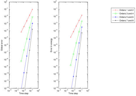
Figure 5: Global errors for the rigid body simulations after $5$ seconds, HJ method.

The next figures show the nice behavior of the energy for the orders $2$, $4$, $6$ and $8$, for $h=0.05$. In the first three cases the behavior is essentially periodic, while in the last case the roundoff errors dominate and the evolution of the energy becomes a random walk.

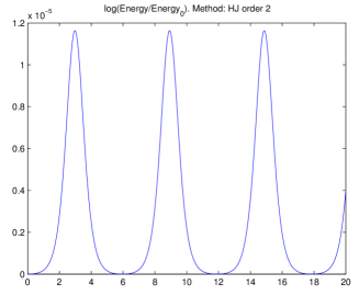
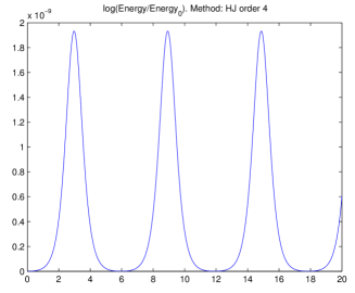
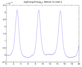
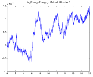
Figure 6: Energy conservation for the HJ method.

Notice that here we simulated the first $20$ seconds of the system, but the behavior of the energy is very stable, i.e., the energy seems to oscillate periodically for all time, as shown in Figure 7 where the first $25000$ seconds are simulated for the order $2$ method.

Figure 7: Long time energy conservation, order $2$ HJ method.

The Casimirs have an exceptional conservation even for order $2$ methods, as shown in the figures below.

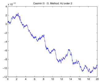
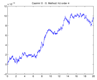
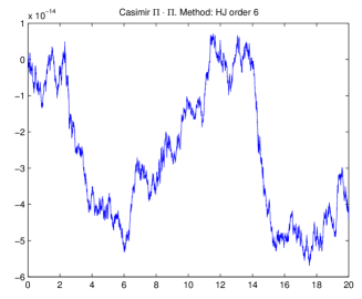
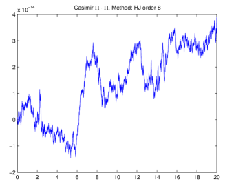
Figure 8: Casimir conservation, HJ method.

Compared to order $4$ Runge-Kutta, we observe that while the solution of our method oscillates periodically the Runge-Kutta method will get a bigger energy error after around $1000$ seconds.

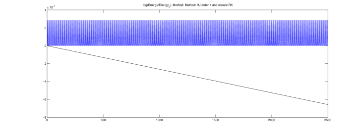
Figure 9: Energy conservation comparison. Order $4$ Runge-Kutta (below), and order $4$ HJ (above). $T=50$, $N=1000$, $h=T/N=0.05$.

We show the exceptional conservation of the Casimir for long time of our methods in the figure below, where we simulated the rigid body for $25000$ seconds.

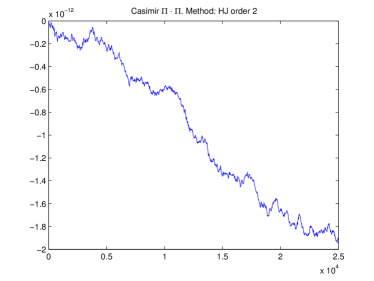
Figure 10: Casimir conservation, HJ order 2

5.2.2 Heavy Top

As a concrete example of a system evolving on a transformation Lie algebroid we consider the heavy top. This example is modeled on the action algebroid $\tau\ \colon\ S^{2}\times\mathfrak{so}(3)\to S^{2}$ with Hamiltonian

$$H(\Gamma,\Pi)=\frac{1}{2}\Pi\cdot I^{-1}\Pi+mgl\Gamma\cdot\mathbf{e},$$

where $\Pi\in\mathbb{R}^{3}\simeq\mathfrak{so}^{*}(3)$ is the angular momentum, $\Gamma$ is the direction opposite to the gravity and $\mathbf{e}$ is a unit vector in the direction from the fixed point to the center of mass, all of them expressed in a frame fixed to the body. The constants $m$, $g$ and $l$ are respectively the mass of the body, the strength of the gravitational acceleration and the distance from the fixed point to the center of mass. The matrix $I$ is the inertia tensor of the body (see [39, 46]). In this case the Lie groupoid under consideration, $G$, is the action groupoid $S^{2}\times SO(3)$, whose Lie algebroid is $S^{2}\times\mathfrak{so}(3)$. The source and target maps are given by

$$\begin{array}[]{c}\tilde{\alpha}_{\operatorname{cay}}(a_{1},a_{2},a_{3},x,y,z,p_{a_{1}},p_{a_{2}},p_{a_{3}},p_{x},p_{y},p_{z})\\ \vskip 6.0pt plus 2.0pt minus 2.0pt\cr=\left(\begin{array}[]{c}{a_{1}}\\ {a_{2}}\\ {a_{3}}\\ \left(\frac{{x}^{2}}{4}+1\right){p_{x}}+\left(\frac{xy}{4}-\frac{z}{2}\right){p_{y}}+\left(\frac{xz}{4}+\frac{y}{2}\right){p_{z}}+a_{2}p_{a_{3}}-a_{3}p_{a_{2}}\\ \left(\frac{xy}{4}+\frac{z}{2}\right){p_{x}}+\left(\frac{y^{2}}{4}+1\right){p_{y}}+\left(\frac{yz}{4}-\frac{x}{2}\right){p_{z}}-a_{1}p_{a_{3}}+a_{3}p_{a_{1}}\\ \left(\frac{xz}{4}-\frac{y}{2}\right){p_{x}}+\left(\frac{yz}{4}+\frac{x}{2}\right){p_{y}}+\left(\frac{z^{2}}{4}+1\right){p_{z}}+a_{1}p_{a_{2}}-a_{2}p_{a_{1}}\end{array}\right)\\ \vskip 6.0pt plus 2.0pt minus 2.0pt\cr\textrm{and}\\ \vskip 6.0pt plus 2.0pt minus 2.0pt\cr\tilde{\beta}_{\operatorname{cay}}(a_{1},a_{2},a_{3},x,y,z,p_{a_{1}},p_{a_{2}},p_{a_{3}},p_{x},p_{y},p_{z})\\ \vskip 6.0pt plus 2.0pt minus 2.0pt\cr=\left(\begin{array}[]{c}{\frac{\left({x}^{2}-{y}^{2}-{z}^{2}+4\right){a_{1}}}{{x}^{2}+{y}^{2}+{z}^{2}+4}}+{\frac{\left(2\,yx+4\,z\right){a_{2}}}{{x}^{2}+{y}^{2}+{z}^{2}+4}}+{\frac{\left(2\,zx-4\,y\right){a_{3}}}{{x}^{2}+{y}^{2}+{z}^{2}+4}}\\ {\frac{\left(2\,yx-4\,z\right){a_{1}}}{{x}^{2}+{y}^{2}+{z}^{2}+4}}+{\frac{\left(-{x}^{2}+{y}^{2}-{z}^{2}+4\right){a_{2}}}{{x}^{2}+{y}^{2}+{z}^{2}+4}}+{\frac{\left(2\,zy+4\,x\right){a_{3}}}{{x}^{2}+{y}^{2}+{z}^{2}+4}}\\ {\frac{\left(2\,zx+4\,y\right){a_{1}}}{{x}^{2}+{y}^{2}+{z}^{2}+4}}+{\frac{\left(2\,zy-4\,x\right){a_{2}}}{{x}^{2}+{y}^{2}+{z}^{2}+4}}+{\frac{\left(-{x}^{2}-{y}^{2}+{z}^{2}+4\right){a_{3}}}{{x}^{2}+{y}^{2}+{z}^{2}+4}}\\ \left(\frac{x^{2}}{4}+1\right){p_{x}}+\left(\frac{xy}{4}+\frac{z}{2}\right){p_{y}}+\left(\frac{xz}{4}-\frac{y}{2}\right){p_{z}}\\ \left(\frac{xy}{4}-\frac{z}{2}\right){p_{x}}+\left(\frac{y^{2}}{4}+1\right){p_{y}}+\left(\frac{yz}{4}+\frac{x}{2}\right){p_{z}}\\ \left(\frac{xz}{4}+\frac{y}{2}\right){p_{x}}+\left(\frac{yz}{4}-\frac{x}{2}\right){p_{y}}+\left(\frac{z^{2}}{4}+1\right){p_{z}}\end{array}\right)\end{array}$$

We have run simulations using truncations of $S$ up to order 8 and the results are collected in Figure 11. The initial condition was $\left(\Gamma_{0},\Pi_{0})=((0.5,0.5,-0.5)/\|(0.5,0.5,-0.5)\|,(0.1,-1,2)\right)$ and the parameters were $I=\operatorname{diag}(1,1.5,2)$, $m=0.1$, $g=9.8$, $l=0.2$ and $e=(0.1,0.2,0.5)/\|(0.1,0.2,0.5)\|$.

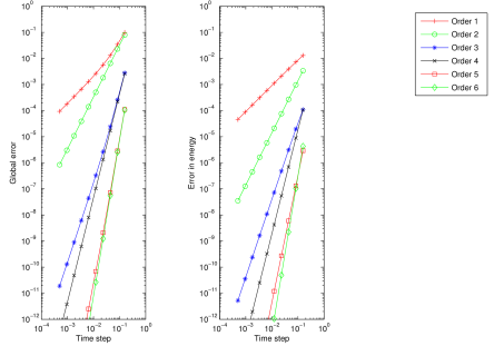
Figure 11: Global errors for the heavy top simulations, HJ method.

A similar behavior in the conservation of energy is observed.

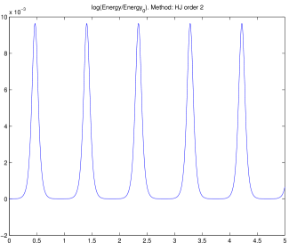
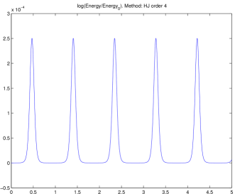
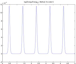
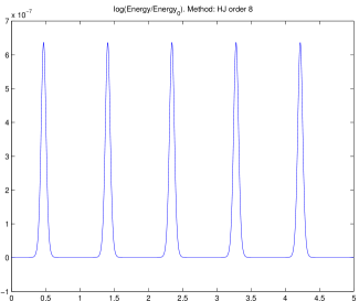
Figure 12: Energy conservation, HJ method.

The comparison with other non-geometric methods shows again a drift for the conservation of Casimirs and energy. See the figure below for a comparison of the conservation of Casimirs for the Hamilton-Jacobi and ode45 methods for the first $500$ seconds.

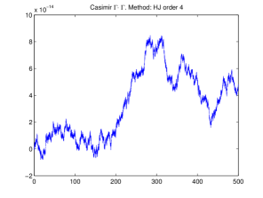
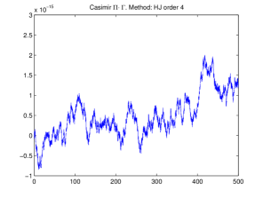
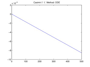
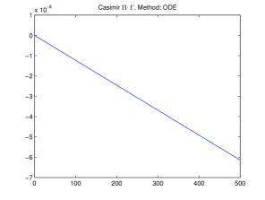
Figure 13: Casimir conservation. Comparison of HJ and ode45 methods.

5.2.3 Elroy’s Beanie

This system evolves on an Atiyah algebroid. It is probably the simplest example of a dynamical system with a non-Abelian Lie group of symmetries. It consists of two planar rigid bodies attached at their centers of mass, moving freely in the plane. The configuration space is $Q=SE(2)\times S^{1}$ with coordinates $(x,y,\theta,\psi)$, where the first three coordinates describe the position and orientation of the center of mass of the first body. The last one is the relative orientation between both bodies. The dynamics is determined by the Euler-Lagrange equations corresponding to the Lagrangian

$$L(x,y,\theta,\psi,\dot{x},\dot{y},\dot{\theta},\dot{\psi})=\frac{1}{2}m(\dot{x}^{2}+\dot{y}^{2})+\frac{1}{2}I_{1}\dot{\theta}^{2}+\frac{1}{2}I_{2}(\dot{\theta}+\dot{\psi})^{2}-V(\psi),$$

where $m$ denotes the mass of the system and $I_{1}$ and $I_{2}$ are the inertias of the first and the second body, respectively; additionally, we also consider a potential function of the form $V(\psi)$. This Lagrangian is $SE(2)$-invariant where the group action is given by:

$$\Phi_{g}(q)=\left(\begin{array}[]{c }z_{1}+x\cos\alpha-y\sin\alpha\\ z_{2}+x\sin\alpha+y\cos\alpha\\ \alpha+\theta\\ \psi\end{array}\right)$$

with $g=(z_{1},z_{2},\alpha)$ and $q=(x,y,\theta,\psi)$.

The Lie algebra ${\mathfrak{s}e}(2)$ is generated by matrices of the form

$$\hat{\xi}=\left(\begin{array}[]{ccc}0&\xi_{3}&\xi_{1}\\ -\xi_{3}&0&\xi_{2}\\ 0&0&0\end{array}\right)$$

with basis

$$e_{1}=\left(\begin{array}[]{ccc}0&0&1\\ 0&0&0\\ 0&0&0\end{array}\right),\qquad e_{2}=\left(\begin{array}[]{ccc}0&0&0\\ 0&0&1\\ 0&0&0\end{array}\right)\qquad\textrm{ and }e_{3}=\left(\begin{array}[]{ccc}0&1&0\\ -1&0&0\\ 0&0&0\end{array}\right).$$

Then, any $\xi\in{\mathfrak{se}(2)}$ is expressed as $\hat{\xi}=\xi_{1}e_{1}+\xi_{2}e_{2}+\xi_{3}e_{3}$ and the Lie algebra structure on ${\mathfrak{s}e}(2)$ is determined by

$$[e_{1},e_{2}]=0,\qquad[e_{1},e_{3}]=e_{2},\qquad[e_{2},e_{3}]=-e_{1}.$$

The quotient space $M=Q/G=(SE(2)\times S^{1})/SE(2)\simeq S^{1}$ is naturally parameterized by the coordinate $\psi$. The projection $\pi:Q\longrightarrow M$ is given in coordinates by $\pi(x,y,\theta,\psi)=\psi$, $TQ/G\simeq TS^{1}\times{\mathfrak{se}(2)}$ and the reduced Lagrangian reads

$$\mathfrak{l}(\psi,\dot{\psi},\xi_{1},\xi_{2},\xi_{3})=\frac{1}{2}m(\xi_{1}^{2}+\xi_{2}^{2})+\frac{1}{2}I_{1}\xi_{3}^{2}+\frac{1}{2}I_{2}(\xi_{3}+\dot{\psi})^{2}-V(\psi).$$

The reduced equations (Lagrange-Poincaré equations) are

$$\dot{\xi}_{1} =-\xi_{2}\xi_{3},$$

$$\dot{\xi}_{2} =\xi_{1}\xi_{3},$$

$$(I_{1}+I_{2})\dot{\xi}_{3}+I_{2}\ddot{\psi} =0,$$

$$I_{2}(\dot{\xi}_{3}+\ddot{\psi}) =-\displaystyle{\frac{\partial V}{\partial\psi}}.$$

The Hamiltonian framework is defined on $T^{*}Q/G\equiv T^{*}S^{1}\times{\mathfrak{s}e}^{*}(2)$ with coordinates $(\psi,p_{\psi};p_{1},p_{2},p_{3})$. The linear Poisson bracket is given by:

$$\{p_{1},p_{2}\}=0,\quad\{p_{1},p_{3}\}=-p_{2},\quad\{p_{2},p_{3}\}=p_{1},\quad\{p_{i},p_{\psi}\}=\{p_{i},\psi\}=0,\quad\{\psi,p_{\psi}\}=1$$

and the corresponding Hamiltonian function is

$$H(\psi,p_{\psi};p_{1},p_{2},p_{3})=\frac{1}{2m}\left({p_{1}}^{2}+p_{2}^{2}\right)+\frac{1}{2I_{2}}p_{\psi}^{2}+\frac{1}{2I_{1}}(p_{3}-p_{\psi})^{2}+V(\psi),$$

Using the Poisson structure and the Hamiltonian function, one can easily compute the Hamilton’s equations

$$\dot{p}_{1} =-\frac{p_{3}-p_{\psi}}{I_{1}}p_{2},$$

$$\dot{p}_{2} =\frac{p_{3}-p_{\psi}}{I_{1}}p_{1},$$

$$\dot{p}_{3} =0,$$

$$\dot{p}_{\psi} =-\displaystyle{\frac{\partial V}{\partial\psi}},$$

$$\dot{\psi} =\frac{p_{\psi}}{I_{2}}-\frac{p_{3}-p_{\psi}}{I_{1}}.$$

Now, to apply our Hamilton-Jacobi formalism, observe that $(Q\times Q)/G\simeq S^{1}\times S^{1}\times SE(2)$ and therefore $T^{*}(Q\times Q)/G)\simeq T^{*}S^{1}\times T^{*}S^{1}\times T^{*}SE(2)$. We compute the source and target map of the symplectic groupoid $\tilde{\alpha}:T^{*}S^{1}\times T^{*}S^{1}\times T^{*}SE(2)\rightarrow T^{*}S^{1}\times{\mathfrak{s}e}^{*}(2)$ and $\tilde{\beta}:T^{*}S^{1}\times T^{*}S^{1}\times T^{*}SE(2)\rightarrow T^{*}S^{1}\times{\mathfrak{s}e}^{*}(2)$

$$\begin{array}[]{l}\tilde{\alpha}(\psi_{1},p_{\psi}^{1},\psi_{2},p_{\psi}^{2},(z_{1},z_{2},\theta),P_{1},P_{2},P_{3})=(\psi_{1},-p_{\psi}^{1};P_{1},P_{2},P_{3}-P_{1}z_{2}+P_{2}z_{1}),\\ \vskip 6.0pt plus 2.0pt minus 2.0pt\cr\tilde{\beta}(\psi_{1},p_{\psi}^{1},\psi_{2},p_{\psi}^{2},(z_{1},z_{2},\theta),P_{1},P_{2},P_{3})=(\psi_{2},p_{\psi}^{2};P_{1}\cos\theta+P_{2}\sin\theta,-P_{1}\sin\theta+P_{2}\cos\theta,P_{3}).\end{array}$$

Therefore, the Hamilton-Jacobi equation is

$$\frac{\partial S}{\partial t}(t,p^{1}_{\psi},\psi_{2},p_{x},p_{y},p_{z})+\hat{H}(\frac{\partial S}{\partial p_{\psi}},-p_{\psi}^{1},\psi_{2},\frac{\partial S}{\partial\psi_{2}};\frac{\partial S}{\partial P_{1}},\frac{\partial S}{\partial P_{2}},\frac{\partial S}{\partial P_{3}},P_{1},P_{2},P_{3})=0$$

where $\hat{H}=H\circ\tilde{\beta}$

$$\hat{H}(\psi_{1},p_{\psi}^{1},\psi_{2},p_{\psi}^{2},z_{1},z_{2},\theta,P_{1},P_{2},P_{3}) = \frac{1}{2m}\left(({P_{1}\cos\theta+P_{2}\sin\theta})^{2}+(-P_{1}\sin\theta+P_{2}\cos\theta)^{2}\right)$$

$$+\frac{1}{2I_{2}}(p^{2}_{\psi})^{2}+\frac{1}{2I_{1}}(P_{3}-p^{2}_{\psi})^{2}.$$

The method was implemented numerically using $m=3$, $I_{1}=5$, $I_{2}=1$, with $T=10$ and several time step values. The potential energy is $V(\psi)=\cos(2\psi)$, and the initial conditions are $(\psi,p_{\psi},p_{1},p_{2},p_{3})=(1,-0.1,0.1,0.2,1)$. Figure 14 shows the global errors.

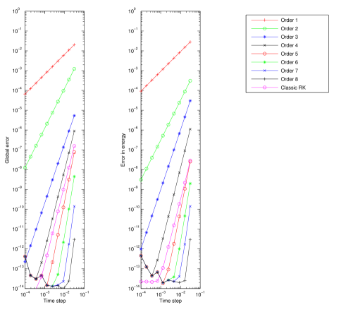
Figure 14: Global errors for the Elroy’s beanie simulations, HJ method.

Next, we show the energy error for different orders of our Hamilton-Jacobi method, for $N=1000$.

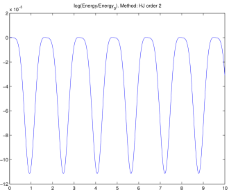
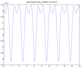
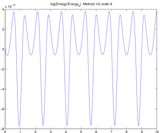
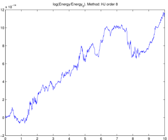
Figure 15: Energy conservation, HJ method.

Similar behavior to the previous cases can be observed. While for “short” times the behavior is similar to Runge-Kutta methods (of the same order) the exceptional energy and Casimir conservation should make our methods very well suited to study long term situations, which are of huge importance to study, for instance, invariant submanifolds (see below for the Runge Kutta’s energy drift). Some improvements of these methods, see next section, should provide means to understand the dynamics of more complicated systems.

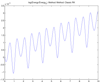
Figure 16: Energy conservation, Runge Kutta method.

6 Conclusions and Remarks

In this paper we developed a Hamilton–Jacobi theory for certain class of linear Poisson structures which happen to be general enough to include the systems important for classical mechanics. As a practical application we present an improvement of some Poisson numerical methods, previously introduced by Channell, Ge, Marsden and Scovel among others. There are still several issues to be exploited, we list some of them below.

1. Simplification of the Hamilton–Jacobi equations using Casimirs: In this paper we only treated some numerical methods as examples, but it is our belief that applications of our results are very promising for analytic integration of Hamilton’s equations. This should not be surprising, as the classical Hamilton–Jacobi theory has proved to be one of the most powerful tools for analytic integration, see Arnold’s quote in Section 1. In this regard, Casimirs should play an important role, based on the following observation. If $H:A^{*}G\rightarrow\mathbb{R}$ is the Hamiltonian under consideration, and $C:A^{*}G\rightarrow\mathbb{R}$ is a Casimir, then $X_{H}=X_{H+\lambda C}$, where $\lambda$ is a constant. Nonetheless, the Hamilton–Jacobi equations for $H$ and for $H+\lambda C$ could be very different. As a simple but illustrative application of this fact, we present here an application to the computation of the rigid body when two moments of inertia are equal. It is remarkable that in [49] the author uses a similar procedure to obtain explicit Lie–Poisson integrators. For more information about that relation see point 3 below.

   Example 2.

   Let $G$ be the Lie group $SO(3)$ and $0<\varphi<2\pi,\ 0<\theta<\pi,\ 0<\psi<2\pi$ be the Euler angles, defined following [45]. They form a coordinate chart, although not including the identity. The source and target of the cotangent groupoid read in the associated cotangent coordinates

   $$\begin{array}[]{l}\tilde{\alpha}(\varphi,\psi,\theta,p_{\varphi},p_{\psi},p_{\theta})\rightarrow\left(\begin{array}[]{c}\Pi_{1}=(((p_{\psi}-\cos(\theta)p_{\varphi})\sin(\varphi)+\cos(\varphi)\sin(\theta)p_{\theta})/\sin(\theta)\\ \Pi_{2}=((\cos(\theta)p_{\varphi}-p_{\psi})\cos(\varphi)+\sin(\theta)\sin(\varphi)p_{\theta})/\sin(\theta)\\ \Pi_{3}=p_{\varphi}\end{array}\right),\par\\ \vskip 12.0pt plus 4.0pt minus 4.0pt\cr\tilde{\beta}(\varphi,\psi,\theta,p_{\varphi},p_{\psi},p_{\theta})\rightarrow\left(\begin{array}[]{c}\Pi_{1}=((p_{\varphi}-p_{\psi}\cos(\theta))\sin(\psi)+p_{\theta}\sin(\theta)\cos(\psi))/\sin(\theta)\\ \Pi_{2}=((p_{\varphi}-p_{\psi}\cos(\theta))\cos(\psi)-p_{\theta}\sin(\theta)\sin(\psi))/\sin(\theta)\\ \Pi_{3}=p_{\psi}\end{array}\right).\par\end{array}$$

   The Lagrangian submanifold

   $$\mathcal{L}=\{(\pi,\pi/2,\pi/2,p_{\varphi},p_{\psi},p_{\theta})\textrm{ such that }p_{\varphi},\ p_{\psi},\ p_{\theta}\in\mathbb{R}\}$$

   generates the trasformation described by

   $$\begin{array}[]{c}\tilde{\alpha}(\pi,\pi/2,\pi/2,p_{\varphi},p_{\psi},p_{\theta})=(-p_{\theta},p_{\psi},p_{\varphi}),\par\\ \vskip 6.0pt plus 2.0pt minus 2.0pt\cr\tilde{\beta}(\pi,\pi/2,\pi/2,p_{\varphi},p_{\psi},p_{\theta})=(p_{\varphi},-p_{\theta},p_{\psi}),\end{array}$$

   that is,

   $$\hat{\mathcal{L}}(\Pi_{1},\Pi_{2},\Pi_{3})=(\Pi_{3},\Pi_{1},\Pi_{2}).$$

   This transformation is not the identity, due to problems with the parametrization of the identity using Euler’s angles, but it is a very easy transformation and invertible in a trivial way. Thus, it can be used instead of the identity transfomation to achieve analogous results. Following our previous construction we can give the generating function

   $$S(p_{\varphi},p_{\psi},p_{\theta})=\pi p_{\varphi}+(1/2)\pi p_{\psi}+(1/2)\pi p_{\theta}.$$

   The Hamiltonian of the rigid body dynamics, when two moments of inertia are equal, and the Casimir are given by

   $$\begin{array}[]{l}H(\Pi_{1},\Pi_{2},\Pi_{3})=\displaystyle\frac{1}{2}\left(\frac{\Pi_{1}^{2}}{I}+\frac{\Pi_{2}^{2}}{I}+\frac{\Pi_{3}^{2}}{I^{\prime}}\right),\\ \vskip 12.0pt plus 4.0pt minus 4.0pt\cr C(\Pi_{1},\Pi_{2},\Pi_{3})=\Pi_{1}^{2}+\Pi_{2}^{2}+\Pi_{3}^{2}.\end{array}$$

   The dynamics of the Hamiltonians $H$ and $H^{\prime}=H+\displaystyle\frac{1}{2I}C$ are equal, since $C$ is a Casimir

   $$X_{H^{\prime}}(\Pi_{1},\Pi_{2},\Pi_{3})=\left(\displaystyle\frac{I-I^{\prime}}{II^{\prime}}\Pi_{2}\Pi_{3}\right)\partial\Pi_{1}+\left(\displaystyle\frac{I^{\prime}-I}{II^{\prime}}\Pi_{1}\Pi_{3}\right)\partial\Pi_{2}+0\partial\Pi_{3}.$$

   Nonetheless, the Hamiltonians $H$ and $H^{\prime}$ are very different as functions, that implies that their $\tilde{\beta}$-pullback are quite disparate as well

   $$\begin{array}[]{rl}H\circ\tilde{\beta}&=\displaystyle\frac{1}{2}\left(\frac{[(p_{\varphi}-p_{\psi}\cos(\theta))\sin(\psi)+p_{\theta}\sin(\theta)\cos(\psi)]^{2}}{I\sin^{2}(\theta)}\right.\\ \vskip 6.0pt plus 2.0pt minus 2.0pt\cr&+\displaystyle\frac{[(p_{\varphi}-p_{\psi}\cos(\theta))\cos(\psi)+p_{\theta}\sin(\theta)\sin(\psi)]^{2}}{I\sin^{2}(\theta)}\par+\displaystyle\left.\frac{p_{\psi}^{2}}{I^{\prime}}\right)\end{array}$$

   while

   $$\begin{array}[]{rl}H^{\prime}\circ\tilde{\beta}&=\left(\displaystyle\frac{I-I^{\prime}}{II^{\prime}}\right){p_{\psi}^{2}}.\end{array}$$

   This fact should have implications in our Hamilton–Jacobi theory, and this is the case as we are going to show. A solution of the Hamilton–Jacobi equation using the Hamiltonian $H^{\prime}$

   $$\begin{array}[]{c}\displaystyle\frac{\partial S}{\partial t}(p_{\varphi},p_{\psi},p_{\theta})+(H^{\prime}\circ\tilde{\beta})(\frac{\partial S}{\partial p_{\varphi}},\frac{\partial S}{\partial p_{\psi}},\frac{\partial S}{\partial p_{\theta}},p_{\varphi},p_{\psi},p_{\theta})=0\\ \vskip 6.0pt plus 2.0pt minus 2.0pt\cr\Leftrightarrow\displaystyle\frac{\partial S}{\partial t}(p_{\varphi},p_{\psi},p_{\theta})+\left(\displaystyle\frac{I-I^{\prime}}{II^{\prime}}\right){p_{\psi}^{2}}=0\end{array}$$

   is given by direct inspection

   $$S(t,p_{\varphi},p_{\psi},p_{\theta})=-\left(\displaystyle\frac{I-I^{\prime}}{II^{\prime}}\right){p_{\psi}^{2}}t+S_{0}(p_{\varphi},p_{\psi},p_{\theta}),$$

   where $S_{0}$ is the initial condition, which is fixed to get the identity, so finally

   $$S(t,p_{\varphi},p_{\psi},p_{\theta})=-\left(\displaystyle\frac{I-I^{\prime}}{II^{\prime}}\right){p_{\psi}^{2}}t+\pi p_{\varphi}+(1/2)\pi p_{\psi}+(1/2)\pi p_{\theta}.$$

   For the sake of simplicity we chose to integrate the easiest term of the Hamiltonian, but the other terms are solvable in a similar fashion. On the other hand, the Hamilton–Jacobi equation for the Hamiltonian $H$ does not seem to be solvable in an obvious way. Although very elementary, this example shows that Casimirs can be used to simplify the Hamilton–Jacobi equation. A systematic development of these ideas should provide means to integrate the Hamilton–Jacobi equation. These ideas are exclusive of the Poisson setting, as the Casimirs are trivial for symplectic structures.

2. Improvement of the numerical methods: The numerical methods that we present here are very general and conserve the geometry very well, but they are not very efficient from the computational viewpoint. Our aim in this paper was to show how to use our results, rather than giving optimized numerical methods. Nonetheless, there is still a lot of room to improve these methods, as it has already been shown in [6, 13, 22, 38, 51] in the symplectic and Lie–Poisson case, where they give recipes to construct higher order approximations and reduce the computational cost. Those improvements can be applied in a straightforward fashion to our setting.

3. Ruth type integrators: Our methods are, generally, implicit. But in particular examples they can be made explicit sometimes. That is very important in order to develop very efficient methods, a nice exposition of these topics is given in [49] . This is a classical fact, as it happens already in the symplectic case, classical references are [26, 57] where the authors develop fourth order explicit methods for mechanical Hamiltonians, that is, of the form kinetic plus potential energy. Our approach seems to be useful in that regard. For instance, consider the example introduced in 1 and assume that the moments of inertia of the rigid body are different, so the Hamiltonian reads,

   $$H(\Pi_{1},\Pi_{2},\Pi_{3})=\displaystyle\frac{1}{2}\left(\frac{\Pi_{1}^{2}}{I^{1}}+\frac{\Pi_{2}^{2}}{I^{2}}+\frac{\Pi_{3}^{2}}{I^{3}}\right).$$

   We can use the Casimir to simplify one of the terms without changing the dynamics,

   $$H^{\prime}=H-\displaystyle\frac{1}{2I^{1}}C=\frac{1}{2}\left(\frac{I^{1}-I^{2}}{I^{1}I^{2}}\Pi_{2}^{2}+\frac{I^{1}-I^{3}}{I^{1}I^{3}}\Pi_{3}^{2}\right)=C^{1}\Pi^{2}_{2}+C^{2}\Pi^{2}_{3},$$

   where $C^{1}=\displaystyle\frac{I^{1}-I^{2}}{2I^{1}I^{2}}$ and $C^{2}=\displaystyle\frac{I^{1}-I^{3}}{2I^{1}I^{3}}$. And using the previous expression for $\tilde{\beta}$ we get

   $$H^{\prime}\circ\tilde{\beta}=C^{1}\left(\displaystyle\frac{[(p_{\varphi}-p_{\psi}\cos(\theta))\cos(\psi)+p_{\theta}\sin(\theta)\sin(\psi)]^{2}}{\sin^{2}(\theta)}\right)+C^{2}p_{\psi}^{2}$$

   and the Hamilton–Jacobi equation becomes

   $$\frac{\partial S}{\partial t}+C^{1}\left(\displaystyle\frac{[(p_{\varphi}-p_{\psi}\cos(\frac{\partial S}{\partial p_{\theta}}))\cos(\frac{\partial S}{\partial p_{\psi}})+p_{\theta}\sin(\frac{\partial S}{\partial p_{\theta}})\sin(\frac{\partial S}{\partial p_{\psi}})]^{2}}{\sin^{2}(\frac{\partial S}{\partial p_{\theta}})}\right)+C^{2}(\frac{\partial S}{\partial p_{\psi}})^{2}=0.$$

   This equation is not easily integrable, but clearly $H=H^{1}+H^{2}$ where

   $$\begin{array}[]{rl}H^{1}&=C^{1}\left(\displaystyle\frac{[(p_{\varphi}-p_{\psi}\cos(\theta))\cos(\psi)+p_{\theta}\sin(\theta)\sin(\psi)]^{2}}{\sin^{2}(\theta)}\right)\\ \vskip 12.0pt plus 4.0pt minus 4.0pt\cr H^{2}&=C^{2}p_{\psi}^{2}\end{array}$$

   and the Hamilton–Jacobi equation for each of the Hamiltonians is easily solvable by

   $$\begin{array}[]{rl}S^{1}(t,p_{\varphi},p_{\psi},p_{\theta})&=-C^{1}{p_{\theta}^{2}}t+\pi p_{\varphi}+(1/2)\pi p_{\psi}+(1/2)\pi p_{\theta},\\ \vskip 6.0pt plus 2.0pt minus 2.0pt\cr\textrm{and}\\ \vskip 6.0pt plus 2.0pt minus 2.0pt\cr S^{2}(t,p_{\varphi},p_{\psi},p_{\theta})&=-C^{2}p_{\psi}^{2}t+\pi p_{\varphi}+(1/2)\pi p_{\psi}+(1/2)\pi p_{\theta},\end{array}$$

   respectively. Each of the solutions gives an explicit transformation which is a rotation. The composition of the explicit transformations induced by $S^{1}$ and $S^{2}$ gives the method introduced by R.I. McLachlan in [49], but we obtained it from the Hamilton–Jacobi theory. The development of a rigorous Ruth type integration techniques will provide very efficient numerical methods which conserve the geometry. We want to stress here that all the theoretical tools used in [26, 57]: the change of the Hamiltonian under a canonical transformation, the different types of generating functions,… were already introduced in this work. These results applied to the linear Poisson setting were not present in the literature until now, as far as we know. The importance of the groupoid setting was already noticed by C. Scovel and A.D. Weinstein. We recall the quote from [59], “The groupoid aspect of the theory also provides natural Poisson maps, useful in the application of Ruth type integration techniques, which do not seem easily derivable from the general theory of Poisson reduction”.

4. Reduction of the Hamilton–Jacobi equation: Some of the authors of this paper developed a reduction and reconstruction procedure for the Hamilton–Jacobi equation, see [20], based on the following lemma (see [20, 27]).

   Lemma 9.

   Let $(M,\Omega)$ a symplectic manifold, $G$ a connected Lie group and $\Phi:G\times M\rightarrow M$ an action by symplectomorphisms. Assume that this action has an equivariant momentum mapping, say $J:M\rightarrow\mathfrak{g}^{*}$. Given a (connected) Lagrangian submanifold $\mathcal{L}\subset M$, the following conditions are equivalent:

   1. $\mathcal{L}$ is a $G$-invariant Lagrangian submanifold,

   2. $J_{|\mathcal{L}}=\mu$, i.e., $J$ is constant on $\mathcal{L}$.

   The results introduced recently in [23] should permit the development of a reduction theory applicable to our framework. As an evidence of this fact, notice that in [23] the authors obtain a momentum mapping for an action which resembles the cotangent lifted actions. That setting is very similar to the one used by the authors in [20] and so it seems very likely to be that reduction theory applies to our theory.

   We also want to stress here that the reconstruction procedure introduced in the aforementioned work [20] can be combined with the Hamilton-Jacobi theory developed here to obtain symplectic integrators that conserve momentum mappings in the same way that Poisson integrators conserve the Casimirs.

5. The reduced Hamilton-Jacobi theory: a discrete principal connection approach. Let $H:T^{*}P\to\mathbb{R}$ be a Hamiltonian function which is invariant under the cotangent lift of a free and proper action of the Lie group $G$ on $P$. Denote by $M$ the space of orbits of the action of $G$ on $P$. Then, one may consider the reduced Hamiltonian function $H_{red}:T^{*}P/G\to\mathbb{R}$ and the corresponding Hamilton-Poincaré dynamics.

   Suppose that $S:\mathbb{R}\times(P\times P)/G\to\mathbb{R}$ is a solution of the Hamilton-Jacobi equation

   $$H_{red}^{ext}\circ dS=\beta_{\mathbb{R}}^{*}K,\;\;\mbox{ with }K:\mathbb{R}\times M\to\mathbb{R}.$$

   Note that the involved spaces in the previous equation are quotient manifolds. So, in order to write the Hamilton-Jacobi equation in a suitable way, we may use a discrete principal connection on the principal $G$-bundle $\pi:P\to M$ [24, 36, 39]. In fact, in the presence of a discrete principal connection, one obtains a decomposition of the tangent bundle to $\mathbb{R}\times(P\times P)/G$ as follows

   $$T(\mathbb{R}\times(P\times P)/G)\simeq T\mathbb{R}\oplus T(M\times M)\oplus T((P\times G)/G)$$

   Thus, the Hamilton-Jacobi equation

   $$d(H_{red}^{ext}\circ dS)=d(\beta_{\mathbb{R}}^{*}K)$$

   may be decomposed into the horizontal Hamilton-Jacobi equation and the vertical Hamilton-Jacobi equation. It would be interesting to check the efficiency of this method in some explicit examples of symmetric Hamiltonian systems. This will be the subject of a forthcoming paper. Anyway, the use of a (continuous) principal connection has proved to be a very useful method in the discussion of Hamilton-Poincaré (resp. Lagrange-Poincaré) equations associated with a symmetric Hamiltonian (resp. Lagrangian) system (see [11, 12, 43]). Even extensions of these methods for higher-order mechanical systems and for classical field theories have been also discussed in the literature (see [21, 28]).

6. Truncation of infinite-dimensional Poisson systems using linear Poisson structures: There are several examples of relevant physical importance which are infinite-dimensional Poisson systems: Euler equations of incompressible fluids, Vlasov–Maxwell and Vlasov–Poisson equations… Truncations of some of those systems conserving the geometry have already been carried out successfully [49, 59, 63, 64]. In this regard, it seems that linear Poisson structures, i.e. dual bundles of Lie algebroids, should be the natural setting for that. After that truncation is done, our methods could be applied in order to understand the qualitative behavior of those infinite-dimensional systems.

7. Poincaré’s generating function: Poincaré’s generating functions have been used in dynamical systems in order to relate critical points of a function to periodic orbits. Our setting admits an analogous theory using the coordinates introduced previously. We describe these statements in the Lie algebra case below.

   Example 3.

   Let $G$ be a Lie group with Lie algebra $\mathfrak{g}$. Consider $(g^{i},p_{i})$ a set of coordinates introduced following Section 3.6.2. Then the following lemma holds.

   Lemma 10.

   Let $S(p_{i})$ a function such that the corresponding Lagrangian submanifold $\{(\frac{\partial S}{\partial p_{i}},p_{i})/p_{i}\in\mathbb{R}\}$ is a bisection, and let $\hat{S}:\mathfrak{g}^{*}\rightarrow\mathfrak{g}^{*}$ be the induced Poisson transformation. Then the critical points of $S$ correspond to fixed points of $\hat{S}$.

   Proof.

   The Lagrangian submanifold that generates the identity is given in those coordinates by

   $$\mathcal{L}_{\operatorname{id}}=\{(0^{i},p_{i})\textrm{ such that }p_{i}\in\mathbb{R}\}$$

   and so $\mathcal{L}_{\operatorname{id}}\cap\textrm{graph}(dS)=\{\textrm{critical points of }S\}$ which concludes the proof. ∎

   Similar results can be obtained in the general situation.

8. Other geometric settings: Non-holonomic mechanics. In this paper we showed that, with the appropriate geometric tools, the classical complete solutions of the Hamilton–Jacobi theory can be extended to the Poisson case. This extension, far from being just a theoretical question, gives means to study Hamiltonian dynamical systems, numerically and analytically. Recently, the Hamilton-Jacobi theory has been extended to other frameworks, like the non-holonomic mechanics, see [10, 18, 54, 56]. Unfortunately, to the best of our knowledge, in the mentioned works there is not described a way to generate transformations from complete solutions of the Hamilton-Jacobi equation, analogous to the results described here. To obtain such a procedure will be extremely illuminating in order to construct non-holonomic integrators. Anyway, Hamilton–Jacobi theory for non-holonomic mechanical systems may be a useful method to obtain first integrals of the system [10, 33] which eventually will facilitate the integration of the systems. So, in conclusion, Hamilton–Jacobi theory could be used in the integration of some interesting symmetric non-holonomic systems which have been discussed, very recently, using new geometric tools (see [3, 4, 5]).

Appendix A Lie Algebroids

In this section we will recall the definition of a Lie algebroid (see [8, 37]). Associated to every Lie groupoid there is a Lie algebroid, as can be seen in Appendix B, although the converse is not true.

A.1 Definition

A Lie algebroid is a vector bundle $\tau:A\rightarrow M$ endowed with the following data:

• A bundle map $\rho:A\rightarrow TM$ called the anchor.

• A Lie bracket on the space of sections $\Gamma(\tau)$ satisfying the Leibniz identity, i.e.

  $$[\![X,fY]\!]=f[\![X,Y]\!]+\mathcal{L}_{\rho(X)}(f)Y$$

  for all $X,\ Y\in\Gamma(\tau)$ and any $f\in C^{\infty}(M)$.

A.2 Examples

In this section, we introduce some examples of Lie algebroids. More examples, maybe the most natural ones, will be sketched in Appendix B when we talk about the Lie algebroid associated with a Lie groupoid.

A.2.1 Vector Fields

It can be seen that given a manifold $M$ there is a one-to-one correspondence between Lie algebroid structures on the trivial bundle $M\times\mathbb{R}$ and vector fields $X$ on $M$. The vector bundle $\tau:A=M\times\mathbb{R}\rightarrow M$ is given just by the projection onto $M$.

1. The anchor map $\rho:A\rightarrow TM$ is given by $\rho(m,t)=tX(m)\in TM$.

2. Given $f,\ g\in C^{\infty}(M)$ then $[\![f,g]\!]=fX(g)-gX(f)$.

A.2.2 $2$-forms

Let $M$ be a manifold and consider now the bundle $A=TM\times\mathbb{R}$ over $M$, where the vector bundle structure $\tau:A\rightarrow M$ is the obvious one. Any closed $2$-form $\omega$ on $M$ defines a Lie algebroid estructure on that bundle:

1. The anchor $\rho:A\rightarrow TM$ is given by the projection onto the first factor.

2. The Lie bracket is given by $[\![(X,f),(Y,g)]\!]=([X,Y],\ X(g)-Y(f)+\omega(X,Y))$

Remark 26.

This case can be used to find examples of non-integrable Lie algebroids.

A.2.3 Poisson Manifolds

One really important example of Lie algebroids is given by Poisson manifolds. Let $(P,\Lambda)$ be a Poisson manifold, then we consider the cotangent bundle of $P$, $\pi_{P}:T^{*}P\rightarrow P$ and where the anchor and the Lie bracket are given by:

1. The anchor map is just the induced morphism $\Lambda^{\sharp}:T^{*}P\rightarrow TP$ by the Poisson tensor $\Lambda$.

2. The Lie bracket is given by $[\![\alpha,\beta]\!]=\mathcal{L}_{\Lambda^{\sharp}(\alpha)}\beta-\mathcal{L}_{\Lambda^{\sharp}(\beta)}\alpha-d(\Lambda(\alpha,\beta))$ for all $\alpha$ and $\beta$ $1$-forms on $P$.

A.3 The Poisson Structure of the Dual of a Lie Algebroid

Given a Lie algebroid $(\tau:A\rightarrow M,\ \rho,\ [\![\cdot{},\ \cdot{}]\!])$, its dual $A^{*}$ has a natural linear Poisson structure that we proceed to describe now.

Given $X$ and $Y$ sections of $\tau$, then they determine linear functions on $A^{*}$ that we denote by $\hat{X}$ and $\hat{Y}$. On the other hand each $f\in C^{\infty}(M)$ determines a function $f\circ\tau$ which is constant on the fibers. It can be seen that there exists a unique Poisson structure on $A^{*}$ which satisfies

$$\begin{array}[]{l}\{\hat{X},\hat{Y}\}=\widehat{[\![X,Y]\!]},\\ \vskip 6.0pt plus 2.0pt minus 2.0pt\cr\{\hat{X},f\circ\tau\}=(\rho(X)(f))\circ\tau,\\ \vskip 6.0pt plus 2.0pt minus 2.0pt\cr\{f\circ\tau,g\circ\tau\}=0,\end{array}$$

for all $X,Y\in\Gamma(\tau)$ and $f,g\in C^{\infty}(M)$.

Once we choose a local basis of sections $e_{j}$ $j=1,\ldots,m$ and local coordinates $x^{i}$ $i=1,\ldots,n$ on $M$. This system induces local coordinates in $A^{*}$ by $(x^{i},\mu_{i})$, where $i=1,\ldots,n$, $j=1,\ldots,m$ and where $\mu_{i}=\hat{e}_{i}$. If the structure functions and the anchor map read locally

$$[\![e_{i},e_{j}]\!]=c^{k}_{ij}e_{k}\quad\textrm{ and }\quad\rho(e_{i})=\rho^{j}_{i}\displaystyle\frac{\partial}{\partial x^{j}},$$

then the Poisson bracket on the coordinates $(x^{i},\mu_{j})$ reads

$$\begin{array}[]{c}\{x^{i},x^{j}\}=0,\\ \vskip 6.0pt plus 2.0pt minus 2.0pt\cr\{\mu_{i},x^{j}\}=\rho_{i}^{j},\\ \vskip 6.0pt plus 2.0pt minus 2.0pt\cr\{\mu_{i},\mu_{j}\}=c_{ij}^{k}\mu_{k}.\end{array}$$

Due to our conventions, this Poisson structure is the opposite to the one that makes $\tilde{\beta}$ a Poisson mapping. So in our work we are considering the Poisson structure $(A^{*}G,-\{\cdot{},\ \cdot{}\})$.

Appendix B Lie Groupoids

We recall here the definition of a (Lie) groupoid. For more information about this concept, we refer the reader to the monograph [17] and K. Mackenzie’s book [37].

B.1 Definition

Groupoids:

A groupoid is a set $G$ equipped with the following data:

1. another set $M$, called the base;

2. two surjective maps $\alpha\colon G\to M$ and $\beta\colon G\to M$, called, respectively, the source and target projections; we visualize an element $g\in G$ as an arrow from $\alpha(g)$ to $\beta(g)$:

3. A partial multiplication, or composition map, $m\colon G_{2}\to G$ defined on the subset $G_{2}$ of $G\times G$:

   $$G_{2}=\left\{(g,h)\in G\times G\mid\beta(g)=\alpha(h)\right\}.$$

   The multiplication will be denoted for simplicity by $m(g,h)=gh$. It verifies the following properties:

   1. $\alpha(gh)=\alpha(g)$ and $\beta(gh)=\beta(h)$.

   2. $(gh)k=g(hk)$.

4. An identity section $\epsilon\colon M\to G$ such that

   1. $\epsilon(\alpha(g))g=g$ and $g\epsilon(\beta(g))=g$ for all $g\in G$,

   2. $\alpha(\epsilon(x))=\beta(\epsilon(x))=x$ for all $x\in M$.

5. An inversion map $\iota\colon G\to G$, to be denoted simply by $\iota(g)=g^{-1}$, such that

   1. $g^{-1}g=\epsilon(\beta(g))$ and $gg^{-1}=\epsilon(\alpha(g))$.

We will denote a groupoid $G$ over a base $M$ by or simply $G\rightrightarrows M$.

It is easy to see that $\epsilon$ must be injective, so there is a natural identification between $M$ and $\epsilon(M)$. However, we will keep a distinction between the two sets.

Lie Groupoids:

A groupoid, $G\rightrightarrows M$, is said to be a Lie groupoid if $G$ and $M$ are differentiable manifolds, all the structural maps are differentiable and besides, $\alpha$ and $\beta$ differentiable submersions. If $G\rightrightarrows M$ is a Lie groupoid then $m$ is a submersion, $\epsilon$ is an embedding and $\iota$ is a diffeomorphism. Notice that since $\alpha$ and $\beta$ are submersions, the $\alpha$ and $\beta$-fibers are submanifolds. The same properties imply that $G_{2}$ is a submanifold. We will use $G^{x}=\alpha^{-1}(x)$, $G_{y}=\beta^{-1}(y)$ and $G^{x}_{y}=\alpha^{-1}(x)\cap\beta^{-1}(y)$.

Left and Right multiplication:

Given $g\in G_{y}^{x}$, so $g:x\to y$, we can define two (bijective) mappings $l_{g}\colon G^{y}\to G^{x}$ and and $r_{g}\colon G_{x}\to G_{y}$, which are the left translation by $g$ and the right translation by $g$ respectively. These diffeomorphisms are given by

$$\begin{array}[]{lcr}\begin{array}[]{rccl}l_{g}\colon&G^{y}&\longrightarrow&G^{x}\\ &h&\mapsto&l_{g}(h)=gh\end{array}&;&\begin{array}[]{rccl}r_{g}\colon&G_{x}&\longrightarrow&G_{y}\\ &h&\mapsto&r_{g}(h)=hg,\end{array}\end{array}$$ (33)

where we have that $(l_{g})^{-1}=l_{g^{-1}}$ and $(r_{g})^{-1}=r_{g^{-1}}$.

Bisections:

A submanifold $\mathcal{B}\subset G$ is called a bisection of $G$ if the restricted maps, $\alpha_{|\mathcal{B}}:\ \mathcal{B}\rightarrow M$ and $\beta_{|\mathcal{B}}:\ \mathcal{B}\rightarrow M$ are both diffeomorhisms. Consequently, for any bisection $\mathcal{B}\subset G$, there is a corresponding $\alpha$-section $\mathcal{B}_{\alpha}=(\alpha_{|\mathcal{B}})^{-1}:\ M\rightarrow\mathcal{B}$, where $\beta\circ\mathcal{B}_{\alpha}:\ M\rightarrow M$ is a diffeomorphism. Likewise, there is a $\beta$-section $\mathcal{B}_{\beta}=(\beta_{|\mathcal{B}})^{-1}:\ M\rightarrow G$, where $\alpha\circ\mathcal{B}_{\beta}=(\beta\circ\mathcal{B}_{\alpha})^{-1}:\ M\rightarrow M$ is a diffeomorphism. More generally, $\mathcal{B}\subset G$ is called a local bisection if the restricted maps $\alpha_{|\mathcal{B}}$ and $\beta_{|\mathcal{B}}$ are local diffeomorphisms onto open sets, $U,\ V\subset M$, respectively. Local bisections on a Lie groupoid always exist.

Invariant Vector Fields:

A vector field $X$ on $G$ is said to be left-invariant (resp., right-invariant) if it is tangent to the fibers of $\alpha$ (resp., $\beta$) and

$$X(gh)=(T_{h}l_{g})(X(h))\quad\Big{(}\textrm{ resp. }X(gh)=(T_{g}r_{h})(X(g))\Big{)}$$

for all $(g,h)\in G_{2}$.

Morphisms:

Given two Lie groupoids $G\rightrightarrows M$ and $G^{\prime}\rightrightarrows M^{\prime}$, a morphism of Lie groupoids is a smooth map $\Phi\colon G\to G^{\prime}$ such that

1. If $(g,h)\in G_{2}$ then $(\Phi(g),\Phi(h))\in(G^{\prime})_{2}$ and

2. $\Phi(gh)=\Phi(g)\Phi(h)$.

A morphism of Lie groupoids $\Phi\colon G\to G^{\prime}$ induces a smooth map $\Phi_{0}\colon M\to M^{\prime}$ in such a way that the source, the target and the identity section commute with the morphism, i.e.

$$\alpha^{\prime}\circ\Phi=\Phi_{0}\circ\alpha,\makebox[8.5359pt]{}\beta^{\prime}\circ\Phi=\Phi_{0}\circ\beta,\makebox[8.5359pt]{}\Phi\circ\epsilon=\epsilon^{\prime}\circ\Phi_{0},$$

$\alpha$, $\beta$ and $\epsilon$ (resp., $\alpha^{\prime}$, $\beta^{\prime}$ and $\epsilon^{\prime}$) being the source, the target and the identity sections of $G$ (resp., $G^{\prime}$).

B.2 Lie Algebroid Associated to a Lie Groupoid

Given a Lie groupoid $G$ we denote by $AG=\ker(T\alpha)_{|\epsilon(M)}$, i.e., the set of vectors tangent to the $\alpha$-fibers restricted to the units of the groupoid. Since the units, $\textrm{Im}(\epsilon)$, are diffeomorphic to the base manifold, $M$, we will consider the set $AG$ as a vector bundle $\tau\colon AG\to M$. The reader should keep this identification in mind, because it is going to be used implicitly in some places ($M\equiv\textrm{Im}(\epsilon)\subset G$).

It is easy to prove that there exists a bijection between the space of sections $\Gamma(\tau)$ and the set of left-invariant (resp., right-invariant) vector fields on $G$. If $X$ is a section of $\tau\colon AG\to M$, the corresponding left-invariant (resp., right-invariant) vector field on $G$ will be denoted $\overleftarrow{X}$ (resp., $\overrightarrow{X}$), where

$$\overleftarrow{X}(g)=(T_{\epsilon(\beta(g))}l_{g})(X(\beta(g))),$$ (34)

$$\left(\textrm{resp.,\ }\overrightarrow{X}(g)=-(T_{\epsilon(\alpha(g))}r_{g}\circ\iota)(X(\alpha(g)))\right),$$ (35)

for $g\in G$.

Using the above facts, we may introduce a Lie algebroid structure $([\![\cdot,\cdot]\!],\rho)$ on $AG$:

1. The anchor map $\rho\colon AG\to TM$ is

   $$\rho(X)(x)=(T_{\epsilon(x)}\beta)(X(x))$$

   for $X\in\Gamma(\tau)$ and $x\in M$.

2. The Lie bracket on the space of sections $\Gamma(\tau)$, denoted by $[\![\cdot,\cdot]\!]$ is defined by

   $$\overleftarrow{[\![X,Y]\!]}=[\overleftarrow{X},\overleftarrow{Y}],$$

   for $X,Y\in\Gamma(\tau)$ and $x\in M$.

   Note that

   $$\overrightarrow{[\![X,Y]\!]}=-[\overrightarrow{X},\overrightarrow{Y}],\makebox[8.5359pt]{}[\overrightarrow{X},\overleftarrow{Y}]=0,$$

   $$T\iota\circ\overrightarrow{X}=-\overleftarrow{X}\circ\iota,\;\;\;\;T\iota\circ\overleftarrow{X}=-\overrightarrow{X}\circ\iota,$$

   (for more details, see [37]). The dual bundle of $AG$ will be denoted by $A^{*}G$.

In addition, define the vector bundle $V\alpha$ as the sub-bundle of $TG$ consisting of $\alpha$-vertical vectors, that is, vectors tangent to the $\alpha$-fibers. $V\beta$ is defined analogously. Thus $AG$ is the restriction of $V\alpha$ to $\epsilon(M)$.

B.3 Examples of Lie groupoids

Next, we will present some examples of Lie groupoids. The corresponding associated Lie algebroid is pointed out in each case.

B.3.1 Lie Groups

Any Lie group $G$ is a Lie groupoid over $\{\mathfrak{e}\}$, the identity element of $G$.

1. The source, $\alpha$, is the constant map $\alpha(g)=\mathfrak{e}$.

2. The target, $\beta$, is the constant map $\beta(g)=\mathfrak{e}$.

3. The identity map is $\epsilon(\mathfrak{e})=\mathfrak{e}$.

4. The inversion map is $\iota(g)=g^{-1}$.

5. The multiplication is $m(g,h)=g\cdot h$, for any $g$ and $h$ in $G$.

Associated Lie algebroid:

The Lie algebroid associated with $G$ is just the Lie algebra ${\mathfrak{g}}$ of $G$ in a straightforward way.

B.3.2 The Pair or Banal Groupoid

Let $M$ be a manifold. The product manifold $M\times M$ is a Lie groupoid over $M$ called the pair or banal groupoid. Its structure mappings are:

1. The source, $\alpha$, is the projection onto the first factor.

2. The target, $\beta$, is the projection onto the second factor.

3. The identity map is $\epsilon(x)=(x,x)$, for all $x\in M$.

4. The inversion map is $\iota(x,y)=(y,x)$.

5. The multiplication is $m((x,y),(y,z))=(x,z)$, for $(x,y),(y,z)\in M\times M$.

Associated Lie Algebroid:

If $x$ is a point of $M$, it follows that

$$A=\ker(T\alpha)_{\epsilon(x)}=\{0_{x}\}\times T_{x}M$$

which gives the vector bundle structure and given $(0_{x},X_{x})\in A$, then

$$\tau(0_{x},X_{x})=x.$$

1. The anchor is given by the projection over the second factor $\rho(0_{x},X_{x})=X_{x}\in T_{x}M$

2. The Lie bracket on the space of sections, $\Gamma(\tau)$, is the Lie bracket of vector fields on the second factor $[\![(0,X),(0,Y)]\!]=(0,[X,Y])$.

In conclusion, we have that the Lie algebroid $A(Q\times Q)\to Q$ may be identified with the standard Lie algebroid $\tau_{Q}:TQ\to Q$.

B.3.3 Atiyah or Gauge Groupoids

Let $\pi\colon P\rightarrow M$ be a principal $G$-bundle. Then the free action $\Phi\colon G\times P\to P$ induces the diagonal action $\Phi^{\prime}\colon G\times(P\times P)\to P\times P$ by $\Phi^{\prime}(g,(q,q^{\prime}))=(gq,gq^{\prime})$. Moreover, one may consider the quotient manifold $(P\times P)/G$ and it admits a Lie groupoid structure over $M$, called the Atiyah or Gauge groupoid (see, for instance, [37, 39]). We describe now the structural mappings.

1. The source, ${\alpha}\colon(P\times P)/G\to M$ is given by $[(q,q^{\prime})]\mapsto\pi(q)$.

2. The target, ${\beta}\colon(P\times P)/G\to M$ is given by $[(q,q^{\prime})]\mapsto\pi(q^{\prime})$.

3. The identity map, ${\epsilon}\colon M\to(P\times P)/G$ is $x\mapsto[(q,q)],\;\mbox{ if }\pi(q)=x.$

4. The inversion map, ${\iota}\colon(P\times P)/G\to(P\times P)/G$ is $[(q,q^{\prime})]\mapsto[(q^{\prime},q)]$.

5. The multiplication map ${m}\colon((P\times P)/G)_{2}\to(P\times P)/G$ is $([(q,q^{\prime})],[(gq^{\prime},q^{\prime\prime})])\mapsto[(gq,q^{\prime\prime})]$.

Associated Lie Algebroid:

It easily follows that $A=\ker{T\alpha}_{\epsilon(M)}$ can be identified with $TP/G$. Then the associated Lie algebroid is just $\tau:TP/G\rightarrow M$, where $\tau$ is the obvious projection and the Lie algebroid structure is provided by

1. The anchor, $\rho:TP/G\rightarrow TM$, is given by the quotient of the natural projection map $T\pi:TP\rightarrow TM$. That is, $\rho=\tilde{T\pi}:TP/G\rightarrow TM$.

2. The space of sections of the vector bundle $\tau:TP/G\to P/G=M$ may be identified with the set of $G$-invariant vector fields on $P$. Under this identification, the Lie bracket on the space of sections is given by the standard Lie bracket of vector fields. We remark that it is easy to see that the Lie bracket of two $G$-invariant vector fields is another $G$-invariant vector field.

B.3.4 Action Lie groupoids

Let $G$ be a Lie group and let ${\Phi}\colon M\times G\to M$, $(x,g)\mapsto xg$, be a right action of $G$ on $M$. Consider the action Lie groupoid $M\times G$ over $M$ with structural maps given by

1. The source is ${\alpha}(x,g)=x$.

2. The target is ${\beta}(x,g)=xg$.

3. The identity map is ${\epsilon}(x)=(x,{e})$.

4. The inversion map is ${\iota}(x,g)=(xg,g^{-1})$.

5. The multiplication is $m((x,g),(xg,g^{\prime}))=(x,gg^{\prime})$.

See, for instance, [37, 39] for the details.

Associated Lie Algebroid:

Now, let ${\mathfrak{g}}=T_{{e}}G$ be the Lie algebra of $G$. Given $\xi\in\mathfrak{g}$ we will denote by $\xi_{M}$ the infinitesimal generator of the action $\Phi\colon M\times G\to M$. Consider now the vector bundle $\tau:M\times\mathfrak{g}\rightarrow M$ where $\tau$ is the projection over the first factor, endowed with the following structures:

1. The anchor is $\rho(x,\xi)=\xi_{M}(x)$.

2. The Lie bracket on the space of sections is given by $[\![\widetilde{\xi},\widetilde{\eta}]\!](x)=[\widetilde{\xi}(x),\widetilde{\eta}(x)]+(\widetilde{\xi}(x))_{M}(x)(\widetilde{\eta})-(\widetilde{\eta}(x))_{M}(x)(\widetilde{\xi})$ for $\widetilde{\xi}$, $\widetilde{\eta}\in\Gamma(\tau)$.

The resultant Lie algebroid is just the Lie algebroid of the action Lie groupoid $M\times G\rightrightarrows M$.

References

• [1] Abraham, R., and Marsden, J. E. Foundations of mechanics. Benjamin/Cummings Publishing Co., Inc., Advanced Book Program, Reading, Mass., 1978. Second edition, revised and enlarged, With the assistance of Tudor Raţiu and Richard Cushman.
• [2] Arnold, V. I. Mathematical methods of classical mechanics, vol. 60 of Graduate Texts in Mathematics. Springer-Verlag, New York, 1993. Translated from the 1974 Russian original by K. Vogtmann and A. Weinstein, Corrected reprint of the second edition.
• [3] Balseiro, P. The Jacobiator of nonholonomic systems and the geometry of reduced nonholonomic brackets. Arch. Ration. Mech. Anal. 214, 2 (2014), 453–501.
• [4] Balseiro, P., and García-Naranjo, L. C. Gauge transformations, twisted Poisson brackets and Hamiltonization of nonholonomic systems. Arch. Ration. Mech. Anal. 205, 1 (2012), 267–310.
• [5] Balseiro, P., and Sansonetto, N. A geometric characterization of certain first integrals for nonholonomic systems with symmetries. SIGMA Symmetry Integrability Geom. Methods Appl. 12 (2016), Paper 018, 14 pages.
• [6] Benzel, S., Ge, Z., and Scovel, C. Elementary construction of higher-order Lie-Poisson integrators. Phys. Lett. A 174, 3 (1993), 229–232.
• [7] Cannas da Silva, A. Lectures on symplectic geometry, vol. 1764 of Lecture Notes in Mathematics. Springer-Verlag, Berlin, 2001.
• [8] Cannas da Silva, A., and Weinstein, A. Geometric models for noncommutative algebras, vol. 10 of Berkeley Mathematics Lecture Notes. American Mathematical Society, Providence, RI; Berkeley Center for Pure and Applied Mathematics, Berkeley, CA, 1999.
• [9] Cariñena, J. F., Gràcia, X., Marmo, G., Martínez, E., Muñoz-Lecanda, M. C., and Román-Roy, N. Geometric Hamilton-Jacobi theory. Int. J. Geom. Methods Mod. Phys. 3, 7 (2006), 1417–1458.
• [10] Cariñena, J. F., Gràcia, X., Marmo, G., Martínez, E., Muñoz-Lecanda, M. G., and Román-Roy, N. Geometric Hamilton-Jacobi theory for nonholonomic dynamical systems. Int. J. Geom. Methods Mod. Phys. 7, 3 (2010), 431–454.
• [11] Cendra, H., Marsden, J. E., Pekarsky, S., and Ratiu, T. S. Variational principles for Lie-Poisson and Hamilton-Poincaré equations. Mosc. Math. J. 3, 3 (2003), 833–867, 1197–1198. {Dedicated to Vladimir Igorevich Arnold on the occasion of his 65th birthday}.
• [12] Cendra, H., Marsden, J. E., and Ratiu, T. S. Lagrangian reduction by stages. Mem. Amer. Math. Soc. 152, 722 (2001), x+108 pp.
• [13] Channell, P. J., and Scovel, C. Symplectic integration of Hamiltonian systems. Nonlinearity 3, 2 (1990), 231–259.
• [14] Channell, P. J., and Scovel, J. C. Integrators for Lie-Poisson dynamical systems. Phys. D 50, 1 (1991), 80–88.
• [15] Cortés, J., de León, M., Marrero, J. C., Martín de Diego, D., and Martínez, E. A survey of Lagrangian mechanics and control on Lie algebroids and groupoids. Int. J. Geom. Methods Mod. Phys. 3, 3 (2006), 509–558.
• [16] Coste, A., Dazord, P., and Weinstein, A. Groupoïdes symplectiques. In Publications du Département de Mathématiques. Nouvelle Série. A, Vol. 2, vol. 87 of Publ. Dép. Math. Nouvelle Sér. A. Univ. Claude-Bernard, Lyon, 1987, pp. i–ii, 1–62.
• [17] Crainic, M., and Fernandes, R. L. Lectures on integrability of Lie brackets. In Lectures on Poisson geometry, vol. 17 of Geom. Topol. Monogr. Geom. Topol. Publ., Coventry, 2011, pp. 1–107.
• [18] de León, M., Marrero, J. C., and Martín de Diego, D. Linear almost Poisson structures and Hamilton-Jacobi equation. Applications to nonholonomic mechanics. J. Geom. Mech. 2, 2 (2010), 159–198.
• [19] de León, M., Marrero, J. C., and Martínez, E. Lagrangian submanifolds and dynamics on Lie algebroids. J. Phys. A 38, 24 (2005), R241–R308.
• [20] de León, M., Martín de Diego, D., and Vaquero, M. Hamiton-Jacobi theory, Symmetries and Coisotropic Reduction. J. Math. Pures Appl. Available online 1st August 2016.
• [21] Ellis, D. C. P., Gay-Balmaz, F., Holm, D. D., and Ratiu, T. S. Lagrange-Poincaré field equations. J. Geom. Phys. 61, 11 (2011), 2120–2146.
• [22] Feng, K., and Qin, M. Symplectic geometric algorithms for Hamiltonian systems. Zhejiang Science and Technology Publishing House, Hangzhou; Springer, Heidelberg, 2010. Translated and revised from the Chinese original, With a foreword by Feng Duan.
• [23] Fernandes, R. L., Ortega, J.-P., and Ratiu, T. S. The momentum map in Poisson geometry. Amer. J. Math. 131, 5 (2009), 1261–1310.
• [24] Fernández, J., Tori, C., and Zuccalli, M. Lagrangian reduction of nonholonomic discrete mechanical systems. J. Geom. Mech. 2, 1 (2010), 69–111.
• [25] Ferraro, S., Jiménez, F., and Martín de Diego, D. New developments on the geometric nonholonomic integrator. Nonlinearity 28, 4 (2015), 871–900.
• [26] Forest, E., and Ruth, R. D. Fourth-order symplectic integration. Phys. D 43, 1 (1990), 105–117.
• [27] García-Toraño Andrés, E., Guzmán, E., Marrero, J. C., and Mestdag, T. Reduced dynamics and Lagrangian submanifolds of symplectic manifolds. J. Phys. A 47, 22 (2014), 225203, 24.
• [28] Gay-Balmaz, F., Holm, D. D., and Ratiu, T. S. Higher order Lagrange-Poincaré and Hamilton-Poincaré reductions. Bull. Braz. Math. Soc. (N.S.) 42, 4 (2011), 579–606.
• [29] Ge, Z. Generating functions, Hamilton-Jacobi equations and symplectic groupoids on Poisson manifolds. Indiana Univ. Math. J. 39, 3 (1990), 859–876.
• [30] Ge, Z. Equivariant symplectic difference schemes and generating functions. Phys. D 49, 3 (1991), 376–386.
• [31] Ge, Z., and Marsden, J. E. Lie-Poisson Hamilton-Jacobi theory and Lie-Poisson integrators. Phys. Lett. A 133, 3 (1988), 134–139.
• [32] Goldstein, H. Classical mechanics, second ed. Addison-Wesley Publishing Co., Reading, Mass., 1980. Addison-Wesley Series in Physics.
• [33] Grillo, S., and Padrón, E. A Hamiton-Jacobi theory for general dynamical systems and integrability by quadratures in symplectic and Poisson manifolds. J. Geom. Phys. 110 (2016), 101–129.
• [34] Hairer, E., Lubich, C., and Wanner, G. Geometric numerical integration, vol. 31 of Springer Series in Computational Mathematics. Springer, Heidelberg, 2010. Structure-preserving algorithms for ordinary differential equations, Reprint of the second (2006) edition.
• [35] Karasözen, B. Poisson integrators. Math. Comput. Modelling 40, 11-12 (2004), 1225–1244.
• [36] Leok, M., Marden, J. E., and Weinstein, A. D. A Discrete Theory of Connections on Principal Bundles. Preprint, Arxiv:0508338., 2005.
• [37] Mackenzie, K. C. H. General theory of Lie groupoids and Lie algebroids, vol. 213 of London Mathematical Society Lecture Note Series. Cambridge University Press, Cambridge, 2005.
• [38] Makazaga, J., and Murua, A. A new class of symplectic integration schemes based on generating functions. Numer. Math. 113, 4 (2009), 631–642.
• [39] Marrero, J. C., Martín de Diego, D., and Martínez, E. Discrete Lagrangian and Hamiltonian mechanics on Lie groupoids. Nonlinearity 19, 6 (2006), 1313–1348. Corrigendum: Nonlinearity 19, 3003–3004.
• [40] Marrero, J. C., Martín de Diego, D., and Martínez, E. On the exact discrete lagrangian function for variational integrators: Theory and applications. Preprint, arXiv:1608.01586, 2016.
• [41] Marrero, J. C., Martín de Diego, D., and Stern, A. Symplectic groupoids and discrete constrained Lagrangian mechanics. Discrete Contin. Dyn. Syst. 35, 1 (2015), 367–397.
• [42] Marsden, J. E. Lectures on mechanics, vol. 174 of London Mathematical Society Lecture Note Series. Cambridge University Press, Cambridge, 1992.
• [43] Marsden, J. E., Misiołek, G., Ortega, J.-P., Perlmutter, M., and Ratiu, T. S. Hamiltonian reduction by stages, vol. 1913 of Lecture Notes in Mathematics. Springer, Berlin, 2007.
• [44] Marsden, J. E., Raţiu, T., and Weinstein, A. Semidirect products and reduction in mechanics. Trans. Amer. Math. Soc. 281, 1 (1984), 147–177.
• [45] Marsden, J. E., and Ratiu, T. S. Introduction to mechanics and symmetry, second ed., vol. 17 of Texts in Applied Mathematics. Springer-Verlag, New York, 1999. A basic exposition of classical mechanical systems.
• [46] Martínez, E. Lagrangian mechanics on Lie algebroids. Acta Appl. Math. 67, 3 (2001), 295–320.
• [47] Martínez, E. Variational calculus on Lie algebroids. ESAIM Control Optim. Calc. Var. 14, 2 (2008), 356–380.
• [48] Martínez, E., Mestdag, T., and Sarlet, W. Lie algebroid structures and Lagrangian systems on affine bundles. J. Geom. Phys. 44, 1 (2002), 70–95.
• [49] McLachlan, R. I. Explicit Lie-Poisson integration and the Euler equations. Phys. Rev. Lett. 71, 19 (1993), 3043–3046.
• [50] McLachlan, R. I., and Scovel, C. Equivariant constrained symplectic integration. J. Nonlinear Sci. 5, 3 (1995), 233–256.
• [51] McLachlan, R. I., and Scovel, C. A survey of open problems in symplectic integration. In Integration algorithms and classical mechanics (Toronto, ON, 1993), vol. 10 of Fields Inst. Commun. Amer. Math. Soc., Providence, RI, 1996, pp. 151–180.
• [52] Moser, J. Stable and random motions in dynamical systems. Princeton University Press, Princeton, N. J.; University of Tokyo Press, Tokyo, 1973. With special emphasis on celestial mechanics, Hermann Weyl Lectures, the Institute for Advanced Study, Princeton, N. J, Annals of Mathematics Studies, No. 77.
• [53] Moser, J., and Veselov, A. P. Discrete versions of some classical integrable systems and factorization of matrix polynomials. Comm. Math. Phys. 139, 2 (1991), 217–243.
• [54] Ohsawa, T., and Bloch, A. M. Nonholonomic Hamilton-Jacobi equation and integrability. J. Geom. Mech. 1, 4 (2009), 461–481.
• [55] Ohsawa, T., Bloch, A. M., and Leok, M. Discrete Hamilton-Jacobi theory. SIAM J. Control Optim. 49, 4 (2011), 1829–1856.
• [56] Ohsawa, T., Fernandez, O. E., Bloch, A. M., and Zenkov, D. V. Nonholonomic Hamilton-Jacobi theory via Chaplygin Hamiltonization. J. Geom. Phys. 61, 8 (2011), 1263–1291.
• [57] Ruth, R. D. A Canonical Integration Technique. IEEE Transactions on Nuclear Science 30 (Aug. 1983), 2669.
• [58] Sarlet, W., Mestdag, T., and Martínez, E. Lie algebroid structures on a class of affine bundles. J. Math. Phys. 43, 11 (2002), 5654–5674.
• [59] Scovel, C., and Weinstein, A. Finite-dimensional Lie-Poisson approximations to Vlasov-Poisson equations. Comm. Pure Appl. Math. 47, 5 (1994), 683–709.
• [60] Vaisman, I. Lectures on the geometry of Poisson manifolds, vol. 118 of Progress in Mathematics. Birkhäuser Verlag, Basel, 1994.
• [61] Viterbo, C. Solutions of Hamilton-Jacobi equations and symplectic geometry. Addendum to: Séminaire sur les Équations aux Dérivées Partielles. 1994–1995 [École Polytech., Palaiseau, 1995; MR1362548 (96g:35001)]. In Séminaire sur les Équations aux Dérivées Partielles, 1995–1996, Sémin. Équ. Dériv. Partielles. École Polytech., Palaiseau, 1996, p. 8.
• [62] Weinstein, A. Lagrangian mechanics and groupoids. In Mechanics day (Waterloo, ON, 1992), vol. 7 of Fields Inst. Commun. Amer. Math. Soc., Providence, RI, 1996, pp. 207–231.
• [63] Zachos, C. K., and Fairlie, D. B. New infinite-dimensional algebras, sine brackets, and ${\rm SU}(\infty)$. In Strings ’89 (College Station, TX, 1989). World Sci. Publ., River Edge, NJ, 1990, pp. 378–387.
• [64] Zeitlin, V. Finite-mode analogs of $2$D ideal hydrodynamics: coadjoint orbits and local canonical structure. Phys. D 49, 3 (1991), 353–362.