A multi-phase ferrofluid flow model with equation of state for thermomagnetic pumping and heat transfer

Abstract

A one-dimensional multi-phase flow model for thermomagnetically pumped ferrofluid with heat transfer is proposed. The thermodynamic model is a combination of a simplified particle model and thermodynamic equations of state for the base fluid. The magnetization model is based on statistical mechanics, taking into account non-uniform particle size distributions. An implementation of the proposed model is validated against experiments from the literature, and found to give good predictions for the thermomagnetic pumping performance. However, the results reveal a very large sensitivity to uncertainties in heat transfer coefficient predictions.

© 2015. This manuscript version is made available under the CC-BY-NC-ND 4.0 license.

doi:10.1016/j.jmmm.2015.11.042

1 Introduction

Heat exchange is of key significance in a number of applications, such as process design and integration, waste heat recovery and collection, household heating and cooling, and cooling of engines, electronics and power electronics. Heat exchange concepts often use a fluid as the means of heat transport, and the rate of heat transfer to and from the fluid is a limitation.

In 1995, Choi and Eastman [1] proposed adding nanoparticles to a fluid to enhance its heat transfer properties. The particles are normally smaller than $100\text{\,}\mathrm{nm}\text{/}$, which ensures that they are suspended in the fluid by Brownian agitation. Surfactants are typically also added to improve the stability of the particle suspension. The term nanofluid is used for fluids that consist of a base fluid, such as water, oil or glycol, with suspended nanoparticles and possibly added surfactants.

While the theoretical potential of nanofluids has been known for some time, steadily improving nanofabrication techniques are opening more and more possibilities for practical use. Nanofluids have been shown to have quite novel properties, such as increased thermal conductivity and Nusselt number [2, 3, 4]. They have been heavily researched for the last 10–20 years, and a wide range of potential applications have been proposed (see e.g. Taylor et al. [5]).

If a nanofluid is synthesized with magnetic particles, it is known as a ferrofluid [6]. Such magnetic nanofluids open up the possibility of pumping the fluid using an inhomogeneous magnetic field. A pump utilizing magnetic fields would require fewer moving parts, perhaps none whatsoever, which may lead to increased reliability.

Due to the symmetry of a static magnetic field, such a field cannot alone produce a net force on the fluid in steady-state, so another effect is needed to break the symmetry. The effect used here is the fact that the magnetic susceptibility of a ferrofluid depends on temperature. If the particles are engineered to have a particularly strong response to temperature, the fluids are called temperature-sensitive magnetic fluids (TSMF). A commonly used TSMF is composed of Mn–Zn ferrite particles with different kinds of base fluids [7].

The concept of using magnetically pumped ferrofluids, often referred to as thermomagnetic pumping, for heat exchange has been demonstrated by a number of authors, see e.g. Lian et al. [8], Xuan and Lian [9] and Lee et al. [10]. Iwamoto et al. [11] built an apparatus for measuring the net driving force of a thermomagnetic pump for different heat rates and pipe inclinations.

In this paper, we present a model for multi-phase ferrofluid flow that includes the effects of applied heat and a magnetic field on the fluid. We include a thermodynamic equation of state and vapor–liquid equilibrium calculations in order to accurately predict the thermodynamic properties of the base fluid. Equations of state enable the prediction of thermodynamic properties in a consistent way [12], across a wide range of pressures and temperatures, and common implementations include parameter databases for a large variety of possible mixtures. Taking advantage of the results of this large field of research adds flexibility to the model. To the best of our knowledge, including such thermodynamic models is novel work when it comes to simulation of thermomagnetic pumping.

An implementation of the model is then validated by comparing simulation results with the experimental results by Iwamoto et al. [11].

In Sec. 2, the equations for one-dimensional ferrofluid flow are presented, along with the source terms for magnetic, frictional, and gravitational forces, as well as heat transfer. The thermodynamic model and magnetization equations are also described. Sec. 3 briefly explains the numerical methods used to solve the model equations. The validation of the model against experimental results is described in Sec. 4. In Sec. 5 we discuss the results, and finally we draw conclusions and outline further work in Sec. 6.

2 Model

In this section, we present our multi-phase ferrofluid flow model. The model consists of a set of one-dimensional conservation equations with source terms that model the effects of heat transfer, friction, gravity, and magnetic forces. The equations are closed by a thermodynamic model that relates the primary flow variables to an equilibrium state. In addition, we present a model for the dependency of the ferrofluid magnetization on the magnetic field and temperature. The development of the flow model builds on ferrofluid dynamics models by Rosensweig [13], Müller and Liu [14], Tynjälä [15], though with significant simplifications expected to be appropriate for these applications.

2.1 Fluid description

We wish to describe the multi-phase flow (liquid/vapor/nanoparticles) of a ferrofluid in a pipe under the influence of external forces and heat sources/sinks. In this work, the system is described by a one-dimensional homogeneous equilibrium multi-phase flow model. In such a one-dimensional description, the actual sharp boundaries between phases are not resolved. Instead, the multi-phase state at a given position along the pipe is described by the volume fraction of each phase at that position. The local volume fraction of phase $k$ is given by $\alpha_{k}$ (–). The index $k$ may be used to describe the three main phases, or different unions of them, as summarized in Tab. 1. The sum of the main volume fractions is unity, i.e. $\alpha_{\mathrm{\ell}}+\alpha_{\mathrm{v}}+\alpha_{\mathrm{p}}=1$.

Similarly, each phase has its own local average density, $\rho_{k}$ ($\mathrm{kg}\text{/}{\mathrm{m}}^{3}$), which combines to the mixture density $\rho$ in the following way:

$$\rho=\sum_{k}\alpha_{k}\rho_{k}\quad(k\in\{\mathrm{f},\mathrm{\ell},\mathrm{p}\}).$$ (1)

The density is also defined for the combined phase indices $\mathrm{f}$ and ${\mathrm{bf}}$, as the combined mass divided by the combined volume.

The volume fractions and densities of each phase must be found through some thermodynamic model, given the main flow-variables: mass fluxes, pressure, and enthalpy. A central assumption in enabling this is the homogeneous equilibrium model (HEM), which means that chemical, thermal and mechanical equilibriums between phases are locally reached instantaneously. In other words, it is assumed that chemical potential, temperature and pressure are equal in all phases at any given time and position (though they may vary in time and space). The model also includes the assumption that the friction between the phases is large enough to make the velocities equal.

The base fluid itself may consist of several chemical components, as is often the case with working fluids in heat transfer systems. However, in the homogeneous equilibrium model, the total composition of the base fluid will be constant. The compositions of the liquid and the vapor phase may vary, and be different from each other and the total composition, but this is not relevant for the flow model, which only requires the densities and phase fractions. However, the local compositions are relevant for the underlying thermodynamic model.

Table 1: Description of phase index subscripts.

Phase index	Description
$k$	Generic phase index
$\mathrm{\ell}$	Liquid phase
$\mathrm{v}$	Vapor phase
$\mathrm{p}$	Particle phase
$\mathrm{f}$	Ferroliquid phase ($\mathrm{\ell}$ and $\mathrm{p}$)
${\mathrm{bf}}$	Base fluid phase ($\mathrm{\ell}$ and $\mathrm{v}$)
No subscript	The combined $\mathrm{\ell}$ + $\mathrm{v}$ + $\mathrm{p}$ system

2.2 Flow equations

2.2.1 Transient

By considering the conservation of particle mass, base fluid mass, total linear momentum and total energy, while considering source terms deemed relevant, we may derive one-dimensional transient flow equations. These are essentially the fluid dynamic Euler equations with added source terms, which in this case become

$$\frac{\partial}{\partial t}\left(\alpha_{\mathrm{p}}\rho_{\mathrm{p}}\right)+\frac{\partial}{\partial x}\left(\alpha_{\mathrm{p}}\rho_{\mathrm{p}}v\right)=0,$$ (2)

$$\frac{\partial}{\partial t}\left(\alpha_{\mathrm{bf}}\rho_{\mathrm{bf}}\right)+\frac{\partial}{\partial x}\left(\alpha_{\mathrm{bf}}\rho_{\mathrm{bf}}v\right)=0,$$ (3)

$$\frac{\partial}{\partial t}\left(\rho v\right)+\frac{\partial}{\partial x}\left(\rho v^{2}+p\right)=f^{\text{mag}}+f^{\text{fric}}+f^{\text{grav}},$$ (4)

$$\begin{split}\frac{\partial}{\partial t}\left(\rho e+\frac{1}{2}\rho v^{2}\right)+\frac{\partial}{\partial x}\left(v\left(\rho e+\frac{1}{2}\rho v^{2}+p\right)\right)&\\ =vf^{\text{grav}}+\dot{q},&\end{split}$$ (5)

where Eq. 2 represents the conservation of particles, Eq. 3 represents the conservation of base fluid (liquid + vapor) mass, Eq. 4 represents the conservation of total momentum, and Eq. 5 represents the conservation of total (internal + kinetic) energy. Here $x$ ($\mathrm{m}\text{/}$) is the position along the pipe, $t$ ($\mathrm{s}\text{/}$) is time, $v$ ($\mathrm{m}\text{/}\mathrm{s}$) is the flow velocity, $p$ ($\mathrm{Pa}\text{/}$) is the pressure and $e$ ($\mathrm{J}\text{/}\mathrm{kg}$) is the combined specific internal energy.

The terms on the right-hand side are force terms ($\mathrm{N}\text{/}{\mathrm{m}}^{3}$) and the heat transfer term ($\mathrm{W}\text{/}{\mathrm{m}}^{3}$), commonly called source terms, which will be explained in Sec. 2.3. The reason why the frictional force term is not present in the energy equation is that friction does not affect the total energy, it only converts kinetic energy to internal energy. In principle there is also an energy exchange with the fluid system when the magnetization changes (magnetocaloric effect), but this will locally be negligible compared to the other source terms, and in steady-state, the energy exchange will sum to zero across the thermomagnetic pump as a whole. It is assumed that this term will have a negligible effect on the results, and thus this term is excluded for model simplicity. Additional implicit assumptions in these equations include no mass transfer to or from the particle phase and no diffusion of particles.

2.2.2 Steady state

Equations for steady state (stationary) flow may be derived from Eqs. 2 to 5 by setting the time-differentiated terms equal to zero. We may then rewrite the momentum and energy equations into simpler equations for pressure and specific total enthalpy $h$ ($\mathrm{J}\text{/}\mathrm{kg}$),

$$h\equiv e+\frac{p}{\rho},$$ (6)

by using the above definition and the conservation of total mass ($\rho v$ is constant), to yield

$$\frac{\mathop{\mathrm{\mathstrut d}}\nolimits\!missing}{\mathop{\mathrm{\mathstrut d}}\nolimits\!x}\left(\alpha_{\mathrm{p}}\rho_{\mathrm{p}}v\right)=0,$$ (7)

$$\frac{\mathop{\mathrm{\mathstrut d}}\nolimits\!missing}{\mathop{\mathrm{\mathstrut d}}\nolimits\!x}\left(\alpha_{\mathrm{bf}}\rho_{\mathrm{bf}}v\right)=0,$$ (8)

$$\frac{\mathop{\mathrm{\mathstrut d}}\nolimits\!missing}{\mathop{\mathrm{\mathstrut d}}\nolimits\!x}\left(p\right)=-v\rho\frac{\mathop{\mathrm{\mathstrut d}}\nolimits\!missing}{\mathop{\mathrm{\mathstrut d}}\nolimits\!x}\left(v\right)+f^{\text{mag}}+f^{\text{fric}}+f^{\text{grav}},$$ (9)

$$\frac{\mathop{\mathrm{\mathstrut d}}\nolimits\!missing}{\mathop{\mathrm{\mathstrut d}}\nolimits\!x}\left(\rho vh\right)=-\frac{\rho v}{2}\frac{\mathop{\mathrm{\mathstrut d}}\nolimits\!missing}{\mathop{\mathrm{\mathstrut d}}\nolimits\!x}\left(v^{2}\right)+vf^{\text{grav}}+\dot{q}.$$ (10)

The above is a set of differential equations for four left hand side variables, which we will call the primary flow variables.

The first two equations, Eq. 7 and Eq. 8, simply state that the quantities $\alpha_{\mathrm{p}}\rho_{\mathrm{p}}v$ (particle mass flux) and $\alpha_{\mathrm{bf}}\rho_{\mathrm{bf}}v$ (base fluid mass flux) are constant along the pipe. The last two equations, Eq. 9 and Eq. 10, are equations for $p$ (pressure) and $\rho vh$ (enthalpy flux), which would need to be integrated along the pipe to yield the varying values.

It is important to note that the equations listed so far are not sufficient to solve the system. A thermodynamic model, together with the assumption of instantaneous thermodynamic equilibrium, is needed to close the system. The right-hand sides of Eqs. 9 and 10 depend on other quantities than the ones on the left-hand side, such as temperature, densities and volume fractions. This is where the thermodynamic equilibrium calculations come in, which essentially find the equilibrium state given a set of primary flow variables:

$$\begin{split}\text{Thermodynamics}:\left(\alpha_{\mathrm{p}}\rho_{\mathrm{p}}v,\alpha_{\mathrm{bf}}\rho_{\mathrm{bf}}v,p,\rho vh\right)\\ \mapsto\left(T,\rho_{\mathrm{\ell}},\rho_{\mathrm{v}},\rho_{\mathrm{p}},\alpha_{\mathrm{\ell}},\alpha_{\mathrm{v}},\alpha_{\mathrm{p}}\right)\end{split}$$ (11)

The process in Eq. 11 is covered in Sec. 2.4. The primary flow variables, together with the output of the equilibrium calculation, can then be used to construct the right-hand sides of Eqs. 9 and 10.

2.3 Source terms

2.3.1 Magnetic force

The magnetic force source term $f^{\text{mag}}$ ($\mathrm{N}\text{/}{\mathrm{m}}^{3}$) is present in the pressure equation (9), and represents the force acting on a fluid element with magnetization $\boldsymbol{M}$ ($\mathrm{A}\text{/}\mathrm{m}$) caused by a magnetic field $\boldsymbol{H}$ ($\mathrm{A}\text{/}\mathrm{m}$).

We make the assumption that the magnetization $\boldsymbol{M}$ is always in equilibrium with the $\boldsymbol{H}$-field. The most important magnetization relaxation process for ferrofluid particles is Brownian relaxation, which takes place on time scales of the order of ${10}^{-4}\text{\,}\mathrm{s}\text{/}$ [14], which is much smaller than the time scales of the flow, and thus justifies the equilibrium assumption. We also neglect magnetostrictive effects, which are important only if the particles are compressible [13].

With these assumptions, the magnetic force on the magnetic particles is the Kelvin magnetic force on magnetized materials, which states that the force acting on a small dipole (e.g. small piece of magnetized material) in an inhomogeneous magnetic field is given by [13]

$$\boldsymbol{f}^{\text{Kelvin}}=\mu_{0}\left(\boldsymbol{M}\cdot\nabla\right)\boldsymbol{H}_{\text{ex}},$$ (12)

where $\mu_{0}$ ($\mathrm{N}\text{/}{\mathrm{A}}^{2}$) is the magnetic permeability of vacuum. The Kelvin force is sometimes given in other forms, such as $\boldsymbol{M}\cdot\nabla\boldsymbol{H}_{\text{ex}}$, but these are equivalent given that $\nabla\times\boldsymbol{H}_{\text{ex}}=0$. Maxwell’s equations state that this is true if there are no free currents and no time-varying electric fields.

The field $\boldsymbol{H}_{\text{ex}}$ is the field external to the dipole, i.e. the field that would be present at that location if the dipole were not there. This is sensible, since the field added by the dipole itself cannot contribute to the total force acting on the dipole, due to conservation of momentum. In terms of the application in this work, $\boldsymbol{H}_{\text{ex}}$ must formally not be confused with the field which would be present if none of the magnetizable fluid was present, $\boldsymbol{H}_{0}$. The field added by other fluid elements may certainly affect the force applied to the fluid element in question. However, $\boldsymbol{H}_{0}$ may be a good approximation for $\boldsymbol{H}_{\text{ex}}$, and in Sec. 2.7 we will argue that this is the case here.

For the case of a pipe of magnetizable material inside a solenoid electromagnet of a much larger diameter, the magnetic field has two special properties: First, the axial component $H_{x}$ dominates over the other components. Second, $H_{x}$ does not vary much radially within the pipe. When we also assume that the magnetization is isotropic ($M$ and $H$ are collinear), these approximations allow the reduction of Eq. 12 to a one-dimensional form:

$$f^{\text{Kelvin}}=\mu_{0}M\frac{\partial H_{\text{ex}}}{\partial x}.$$ (13)

The force term in the one-dimensional flow model is the total force per volume applied to the infinitesimally thin cross section of the ferroliquid plus vapor system at a given location. The expression in Eq. 13 is the force applied to a small volume of magnetizable material, and would thus need to be integrated over the cross section. Since only the ferroliquid contains magnetic particles and has a magnetization $M_{\mathrm{f}}$, the force density is

$$f^{\text{mag}}=\frac{1}{A}\int_{A}f^{\text{Kelvin}}\mathop{\mathrm{\mathstrut d}}\nolimits\!{A}=\alpha_{\mathrm{f}}\mu_{0}M_{\mathrm{f}}\frac{\partial H_{\text{ex}}}{\partial x},$$ (14)

where $A$ is the pipe cross-sectional area. Magnetization is a volumetric property (dipole moment per volume), so the factor $M=\alpha_{\mathrm{f}}M_{\mathrm{f}}$ can be seen as the average magnetization of the total cross section.

An important point may be illustrated by considering the expected pressure increase in a long straight pipe with a magnetizable fluid of constant density with the general response $M=\chi H_{\text{ex}}$, when passing a solenoid placed at $x=0$, given that it is only affected by the magnetic force:

$$\Delta p =\int_{-\infty}^{\infty}f^{\text{mag}}\mathop{\mathrm{\mathstrut d}}\nolimits\!{x}$$

$$=-\frac{\mu_{0}}{2}\int_{-\infty}^{\infty}\frac{\partial\chi}{\partial x}H_{\text{ex}}^{2}\mathop{\mathrm{\mathstrut d}}\nolimits\!{x}.$$ (15)

From the above, one can see that if the magnetization response is constant in space ($\partial\chi/\partial x=0$), no net pressure increase will be achieved. This is not surprising, as a static magnetic field can not do work on its own. The symmetry must be broken by some inhomogeneity, which will supply the free energy for pumping. For the cases studied here, the general response $\chi$ is a function of both temperature and the local amount of magnetizable particles, and these may both be used to break the symmetry.

2.3.2 Frictional force

The frictional force source term $f^{\text{fric}}$ ($\mathrm{N}\text{/}{\mathrm{m}}^{3}$) is present in the pressure equation Eq. 9, and represents the momentum loss in the fluid cross section as a whole due to the no-slip condition at the pipe side walls.

To approximate this term, we use the standard Darcy–Weisbach equation for frictional losses in pipes,

$$f^{\text{fric}}=-\frac{f_{D}\rho v|v|}{2D},$$ (16)

where $D$ ($\mathrm{m}\text{/}$) is the pipe diameter, and $f_{D}$ (–) is the Darcy friction factor, which may depend on flow characteristics. For perfectly laminar flow, $f_{D}=64/\text{Re}$, which reduces the frictional force to

$$f^{\text{fric}}_{\text{laminar}}=-\frac{32\eta v}{D^{2}},$$ (17)

where $\eta$ ($\mathrm{Pa}\text{\,}\mathrm{s}\text{/}$) is the dynamic viscosity of the fluid.

In the case of liquid–vapor flow, the above is not strictly valid. However, in the case of equal phase velocities and well-mixed bubbly flow, one can reasonably make the approximation of treating the fluid as a pseudo single-phase fluid, applying the single phase models with a mixture viscosity [16, Sec. 2.3.2].

2.3.3 Gravitational force

The gravitational force source term $f^{\text{grav}}$ ($\mathrm{N}\text{/}{\mathrm{m}}^{3}$) is present in both the pressure equation (9) and the enthalpy equation (10), and represents the axial component of the gravitational force acting on a fluid element. It is given by

$$f^{\text{grav}}=-\rho g\sin(\theta),$$ (18)

where $g$ ($\mathrm{m}\text{/}{\mathrm{s}}^{2}$) is the gravitational acceleration constant, and $\theta$ (–) is the local inclination angle of the positive direction along the pipe compared to the horizontal.

2.3.4 Wall heat transfer

The wall heat transfer source term $\dot{q}$ ($\mathrm{W}\text{/}{\mathrm{m}}^{3}$) is present in the enthalpy equation (10), and represents the heat transfer rate between the pipe side walls and the fluid.

The heat transfer rate per fluid volume for a fluid element flowing through a pipe in contact with a side-wall of temperature difference $\Delta T_{\mathrm{wall}}$ ($\mathrm{K}\text{/}$) is

$$\dot{q}=\frac{4}{D}U\Delta T_{\mathrm{wall}},$$ (19)

where $U~{}($\mathrm{W}\text{/}\text{(}{\mathrm{m}}^{2}\text{\,}\mathrm{K}\text{)}$)$ is the heat transfer coefficient (HTC).

2.4 Thermodynamics

In this section, we describe the procedure that lies behind the mapping (11). Our basic assumptions are that there is instantaneous relaxation to thermal, mechanical, chemical and magnetic equilibrium in the ferrofluid. This means that we have the same temperature, pressure and chemical potential of base-fluid components in all phases, and that we can use equilibrium models to calculate fluid properties and particle magnetization.

2.4.1 Base fluid

To model the thermodynamic properties of the base fluid, we use an equation of state [12]. The overall model should be compatible with any one, but in this work we choose to employ the Lee–Kesler equation of state [17], which offers better density predictions than the more common cubic equations, without being too computationally expensive. In this work, we assume that the base fluid may split into at most two phases, vapor and liquid. As our base fluid consists purely of hydrocarbons, this is a reasonable assumption.

To find the phase equilibrium state of the base fluid, we specify its temperature $T$, pressure $p$ and chemical composition $\boldsymbol{z}$ (–). The equilibrium state is then found by solving a system of non-linear equations, expressing material balance of each chemical component between the phases, that the chemical potential of each component is the same in both phases, and that the temperature and pressure are equal to the specified values. We assume that the presence of nanoparticles in the liquid phase does not significantly disturb the chemical potentials of the base fluid components.

After having found the phase equilibrium state, the equation of state allows us to calculate e.g. $\rho_{\mathrm{\ell}}$, $\rho_{\mathrm{v}}$, $\rho_{\mathrm{bf}}$ and $h_{\mathrm{bf}}$. The entire operation of finding the phase equilibrium and calculating the required quantities can be thought of as the mapping

$$\text{Base fluid equil.}:\left(T,p,\boldsymbol{z}\right)\mapsto\left(\rho_{\mathrm{bf}},h_{\mathrm{bf}},\rho_{\mathrm{\ell}},\rho_{\mathrm{v}}\right).$$ (20)

For a thorough discussion of how this is done, the reader is referred to the work of Michelsen and Mollerup [12].

2.4.2 Particles

The thermodynamic properties of the particles are defined by a of constant density $\rho_{\mathrm{p}}$ and a constant specific heat capacity at constant pressure $c^{p}_{\mathrm{p}}$ ($\mathrm{J}\text{/}\text{(}\mathrm{K}\text{\,}\mathrm{kg}\text{)}$). Since the particles are solid, their thermal expansion is negligible compared to the expansion of the fluid, and the specific heat capacity at constant volume can be approximated by that at constant pressure,

$$c^{v}_{\mathrm{p}}\approx c^{p}_{\mathrm{p}}.$$ (21)

We assume that the only contribution to the internal energy of the particles is the thermal heat content,

$$e_{\mathrm{p}} =c^{v}_{\mathrm{p}}T,$$ (22)

$$\approx c^{p}_{\mathrm{p}}T.$$ (23)

In assuming Eq. 22, we have neglected e.g. the alignment energy of the particles in the external magnetic field. Using the definition of specific enthalpy (6) and the approximation (23), we get an expression for the specific enthalpy of the particles

$$h_{\mathrm{p}} \approx c^{p}_{\mathrm{p}}T+\frac{p}{\rho_{\mathrm{p}}},$$ (24)

in terms of $T$, $p$ and the constants $\rho_{\mathrm{p}}$ and $c^{p}_{\mathrm{p}}$.

2.4.3 Ferrofluid

In our flow model (7)–(10), the particle mass flux $\alpha_{\mathrm{p}}\rho_{\mathrm{p}}v$, base fluid mass flux $\alpha_{\mathrm{bf}}\rho_{\mathrm{bf}}v$, and thus also the total mass flux $\rho v$, are all constant along the pipe. Integration of Eq. 9 and Eq. 10 provides the pressure $p$ and the total enthalpy flux $\rho vh$ at every point along the pipe. The total enthalpy flux is the sum of the particle and the base-fluid enthalpy fluxes,

$$\rho vh=\left(\alpha_{\mathrm{p}}\rho_{\mathrm{p}}v\right)h_{\mathrm{p}}+\left(\alpha_{\mathrm{bf}}\rho_{\mathrm{bf}}v\right)h_{\mathrm{bf}}.$$ (25)

Since the fluid equations provide $p$, the equilibrium calculation at the ferrofluid level is done by finding $T$ such that Eq. 25 is satisfied, where Eq. 20 and Eq. 24 are used to calculate $h_{\mathrm{p}}$ and $h_{\mathrm{bf}}$.

Having found the equilibrium temperature $T$ that satisfies Eq. 25, we use the constant $\rho_{\mathrm{p}}$ and $\rho_{\mathrm{bf}}$ from Eq. 20 to calculate the particle and base-fluid volume fractions,

$$\alpha_{\mathrm{p}} =\frac{1}{1+\frac{\left(\rho_{\mathrm{bf}}\alpha_{\mathrm{bf}}v\right)}{\rho_{\mathrm{bf}}}\frac{\rho_{\mathrm{p}}}{\left(\rho_{\mathrm{p}}\alpha_{\mathrm{p}}v\right)}},$$ (26)

$$\alpha_{\mathrm{bf}} =1-\alpha_{\mathrm{p}}.$$ (27)

The total ferrofluid density is then found from

$$\rho =\alpha_{\mathrm{p}}\rho_{\mathrm{p}}+\alpha_{\mathrm{bf}}\rho_{\mathrm{bf}},$$ (28)

and the liquid and vapor volume fractions from

$$\alpha_{\mathrm{v}} =\alpha_{\mathrm{bf}}\frac{\rho_{\mathrm{bf}}-\rho_{\mathrm{\ell}}}{\rho_{\mathrm{v}}-\rho_{\mathrm{\ell}}},$$ (29)

$$\alpha_{l} =\alpha_{\mathrm{bf}}-\alpha_{\mathrm{v}}.$$ (30)

2.5 Magnetization

The magnetic force source term (14) requires a model for the ferroliquid magnetization $M_{\mathrm{f}}$, which we describe in this section.

The ferroliquid consists of liquid base fluid and particles, but only the particles are actually magnetized. Each particle has its own temperature-dependent magnetization, we call it $M_{\text{sat}}$, that has an alignment with respect to the external magnetic field. The ferroliquid magnetization may be found as the average particle magnetization $M_{\mathrm{p}}$ multiplied by the volume fraction of particles in the ferroliquid,

$$M_{\mathrm{f}}=\frac{\alpha_{\mathrm{p}}}{\alpha_{\mathrm{f}}}M_{\mathrm{p}}.$$ (31)

Note that $M_{\mathrm{p}}$ is the average magnetization of the ensemble of particles, and is not to be confused with $M_{\text{sat}}$, the magnetization of a single particle alone. $M_{\mathrm{p}}$ must be smaller than or equal to $M_{\text{sat}}$, since the individual magnetic moments of each particle are not completely aligned with each other, and thus cancel each other out to some degree.

To what extent the magnetic moments of the particles are aligned is a competition between the magnetic field and the temperature. The magnetic field acts to align the moments, while the kinetic energy associated with the temperature disrupts alignment. At very strong fields and/or very low temperatures, which is called the saturated state, all the particles are aligned, and thus the average particle magnetization $M_{\mathrm{p}}$ is equal to the magnetization of each particle $M_{\text{sat}}$. Due to this correspondence, the magnetization of a single particle alone is sometimes called the saturation magnetization of the particle ensemble. It is also referred to as the spontaneous magnetization of the individual particles.

To model the effect of temperature-induced misalignment of the magnetic moments of different particles, we employ the Langevin model,

$$M_{\mathrm{p}}(d_{\mathrm{p}},H,T)=M_{\text{sat}}(T)\mathcal{L}\left(\frac{V_{\mathrm{p}}(d_{\mathrm{p}})M_{\text{sat}}(T)\mu_{0}H}{k_{B}T}\right),$$ (32)

where $V_{\mathrm{p}}$ (${\mathrm{m}}^{3}\text{/}$) is the volume of a single particle, and the Langevin function is defined by

$$\mathcal{L}\left(x\right)\equiv\coth\left(x\right)-\frac{1}{x}.$$ (33)

This model can be derived from statistical mechanics by considering an ensemble of non-interacting dipoles in an external magnetic field [18].

2.5.1 Saturation magnetization

To account for the gradual loss of saturation magnetization as the temperature approaches the Curie temperature $T_{\text{C}}$, $M_{\text{sat}}$ is modelled linearly as

$$M_{\text{sat}}(T)=\begin{cases}M^{\circ}_{\text{sat}}\left(1-\frac{T-T^{\circ}}{T_{\text{C}}-T^{\circ}}\right)&\text{if}\quad T<T_{\text{C}},\\ 0&\text{if}\quad T\geq T_{\text{C}},\end{cases}$$ (34)

such that the particle magnetization is equal to a reference magnetization $M^{\circ}_{\text{sat}}$ at the reference temperature $T^{\circ}$, and zero when the temperature is above the Curie temperature of the particles.

2.5.2 Particle size distribution

If all particles are of the same size, Eq. 32 may be used to represent the total average particle magnetization. We will refer to this as the monodisperse model.

To account for effects of particle size distribution on the magnetization, we follow Chantrell et al. [19] and integrate the particle magnetization over a particular distribution of particle sizes,

$$M_{\mathrm{p}}(H,T)=\int_{0}^{\infty}f(x;\mu,\sigma)M_{\mathrm{p}}(xd_{\mathrm{p}}^{\text{med}},H,T)\mathop{\mathrm{\mathstrut d}}\nolimits\!x,$$ (35)

where $M_{\mathrm{p}}$ is given by Eq. 32, $d_{\mathrm{p}}^{\text{med}}$ is the volume-weighted particle diameter median, $x=d_{\mathrm{p}}/d_{\mathrm{p}}^{\text{med}}$ is the scaled particle diameter and $f$ is the log-normal probability density function,

$$f(x;\mu,\sigma)=\frac{1}{x\sigma\sqrt{2\pi}}\exp\left(-\frac{(\ln(x)-\mu)^{2}}{2\sigma^{2}}\right).$$ (36)

This function describes the distribution of particle volume fractions, so that $f(x;\mu,\sigma)\mathop{\mathrm{\mathstrut d}}\nolimits\!x$ is the volume fraction of particles with scaled diameters between $x$ and $x+\mathop{\mathrm{\mathstrut d}}\nolimits\!x$. This means that

$$\frac{1}{d_{\mathrm{p}}^{\text{med}}}f(d_{\mathrm{p}}/d_{\mathrm{p}}^{\text{med}};\mu,\sigma)\mathop{\mathrm{\mathstrut d}}\nolimits\!d_{\mathrm{p}}$$ (37)

is the volume fraction of particles with diameters between $d_{\mathrm{p}}$ and $d_{\mathrm{p}}+\mathop{\mathrm{\mathstrut d}}\nolimits\!d_{\mathrm{p}}$.

The parameters $\mu$ and $\sigma$ describe the position and spread of the particle size distribution. Specifically, they are related to $d_{\mathrm{p}}^{\text{med}}$ and the volume-weighted diameter standard deviation $d_{\mathrm{p}}^{\text{std}}$ by

$$d_{\mathrm{p}}^{\text{med}}/d_{\mathrm{p}}^{\text{med}} =\exp(\mu),$$ (38)

$$d_{\mathrm{p}}^{\text{std}}/d_{\mathrm{p}}^{\text{med}} =\sqrt{\left(\exp\left(\sigma^{2}\right)-1\right)\exp\left(2\mu+\sigma^{2}\right)}.$$ (39)

Note that due to our choice of scaling, Eq. 38 implies that we will always have $\mu=0$.

We will refer to using Eq. 35 to calculate the total average particle magnetization as the log-normal model.

2.6 Nanofluid-modified transport properties

The addition of nanoparticles to a base fluid is known to affect transport properties such as thermal conductivity and viscosity [2, 5]. If only the transport properties of the base fluid liquid is known in advance, we have to estimate the effect of adding a certain amount of nanoparticles. In the case of thermal conductivity, one may use the Maxwell model [20, 21] for the ferroliquid thermal conductivity,

$$\lambda_{\mathrm{f}}=\lambda_{\mathrm{\ell}}\frac{\left(\frac{\lambda_{\mathrm{p}}}{\lambda_{\mathrm{\ell}}}+2\right)+2\alpha_{\mathrm{p}}\left(\frac{\lambda_{\mathrm{p}}}{\lambda_{\mathrm{\ell}}}-1\right)}{\left(\frac{\lambda_{\mathrm{p}}}{\lambda_{\mathrm{\ell}}}+2\right)-\alpha_{\mathrm{p}}\left(\frac{\lambda_{\mathrm{p}}}{\lambda_{\mathrm{\ell}}}-1\right)},$$ (40)

where $\lambda_{k}$ ($k\in\{\mathrm{f},\mathrm{\ell},\mathrm{p}\}$) is the conductivity of the ferroliquid, base liquid and particles, respectively. In the case of viscosity, one may use a higher-order extension [22, 23] of the Einstein model [24] for the ferroliquid dynamic viscosity,

$$\eta_{\mathrm{f}}=\eta_{\mathrm{\ell}}\left(\frac{1}{1-\alpha_{\mathrm{p}}}\right)^{2.5},$$ (41)

where $\eta_{k}$ ($k\in{\mathrm{f},\mathrm{\ell}}$) is the dynamic viscosity of the ferroliquid and base fluid liquid, respectively.

However, if the transport properties of the ferroliquid have been measured directly, it may be preferable to use those constant values, instead of using the above models to modify the base fluid properties.

2.7 Solenoid magnetic field

In order to calculate the magnetic force term (14), we need the derivative of the magnetic $H$-field with respect to axial position $x$. We also need the magnetization, which in turn requires the magnetic $H$-field itself.

The magnetic field along the axis of an empty solenoid of finite length and width is [25]

$$H_{x} =\frac{nI}{2(R_{2}-R_{1})}\left[(x-x_{1})\xi_{1}-(x-x_{2})\xi_{2}\right],$$ (42)

with the derivative

$$\frac{\mathop{\mathrm{\mathstrut d}}\nolimits\!H_{x}}{\mathop{\mathrm{\mathstrut d}}\nolimits\!x}=\frac{nI}{2(R_{2}-R_{1})}\Bigg{[}\xi_{1}-\xi_{2}\\ +\left(\frac{(x-x_{1})^{2}}{(R_{2}+\xi_{21})\xi_{21}}-\frac{(x-x_{1})^{2}}{(R_{1}+\xi_{11})\xi_{11}}\right)\\ -\left(\frac{(x-x_{2})^{2}}{(R_{2}+\xi_{22})\xi_{22}}-\frac{(x-x_{2})^{2}}{(R_{1}+\xi_{12})\xi_{12}}\right)\Bigg{]},$$ (43)

where

$$\xi_{ij} =\sqrt{R_{i}^{2}+(x-x_{j})^{2}},$$ (44)

$$\xi_{j} =\ln\left(\frac{R_{2}+\xi_{2j}}{R_{1}+\xi_{1j}}\right).$$ (45)

In the above, $n$ (${\mathrm{m}}^{-1}\text{/}$) is the number of wire windings per axial length of the solenoid, $I$ ($\mathrm{A}\text{/}$) is the wire current, $R_{1}$ ($\mathrm{m}\text{/}$) and $R_{2}$ ($\mathrm{m}\text{/}$) are the inner and outer radii of the solenoid, respectively, $x_{1}$ ($\mathrm{m}\text{/}$) is the position of the left end, and $x_{2}$ ($\mathrm{m}\text{/}$) is the position of the right end. Here we have assumed that the current is evenly distributed across the cylindrical sheet. The $x$-axis is taken to be along the central axis of the solenoid, directed such that the current runs clockwise when looking in the positive direction. The expression may be found by integrating Biot–Savart’s law in both the axial and the radial direction. The derivative peaks at approximately $x_{1}$ and $x_{2}$. When the solenoid is significantly wider than the pipe, the axial field above may be used as an approximation to the field over the entire pipe cross section.

Note that in this case, the solenoid is not in fact empty, but has a magnetizable ferrofluid core. However, here we still use Eqs. 42 and 43 to calculate the axial $H$-field, due to the following argument. Inside a finite solenoid, we know from Ampère’s law that the axial integral of the axial $H$-field is independent of the core material ($\int_{-\infty}^{\infty}H_{x}\mathrm{d}x=nI(x_{2}-x_{1})$). We also know that $H_{x}$ has the same sign along the entire solenoid axis. This indicates that the presence of a weakly magnetizable core will only give a slight redistribution of $H_{x}(x)$, without changing its integrated magnitude. Finite Element calculations using the FEMM [26] software confirmed this for the case of magnetizable pipe contents with the susceptibility of the ferrofluid used in this study ($\chi\approx 0.1$). Note that the $B$-field is in fact affected significantly by the presence of the ferrofluid. However, the $B$-field does not enter our model equations, since the Kelvin force in Eq. 13 only depends on the $H$-field.

The above is only a calculation of the $H$-field exactly along the central solenoid axis. Using this as the $H$-field in the one-dimensional pipeline model will be a good approximation if the pipeline diameter is much smaller than the solenoid diameter, which is the case in this work.

3 Numerical methods

3.1 Flow equations

The fluid equations (9)–(10) are integrated using SciPy’s [27] bindings to LSODA from the ODEPACK library [28]. We demand a maximum relative error of ${10}^{-12}\text{\,}\text{/}$. The terms involving $\mathop{\mathrm{\mathstrut d}}\nolimits\!v/\mathop{\mathrm{\mathstrut d}}\nolimits\!x$ on the right-hand sides of (9) and (10) are not calculated, since they were found to be negligible compared to the other terms. This simplifies the integration, as the right-hand sides then only depend on the local state, and no derivatives (except $\mathop{\mathrm{\mathstrut d}}\nolimits\!H/\mathop{\mathrm{\mathstrut d}}\nolimits\!x$, which is static). Calculating the right-hand sides of (9) and (10) then involves calculating the new thermodynamic equilibrium state of the ferrofluid based on the current primary flow variables, and then calculating each source term based on that.

3.2 Thermodynamic equilibrium

3.2.1 Base fluid

The set of non-linear equations solved to find the equilibrium state, and bubble point, of the base fluid are solved using an in-house implementation of the methods described in Michelsen and Mollerup [12].

3.2.2 Ferrofluid

To find the equilibrium state of the ferrofluid, Eq. 25 is solved for the temperature $T$. This is done using the secant method implemented in the SciPy library [27]. We demand a maximum relative error of ${10}^{-9}\text{\,}\text{/}$.

3.3 Log-normal particle distribution

The average particle magnetization is modelled by the integral (35). It is evaluated numerically using scipy.integrate.quad from SciPy [27], which uses the method QAGS from the Fortran library QUADPACK [29]. We demand a maximum relative error of ${10}^{-8}$.

4 Validation

The model was validated against experiments presented in Iwamoto et al. [11], with focus on correctly predicting the pressure increase achieved from the thermomagnetic pump. In Sec. 4.1, 4.2 and 4.3, we show how the ferrofluid, the experimental setup, and the wall heat transfer are represented in this model. The results of the validation are then shown in Sec. 4.4.

4.1 Representing the ferrofluid

The experiments in [11] were performed on a mixture of a commercial ferrofluid (“TS50K”) and n-Hexane. In terms of the model, the ferrofluid is represented in two parts, the base fluid and the particles. The base fluid is represented by a thermodynamic model (Sec. 2.4.1), which can supply predictions for most needed properties, including the possible appearance of vapor. The solid particle phase is represented by a set of constant thermodynamic properties (Sec. 2.4.2), and a magnetization model fitted to experimental magnetization data (Sec. 2.5). The thermodynamic properties of the total fluid are then based on the models for the base fluid and the particles, and the local particle volume fraction (Sec. 2.4.3).

Due to the imperfect predictions of the equation of state, choosing parameters to best represent the given ferrofluid is not straightforward. How it was done, and the choices made along the way, is described in this section.

4.1.1 Fluid properties

The properties of the fluids in [11] were measured in a state below the boiling point, and thus in a two-phase liquid–particle state. Some relations are needed in order to derive properties additional to the ones measured directly. The volume fraction of particles can be calculated from the relation

$$\alpha_{\mathrm{p}}=w_{\mathrm{p}}\frac{\rho}{\rho_{\mathrm{p}}},$$ (46)

where $w_{k}$ (–) is the mass fraction of component $k$.

TS50K:

The commercial ferrofluid TS50K is a mixture of 50 wt% kerosene, 50 wt% MnZn ferrite nanoparticles. Its relevant known properties are summarized in Tab. 2. This is not the fluid used in the main experiments in [11], but it is the fluid for which the magnetization response had been measured.

Table 2: Properties of TS50K (kerosene + MnZn ferrite nanoparticles) at $293\text{\,}\mathrm{K}\text{/}$ and $1.013\text{\,}\mathrm{bar}\text{/}$.

Description		Value	Ref.
Density	$\rho$	$1401\text{\,}\mathrm{kg}\text{/}{\mathrm{m}}^{3}$	[11]
Specific heat cap.	$c^{p}$	$1387\text{\,}\mathrm{J}\text{/}\text{(}\mathrm{kg}\text{\,}\mathrm{K}\text{)}$	[11]
Particle density	$\rho_{\mathrm{p}}$	$5000\text{\,}\mathrm{kg}\text{/}{\mathrm{m}}^{3}$	[30]
Particle mass frac.	$w_{\mathrm{p}}$	0.5	[30]
Particle vol. frac.	$\alpha_{\mathrm{p}}$	0.140	(46)

TS50K with n-Hexane:

The main experiments in [11] were performed on a binary TSMF, which was TS50K mixed with hexane at a ratio of 80/20 wt%. This means that the total fluid was a 40/40/20 wt% mixture of particles, kerosene and hexane, respectively. Due to the addition of hexane, the particle volume fraction and liquid density must be recalculated. The relevant known properties of this fluid are summarized in Tab. 3.

Table 3: Properties of TS50K with hexane at $293\text{\,}\mathrm{K}\text{/}$ and $101.3\text{\,}\mathrm{kPa}\text{/}$.

Description		Value	Ref.
Density	$\rho$	$1143\text{\,}\mathrm{kg}\text{/}{\mathrm{m}}^{3}$	[11]
Particle density	$\rho_{\mathrm{p}}$	$5000\text{\,}\mathrm{kg}\text{/}{\mathrm{m}}^{3}$	[30]
Liquid density	$\rho_{\mathrm{\ell}}$	$754.8\text{\,}\mathrm{kg}\text{/}{\mathrm{m}}^{3}$	(1)
Viscosity	$\eta$	$2.35\text{\,}\mathrm{mPa}\text{\,}\mathrm{s}\text{/}$	[11]
Specific heat cap.	$c^{p}$	$1564\text{\,}\mathrm{J}\text{/}\text{(}\mathrm{kg}\text{\,}\mathrm{K}\text{)}$	[11]
Thermal cond.	$\lambda$	$0.16\text{\,}\mathrm{W}\text{/}\text{(}\mathrm{m}\text{\,}\mathrm{K}\text{)}$	[11]
Bubble temp.	$T_{\mathrm{bub}}$	$358\text{\,}\mathrm{K}\text{/}$	[11]
Particle mass frac.	$w_{\mathrm{p}}$	0.4	[11]
Particle vol. frac.	$\alpha_{\mathrm{p}}$	0.0914	(46)

The kerosene in TS50K is in fact a mixture of over 20 components [30], and it is not feasible to represent it completely in the equation of state. In this work, we model the base fluid as a binary mixture of undecane (C11H24) and hexane (C6H14), and set the relative amounts such as to fit the measured properties of the actual base fluid as well as possible.

The known properties of the base fluid in Tab. 3 are the liquid density and the bubble temperature. It is not necessarily possible to satisfy both exactly. A fitting to data at the given temperature and pressure led to a mixture of 65% mass fraction undecane. This gives a near perfect fit for the bubble temperature, and a liquid density of $722.4\text{\,}\mathrm{kg}\text{/}{\mathrm{m}}^{3}$, which is a deviation of about $4\%$ from the actual value. At this point, the equation of state predicts a specific heat capacity of $2201\text{\,}\mathrm{J}\text{/}\text{(}\mathrm{kg}\text{\,}\mathrm{K}\text{)}$ for the liquid.

The primary goal of the validation is the correct prediction of the pressure jump achieved by the thermomagnetic pump. The magnetic force scales with $\alpha_{\mathrm{p}}$ and the magnetization. The magnetization scales with the temperature, whose change depends on the volumetric heat capacity ($\rho c^{p}$). We therefore make the choice that the model fluid should reproduce the exact values for $\alpha_{\mathrm{p}}$, $\rho$ and $c^{p}$ for the actual fluid, which are given in Tab. 3. Due to the imperfect liquid density prediction, obtaining the actual $\alpha_{\mathrm{p}}$ and $\rho$ demands a change to $\rho_{\mathrm{p}}=$5323\text{\,}\mathrm{kg}\text{/}{\mathrm{m}}^{3}$$ and $w_{\mathrm{p}}=0.426$.

The specific heat capacity of the particle material is not known exactly. One may find sources for the heat capacity of some MnZn ferrites (in the area of $5001500\text{\,}\mathrm{J}\text{/}\text{(}\mathrm{kg}\text{\,}\mathrm{K}\text{)}$), but they will vary considerably, and depend on the exact composition. The fact that the substance is present as nanoparticles instead of in bulk form will also affect physical properties. However, since the combined specific heat capacity is a mass-weighted sum of the specific heat capacities of the phases, obtaining the actual $c^{p}$ demands that we now set $c^{p}_{\mathrm{p}}=$704.5\text{\,}\mathrm{J}\text{/}\text{(}\mathrm{kg}\text{\,}\mathrm{K}\text{)}$$.

As implied by Eq. 7, the local particle volume fraction $\alpha_{\mathrm{p}}$ in the model will change as the velocity changes. The input parameter is thus the inlet volume fraction, $\alpha_{\mathrm{p}}^{\circ}$, which we set equal to the overall volume fraction in Tab. 3.

In this case, the transport properties of the ferroliquid phase are given in [11]. The changes in ferroliquid conductivity and viscosity due to the presence of nanoparticles are thus not modelled, and these constant values are instead applied to the ferroliquid phase. The model also requires transport properties for the vapor phase, in the flow model if $\alpha_{\mathrm{v}}>0$, and in some heat transfer coefficient correlations. Here we use constant transport properties for the vapor. Since hexane is the lightest component, it will be the main component of the gas phase, hence we use values for hexane. Some heat transfer correlations also depend on surface tension. We weight the surface tension of the two components with liquid mole fraction [31]. The values for vapor viscosity and surface tension used in the model were retrieved from the NIST Chemistry Webbook [32] and are shown in Tab. 4.

4.1.2 Magnetization response

Measured data of the magnetization response of TS50K, before adding hexane, was available [30]. The measurements consist of two curves: Varying $H$ at constant $T^{\circ}=$300.1\text{\,}\mathrm{K}\text{/}$$, and varying $T$ at constant $H^{\circ}=$796.0\text{\,}\mathrm{kA}\text{/}\mathrm{m}$$.

This data was used to fit the parameters of the models for average particle magnetization, described in Sec. 2.5. This is three parameters for the monodisperse model ($d_{\mathrm{p}}$, $M^{\circ}_{\text{sat}}$, $T_{\text{C}}$) and four parameters for the log-normal distribution model ($d_{\mathrm{p}}^{\text{med}}$, $d_{\mathrm{p}}^{\text{std}}$, $M^{\circ}_{\text{sat}}$, $T_{\text{C}}$). The results of the curve fitting procedures are shown in Fig. 1, for both models. As seen, the log-normal distribution model has a very good fit to the data, and is used in the remaining validation. The offset in Fig. 1(b) is due to an inconsistency in the data, where the magnetization at the common point $H^{\circ}=$796.0\text{\,}\mathrm{kA}\text{/}\mathrm{m}$$ $T^{\circ}=$300.1\text{\,}\mathrm{K}\text{/}$$ is slightly higher in Fig. 1(b) compared to Fig. 1(a).

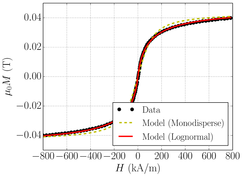
(a)

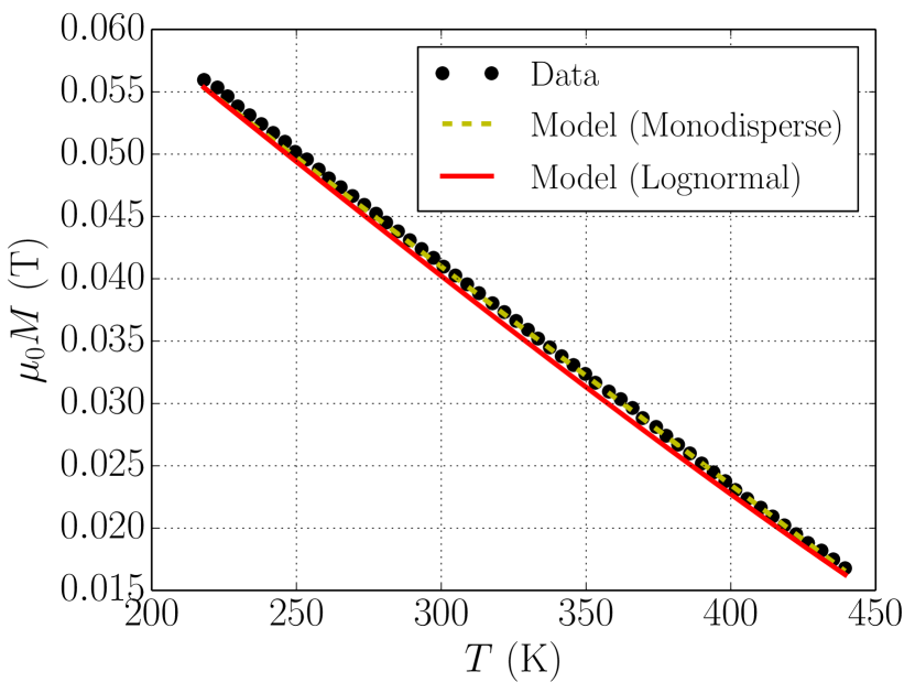
(b)

Figure 1: Fitting of models to magnetization data with (a) varying $H$ at constant $T=$300.1\text{\,}\mathrm{K}\text{/}$$, and (b) varying $T$ at constant $H=$796.0\text{\,}\mathrm{kA}\text{/}\mathrm{m}$$.

These models may then also be used to describe the magnetization response in TS50K with hexane, since the particles are the same. The total magnetization will be lower though, since $\alpha_{\mathrm{p}}$ is lower. The parameters of the best fit are shown in Tab. 4, and the corresponding size distribution is shown in Fig. 2.

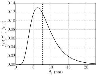
Figure 2: The log-normal diameter distribution fitted to magnetization data, with the median shown as a dashed line. The distribution represents how the total volume of particles is distributed across different diameters.

4.1.3 Model ferrofluid parameters

A summary of all the adjustable parameters in the model used in this work is shown in Tab. 4. The equation of state for the base fluid involves additional parameters, but they are not listed here, as they are not specific for this model or case, but part of a generalized thermodynamic library.

Table 4: Summary of parameters defining the ferrofluid in this model. Parameters marked with N/A are relevant for the model in general, but not in the specific validation cases in this work.

[b] Description Value Ferroliquid Viscosity $\eta_{\mathrm{f}}$ $2.35\text{\times}{10}^{-3}\text{\,}\mathrm{Pa}\text{\,}\mathrm{s}\text{/}$ Thermal cond. $\lambda_{\mathrm{f}}$ $0.16\text{\,}\mathrm{W}\text{/}\text{(}\mathrm{m}\text{\,}\mathrm{K}\text{)}$ Base fluid Vapor viscosity $\eta_{\mathrm{v}}$ $7.98\text{\times}{10}^{-6}\text{\,}\mathrm{Pa}\text{\,}\mathrm{s}\text{/}$ Vapor thermal cond. $\lambda_{\mathrm{v}}$ $0.0188\text{\,}\mathrm{W}\text{/}\text{(}\mathrm{m}\text{\,}\mathrm{K}\text{)}$ Components C11H24, C6H14 Mass composition 65%/35% Hexane surf. tens. $\sigma_{1}$ $1.17\text{\times}{10}^{-2}\text{\,}\mathrm{N}\text{/}\mathrm{m}$ Undecane surf. tens.¹ $\sigma_{2}$ $1.88\text{\times}{10}^{-2}\text{\,}\mathrm{N}\text{/}\mathrm{m}$ Particles Density $\rho_{\mathrm{p}}$ $5323\text{\,}\mathrm{kg}\text{/}{\mathrm{m}}^{3}$ Spec. heat cap. $c^{p}_{\mathrm{p}}$ $704.5\text{\,}\mathrm{J}\text{/}\text{(}\mathrm{kg}\text{\,}\mathrm{K}\text{)}$ Thermal cond. $\lambda_{\mathrm{p}}$ (N/A) Inlet volume fraction $\alpha_{\mathrm{p}}^{\circ}$ 0.0914 Mean diameter $d_{\mathrm{p}}^{\text{med}}$ $7.58\text{\,}\mathrm{nm}\text{/}$ Diameter std.dev. $d_{\mathrm{p}}^{\text{std}}$ $3.96\text{\,}\mathrm{nm}\text{/}$ Sat. mag. at $T^{\circ}$ $M^{\circ}_{\text{sat}}$ $265\text{\,}\mathrm{kA}\text{/}\mathrm{m}$ Curie temperature $T_{\text{C}}$ $576\text{\,}\mathrm{K}\text{/}$

• Average of values for decane and dodecane

4.2 The experimental rig

The experimental rig of Iwamoto et al. [11] consisted of a thermomagnetic pump (solenoid and heater) wrapped around a $1\text{\,}\mathrm{cm}\text{/}$ pipe, all of which could be tilted. In each case, the pressure difference across specified inlet and outlet points around the thermomagnetic pump was measured. A control system elsewhere in the loop kept the inlet conditions at approximately $p_{\mathrm{in}}=$1.163\text{\,}\mathrm{bar}\text{/}$$, $T_{\mathrm{in}}=$307\text{\,}\mathrm{K}\text{/}$$ and $v_{\mathrm{in}}=$2.0\text{\,}\mathrm{cm}\text{/}\mathrm{s}$$. The exact geometry of the setup is shown in Fig. 3, drawn from [11] and additional information supplied by its authors [33].

The geometry of the solenoid is shown to scale. It consists of about 850 turns of copper wire. With the given geometry, fitting these turns requires a wire diameter of about $3.4\text{\,}\mathrm{mm}\text{/}$, giving a solenoid resistance of about $1\text{\,}\mathrm{\SIUnitSymbolOhm}\text{/}$. Obtaining $H_{\mathrm{max}}=$100\text{\,}\mathrm{kA}\text{/}\mathrm{m}$$ with this solenoid requires a current of $25\text{\,}\mathrm{A}\text{/}$, giving a voltage-drop of $25\text{\,}\mathrm{V}\text{/}$ and thus a power dissipation of about $600\text{\,}\mathrm{W}\text{/}$.

The heater is modelled as a constant pipe wall temperature, while the pipe is approximated as perfectly insulated elsewhere. The heater temperature is specified in relation to $T_{\mathrm{in}}$, as a difference $\Delta T$.

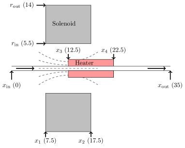
Figure 3: A cross section of the experimental rig in [11], to scale in both the axial and the radial direction. The rig geometry is rotationally symmetric around the pipe axis. With the origin at the left and center of the pipe, numbers show positions in $\mathrm{cm}\text{/}$, with vertical and horizontal arrows giving axial and radial positions, respectively. Dashed lines illustrate the magnetic field lines giving magnetic pumping force. The direction of gravity with respect to this figure varies with the tilt of the rig. In the horizonal configuration, gravity points perpendicular to the flow direction. In the vertical configuration, gravity points opposite to the flow direction.

4.3 Heat transfer coefficient

An important model parameter is the heat transfer coefficient (HTC), which is needed when calculating the wall heat transfer term described in Sec. 2.3.4. This may either be set constant, or represented by one of many available correlations.

For the cases with $\Delta T=$70\text{\,}\mathrm{K}\text{/}$$, the heater wall temperature is above the bubble temperature of the fluid, and boiling heat transfer occurs. This is either subcooled or saturated boiling, depending on whether the local average fluid temperature is below or above the bubble temperature. Boiling heat transfer correlations have mostly been made for either saturated or subcooled boiling. A single validation case presented here may include both regimes, as the temperature rises along the pipe. For this reason, it is preferable to use correlations which extend to both regimes.

In this work, we attempt to use two different correlations where boiling occurs: Gungor and Winterton [34], which claims to give reasonable results in both regimes, and Chen [35], which was originally developed for saturated boiling, but is recommended for use in subcooled boiling in [36]. The equations do not explicitly account for the presence of nanoparticles in the liquid, but when used here we supply the ferroliquid transport properties in place of liquid transport properties. This should be sufficiently accurate under the assumption that the effects of boiling on heat transfer dominate over the effects of the nanoparticles.

4.4 Results

Simulations were run with the ferrofluid parameters shown in Sec. 4.1 and the rig set-up shown in Sec. 4.2. Here the focus is the effect of the magnetic field strength on the pressure jump from the inlet to the outlet, $\Delta p$, which represents the thermomagnetic pumping effect. The quantity $\Delta p$ is thus zero at zero field in each case, by definition. The quantity is plotted against $H_{\mathrm{max}}$, which is the maximum field in the solenoid.

For the case of $\Delta T=$70\text{\,}\mathrm{K}\text{/}$$, data sets are available in [11] for both the horizontal and vertical orientation. Here boiling heat transfer occurs, and simulations were run with the two boiling HTC correlations in Sec. 4.3. To demonstrate the sensitivity of the predictions to this, bands of prediction given a 25% uncertainty in the HTC are also shown. This is a common uncertainty estimate, but the actual uncertainty can be much larger in certain parameter areas [34]. For two values of $H_{\mathrm{max}}$, the outlet temperatures are available. In these cases, one may also adjust a constant HTC to achieve the correct outlet temperature in the model. Here the HTC in the reference zero-field point is assumed equal to the HTC in the point of lowest field. All these results are plotted together with the experimental data from [11] in Fig. 4 and 5 for the horizontal and vertical case, respectively.

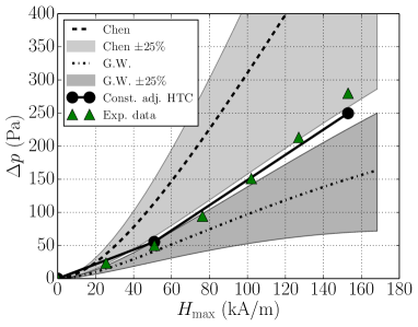
Figure 4: Results for the horizontal case with $\Delta T=$70\text{\,}\mathrm{K}\text{/}$$, compared with experiments from [11].

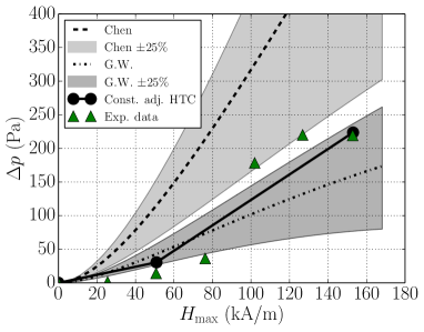
Figure 5: Results for the vertical case with $\Delta T=$70\text{\,}\mathrm{K}\text{/}$$, compared with experiments from [11].

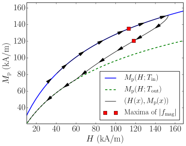
Figure 6: The particle magnetization curves at the inlet and outlet temperatures, and the path taken along the pipe, for a case with $\Delta T=$70\text{\,}\mathrm{K}\text{/}$$ and $H_{\mathrm{max}}=$153\text{\,}\mathrm{kA}\text{/}\mathrm{m}$$.

In the horizontal case, HTCs in the region $9001100\text{\,}\mathrm{W}\text{/}\text{(}{\mathrm{m}}^{2}\text{\,}\mathrm{K}\text{)}$ were needed to reach the measured outlet temperatures of approximately $352\text{\,}\mathrm{K}\text{/}$. In the vertical case, HTCs in the region $500900\text{\,}\mathrm{W}\text{/}\text{(}{\mathrm{m}}^{2}\text{\,}\mathrm{K}\text{)}$ were needed to reach the measured outlet temperatures of $338\text{\,}\mathrm{K}\text{/}$ and $348\text{\,}\mathrm{K}\text{/}$. In both cases, the Chen correlation predicted HTCs in the region $11002600\text{\,}\mathrm{W}\text{/}\text{(}{\mathrm{m}}^{2}\text{\,}\mathrm{K}\text{)}$, and reached temperatures of approximately $364\text{\,}\mathrm{K}\text{/}$, which is inside the liquid–vapor region. The Gungor–Winterton correlation predicted HTCs in the region $5001300\text{\,}\mathrm{W}\text{/}\text{(}{\mathrm{m}}^{2}\text{\,}\mathrm{K}\text{)}$, and reached temperatures of approximately $348\text{\,}\mathrm{K}\text{/}$.

Fig. 6 and 7 illustrate how the magnetization of the fluid changes through the rig, and how this leads to a net force. Fig. 6 shows the particle magnetization curves at the inlet and outlet temperatures, together with the $(M,H)$ path taken along the pipe. Fig. 7 shows the total magnetization as a function of pipe position $x$, together with $p$, $H$ and $T$. To the left of the solenoid center ($x<$0.125\text{\,}\mathrm{m}\text{/}$$), the field gradient $\frac{\partial{H}}{\partial{x}}$ and magnetization $M$ are positive, which leads to a positive magnetic force $f^{\text{mag}}=\mu_{0}M\frac{\partial{H}}{\partial{x}}$. Through the heating element ($$0.125\text{\,}\mathrm{m}\text{/}$<x<$0.225\text{\,}\mathrm{m}\text{/}$$) the temperature increases, which reduces the fluid magnetization. On the right side of the solenoid center ($x>$0.125\text{\,}\mathrm{m}\text{/}$$) the field gradient is negative, but due to the reduced magnetization, the negative force is less than the positive force on the left side. This then leads to a net positive pressure difference $\Delta p$.

Figure 7: Pressure, fluid magnetization, magnetic field and temperature as functions of distance $x$, for a case with $\Delta T=$70\text{\,}\mathrm{K}\text{/}$$ and $H_{\mathrm{max}}=$153\text{\,}\mathrm{kA}\text{/}\mathrm{m}$$.

5 Discussion

Without a symmetry-breaking temperature gradient, the solenoid only provides equal forces on each of its sides, pointing inwards. This would only lead to an internal pressure increase (and slight compression), and no net pressure increase from one side to the other. When combining Eqs. 14 and 31, one sees that the local magnetic force is essentially the product of $M_{\mathrm{p}}$, $\alpha_{\mathrm{p}}$, and $\mathop{\mathrm{\mathstrut d}}\nolimits\!H/\mathop{\mathrm{\mathstrut d}}\nolimits\!x$. To achieve net pumping action, the magnitude of this force must be decreased on one side of the solenoid compared to the other. There are two main mechanisms for achieving this:

First, the temperature sensitive particle magnetization leads to a decrease of $M_{\mathrm{p}}$ as the temperature increases. Second, a temperature increase leads to a decrease in the total density due to thermal expansion of the base fluid. Due to conservation of mass in steady state, i.e. constant $\rho v$, the velocity then increases during heating. According to Eq. 7, this must lead to a decrease in $\alpha_{\mathrm{p}}$ ($\rho_{\mathrm{p}}$ is constant), as the particle distribution is stretched thinner by the velocity increase. This effect can be very pronounced if there is a change from a liquid to a liquid–vapor state across the solenoid.

Both the above mechanisms are dependent on temperature, and thus the amount of heat transferred into the fluid from the pipe walls. As in any one-dimensional flow model, for a given temperature difference, this depends on the HTC (see Eq. 19).

This dependence was made clear in the attempt to validate against experimental data. From Fig. 4 and 5, it appears that the model is able to successfully predict the performance of the thermomagnetic pump, but only accurately if the prediction of temperature increase is good. As seen, in the simulations with a constant HTC adjusted to reach the correct outlet temperature, the predictions for $\Delta p$ are quite close to the measured ones. They are not in perfect agreement, but that may come from the fact that the whole temperature profile across the solenoid is important, not just the outlet temperature. The temperature at the right end of the solenoid is especially crucial, and as seen in Fig. 3, this is only halfway across the heater. The actual temperature profile is not likely to be equal to the one stemming from a constant HTC, even though they share the same outlet temperature.

In a usage scenario for e.g. application design and optimization, the temperature profile across the solenoid is most likely unknown, and must be predicted through using a correlation for the heat transfer coefficient. As we see from Fig. 4 and 5, the two correlations tested here both give $\Delta p$ in the correct order of magnitude, but differ considerably from both each other and the data. The results also show the very large sensitivity of $\Delta p$ to uncertainty in the HTC.

As we see from the gray bands, a $\pm 25\%$ uncertainty in the HTC will lead to an uncertainty of approximately $\pm 50\%$ in $\Delta p$. Combined with the fact that such correlations may have much higher uncertainties in some areas, especially when extrapolating from the data it is based on, it is apparent that careful use of appropriate HTC correlations is crucial when assessing the performance of a thermomagnetic pump.

In the validation cases used here, the heat transfer was of the boiling kind. It was assumed that this effect would dominate over any effects of nanoparticles, and thus conventional correlations for boiling heat transfer could be used. Since the predictions from using two different such correlations bracket the experimental data, it appears that this assumption was reasonable. However, for laminar flow without boiling, significant Nusselt number enhancements from the presence of nanoparticles are present [2, 3, 4], and correlations for these effects are not nearly as mature. High uncertainties must then be expected.

In vertical cases, it is worth noting that $\Delta p$ is the result of two competing effects: The positive contribution is the same as the one measured in horizontal cases. The new negative contribution from the magnetic field is due to the slight densification of the fluid caused by the pressure increase inside the solenoid (see Fig. 7). The magnetic field thus increases the hydrostatic pressure over the fluid column, decreasing $\Delta p$. Attempting to assist a natural convection loop with thermomagnetic pumping may thus have a detrimental effect if the solenoid is placed on a vertical section.

It is also worth noting that the design in Fig. 3 is not optimal for obtaining maximal $\Delta p$ from the given magnetic field. To achieve the largest symmetry breaking of the magnetic force, the temperature difference between the ends of the solenoid should be as large as possible. In terms of Fig. 6, the net pumping action achieved is loosely given by the area inside the loop. The vertical distance between the red squares is particularly important, as it shows the difference between the $M_{\mathrm{p}}$-factor in the peak rightward force and the peak leftward force. If the temperature were allowed to reach the outlet temperate before reaching the right end of the solenoid, the loop would be wider, and one would get more pumping action from the same solenoid and heat source.

The benefits of using a model of the kind presented here lie in its expected validity across a large range of parameters, which is very useful for process design and optimization. First of all, the flow equations (7)–(10) are generally applicable to any one-dimensional pipe configuration, no matter if the base fluid is single-phase or two-phase, as long as the no-slip assumption holds.

The crucial model for the ferroliquid magnetization, although complex, is physics-based and contains parameters which all carry physical meaning. The model retains the two critical features, S-shaped saturable response to external fields and reduction towards the Curie temperature, for any set of valid parameters. In contrast, a linearized model would have to fit new parameters each time the field or temperature changes considerably. Combined with the general equation for the solenoid field, this ensures a wide range of validity for the magnetic force term.

The thermodynamic model has the big advantage of being based on an equation of state for the base fluid, and thus takes advantage of the very large body of research on thermodynamic equations of state, which is not specific for nano/ferrofluids. This offers a big advantage over linearized or constant-property models, as one may perform design and optimization over a variety of pressure and temperature ranges with a number of base fluid components, without having to look up new model parameters. An equation of state enables the prediction of a large number of thermodynamic properties, given temperature and pressure, in an internally consistent way [12]. These properties, needed in the flow equations, as well as in various HTC correlations, include density (with compressibility and thermal expansion), heat capacity, enthalpy, latent heat of vaporization, critical pressure, bubble line, and liquid–vapor equilibrium. Implementations often include parameters for many possible components, and their interactions, so that one may change the base fluid components on-demand during usage. Equations of state are semi-empirical to various degrees, range from fast and simple to accurate and slow, and any of them may be used with this model.

A disadvantage is that equations of state are mainly fitted to equilibrium data, and thus can only reliably represent equilibrium states. The flow model can thus not account for the presence of vapor in subcooled boiling, besides by using an enhanced heat transfer coefficient, as is done in this work.

Overall, large flexibility and range of validity is expected from a model of the kind presented in this work. However, it is clear that there is a major sensitivity to uncertainties in the heat transfer coefficient, as would be the case for any one-dimensional heat transfer model with unknown temperature profiles. Other uncertainties and simplifying assumptions are obviously also present, but likely overshadowed by the above.

6 Conclusions and further work

We have presented a one-dimensional multi-phase flow model for simulating thermomagnetically pumped ferrofluid flow and heat transfer. The model includes a thermodynamic model which is a combination of a simplified particle model and thermodynamic equations of state for the base fluid. This enables a consistent treatment of partial vaporization of the base fluid, as could result from heat transfer to the ferrofluid. The model also includes a ferrofluid magnetization model, capable of taking into account effects of non-uniform particle size distributions. This magnetization model was shown to accurately reproduce experimental data on ferrofluid magnetization and its dependence on temperature and applied magnetic field. It was also shown that the presented multi-phase flow model was capable of predicting the thermomagnetic pumping mechanism, by which the temperature-dependence of the ferrofluid magnetization led to a net pumping pressure difference, and that the predicted pumping performance was in agreement with the experimental results from Iwamoto et al. [11].

It was, however, revealed that the predictions of thermomagnetic pumping are highly sensitive to the temperature profile in the pipe. Using good correlations for the heat transfer coefficient is therefore absolutely critical, and care must be taken to assure that a correlation is applicable to a given case. Due to this sensitivity, further research on the effects of nanoparticles on the heat transfer coefficient is called for.

Due to the generality of the models for thermodynamics and magnetization, the proposed model should have a large range of validity, given accurate heat transfer predictions. It could therefore be used for model-based optimization of designs for ferrofluid cooling devices over a wide range of parameters in further research.

Further validation of the model for additional cases would be beneficial, such as non-boiling heat transfer, and saturated liquid–vapor flow further inside the solenoid. However, this requires additional well-documented experiments.

References

References

- Choi and Eastman [1995] S. Choi, J. Eastman, Enhancing thermal conductivity of fluids with nanoparticles, URL http://www.osti.gov/scitech/servlets/purl/196525, 1995.
- Kakaç and Pramuanjaroenkij [2009] S. Kakaç, A. Pramuanjaroenkij, Review of convective heat transfer enhancement with nanofluids, International Journal of Heat and Mass Transfer 52 (13) (2009) 3187–3196, doi:10.1016/j.ijheatmasstransfer.2009.02.006.
- Xuan and Li [2000] Y. Xuan, Q. Li, Heat transfer enhancement of nanofluids, International Journal of Heat and Fluid Flow 21 (1) (2000) 58–64, doi:10.1016/S0142-727X(99)00067-3.
- Maiga et al. [2005] S. E. B. Maiga, S. J. Palm, C. T. Nguyen, G. Roy, N. Galanis, Heat transfer enhancement by using nanofluids in forced convection flows, International Journal of Heat and Fluid Flow 26 (4) (2005) 530–546, doi:10.1016/j.ijheatfluidflow.2005.02.004.
- Taylor et al. [2013] R. Taylor, S. Coulombe, T. Otanicar, P. Phelan, A. Gunawan, W. Lv, G. Rosengarten, R. Prasher, H. Tyagi, Small particles, big impacts: A review of the diverse applications of nanofluids, Journal of Applied Physics 113 (2013) 011301, doi:10.1063/1.4754271.
- Odenbach [2003] S. Odenbach, Ferrofluids—magnetically controlled suspensions, Colloids and Surfaces A: Physicochemical and Engineering Aspects 217 (2003) 171–178, doi:10.1016/S0927-7757(02)00573-3.
- Arulmurugan et al. [2006] R. Arulmurugan, G. Vaidyanathan, S. Sendhilnathan, B. Jeyadevan, Mn–Zn ferrite nanoparticles for ferrofluid preparation: Study on thermal–magnetic properties, Journal of magnetism and magnetic materials 298 (2) (2006) 83–94, doi:10.1016/j.jmmm.2005.03.002.
- Lian et al. [2009] W. Lian, Y. Xuan, Q. Li, Design method of automatic energy transport devices based on thermodynamic effect of magnetic fluids, International Journal of Heat and Mass Transfer 52 (2009) 5451–5458, doi:10.1016/j.ijheatmasstransfer.2009.06.031.
- Xuan and Lian [2011] Y. Xuan, W. Lian, Electronic cooling using an automatic energy transport device based on the thermomagnetic effect, Applied Thermal Engineering 31 (2011) 1487–1494, doi:10.1016/j.applthermaleng.2011.01.033.
- Lee et al. [2012] J. Lee, T. Nomura, E. M. Dede, Heat flow control in thermo-magnetic convective systems using engineered magnetic fields, Applied Physics Letters 101 (12) (2012) 123507–123507, doi:10.1063/1.4754119.
- Iwamoto et al. [2011] Y. Iwamoto, H. Yamaguchi, X.-D. Niu, Magnetically-driven heat transport device using a binary temperature-sensitive magnetic fluid, Journal of Magnetism and Magnetic Materials 323 (2011) 1378–1383, doi:10.1016/j.jmmm.2010.11.050.
- Michelsen and Mollerup [2007] M. L. Michelsen, J. M. Mollerup, Thermodynamic Models: Fundamentals & computational aspects, Tie-Line Publications, Holte, Denmark, second edn., ISBN 8798996134, 2007.
- Rosensweig [1985] R. E. Rosensweig, Ferrohydrodynamics, Cambridge University Press, Cambridge, ISBN 0486678342, 1985.
- Müller and Liu [2001] H. W. Müller, M. Liu, Structure of ferrofluid dynamics, Physical Review E 64 (2001) 061405, doi:10.1103/PhysRevE.64.061405.
- Tynjälä [2005] T. Tynjälä, Theoretical and Numerical Study of Thermomagnetic Convection in Magnetic Fluids, Ph.D. thesis, Lappeenranta University of Technology, 2005.
- Collier and Thome [1994] J. G. Collier, J. R. Thome, Convective boiling and condensation, Oxford University Press, Oxford, ISBN 0198562969, 1994.
- Lee and Kesler [1975] B. I. Lee, M. G. Kesler, A Generalized Thermodynamic Correlation Based on Three-Parameter Corresponding States, AIChE Journal 21 (3) (1975) 510–527, doi:10.1002/aic.690210313.
- Andersen [2010] J. O. Andersen, Introduction to Statistical Mechanics, The Norwegian University of Science and Techology, Department of Physics, Trondheim, ISBN 9788232101054, 2010.
- Chantrell et al. [1978] R. Chantrell, J. Popplewell, S. Charles, Measurements of particle size distribution parameters in ferrofluids, Magnetics, IEEE Transactions on 14 (5) (1978) 975–977, doi:10.1109/TMAG.1978.1059918.
- Maxwell [1873] J. C. Maxwell, A Treatise on Electricity and Magnetism, Clarendon press, Oxford, doi:10.1017/CBO9780511709333, 1873.
- Sobti and Wanchoo [2013] A. Sobti, R. K. Wanchoo, Thermal Conductivity of Nanofluids, Materials Science Forum 757 (2013) 111–137, doi:10.4028/www.scientific.net/MSF.757.111.
- Sundar et al. [2013] L. S. Sundar, K. V. Sharma, M. T. Naik, M. K. Singh, Empirical and theoretical correlations on viscosity of nanofluids: A review, Renewable and Sustainable Energy Reviews 25 (2013) 670–686, doi:10.1016/j.rser.2013.04.003.
- Brinkman [1952] H. Brinkman, The viscosity of concentrated suspensions and solutions, The Journal of Chemical Physics 20 (4) (1952) 571–571, doi:10.1063/1.1700493.
- Einstein [1906] A. Einstein, Eine neue Bestimmung der Moleküldimensionen, Annalen der Physik 324 (1906) 289–306, doi:10.1002/andp.19063240204.
- Jiles [1998] D. Jiles, Introduction to Magnetism and Magnetic Materials, Second Edition, Taylor & Francis, Boca Raton, ISBN 9780412798603, 1998.
- Meeker [2010] D. C. Meeker, Finite Element Method Magnetics, Version 4.2, URL http://www.femm.info, 2010.
- Jones et al. [01 ] E. Jones, T. Oliphant, P. Peterson, et al., SciPy: Open source scientific tools for Python, URL http://www.scipy.org/, 2001–.
- Hindmarsh [1983] A. C. Hindmarsh, ODEPACK, A Systematized Collection of ODE Solvers, IMACS transactions on scientific computation 1 (1983) 55–64.
- Piessens et al. [1983] R. Piessens, E. D. Doncker-Kapenga, C. W. Überhuber, QUADPACK: a subroutine package for automatic integration, Springer, Berlin, ISBN 3540125531, 1983.
- Iwamoto [2014] Y. Iwamoto, Personal communication (e-mail), additional information on TS50K, April 17. 2014.
- Eberhart [1966] J. G. Eberhart, The Surface Tension of Binary Liquid Mixtures, The Journal of Physical Chemistry 70 (4) (1966) 1183–1186, doi:10.1021/j100876a035.
- NIS [2014] NIST Chemistry WebBook, NIST Standard Reference Database Number 69, http://webbook.nist.gov, (retrieved November 4, 2014).
- Iwamoto [9 25] Y. Iwamoto, Personal communication (e-mail), solenoid schematics, 2014-09-25.
- Gungor and Winterton [1986] K. Gungor, R. Winterton, A general correlation for flow boiling in tubes and annuli, International Journal of Heat and Mass Transfer 29 (3) (1986) 351 – 358, doi:10.1016/0017-9310(86)90205-X.
- Chen [1966] J. C. Chen, Correlation for boiling heat transfer to saturated fluids in convective flow, Industrial & Engineering Chemistry Process Design and Development 5 (3) (1966) 322–329, doi:10.1021/i260019a023.
- Gungor and Winterton [1987] K. Gungor, R. Winterton, Simplified general correlation for saturated flow boiling and comparisons of correlations with data, Chemical engineering research & design 65 (2) (1987) 148–156.