Simultaneous VLBA polarimetric observations of the v=$\{$1,2$\}$ J=1-0 and v=1, J=2-1 SiO maser emission toward VY CMa II: component-level polarization analysis.

Abstract

This paper presents a component-level comparison of the polarized v=1 J =1-0, v=2 J=1-0 and v=1 J=2-1 SiO maser emission towards the supergiant star VY CMa at milliarcsecond-scale, as observed using the VLBA at $\lambda=7$mm and $\lambda=3$mm. An earlier paper considered overall maser morphology and constraints on SiO maser excitation and pumping derived from these data. The goal of the current paper is to use the measured polarization properties of individual co-spatial components detected across multiple transitions to provide constraints on several competing theories for the transport of polarized maser emission. This approach minimizes the significant effects of spatial blending. We present several diagnostic tests designed to distinguish key features of competing theoretical models for maser polarization. The number of coincident features is limited by sensitivity however, particularly in the v=1 J=2-1 transition at 86 GHz, and deeper observations are needed. Preliminary conclusions based on the current data provide some support for: i) spin-independent solutions for linear polarization; ii) the influence of geometry on the distribution of fractional linear polarization with intensity; and, iii) $\pi/2$ rotations in linear polarization position angle arising from transitions across the Van Vleck angle ($\sin^{2}{\theta}=2/3$) between the maser line-of-sight and magnetic field. There is weaker evidence for several enumerated non-Zeeman explanations for circular polarization. The expected 2:1 ratio in circular polarization between J=1-0 and J=2-1 predicted by standard Zeeman theory cannot unfortunately be tested conclusively due to insufficient coincident components.

1 Introduction

The nature and role of magnetic fields is an important open question in asymptotic giant branch (AGB), supergiant, and other late stages of stellar evolution. In late-type evolved stars, magnetic fields have been invoked to explain asymmetric mass loss (García-Segura et al., 2005), localised features such as arcs observed in the circumstellar material (Soker & Clayton, 1999; Soker, 2000), and the origin of circumstellar disks (Matt et al., 2000). Magnetic fields may also play a role in the presupernova collapse of massive stars (Heger et al., 2003).

The primary means to detect magnetic fields towards late-type evolved stars is through linear and circular polarisation observations of several distinct radiation emission mechanisms. Several factors favour longer-wavelength observations in such studies. These include: i) the high degree of visible obscuration for late-type evolved stars with high mass-loss rates; ii) the technical and sensitivity limitations of optical polarimetry for weakly-magnetic stars (Donati et al., 1997); and iii) the abundance of dust and molecular species in the circumstellar environment (CSE) of these objects with associated emission in the sub-millimeter or millimeter regime.

Magnetic fields have been detected towards planetary nebulae and protoplanetary nebulae by interferometric imaging of linearly-polarised continuum sub-millimetre emission, which traces dust alignment due to the magnetic field (Greaves, 2002; Sabin et al., 2007). The linear polarisation of molecular line emission can trace the magnetic field through the Goldreich-Kylafis effect (Goldreich & Kylafis, 1981), which has been observed in 620.701 GHz $5_{32}-4_{41}$ H₂O maser emission towards VY CMa (Harwit et al., 2010) and detected in thermal CO (J=2-1) and v=0, J-5-4 SiO emission toward IK Tau by Vlemmings et al. (2012). Optical spectropolarimetry has been used to detect magnetic fields of magnitude $\sim 100$ G in an active giant (Aurière et al., 2008), of order a few Gauss in several rapidly rotating giants (Konstantinova-Antova et al., 2009), $\sim 1$ G in the supergiant Betelgeuse (Aurière et al., 2010) and $\lesssim 1$ G in eight massive late-type supergiants (Grunhut et al., 2010). These detections used a least-squares deconvolution technique to find composite circular polarisation profiles from hundreds of observed optical spectral lines in order to mitigate sensitivity limitations noted above (Donati et al., 1997). The first detection of a photospheric magnetic field toward a Mira variable, the S-type star $\chi$Cyg, was recently reported using this technique by Lèbre et al. (2014), who measured a longitudinal magnetic field component of 2-3 G for this star. Sabin et al. (2015), using similar techniques, report longitudinal magnetic fields of 0.6 G and 10.2 G for the post-AGB stars R Scuti and U Monocerotis respectively.

Towards the end of a star’s lifetime, its mass loss increases and it can shed a considerable fraction of its mass through the stellar wind. This matter forms a dusty circumstellar envelope, which obscures the star at optical and infrared wavelengths (Iben & Renzini, 1983). Maser emission becomes a particularly important observational tool during these final stages of stellar evolution, as it is visible within dusty circumstellar envelopes (Cohen, 1989). OH, H₂O and SiO masers have all been used to measure magnetic fields in the circumstellar envelopes of late-type stars, where they sample the magnetic field over a range of distances from the star (Reid & Moran, 1981). OH maser observations of Zeeman patterns have been used to derive magnetic field estimates for evolved stars (e.g. Reid et al., 1979; Chapman & Cohen, 1986; Szymczak et al., 1998; Etoka & Diamond, 2004) and protoplanetary nebulae (e.g. Bains et al., 2003, 2004; Szymczak & Gérard, 2004; Gómez et al., 2009). Circular polarisation observations of H₂O masers have also been used to derive mangetic field estimates in the circumstellar envelopes of late-type evolved stars (e.g Vlemmings et al., 2002, 2005; Richards et al., 2004; Leal-Ferreira et al., 2013), in protoplanetary nebulae (Vlemmings & van Langevelde, 2008), and in the so-called water-fountain jet sources (Vlemmings et al., 2006). Similarly, circular polarisation studies of SiO masers have also been used to derive magnetic field estimates in the circumstellar envelopes of evolved stars (e.g. Barvainis et al., 1987; Kemball & Diamond, 1997; Amiri et al., 2012).

The high brightness temperature of maser emission makes it detectable at compact spatial scales with Very Long Baseline Interferometry (VLBI). SiO maser emission, in particular, can be imaged at milliarcsecond angular resolution in the inner circumstellar envelopes of late-type evolved stars (e.g. Diamond et al., 1994; Diamond & Kemball, 2003), making it a promising probe of the magnetic field at a distance of only a few stellar radii from the surfaces of these stars. However, in order for magnetic field information to be derived from the SiO maser polarisation observations, a maser polarisation radiative transfer model is required.

1.1 SiO maser polarisation theory

SiO is a non-paramagnetic molecule (Elitzur, 1992) and invariably falls into the weak-splitting Zeeman regime, where fully-separated Zeeman patterns are not observed (Gray, 2012).

The theory of polarized maser emission in this regime has been investigated in series of papers by Elitzur (e.g. Elitzur, 2002, and references therein), and by Watson and collaborators (e.g. Watson, 2002, and references therein). Both of these works build on the foundational maser polarisation theoretical model developed by Goldreich et al. (1973, hereafter GKK).

In the Elitzur model, circular polarisation of the maser emission is considered in the small-splitting regime primarily arising from the standard Zeeman effect, subject to the criteria that the maser polarisation has reached its stationary state and there is no significant magnetic field line curvature along the maser path (Elitzur, 2002); this model can be used to derive directly the magnetic field strength in the envelope from a measurement of circular polarization. In the Watson et al. models, multiple causes of circular polarisation are considered, including: i) the standard Zeeman effect alone; ii) the Zeeman effect with modifications due to saturation; and, iii) a change in quantisation axis as the maser propagates leading to the inter-conversion of linear to circular polarisation, termed non-Zeeman circular polarisation (Watson, 2002). The two bodies of theoretical work differ primarily in their foundational assumptions regarding the rate of establishment and stable propagation of stationary polarization modes; accordingly their predictions of maser polarization as a function of saturation frequently differ.

Gray (2003) compared the Elitzur and Watson models to the multi-level maser model by Gray & Field (1995). He found that the latter model level population equations could be reduced to those used by Watson (1994) thus anticipating similar model predictions. The theory of maser polarization is described in further detail in the monograph by Gray (2012). We note that Asensio Ramos et al. (2005) have considered the effect of radiation anisotropy and the Hanle effect on circumstellar SiO maser polarization. In addition, a recent paper by Houde (2014) considers anisotropic resonant scattering. In the current paper we focus primarily on testing current data against the core theories of Watson and Elitzur; future work will consider observational tests against more recent theoretical developments in the area of anisotropy in further detail.

Circumstellar SiO masers are strongly linearly polarised (e.g. Troland et al., 1979; Clark et al., 1982; Kemball & Diamond, 1997) and probably at least partially saturated (Nedoluha & Watson, 1994). In this parameter regime the observed circular polarisation could be created by either Zeeman or non-Zeeman effects. Furthermore, anisotropic pumping is a consideration for circumstellar SiO maser observations due to their proximity to the central star (Nedoluha & Watson, 1990a).

When observations of SiO maser circular polarisation are interpreted as due to the standard Zeeman effect alone, they imply circumstellar magnetic fields in the range of a few Gauss up to a few tens of Gauss in some cases (Barvainis et al., 1987; Kemball & Diamond, 1997). These magnetic field magnitudes imply a magnetic energy density of more than $\sim 10^{-0.5}$ dyne.cm^-2 (Reid, 2007). In contrast, the thermal pressure is $\sim 10^{-2.7}$dyne.cm^-2 and the ram pressure is $\sim 10^{-2.5}$dyne.cm^-2 in the SiO maser region of a typical AGB star circumstellar envelope (Reid, 2007). The magnetic energy density derived from the standard Zeeman interpretation is thus much greater than the thermal and ram energy densities. If this is the case, then the magnetic field may play a dominant role in the mass loss from the star and shaping of the envelope if globally organised (e.g. Matt et al., 2000; García-Segura et al., 2005). Alternatively, the SiO masers may be preferentially sampling strong localised magnetic fields with low global filling factors, caused by amplification of the tangential magnetic field due to shock compression around pulsating stars (Hartquist & Dyson, 1997; Kemball et al., 2009).

Under a non-Zeeman interpretation, the observed levels of circular polarisation could be created in the presence of magnetic fields of only a few tens of milliGauss (Nedoluha & Watson, 1994; Wiebe & Watson, 1998). For a magnetic field of this order the magnetic energy density is less than the thermal and kinetic energy densities in the SiO maser region. These uncertainties underline the scientific importance of placing closer observational constraints on the theoretical interpretation of SiO maser polarization data.

1.2 Overview

In this paper we systematically evaluate a number of observational tests designed to differentiate between the maser polarisation models discussed above, in order to improve the robustness of inferred magnetic field measurements from SiO maser emission observations. These tests entail component-level comparison of SiO maser features from the 43 GHz J=1-0 and 86 GHz J=2-1 transitions at milliarcsecond (mas) resolution, in order to minimize the effects of spatial blending. The supergiant star VY CMa was chosen as the target of this investigation, due to its high SiO maser luminosity over a wide range of SiO transitions (Cernicharo et al., 1993). The v=1 J=1-0, v=2 J=1-0 and v=1 J=1-0 SiO maser emission toward VY CMa was observed in full polarisation in this study, using the Very Long Baseline Array (VLBA^,). The first paper based on these data primarily addressed the overall maser morphology and implications for pumping and excitation (Richter et al., 2013, hereinafter Paper I). The current paper concerns a detailed component-level analysis of the data and resulting observational constraints on theories of maser polarization propagation. The current component-level analysis is confined to the epoch 2 data in Paper I, which have a significantly higher signal-to-noise ratio (SNR) than the earlier epoch 1 data.

The VLBA observations and their reduction are described in Section 2 and the results are presented in Section 3. Six observational tests of the polarisation models are proposed in Section 4, followed by their evaluation against the SiO data presented here. The conclusions are summarised in Section 5.

2 Observations and Data Reduction

Full-polarisation VLBA observations were performed on 15 and 19 March 2007, under project code BR123. The transitions ²⁸SiO v=$\{$0,1,2$\}$ J=1-0 and J=2-1, ²⁹SiO v=1 J=1-0 and ³⁰SiO v=0 J=1-0 were observed. We consider here only the ²⁸SiO v=$\{$1,2$\}$ J=1-0 and v=1 J=2-1 data, which were observed at adopted rest frequencies of 43122.03 GHz, 42820.48 GHz and 86243.37 GHz respectively (Müller et al., 2005). For each transition the spectral windows were centred in frequency assuming a systemic LSR (Local Standard of Rest) velocity of +18 km.s^-1 for the target source VY CMa.

These obsevations are described in detail in Paper I, which presents the total intensity and linear polarisation maps for each transition. The current paper presents the component-level linear and circular polarisation properties of the emission. A brief observational summary is provided below followed by a discussion of polarization calibration relevant to the current paper.

The target source VY CMa was observed in conjunction with continuum extragalactic sources 3C454.3, J0423-0120, J0609-1542 and 3C273, which were used as bandpass and continuum phase calibrators for all frequency bands. The data were sampled using two-bit quantisation, and correlated in full cross-polarisation over 128 frequency channels per spectral window. The 43 GHz lines were recorded in 8-MHz spectral windows and those in the 86 GHz band in 16-MHz spectral windows. The nominal velocity channel width in all spectral windows is therefore $\approx 0.43$ km.s^-1.

The data were reduced following methods outlined in Kemball & Richter (2011); these methods extend the calibration techniques described in Kemball et al. (1995) and Kemball & Diamond (1997) to allow high-accuracy Stokes $V$ measurement for millimeter-wavelength VLBI spectral-line observations. Data reduction refinements presented in Kemball & Richter (2011), and utilised here, include:

• Solving for and correcting the bandpass phase response offset between RCP (right circular polarisation) and LCP (left circular polarisation) receptors at the reference antenna.

• Applying an aliasing correction to the autocorrelation bandpass amplitude response, before re-use as part of the cross-correlation complex bandpass correction.

• The use of autocorrelation polarisation self-calibration; a coupled iterative solution for instrumental polarization and amplitude calibration using autocorrelation template spectral fitting.

• The use of a multi-antenna composite template spectrum during the latter amplitude calibration of the RCP and LCP receptor systems.

• The use of a global fit to continuum calibrator data to determine the differential R/L ampliude gain offset between the RCP and LCP receptor systems.

SiO	Clean beam	Nant	I peak	$\sigma_{I}$
transition	[$\mu$as]		[Jy/beam]	[Jy/beam]
v=1 J=1-0	$460\times 150$	10a	22.15	0.089
v=2 J=1-0	$430\times 140$	9b	12.16	0.134
v=1 J=2-1	$420\times 90$	8c	46.96	0.200

Table 1: Summary of the VLBA observations. For each SiO maser transition imaged, this table lists the major and minor angular dimensions of the CLEAN restoring beam, the number, N_ant, and configuration of VLBA antennas, the peak Stokes I brightness in the image cube, and the broadened thermal noise estimate $\sigma_{I}$ (as defined in Paper I).
^aVLBA antennas: BR, HN, KP, LA, MK, NL, OV, PT, SC, and a single VLA antenna; ^bVLBA antennas: BR, HN, KP, LA, MK, NL, OV, PT, SC; ^cVLBA antennas: BR, FD, KP, LA, MK, NL, OV, PT. (VLBA antenna abbreviations given in science.nrao.edu/facilities/vlba/docs/manuals/oss).

The data reduction was performed using a customised version of the Astronomical Image Processing System (AIPS). The observations are summarised in Table 1. For each SiO maser transition the table lists the CLEAN restoring beam major- and minor-axis angular dimensions, the antenna configuration, the peak Stokes I brightness (Jy/beam) in the resultant image cube, and the highest broadened thermal noise estimate $\sigma_{I}$ (Jy/beam) across all frequency channels of the imaged cube. The noise from all four Stokes parameters were broadened as described in Paper I, to account for un-modeled residual calibration and deconvolution errors in the off-source noise estimate. All of the resulting Stokes parameter errors presented in this paper are similarly broadened. The total time on the target source VY CMa was 150 minutes for each transition.

The linear polarisation absolute electric vector position angle (EVPA) was determined using ancillary Very Large Array (VLA). observations. The VLA observed the primary polarisation calibrator J0521+166 (3C138) and secondary polarisation calibrators J0646+448, J0609-1542, J0423-013 and J0542+498 in Q-band on 17 March 2007. At this time the array was in D configuration. The absolute EVPA of the primary polarisation calibrator 3C138 was adopted to be $-14^{\circ}$ (Perley & Taylor, 2003), and was used to calibrate the absolute EVPA of the secondary VLA polarisation calibrators. The secondary polarisation calibrators were then included in the VLBA observations to establish by reference the absolute EVPA of all remaining VLBA sources (equivalently, the residual unknown R-L phase difference at the reference antenna, assumed constant (Kemball, 1999)). It was not possible to use this method to perform absolute EVPA calibration of the 86 GHz data, as the VLA is not equipped to observe at this frequency.

2.1 Circular polarisation calibration

The VY CMa SiO maser emission is expected to be only weakly circularly polarised, at a level of a few percent (e.g. McIntosh et al., 1994; Herpin et al., 2006). Accurate calibration is therefore required for the circular polarisation measurements, as described in Kemball & Richter (2011).

As outlined in the previous section, the calibration method employed in this work solves for the differential R/L amplitude gains from a global fit to the continuum calibrator data. The calibrators J0423-1020 and J0609-1542 were used in this fit. No continuum circular polarisation has been detected towards J0423-1020 (Homan et al., 2001; Homan & Lister, 2006; Vitrishchak et al., 2008; Agudo et al., 2010). Continuum circular polarisation has been detected towards J0609-1542, at frequencies $\leq 8~{}$GHz (Homan et al., 2001; Homan & Wardle, 2003; Aller et al., 2003), and a $-0.23\%$ detection has been reported at 15 GHz (Homan & Wardle, 2003), as well as a more recent 15 GHz non-detection with an upper limit of $0.21\%$ (Homan & Lister, 2006). A non-detection with an upper limit of $0.53\%$ has been reported at 86 GHz (Agudo et al., 2010). Circular polarisation at a level of $\lesssim 0.5\%$ will not be significant relative to the noise in the work reported here, so J0609-1542 was also considered a suitable calibrator for the global continuum calibrator fit.

The errors $\sigma_{g_{0}^{RL}}$ in the R/L amplitude gains estimated using this method were determined using jackknife subsampling (Davison & Hinkley, 1997). Table 2 lists for each observed SiO transition, the reference differential R/L amplitude gain $g_{0}^{RL}$, associated jacknife error estimate $\sigma_{g_{0}^{RL}}$, and an independent measure of the error $\sigma_{m_{c}}$ in fractional circular polarization derived from continuum calibrator imaging of net residual Stokes $V$, described in further detail below.

SiO	Frequency	$g_{0}^{RL}$	$\sigma_{g_{0}^{RL}}$	$\sigma_{m_{c}}$
transition	band
v=1 J=2-1	86 GHz	0.990	$8.5\times 10^{-3}$	$0.61\%$
v=2 J=1-0	43 GHz	1.024	$7.5\times 10^{-3}$	$1.8\%$
v=1 J=1-0	43 GHz	0.993	$7.4\times 10^{-3}$	$0.00064\%$

Table 2: The circular polarisation accuracy parameters for the BR123 data sets. The columns from left to right are: the spectral line observed, the frequency band of the observation, the reference R/L amplitude gain $g_{0}^{RL}$, the jackknife error estimate $\sigma_{g_{0}^{RL}}$, and an independent measure of error $\sigma_{m_{c}}$ in fractional circular polarization, derived from continuum calibrator imaging tests.

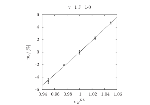
Figure 1: Plots of continuum calibrator circular polarisation, m_c, versus multiplicative R-L amplitude gain offset $\epsilon_{\mbox{g}^{RL}}$ for calibrator J0423-0120, for 43 GHz v=1 J=1-0 data (left), 43 GHz v=2 J=1-0 data (middle), and the 86 GHz v=1 J=2-1 data (right). For each data set a second-order polynomial was fitted to the data, which is plotted as a dashed line.

In this latter test, the accuracy of the spectral-line circular polarization amplitude calibration was independently assessed by applying the line amplitude calibration derived for the SiO maser source to a continuum calibrator source in the data set; the calibrator was then imaged after application of an additional, multiplicative $\epsilon_{\mbox{g}^{RL}}$ offset before allowing only residual phase calibration. This cross-calibration was repeated independently for a range of values $\epsilon^{RL}$, spanning unity. Further details of this test can be found in Kemball & Richter (2011). Calibrator J0423-1020 was chosen for this test because it is the brightest calibrator that was observed throughout the schedule.

Ten iterations of phase-only self-calibration were performed for each $\epsilon_{\mbox{g}^{RL}}$ data set constructed in this manner, imaging down to a final deconvolution threshold of a few times the thermal noise limit. The J0423-1020 data from the J=1-0 observation were imaged with pure uniform weighting. For the J0423-1020 data from the J=2-1 observation, Briggs weighting with a robustness parameter of zero (Briggs, 1995) was found to produce superior imaging performance. This calibration and imaging procedure for J0423-1020 was performed independently for multiplicative $\epsilon_{\mbox{g}^{RL}}$ offsets of 0.95, 0.975, 1.0, 1.025 and 1.05.

However, J0423-0120 was only observed for nine scans of approximately seven minutes each over the course of the observations, so the data set does not contain a large number of visibilities. Furthermore, the number of unflagged visibilities is further reduced after interpolating the VY CMa amplitude calibration gains onto J0423-0120, as there are time interval limits over which the line calibration solutions may reasonably be interpolated. A range of interpolation methods and flagging limits were investigated to determine the optimal interpolation parameters. These retain enough data to image while removing data where interpolation errors are most extreme. The optimal interpolation method was found to be a three-point median window filter with an interpolation limit of 14.25 minutes, half the length of a VY CMa scan.

The measured image-plane calibrator circular polarisation percentages for each $\epsilon_{\mbox{g}^{RL}}$ offset value are plotted in Figure 1. The circular polarisation was calculated from average Stokes I and V values, measured in a tight image box enclosing the central Stokes I emission. If the relative amplitude gains between the RCP and LCP data are correct, we would expect a m${}_{c}=0$ intercept for $\epsilon_{\mbox{g}^{RL}}=1$. The deviation of the m_c intercept from zero provides a conservative upper bound $\sigma_{m_{c}}$ on the error in the $R/L$ line amplitude calibration, given the inherent interpolation errors between line and continuum scans in this test. A second-order polynomial was fitted to each measured sequence $m_{c}(\epsilon_{g^{RL}})$; values computed at $m_{c}(\epsilon_{g^{RL}}=1)$ are listed in the right-most column of Table 2.

For the v=2 J=1-0 data set, the calibrator imaging test gives a particularly poor result, with an estimated $\sigma_{m_{c}}=1.8\%$ (Table 2; Figure 1). Of the three calibrator data sets, the imaging artifacts were most extreme for the Stokes $V$ v=2 J=1-0 data set J0423-1020 images, with deep off-source negatives around the central source region. If the Stokes $V$ values for this data set are averaged over a larger box incorporating the negative regions around the Stokes $I$ source position, then the fitted $\epsilon_{\mbox{g}^{RL}}=1$ intercept occurs at $\|$m${}_{c}\|\leq 0.5\%$. Thus, this independent estimate of error is at its limit of applicability for this transition, as discussed further below.

Outside of this discrepant v=2 J=1-0 calibrator imaging result, Table 2 shows that the errors in the R/L amplitude gain solutions are $\leq 1\%$. Kemball & Richter (2011) estimate the accuracy of the circular polarisation calibration method applied to VLBA observations of SiO maser emission towards TX Cam to be $\leq 0.5-1\%$ at 43 GHz and $\leq 1\%$ at 86 GHz. These ranges are consistent with the jacknife error estimates $\sigma_{g_{0}^{RL}}$ in Table 2. The poorer performance reported for the v=2 J=1-0 calibrator imaging test in the current work is due in part to the greater angular separation between the target source VY CMa and calibrators J0423-1020 and J0609-1542, compared to the angular separation between the source and calibrators used in Kemball & Richter (2011), as well as the low elevation of VY CMa. Both effects heighten interpolation errors in this test. The current data set also contained fewer calibrator observations than that used in Kemball & Richter (2011).

3 Results

For each transition, the peak intensity (over frequency channel) is plotted as a single-contour plot in Figure 2, colour-coded and overlaid by transition, at a contour level of 5$\sigma_{I}$. This follows Figure 8 in Paper I and defines features F1-F6, and includes a circle denoting the estimated stellar diameter (see Section 4 below). Absolute astrometric positions are lost during the data reduction process, due to the use of phase self-calibration (Thompson et al., 2004), so the relative alignment of the transition maps is unknown a priori. As described in Paper I the relative alignment was instead determined using a cross-correlation method and this alignment is used in Figure 2. The uncertainty in the map alignment is estimated to be $<0.05$ mas (Paper I). The maps of the v=2 J=1-0 and v=1 J=2-1 SiO maser transitions were restored with the same beam size as the v=1 J=1-0 SiO maser map, to allow component-level comparison of maser features.

Figure 2: Overlaid single-contour total intensity plots of the peak Stokes $I$ brightness over frequency for the SiO transitions v=1 J=1-0 (blue), v=2 J=1-0 (green), and v=1 J=2-1 (red). The contour level is $5\sigma_{I}$. The relative astrometric alignment was determined using a cross-correlation method, as described in the text. The features F1 to F6 defined here are discussed in the text and plotted in Figures 4 through 9. A circle of diameter 18.7 mas representing the estimated stellar diameter is plotted at the adopted stellar position (described further in Section 4.3).

3.1 Maser feature parameters

Component-level parameters of the individual features in the full Stokes I image cubes were extracted using the three-dimensional source detection software Duchamp (Whiting, 2012). The detection threshold used in Duchamp was set to five times the broadened noise $\sigma_{I}$ in the channel with the highest root mean square (RMS) noise (Table 1). The minimum channel width for feature detection was set to two channels, as the narrowest line widths of SiO maser features are typically $\sim 0.5$ km/s (Glenn et al., 2003).

The catalogue of maser features detected with Duchamp in Stokes $I$ is presented in Appendix A. The table lists the mean velocity $v$ and velocity extent $\Delta v$ of each feature. The Stokes $Q$, $U$ and $V$ brightness values for each feature were taken to be the associated value of the emission at the pixel position of maximum Stokes $I$ in the feature. The quoted errors $\{\sigma_{I}$, $\sigma_{Q}$, $\sigma_{U}$, $\sigma_{V}\}$ in the Stokes parameters use broadened off-source noise estimates, as described above.

The fractional circular polarisation m_c, fractional linear polarisation m_l, and the EVPA $\chi$ were derived from the measured Stokes $I$, $Q$, $U$ and $V$ brightness values. The uncertainties in m_c, m_l and $\chi$ are also included in the tables, calculated through propogation of the Stokes parameter errors.

The positions in the table are given as offsets ($\Delta\alpha$, $\Delta\delta$) on the projected plane of the sky, measured in milliarcseconds and increasing in the direction of increasing right ascension and declination. The offset is measured from the adopted centre of the map after relative alignment of the maser maps in each transition.

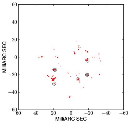
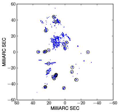
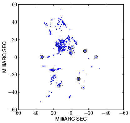
Figure 3: Linearly (left) and circularly (right) polarised features, from Tables A to LABEL:tab:BR123D1-components, for v=1 J=2-1 (red), v=1 J=1-0 (blue) and v=2 J=1-0 (green). The fractional polarisation of each feature is represented by a circle centered on the position of the feature, with the gray scale level of the circle increasing in proportion to the absolute fractional polarization of the feature. For the circularly-polarised features, the black border of the circle denotes whether $m_{c}>0$ (solid) or $m_{c}<0$ (dashed). The $|m_{c}|$ values fall in the range [$1.2\%$,$7.1\%$] and the $m_{l}$ values fall in the range [$1.6\%$,$46.5\%$].

Calculation of the measured linearly-polarized intensity $P$ are intrinsically biased due to the Ricean probability distribution of the non-negative $P=\sqrt{Q^{2}+U^{2}}$. This bias is taken into account by using the correction $P^{\prime}=\sqrt{P^{2}-\sigma_{QU}^{2}}$ (Wardle & Kronberg, 1974). The noise levels in the Stokes $Q$ and $U$ maps are similar, so the assumption is made that $\sigma_{Q}\sim\sigma_{U}$ in this analysis, and the geometric mean denoted as $\sigma_{QU}=\sqrt{\sigma_{Q}\sigma_{U}}$. The fractional linear polarisation values $m_{l}$ listed in the appendix have this correction taken into account. There is no bias correction needed for the position angle $\chi$ (Wardle & Kronberg, 1974).

The non-Gaussian probability density functions of $m_{l}$ and $m_{c}$ must also be taken into account when assessing statistical significance of a polarisation detection. In each case a detection limit was established by considering the null hypothesis that the fractional polarisation is equal to zero. The detection limit was set to the upper threshold of the $95\%$ probability interval for zero fractional polarisation. These values can be determined through numerical intergration of the probability density functions (PDF) for $m_{l}$ and $m_{c}$ (Kemball, 1992), but have well-behaved limit approximations.

The detection limit $u_{l}$ for the fractional linear polarisation can be approximated by a range estimator

$$u_{l}=\frac{1.65}{\sqrt{2}}\left[\frac{P^{\prime}+\sigma_{P^{\prime}}}{I-\sigma_{I}}-\frac{P^{\prime}-\sigma_{P^{\prime}}}{I+\sigma_{I}}\right]$$ (1)

where $\sigma_{P^{\prime}}=\frac{\sqrt{Q^{2}\sigma_{Q}^{2}+U^{2}\sigma_{U}^{2}}}{{P^{\prime}}}$ (Kemball, 1992). This prior work found that for m_l values up to $5\%$ the range estimator approximation $u_{l}$ is an underestimate of the detection limit by up to $10\%$. However, when the fractional linear polarisation is large the range estimator may overestimate $u_{l}$ by $35\%$. In the catalogues in Appendix A, only values of $m_{l}$ exceeding the detection limit $u_{l}$ are listed.

The $95\%$ probability interval for the fractional circular polarisation $m_{c}$ can be calculated using the Geary-Hinkley transformation, as described by Hayya et al. (1975), to yield upper and lower limits of

$$\mbox{u}_{c}=\pm 1.96\frac{\sigma_{V}}{\sqrt{\mu_{I}^{2}-1.96^{2}\sigma_{I}^{2}}}$$ (2)

This approximation is good to within $5\%$ when $\sigma_{I}<0.39\mu_{I}$ and $\sigma_{V}>0.005\mu_{V}$, where $\mu_{I}$ and $\mu_{V}$ are the mean values of Stokes parameters $I$ and $V$ (Hayya et al., 1975). These conditions are met for features listed in the Appendix catalogue. Only circular polarisations greater than the detection limit $u_{c}$ are listed in the Appendix.

The features which display statistically-significant linear and circular polarisation are shown in Figure 3.

3.2 Sub-feature level parameter extraction

Six maser features extended across angular position and frequency were chosen for more detailed polarisation analysis. The features were chosen based on their spatial coincidence, or near spatial coincidence, in multiple SiO maser transions and are labelled F1 to F6 in Figure 2.

The features and their spectra are plotted in Figures 4 through 9. Where the features consist of multiple distinct maser spots, separated in position or frequency, the spots are labelled separately in the figures and separate spectra are plotted for each.

In these Figures, contour plots of overlapping v=1 J=1-0 (blue), v=2 J=1-0 (green) and v=1 J=2-1 (red) Stokes $I$ emission are shown for each feature. The contours are drawn at levels $\{3\sigma_{I},5\sigma_{I}\}$, in terms of the broadened off-source noise limits described above. If contours for a particular transition are absent, the emission from that transition is weaker than the lowest contour. Associated EVPA plots overlaid on total intensity contour plots are also provided for those transitions with statistically-significant linear polarisation.

The accompanying Stokes $I$ spectra in these Figures were calculated from the peak Stokes $I$ pixel brightness values measured for each frequency channel across the feature. A threshold cutoff of three times the broadened noise in each channel was applied across the spectrum. The associated Stokes $Q$, $U$ and $V$ brightness values were measured at the pixel position of the Stokes $I$ maximum, and $m_{l}$ and $m_{c}$ computed accounting for statistical bias and the detection limits described above. For features where statistically-significant linear or circular polarisation was measured, the percentage polarisation values are shown in separate spectra.

In all spectra, the v=2 J=1-0 frequency axes are shifted by two channels ($\sim 0.86$ km s^-1) to account for an observed $\sim 2$ channel frequency offset between the positions of maser features in the v=2 J=1-0 transition, and the v=1 J=1-0 and v=1 J=2-1 transitions. As described in Paper I, the offset is likely due to errors in the assumed rest frequencies of these transitions.

Figure 4: Emission properties of feature F1, which is defined in Figure 2.
Left, top to bottom: i) Overlaid contour plot of the v=1 J=1-0 (blue), v=2 J=1-0 (green) and v=1 J=2-1 (red) maser emission drawn at contour levels of $\{3\sigma_{I},\ 5\sigma_{I}\}$; ii-iv) contour plots of the v=1 J=1-0, v=2 J=1-0 and v=1 J=2-1 emission at a total-intensity contour level of $\{3\sigma_{I}\}$, overlaid with vectors proportional in length to the underlying linearly polarized intensity on a scale where 1 mas = $27.78\times 10^{-3}$ Jy/beam. The vector orientation is in the direction of absolute EVPA for the J=1-0 lines (ii-iii; see text for J=2-1 EVPA alignment). The synthesised beam is drawn in lower-left of frames (ii) to (iv), and is $0.46\times 0.15$ mas in half-power at a position angle of $-1.80^{\circ}$.
Right, top to bottom: i) Feature spectra of Stokes $I$ intensity; ii) percentage linear polarisation, and iii) percentage circular polarisation over line-of-sight LSR velocity (in km/s). The upper axis of the Stokes $I$ spectrum shows the x-position at each velocity channel across the feature where the v=1 J=1-0 Stokes parameters were measured.

Figure 5: Emission properties of feature F2, which is defined in Figure 2.
Top, left to right: Overlaid contour plot of the v=1 J=1-0 (blue) and v=1 J=2-1 (red) maser emission, as for Figure 4; Contour plot of the v=1 J=1-0 emission overlaid with linear polarisation EVPA vectors, as for Figure 4. Bottom, left to right: Stokes $I$ spectrum of the feature and percentage linear polarisation spectrum of the feature, as for Figure 4.

Figure 6: Emission properties of feature F3, which is defined in Figure 2.
Top to bottom: Overlaid contour plot of the v=1 J=1-0 (blue), v=2 J=1-0 (green) and v=1 J=2-1 (red) maser emission, as for Figure 4; Contour plot of the v=1 J=1-0 emission overlaid with linear polarisation EVPA vectors, as for Figure 4. Stokes $I$ intensity and percentage linear polarisation spectra of the feature, as for Figure 4.

Figure 7: Emission properties of feature F4, which is defined in Figure 2.
Top to bottom: Overlaid contour plot of the v=1 J=1-0 (blue) and v=1 J=2-1 (red) maser emission, as for Figure 4; Contour plot of the v=1 J=1-0 emission overlaid with linear polarisation EVPA vectors, as for Figure 4. Contour plot of the v=1 J=2-1 emission overlaid with linear polarisation EVPA vectors, as for Figure 4, except that the vector length scale is 1 mas = $83.33\times 10^{-3}$ Jy/beam. Stokes $I$ intensity, percentage linear polarisation and percentage circular polarisation spectra for each of the spots in the feature, as for Figure 4.

Figure 8: Emission properties of feature F5, which is defined in Figure 2.
Top to bottom: Overlaid contour plot of the v=1 J=1-0 (blue) and v=1 J=2-1 (red) maser emission, as for Figure 4; Contour plot of the v=1 J=1-0 emission overlaid with linear polarisation EVPA vectors, as for Figure 4. Stokes $I$ intensity, percentage linear polarisation and percentage circular polarisation spectra for each of the spots in the feature, as for Figure 4.

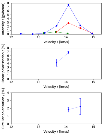
Figure 9: Emission proporties of feature F6, which is defined in Figure 2.
Top to bottom: Overlaid contour plot of the v=1 J=1-0 (blue), v=2 J=1-0 (green) and v=1 J=2-1 (red) maser emission, as for Figure 4; Contour plot of the v=1 J=1-0 emission overlaid with linear polarisation EVPA vectors, as for Figure 4. Stokes $I$ intensity, percentage linear polarisation and percentage circular polarisation spectra for each of the spots in the feature, as for Figure 4.

4 Discussion

The foundational analysis of maser polarisation was provided by Goldreich et al. (1973) (GKK), who treated the maser emission semi-classically, with the molecules modeled in a quantum mechanical framework, and the radiation field modeled in a classical framework. The GKK polarisation solutions were derived in several limiting cases, defined by the relative values of the stimulated emission rate $R$ (s^-1), the decay rate $\Gamma$ (s^-1), the Zeeman splitting $g\Omega$ (Hz) and the spectral width of the line $\Delta\omega$ (Hz). Astrophysical SiO masers are in the weak-splitting regime $\Delta\omega\gg g\Omega$ (Gray, 2012). As emphasized in a review by Watson (2002), the GKK solutions are an idealisation, as they deal with the specific case of a one-dimensional linear maser in a J=1-0 transition, weak continuum seed radiation, a constant magnetic field, $m$-isotropic pumping, a homogeneous environment, and derive the solutions at the line centre only. As further noted by Watson (2002), GKK solutions are not a continuous set of maser polarisation solutions over a range of maser intensities, or levels of saturation. It is noted that the GKK solutions in the extreme limit of strong saturation are obtained by setting the derivatives of the Stokes parameters with respect to intensity (effectively equivalent to distance) to zero and solving the resulting algebraic equations for fractional polarisation.

Subsequent work extended the GKK solutions to higher-order $J$ transitions and to intermediate relative values of $(R,\Gamma,g\Omega,\Delta\omega)$, such as partial saturation. Additional effects such as $m$-anisotropic pumping and non-Zeeman mechanisms for producing circular polarisation have also been considered. In this paper we primarily consider the work by Elitzur (Elitzur, 2002, and references therein) and by Watson and co-authors (Watson, 2002, and references therein). Elitzur has principally taken an analytic approach, finding stationary polarisation solutions. The work by Watson and collaborators makes use of numerical solutions of the polarised radiative transfer equations. A key foundational difference between the two approaches is that in the Watson approach the GKK solutions are considered applicable strictly under the asymptotic limits under which they were formulated (Nedoluha & Watson, 1993), as described above. In this view, the limiting solutions are not considered applicable to observational data (Watson, 2009). In the Elitzur approach, however, only stationary solutions are assumed to propagate, and the maser emission will rotate into the stationary solutions well before saturation (Elitzur, 1996, 2002).

Based on parameter estimates, circumstellar SiO maser emission most likely falls in the $g\Omega\gg R$ or $g\Omega>R$ regime with $R>\Gamma$ or $R\gg\Gamma$ (Kemball et al., 2009; Watson, 2009; Assaf et al., 2013); we consider this regime for the remainder of the paragraph. Here the GKK linear polarisation solutions have a position angle either parallel to or perpendicular to the projected magnetic field. The Elitzur model reproduces the GKK results in this regime (Elitzur, 1991).

Under the Watson model the linear polarisation solutions only asymptotically approach the GKK solution at high levels of saturation (Western & Watson, 1984; Watson & Wyld, 2001). For high saturation the form of the linear polarisation as a function of the angle $\Theta$ between the magnetic field and the line of site is similar to the GKK solution, without the sharp cutoff at the $\Theta\approx 35^{\circ}$ break angle (Watson & Wyld, 2001, GKK). In these solutions, if $g\Omega>R,\Gamma$ the EVPA will similarly be either parallel or perpendicular to the projected magnetic field (Watson, 2002).

In contrast, in the $g\Omega\simeq R$ regime, which is believed less likely based on parameter estimates, the linear polarisation position angle as a function of $\Theta$ will vary in form with intensity (Nedoluha & Watson, 1990b). At $g\Omega\sim R$ the fractional linear polarisation varies significantly with intensity (Nedoluha & Watson, 1990a).

Linear polarisation can also be created by $m$-anisotropic pumping of the masers, in the absence of a magnetic field in the medium (Bujarrabal & Nguyen-Q-Rieu, 1981; Western & Watson, 1983), or in conjunction with a magnetic field (Western & Watson, 1984; Nedoluha & Watson, 1990a).

The primary cause of circular polarisation explored by the Elitzur model is standard Zeeman splitting in the presence of a magnetic field (Elitzur, 1996). The Watson models consider circular polarisation caused by standard Zeeman splitting, with modifications due to saturation effects (Watson & Wyld, 2001), as well as non-Zeeman circular polarisation created by the the inter-conversion of linear to circular polarization in the intermediate intensity regime, due to intervening turbulent magnetic field directions or Faraday rotation (Nedoluha & Watson, 1990b, 1994; Wiebe & Watson, 1998).

4.1 Faraday rotation

Faraday rotation is a potential factor in any of the maser polarisation models, as Faraday rotation along the maser path may reduce the levels of integrated linear polarisation (GKK) and rotate the linear polarization EVPA (Wallin & Watson, 1997).

Faraday depolarisation becomes significant when the length of the region of plasma traversed by the radiation becomes close to the length scale $1.2\times 10^{17}(\lambda^{2}\;n\;B_{||})^{-1}$ (cm) corresponding to a Faraday rotation of $\pi$ radians, where $\lambda$ is the wavelength of the radiation (cm), $n$ is the electron density of the plasma (cm^-3) and $B_{||}$ is line of sight magnetic field (G) as derived using standard definitions of rotation measure (e.g. Draine, 2011). The electron density in the SiO maser region of VY CMa is unknown. Excess 8.4 GHz emission has been measured around VY CMa (Knapp et al., 1995) and VLA continuum observations at 15, 22 and 43 GHz have been modelled as a radio photosphere extending out to 1.5-2 R_⋆ (Lipscy et al., 2005). The extended atmospheres of late-type evolved stars are known to be complex in their layered structure, chemical composition, and kinematics (Wittkowski et al., 2011; Ireland et al., 2011), and similar complexity is likely in their ionization structure. An inner chromospheric ionized component is detected in the supergiant $\alpha$ Ori in UV spectroscopy, with a peak electron density n${}_{e}\sim 10^{8}$ cm^-3 close to the photosphere and a low filling-factor at larger radii (Harper & Brown, 2006). The larger and cooler radio photosphere is believed ionized predominantly by photo-ionized metals, and lies predominantly interior to the SiO maser region (Reid & Menten, 1997; Gustafsson & Höfner, 2004, p.g. 149-245). The SiO masers in VY CMa lie at an approximate mean radius of $\sim 2.5$ R_⋆. Number densities of order $\sim 10^{10}$ cm^-3 and a mean temperature $1.4\times 10^{3}$K are predicted at this radius by the AGB atmosphere models of Ireland et al. (2011). A corresponding electron density estimate of order $10^{3}$ cm⁻³ is obtained at the SiO maser radius (Assaf et al., 2013) using the ionization model of Reid & Menten (1997). This is consistent with an earlier independent estimate by Wallin & Watson (1997). A higher estimate of order n${}_{e}\sim 5\times 10^{5}$ cm^-3 is obtained from the semi-empirical model of Harper et al. (2001) for the radio photosphere of $\alpha$ Ori if computed at the radius of the SiO maser emission. Significant uncertainties remain, specifically the fine-scale ionization conditions and spatial structure in the extended atmosphere, the relative abundance fractions of atomic or molecular hydrogen (Glassgold & Huggins, 1983; Wong et al., 2016), and the neutral number density predictions of contemporary extended atmosphere models (Wong et al., 2016).

If we assume a line of sight magnetic field in the range 0.5-1 G, somewhat higher than the mean level observed in the H₂O maser region around AGB stars (Vlemmings, 2007), and an electron density of $10^{3}$ cm^-3, the Faraday depolarisation length scale is of order 2 R_⋆ at 43 GHz and 9 R_⋆ at 86 GHz, where R_∗ is the stellar radius of VY CMa. Infrared-optical interferometric measurements of R_∗ range from $9.88\times 10^{11}$m (Wittkowski et al., 2012) to $1.68\times 10^{12}$m, the latter value derived from a stellar diameter measurement of 18.7 mas (Monnier et al., 2004); both values of R_∗ assume a distance of 1.2 kpc (Zhang et al., 2012). We conservatively adopt the larger value of R_∗ in our order-of-magnitude estimates of depolarization length, but this choice does not affect our conclusion. At the adopted electron density n${}_{e}\sim 10^{3}$ cm^-3 Faraday depolarisation is not be a significant effect, even for the lower frequency 43 GHz J=1-0 masers. However we note that this does not hold if electron densities approach the higher estimates of n${}_{e}\sim 5\times 10^{5}$ cm^-3.

Several additional results support the conclusion of lower Faraday rotation. Wallin & Watson (1997) performed numerical calculations of Faraday rotation in the weak-splitting regime, which showed that Faraday rotation in circumstellar SiO masers is not a dominant effect. Assaf et al. (2013) estimate a Faraday rotation of $\sim 16^{\circ}$ for the J=1-0 SiO masers toward R Cas. Faraday depolarisation of the maser emission would also result in higher levels of linear polarisation at higher $J$ levels (Elitzur, 1991); this pattern has not been unambiguously detected in prior single-dish studies (Section 4.3, Test 1). Substantial Faraday depolarization would be accompanied by a significant rotation of the linear polarisation position angle, which is not observed in prior single-dish observations that suggest depolarization (McIntosh & Predmore, 1993). Furthermore, numerous VLBI observations of SiO masers show the linear polarisation direction to be ordered, (e.g. Kemball & Diamond, 1997; Cotton et al., 2006; Assaf et al., 2013), with position angles predominantly tangential to the star, arguing against a large degree of Faraday rotation along the maser path.

4.2 Observational tests

Six observational tests of the SiO maser polarisation models are discussed below, to be evaluated with the multi-transition SiO maser observations of VY CMa presented in this paper. Tests that compare maser characteristics between different transitions are ideally performed using measurements of individual overlapping maser features, to ensure that the physical conditions of the masing gas are as similar as possible.

The tests are evaluated against observational data in the subsequent section, Section 4.3. Several of the tests have been performed previously, using single dish and interferometric observations, and these prior results are discussed along with the application of the tests to the current observations.

• Comparison of linearly-polarized intensity in the v=1 J=1-0 and J=2-1 transitions.

  Under the Elitzur model, SiO maser transitions have spin-independent linear polarisation solutions (Elitzur, 1991). Under the Watson model the J=1-0 transition will have greater linearly-polarized intensity, if the transitions are under comparable levels of saturation and degree of m-anisotropic pumping (Western & Watson, 1984; Nedoluha & Watson, 1990a).
  

• Comparison of intensity and fractional linear polarisation.

  The relationship between fractional linear polarisation and saturation level differs between maser polarisation models, as described above, and observational evidence for the form of this relationship would provide a means to discriminate between the models.

  However, the saturation level depends on the unknown beaming angle as well as brightness, and the functional form of the beaming angle varies with saturation (Elitzur, 1992). In consequence, maser intensity is an imperfect proxy for the unknown saturation level. Nonetheless, with this important disclaimer, the relationship between linear polarisation and intensity is a potential diagnostic indicator of the relationship between linear polarisation and saturation.

  In the Elitzur model the polarisation solution is not dependent on the saturation level of the masers, as long as the maser emission has evolved into the stationary solution (Elitzur, 1991). In the Watson model the fractional linear polarisation level increases slowly with saturation, only asymptotically approaching the GKK solution (Western & Watson, 1984; Nedoluha & Watson, 1990a). For $g\Omega\gg R$, a correlation of fractional fractional linear polarisation with saturation level would therefore be evidence for this model.

  Near $g\Omega\simeq R$, which is believed less physically likely as discussed above, fractional linear polarisation may decrease with increasing maser saturation (Nedoluha & Watson, 1990a). In this regime, the addition of m-anisotropic pumping leads to a reduction of fractional linear polarisation at higher saturation levels for the v=1 J=2-1 line than for the v=1 J=1-0 line (Nedoluha & Watson, 1990a).
  

• Comparison of fractional linear polarisation with distance from the star.

  Circumstellar maser emission that is anisotropically pumped by stellar radiation will be strongest closest to the star (Western & Watson, 1983; Desmurs et al., 2000). The fractional linear polarisation created by anisotropic pumping is therefore expected to be strongest closest to the star, where the anisotropy parameter is largest (Kemball et al., 2009). However, this trend may also be influenced by shock compression of the magnetic field in the inner layers of the near-circumstellar envelope (Kemball et al., 2009).
  

• Electric vector position angle rotation.

  Circumstellar SiO masers often show 90^∘ EVPA rotations across a single maser feature (e.g. Kemball & Diamond, 1997). One natural explanation is a transition over the feature across the critical $55^{\circ}$ angle between the magnetic field and the line of sight in the regime $g\Omega>R,\Gamma$, where the direction of the EVPA is predicted to change from parallel to perpendicular to the projected magnetic field direction (GKK; Elitzur, 2002; Watson, 2002).

  Under the Watson model, EVPA rotation can also occur in the $g\Omega\simeq R$ regime, with degree of rotation dependent on saturation (Nedoluha & Watson, 1994). This EVPA rotation is at most $\sim 45^{\circ}$ over an order of magnitude in saturation level, except for very large magnetic fields ($100$G) directed almost perpendicular to the line of sight ($75^{\circ}$). It is therefore unlikely that abrupt $\sim 90^{\circ}$ changes in EVPA are caused by this mechanism.

  Linear polarisation EVPA rotation can also be explained by $m$-anisotropic radiative pumping, over a change in anisotropy conditions (Western & Watson, 1983; Asensio Ramos et al., 2005). A change in the dominant anisotropy direction from radial to tangential could result in a 90^∘ polarisation EVPA flip, but only if the magnetic field is not dynamically significant (Asensio Ramos et al., 2005). In the presence of a magnetic field of order 10-100 mG EVPA rotation of about 45^∘ can occur, however with considerable suppression of the masing effect (Asensio Ramos et al., 2005).

  GKK-style EVPA flips can be modeled in features that contain a linear polarization EVPA position angle transition of 90^∘ by modeling the fractional linear polarization and its dependence on the variation of the angle $\Theta$ between the magnetic field and the line of sight $m_{l}(\Theta)$, along the maser feature (Kemball et al., 2011). If the functional form of $m_{l}(\Theta)$ across a 90^∘ EVPA flip is well-described by the GKK model, this is more supportive of the Elitzur models, because under the Watson model the fractional linear polarisation solutions approach the asymptotic GKK solution only at very high levels of saturation (Western & Watson, 1984; Watson & Wyld, 2001).
  

• Comparison of circular polarisation in the v=1 J=1-0 and J=2-1 transitions.

  The ratio of standard Zeeman splitting in the presence of a magnetic field to the Doppler line width is proportional to the wavelength of the transition (Elitzur, 1996). Standard Zeeman circular polarisation for the J=1-0 transition at 43 GHz should therefore be double that of the J=2-1 transition at 86 GHz, all other effects being equal.

  The standard Zeeman circular polarisation can be increased by a factor of a few due to saturation under the Watson model (Watson & Wyld, 2001). Saturation has no effect on the predicted circular polarisation under the Elitzur model, so long as J/J${}_{s}\;>\frac{3}{4}$, where J is the maser intensity, and J_s the saturation intensity (Elitzur, 1996).

  Under the Watson model, non-Zeeman circular polarisation can be created by a change in direction of linear polarisation. This can occur when the maser emission falls in the $g\Omega\sim R$ regime, when the magnetic field direction changes along the line of sight, or when Faraday rotation is significant (Watson, 2009).

  These non-Zeeman circular polarization mechanisms do not depend strongly on the angular momentum level of the transition.
  

• Correlation between circular and linear polarisation.

  If the circular polarisation is caused by the non-Zeeman effects described in the previous sub-section, then the level of circular polarisation will be correlated with the level of linear polarisation (Watson, 2009). This correlation can be destroyed by statistical variations in the emission region, so the absence of this correlation is not necessarily evidence against non-Zeeman circular polarisation (Wiebe & Watson, 1998). However, if many maser features display circular polarisation at a level much greater than the average value of $m_{l}^{2}/4$, then the circular polarisation is unlikely to be caused by non-Zeeman effects (Wiebe & Watson, 1998).

4.3 Observational test evaluation

• Comparison of linear polarisation in the v=1 J=1-0 and J=2-1 transitions.

  Single-dish observations over a sample of sources by Barvainis & Predmore (1985) show strongly-correlated and comparable spectrum-averaged fractional linear polarisation $\overline{m_{l}}_{s}$ in the v=1, J=1-0 and v=2, J=2-1 transitions. Similarly, single-dish observations of these two transitions toward VY CMa (McIntosh et al., 1994) show broadly-comparable, or no clear trend, in values for fractional linear polarisation averaged in velocity over coincident spectral features $\overline{m_{l}}_{f}$. In contrast, a single-dish survey of late-type evolved stars in transitions v=1 J=1-0, v=1 J=2-1, and v=1, J=3-2 by McIntosh & Predmore (1991) is consistent with increasing $\overline{m_{l}}_{f}$ in higher rotational transitions. Similar measurements in these three transitions for features in the spectrum of Mira (McIntosh & Predmore, 1993) also generally favor a lower relative value $\overline{m_{l}}_{f}$ for the J=1-0 transition. Collectively, these prior results do not allow an unambiguous rank ordering.

  These previous observations were all performed with single dish telescopes, so spatial blending is a possible source of significant systematic error, as noted by the authors. Ideally, the linear polarisation should be compared at the component-level in features with spatially-coincident emission. In the current interferometric study, the only two features meeting these conditions that showed statistically significant linear polarisation in both v=1, J=1-0 and v=1, J=2-1 transitions are feature F1 (Figure 4) and feature F4 (Figure 7).

  In feature F1 the linear polarisation is considerably greater in the v=1 J=2-1 line, with an average percentage linear polarisation of $32\%$ over the feature. The corresponding average in the v=1 J=1-0 line is $6\%$.

  In feature F4, only spot S1 shows significant linear polarisation in the v=1 J=1-0 line. In this spot, the linear polarisation level is similar for both transitions. Significant linear polarisation is only measured in two frequency channels across the J=1-0 feature, and three channels across the J=2-1 line. In both cases the peak linear polarisation is 8$\%$, measured at the brightest pixel of spot S1 in the peak Stokes $I$ channel.

  For features F2, F3, F6 and the other F4 spots, linear polarisation is detected in the v=1 J=1-0 line, but not in the v=1 J=2-1 line, possibly due to lower SNR. This was investigated by assuming that the v=1 J=2-1 masers are linearly polarised at the level of the v=1 J=1-0 masers, and checking if the J=2-1 linear polarisation would lie above the detection limits defined in Section 3.1 (and vice versa). For F2, F5 and F4 S3, linear polarisation at the level of the v=1 J=1-0 feature would have been detected in the J=2-1 line at the sensitivity of the current study. However, in features F3 and F4 S4 it would not have been detected.

  Feature,	Ordinal relation in ml	$\overline{\mbox{m}}_{l}$	$\overline{\mbox{m}}_{l}$	Note
  spot		J=1-0	J=2-1
  F1	J=2-1 $>$ J=1-0	6.3$\%$	32.0$\%$
  F2	J=1-0 $>$ J=2-1	16.4$\%$		$\star$
  F3		5.1$\%$
  F4 S1	J=1-0 $\sim$ J=2-1	5.8$\%$	6.8$\%$
  F4 S3	J=2-1 $>$ J=1-0		8.4$\%$	$\star$
  F4 S4			4.9$\%$
  F5	J=1-0 $>$ J=2-1	8.7$\%$		$\star$
  F6		5.5$\%$

  Table 3: Fractional linear polarisation comparison between the v=1 J=1-0 line and v=1 J=2-1 line.

  ^⋆ In these cases, linear polarisation is only detected for the more linearly-polarised line. However, equal or greater fractional linear polarisation for the missing line would have been detected within the sensitivity of the current observations.

  A summary of the these linear polarisation results is given in Table 3. The average fractional linear polarisation values $\overline{\mbox{m}}_{l}$ shown are computed over all detected linear polarisation values in the line or feature, without any requirement for multi-transition detection. However, for features F1 and F4 S1 the values listed in the table are the averages over the channel range where linear polarisation is detected in both lines.

  The average linear polarisation across all features in the source with linear polarisation detections, as enumerated in Appendix A, is 13.7$\%$ and 7.7$\%$ for the 43 GHz v=1 J=1-0 and v=2 J=1-0 emission, and 15.0$\%$ for the 86 GHz v=1 J=2-1 emission.

  The results in Table 3 show that more cospatial components are needed than are detected in both rotational transitions before a firm conclusion can be drawn regarding the relative magnitude of $\overline{m}_{l}$. However on the basis of the net ordinal relation in Table 3, and secondarily the mean $\overline{m}_{l}$ over all features in Appendix A, the current results are more consistent with the conclusion of comparable fractional linear polarization for both rotational transitions.

  Although component-level comparisons allow a more precise test of the dependence of fractional linear polarisation on rotational transition than is possible in single-dish studies, even at VLBI resolution the physical conditions probed may not be exactly identical in both transitions. For example, the large fractional linear polarisation difference in feature F1 could be explained through a small positional offset between the maser emission from the J=1-0 and J=2-1 transitions, translating to a small difference in angle $\Theta$ between the magnetic field and the line of sight. Different $\Theta$ implies a different fractional linear polarisation between the two transitions in the GKK model for $g\Omega\gg R\gg\Gamma$, as plotted in Figure 10. The offset in F1 fractional linear polarisation between the v=1 J=1-0 emission (6.3$\%$ on average) and the v=1 J=2-1 emission (32.0$\%$ on average) can be accounted for by the gradient over the region $Q/I\simeq-0.05$ to $-0.3$ which corresponds to a change in angle $\Theta<10^{\circ}$. Alternatively, field line curvature along the path length of the maser emission may reduce the observed linear polarisation. If the path length of the J=2-1 maser is a limited fraction of the path length of the J=1-0 maser, the effect of field line curvature will be diminished for the J=2-1 maser, possibly explaining the higher J=2-1 polarisation.

  Faraday depolarization predicts lower fractional linear polarization in J=1-0 accompanied by a large linear polarization position angle rotation between the two transitions; this EVPA rotation is not generally observed in the current data (Section 4.3, Test 4).
  

  

  Figure 10: Plot of the GKK fractional linear polarisation solution. Vertical lines are plotted through $Q/I=-0.32$ and $-0.063$ (see text for discussion).

• Comparison of saturation and linear polarisation.

  In Figure 11 the fractional linear polarisation is plotted against the total intensity for each of the maser features with statistically significant linear polarisation, separately for each transition. The plots show a general trend of higher linear polarisation for the weaker maser emission, particularly for the v=1 J=1-0 emission, for which the largest number of maser features were detected.

  

  Figure 11: Plots of fractional linear polarisation versus total intensity, for the v=1 J=2-1 (left), v=1 J=1-0 (centre), and v=2 J=1-0 (right) maser features.

  Trends of higher fractional linear polarisation for weaker SiO masers have previously been observed in the late-type evolved stars R Aquarii (Allen et al., 1989; Hall et al., 1990; Boboltz, 1997), R Cassiopeia (McIntosh et al., 1989; Assaf et al., 2013) and R Leo (Clark et al., 1984).

  A trend of decreasing fractional linear polarisation with saturation is at odds with the predictions of both Watson and Elitzur models in the regime $g\Omega\gg R\gg\Gamma$. However, in addition to the caveat noted above regarding the use of intensity as a proxy for saturation, there are very likely to be additional variables in play. We note that the observed trend of higher linear polarisation for the weaker masers has been previously hypothesized to result from relative saturation and m-anisotropic pumping near the regime $g\Omega\simeq R$ (Nedoluha & Watson, 1990a). As discussed above, this regime is believed less likely to be applicable to circumstellar SiO masers based on current parameter estimates. We also note that McIntosh et al. (1989) argue that stronger maser emission arises out of longer maser path lengths, these components may suffer the greatest levels of Faraday depolarisation leading to the observed trend in $m_{l}(I)$. However, for reasons discussed in earlier sections, there is no strong evidence of dominant Faraday depolarization effects in the SiO maser region.

  

  Figure 12: Plot of fractional linear polarisation versus total intensity, for the v=1 J=1-0 maser features. The colour scale is line-of-sight velocity in the LSR frame, in km/s, as shown in the color bar on the right. The adopted systemic LSR velocity for VY CMa is +18 km s^-1.

  Assaf et al. (2013) report higher fractional linear polarization in the inner shell of R Cas; by projection arguments the authors note that inner-shell features are more likely to be at extreme velocities in the spectrum. In Figure 12 we plot the linear polarization percentage against total intensity for all detected v=1, J=1-0 maser features, colour-coded by LSR velocity. As noted earlier, a systemic stellar velocity $V_{*}=+18$ km s^-1 has been adopted for VY CMa in the current work. Figure 12 shows a tendency of weak-$I$ high-m_l features to fall further from the stellar velocity and vice versa for high-$I$ weak-m_l features. Note that the highest $I$ feature on the figure, with m${}_{l}~{}6\%$, is the unusual feature F1.

  In the model of tangential amplification for circumstellar SiO masers (e.g. Diamond et al., 1994) longer coherent path lengths and higher intensities occur closer to the systemic stellar velocity $V_{*}$; to first order, maser features near this velocity are expected to lie closer to the plane of the sky. If the magnetic field structure is such that masers at velocities $V$ further from the systemic velocity are more likely to have smaller angles $\theta$ between the magnetic field and line-of-sight then under the GKK model for $m_{l}(\theta)$ for $g\Omega\gg R\gg\Gamma$ (Figure 10), or related functional forms for lower saturation in the models of Watson & Wyld (2001), a possible explanation is provided for the trends in $m_{l}(I)$ and $m_{l}(|V-V_{*}|)$ in Figure 12. This $\theta(V)$ dependence arises naturally with a radial magnetic field (Assaf et al., 2013), but may also arise from other local or global morphologies. These effects may also be enhanced by lower gradients in magnetic field along the maser path for smaller $|V-V_{*}|$.
  

• Comparison of linear polarisation with distance from the star.

  Time-series VLBA images of polarised SiO maser emission towards TX Cam and R Cas show strongest linearly-polarised intensity (Kemball et al., 2009) and fractional linear polarisation (Assaf et al., 2013) respectively at the inner boundary of the projected maser shell.

  Figure 13 shows the component-level fractional linear polarisation plotted against projected distance from the assumed stellar position, for the three transitions observed in the current paper. The stellar position is unknown, but we adopt the zeroth-order assumption that the central star is most likely located toward the centroid of the inner shell of SiO maser features. The position was estimated through a grid search of the inner 30 mas of the image, to find the the position which maximises the minimum projected distance of the candidate centroid position to the closest maser feature. The feature positions in Appendix A were used in this minimisation. A circle representing the star is shown on Figure 2, centred on the stellar position estimated using this method, and adopting a diameter of 18.7 mas from Monnier et al. (2004).

  

  Figure 13: Percentage linear polarisation versus projected radial distance from the assumed stellar position, for the v=1 J=1-0, v=2 J=1-0 and v=1 J=2-1 maser features.

  Zhang et al. (2012) determined the VY CMa stellar position relative to VLBA observations of the SiO masers through VLA observations of the radio photosphere. The stellar position assumed in this paper is coincident with the Zhang et al. (2012) position within the 10 mas uncertainty cited by these authors.

  There is no visible trend in Figure 13 of higher fractional linear polarisation closer to the star. However, we stress that VY CMa is a supergiant, with a complex circumstellar environment and likely asymmetric mass loss (described in greater detail in Paper I), so the absence of this correlation does not exclude anisotropic pumping.
  

• Electric vector position angle rotation.

  Analysis of individual SiO maser features with 90^∘ EVPA rotations were performed by Kemball et al. (2011) and Assaf et al. (2013) who found that the EVPA rotation and percentage linear polarisation were consistent with the GKK linear polarisation solution for $g\Omega\gg R\gg\Gamma$. This solution for $m_{l}(\theta)$ is shown in Figure 10, where $\theta$ is the angle between the magnetic field and the line-of-sight.

  In the current data, features F1 and F2 are candidates for a similar analysis.
  

  Feature F2

  Following Kemball et al. (2011), a fit was performed for the fractional linear polarisation in v=1, J=1-0 across feature F2 (Figure 5), modeling the angle $\Theta$ as a second order polynomial in projected angular distance along the feature,

  $$\Theta=p\;(d-d_{55})^{2}+q\;(d-d_{55})+55$$ (3)

  where $\Theta$ is in units of degrees and $d_{55}$ is the projected angular position of the minimum in the polarised emission, at the mid-point of the $90^{\circ}$ EVPA rotation. The projected angular distances were measured radially from the assumed stellar position. The measured fractional linear polarisation values were jointly fit to Equation 3 and the GKK linear polarisation solution described earlier in this section, using a $\chi^{2}$-fit for parameters $p$ and $q$. The results of the fit for feature F2 are shown in Figure 14.

  

  Figure 14: Fractional linear polarisation fit for feature F2 against the GKK model. The plot shows percentage linear polarisation versus projected angular distance from the assumed stellar position (bottom) and fitted angle $\Theta$ between the magnetic field and the line of sight (top).

  The fit is poor relative to that shown in Kemball et al. (2011) but it is not inconsistent with the GKK linear polarisation solution given the uncertain $\Theta(d)$ relationship. Higher-order polynomial models could be used to provide a better fit to the data, but this is not warranted given the small number of data points across the feature.

  If we assume that the $90^{\circ}$ linear polarisation flip of feature F2 is produced by a transition through the critical angle, it is consistent with both the Elitzur model and the Watson model (in regime $g\Omega>R,\Gamma$ (Watson, 2002)).

  Anisotropic pumping is not a likely explanation for the EVPA rotation in this feature. The magnitude of the rotation is too large to be caused by the anisotropic pumping in the presence of a magnetic field as described by Asensio Ramos et al. (2005). Following similar arguments presented in Kemball et al. (2011) we believe that it is less likely that an EVPA rotation of this magnitude results from a change in anisotropy or pumping conditions (Western & Watson, 1983; Asensio Ramos et al., 2005). In addition the EVPA is radially directed closest to the star in this feature, which further does not support this hypothesis. Feature F2 is also not close to the star, so a large change in anisotropy parameter over the length of the maser feature is less likely.
  

  Feature F1

  The elongated feature F1 (Figure 4) is a second candidate feature for a $90^{\circ}$ EVPA rotation analysis, but has complex structure.

  

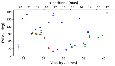
  Figure 15: Linear polarisation EVPAs for feature F1, for the v=1 J=1-0 (blue), v=2 J=1-0 (green) and v=1 J=2-1 (red) SiO maser emission. The lower x-axis shows the channel LSR velocity, and the upper x-axis shows the x-position where the v=1 J=1-0 Stokes parameters were measured, at each velocity channel across the feature. The formal statistical errors are shown for the v=1 J=1-0 and v=2 J=1-0 emission, and the error bars are smaller than the data points in some cases. Additional systematic errors are estimated to be $\leq 5\%$, as discussed in the text.

  The linear polarization EVPA variation across the feature is shown in Figure 15. The two-channel shift discussed in Section 3.2 has been applied to the v=2 J=1-0 data in the Figure. The position angles have a 180^∘ ambiguity, so they were all rotated by integral multiples of 180^∘ to fall within $[0^{\circ},180^{\circ}]$. Error bars are omitted from the v=1 J=2-1 data points to indicate that the absolute values of these angles are uncertain to within a single unknown additive constant offset in the 86 GHz band, as discussed in Section 2. This offset can be selected prudently if it can be physically justified through, for example, alignment with the EVPAs of SiO maser emission from other transitions. In the overlapping region of F1 the EVPAs of all three transitions agree relatively closely, within $\leq 20-30^{\circ}$ (Figure 15). This suggests that the v=1 J=2-1 EVPAs are close to their absolute values, within $\sim 20-30^{\circ}$.

  The v=1 J=1-0 and v=2 J=1-0 error bars in Figure 15 were determined through propagation of the absolute error in the EVPA calibration transfer and the Stokes parameter errors of each maser component, listed in Appendix A. These formal statistical errors do not include systematic errors due to the different angular scales sampled by the VLBA and VLA during the absolute EVPA calibration transfer, or systematic errors arising from source variability during the time delay between the VLA and VLBA observations. The VLBA and VLA observations were separated by 2 days (Section 2). The systematic errors are estimated to be $\leq 5\%$.
  

  Feature F1: v=1 J=2-1

  An EVPA rotation of $\sim 90^{\circ}$ is evident in Figure 15 for the v=1, J=2-1 data near an LSR velocity of 34 km s^-1. However, The rotation is not as abrupt as for feature F2 and neither is it accompanied by the minimum in $m_{l}(\Theta)$ predicted by the GKK solution.
  

  Feature F1: v=1 J=1-0

  The v=1 J=1-0 emission in feature F1 displays what appear to be multiple $\sim 90^{\circ}$ EVPA rotations across the length of the feature.

  These flips may be caused by multiple crossings of the $55^{\circ}$ critical angle, if the feature is elongated along a magnetic field direction oriented close to the critical angle. The v=1 J=1-0 fractional linear polarisation of this feature is $\lesssim 20\%$ (Figure 4). According to the GKK linear polarisation solution (Figure 10), linear polarisation of less than $20\%$ arises over a range of angles $\Theta=48^{\circ}$ to $66^{\circ}$. The three-dimensional position of the feature in the circumstellar envelope is unknown, but for tangential amplification in an accelerating shell we would expect maser emission arising further from the stellar velocity to arise in regions of gas moving at smaller angles to the line of sight. The line of sight velocity of this feature is redshifted by $\sim 11-21$km/s relative to the stellar velocity, so it is possible that this feature is elongated along an axis oriented near $55^{\circ}$ to the line of sight, possibly along a local magnetic field direction.

  Elongation of a feature in the direction of the magnetic field could be caused by ionised gas dragging the magnetic field along the direction of outflow, or a stronger magnetic field may constrain the ionised gas to move along the field lines (Vlemmings et al., 2005; Cotton et al., 2006). Circumstellar maser images often show radially extended features with polarisation position angles either parallel or perpendicular to the radial direction, which have been explained by such alignment with magnetic field lines (Cotton et al., 2006; Kemball et al., 2009).

  The multiple $\sim 90^{\circ}$ rotations visible in the v=1 J=1-0 emission may alternatively be caused by a helical magnetic field threading the elongated maser feature. In this geometry the EVPA would rotate by 180^∘ through the coils of the helix, and there is no need to invoke a transition through the 55^∘ critical angle to explain 90^∘ flips.
  

  The similarity of the total intensity spectral shape in the v=1 J=1-0 and v=1 J=2-1 transitions across F1 shown in Figure 4 suggests strorngly that the emission from these transitions arises from the same physical conditions. However, the measured EVPA values are integrated along the three-dimensional coherent path length of the maser emission, and the maser excitation conditions and SiO density may vary locally in detail across this region. The measured EVPAs are also spatially filtered by the different surface brightness sensitivity of the 43 GHz and 86 GHz arrays. These effects will introduce some level of variance in the emission from different transitions across the feature, even for physically-coincident maser components. In this context, the v=1 J=1-0 and v=1 J=2-1 fractional linear polarisation difference may be explained by modest differences in $\Theta$ between these two transitions, as considered earlier, in Test 1.
  

• Comparison of circular polarisation in the v=1 J=1-0 and J=2-1 transitions.

  A prior comparison of circular polarisation of SiO masers at v=1 J=1-0 and v=1 J=2-1 was performed with a single dish telescope, towards VY CMa, by McIntosh et al. (1994). The circular polarisation was measured for four velocity features in the spectrum. For each velocity feature the v=1 J=1-0 circular polarisation was significantly higher than that in the v=1 J=2-1 transition. In one case the v=1 J=1-0 circular polarisation was measured to be double that of the v=1 J=2-1 circular polarisation, consistent with standard Zeeman splitting, as noted above. As single-dish observations, these prior results are subject to significant but unknown systematic errors arising from spatial blending of individual SiO maser components. Our current study attempts to make this comparison for individual spatially-resolved SiO maser features.

  The circular polarisation was compared for the six overlapping features in the current interferometric component-level study. Of the overlapping features, only F1 and F4 show significant circular polarisation in both the v=1 J=1-0 and v=1 J=2-1 transitions.

  In feature F1, only a single channel displays statistically significant circular polarisation in both transitions: $-4.61\pm 0.30\%$ for v=1 J=1-0, and $-4.31\pm 2.06\%$ for v=1 J=2-1. Standard Zeeman splitting cannot be ruled out for this feature due to the the large uncertainty of the v=1 J=2-1 circular polarisation measurement.

  In the Watson model, saturation effects can increase the standard Zeeman circular polarisation by factors of a few (Watson & Wyld, 2001) so this result could be explained in this model by more highly saturated v=1 J=2-1 emission. This is possible, but not likely, due to the lower intensity of the v=1 J=2-1 line evident in Figure 4.

  Feature F4 is a group of four spots spanning almost 10 km/s (Figure 7). Only spot S1 displays significant circular polarisation in both the v=1 J=1-0 and v=1 J=2-1 lines. The measured fractional circular polarisation of S1 is completely different for the two lines, with a maximum of $9.22\pm 1.31\%$ in the v=1 J=1-0 line, and $-0.84\pm 0.32\%$ in the v=1 J=2-1 line. Closer inspection of the feature shows that the location of the circular polarisation peak of spot S1 is offset between the two lines. The circular polarisation measurements are therefore unlikely to be probing the same region of gas, so this component is not included in the current test.

  The average fractional circular polarisation magnitude across all of the circularly polarised features in Appendix A is 3.0$\%$ for the v=1 J=1-0 line, 4.2$\%$ for the v=2 J=1-0 line, and 2.6$\%$ for the v=1 J=2-1 line. We note however that this is not a comparison between individual coincident components, so is not highly dispositive.
  

• Correlation between circular and linear polarisation.

  Evidence of a circular-linear polarisation correlation has been sought, but not detected, in single dish spectra of VY CMa (McIntosh et al., 1994) as well as VLBA images of v=1 J=1-0 SiO maser emission towards R Aquarii (Boboltz, 1997) and TX Cam (Kemball & Diamond, 1997). In contrast, Herpin et al. (2006) do report a preliminary correlation between integrated circular and linear polarization in a single-dish survey of late-type evolved stars.

  Figure 16 shows circular polarisation percentages versus linear polarisation percentages for maser features with statistically significant linear and circular polarisation. There is no observed correlation between the fractional circular and linear polarisation values.

  There are a total of 37 maser features that display statistically significant linear polarisation in the v=1 J=1-0, v=2 J=1-0 and v=1 J=2-1 feature lists in Appendix A. Of those 37 features, 14 display statistically significant circular polarisation. All of the 14 circularly-polarised features are circularly polarised at a level $>m_{l}^{2}/4$ (Wiebe & Watson, 1998). Another 12 features display circular polarisation without significant linear polarisation. This strongly suggests that the circular polarisation does not arise from non-Zeeman effects, which are described in Section 4.2 Test 6. Cotton et al. (2011) report a similar result from polarised VLBA observations of the AGB star IK Taurii in v=1 J=1-0 and v=2 J=1-0 SiO maser emission.

  

  Figure 16: Plot of fractional circular polarisation magnitude versus fractional linear polarisation magnitude, for the v=1 J=1-0, v=2 J=1-0 and v=1 J=2-1 maser features.

4.4 Magnetic field estimates

If the fractional circular polarisation is generated by the standard Zeeman mechanism, then magnetic field estimates can be derived from the circular polarisation levels. As mentioned previously, the average magnitude of the fractional circular polarisation is 3.0$\%$ for the v=1 J=1-0 line, 4.2$\%$ for the v=2 J=1-0 line, and 2.6$\%$ for the v=1 J=2-1 line. From Elitzur (1996), the magnetic field can be calculated for standard Zeeman circular polarisation, as $B=2\mbox{m}_{c}\Delta v_{5}$ G for J=1-0 SiO maser transitions, where $\Delta v_{5}$ is the Doppler width of the line in units of km/s, fractional circular polarisation $\mbox{m}_{c}$ is taken as a percentage, and adopting $\Theta=45^{\circ}$. The magnetic field relation will be approximately double for the higher frequency J=2-1 transition, $B=2\times 2\mbox{m}_{c}\Delta v_{5}$ G (Elitzur, 1996).

This relation predicts mean magnetic fields of 3.6 and 5.0 G for the v=1 and v=2 J=1-0 lines respectively, and 6.2 G for the v=1 J=2-1 line, assuming a Doppler velocity line-width of 0.6 km/s. Magnetic field estimates from the Watson model will be similar, for standard Zeeman splitting, differing by only a factor of $\sim 2-3$ due to saturation effects (Watson & Wyld, 2001; Watson, 2009).

Similar magnetic field estimates have been reported by Barvainis et al. (1987) and Kemball & Diamond (1997) for SiO maser emission towards a number of late-type evolved stars, assuming standard Zeeman splitting. Barvainis et al. (1987) estimate a magnetic field value of 65 G for VY CMa, which is considerably larger than the magnetic field reported here. The discrepancy is due to their use of a different scale factor in the Zeeman relation than that in the Elitzur (1996) expression used here.

Several magnetic field estimates for VY CMa have also been published for regions at a larger projected radius from the star: $\sim 2$ mG from satellite-line OH maser emission (Cohen et al., 1987), 1 mG from main line OH maser emission (Benson & Mutel, 1982), and $\sim 175-200$ mG from H₂O maser emission (Vlemmings et al., 2002). A magnetic field of order several Gauss is a plausible extrapolation for the SiO maser region, assuming a solar-type $B\propto r^{-2}$ law as a function of radius (Sabin et al., 2015).

If the standard Zeeman derivation of the magnetic field values above is appropriate, then the measured magnetic field values are either sampling a strong global magnetic field, or the masers are preferentially probing regions of locally-enhanced magnetic field with low global filling-factor (Kemball et al., 2009). Figure 3 shows that maser features displaying statistically significant circular polarisation are dispersed throughout the circumstellar envelope. If the circular polarisation is evidence of localised magnetic field enhancements, then the stronger fields appear to be randomly distributed throughout the maser region.

For the elongated feature F1, the v=1 J=1-0 emission displays circular polarisation at a level of $\sim-2$ to $-4\%$ across a region of $\sim 4$ mas in angular extent over the region of the highest total intensity emission in the feature. Using the standard Zeeman interpretation described above, this equates to a magnetic field of $\sim 2$ to 5 G. In that case, the magnetic energy density in the masing gas will exceed the thermal and kinetic energy densities and the magnetic field would have a dominant role in shaping the feature, as suggested by Vlemmings et al. (2005) and Cotton et al. (2006) for other late-type evolved stars. Feature F1 is a long lived maser feature, at least 18 months old (Zhang et al., 2012). If the magnetic field in this feature is as high as the estimates provided by the Zeeman interpretation, then the feature may possibly be located above a highly magnetised outflow above a magnetic cool spot or convective cell.

5 Conclusions

Full-polarisation VLBA images of v=1 J=1-0, v=2 J=1-0 and v=1 J=2-1 SiO masers toward VY CMa were presented. Component-level characteristics of six maser features that are spatially-coincident in more than one transition were used to test maser polarisation models.

The following summary conclusions were reached:

• A comparison of the fractional linear polarisation in the v=1 J=1-0 and v=1 J=2-1 SiO maser emission of the six coincident features showed no clear ordinal relationship with rotational quantum number $J$. This result is more consistent with models predicting spin-independent polarization solutions (Elitzur, 1996).

• An analysis of the dependence of fractional linear polarization on intensity, for the transition v=1 J=1-0, containing the largest number of detected components, proved difficult as a test on saturation effects due to the likely influence of geometric effects evident in the data.

• A trend of stronger fractional linear polarisation closer to the star is not observed, in weak contradiction to the first-order predictions of m-anisotropic pumping models.

• The form of the fractional linear polarisation variation across feature F2 is broadly consistent with a transition across the critical 55^∘ angle $\Theta$ between the magnetic field and the line of sight, as in the GKK model for $m_{l}(\Theta)$ in the parameter regime $g\Omega\gg R\gg\Gamma$ (GKK). However, the limited number of data points across this feature limit the quality of the fit relative to prior results (Kemball et al., 2011). Feature F1 is more complex, displaying multiple $\sim 90^{\circ}$ EVPA rotations and considerably greater fractional linear polarisation in the J=2-1 transition than the J=1-0 transition. The EVPA rotation of the feature may be caused by a helical magnetic field, or orientation close to the $55^{\circ}$ critical angle.

• A component-level comparison of circular polarisation could only be performed for one maser feature (F1) believed to be sampling the same physical conditions in both transitions. In this feature, statistically-significant circular polarisation in the v=1 J=1-0 and v=1 J=2-1 transitions was only observed in one channel across the feature, where the fractional circular polarisation was the same for both transitions, within the measured uncertainties. The large uncertainty in the v=1 J=2-1 fractional circular polarisation measurement means that the standard Zeeman circular polarisation model cannot be ruled out by this single component test.

• The fractional linear and circular polarisation of the maser features were found to be uncorrelated. A significant number of maser features are circularly polarised at a level greater than $m_{l}^{2}/4$, which provides strong evidence against non-Zeeman circular polarisation mechanisms (Wiebe & Watson, 1998).

This work shows that further full polarisation comparisons of J=1-0 and J=2-1 SiO masers are strongly warranted in order to increase the number of coincident components. A larger sample of multi-transition circular polarisation measurements will be especially valuable.

This material is based upon work supported by the National Science Foundation under Grant No. AST 0507473.

Appendix A Maser features

The maser features detected in the v=1 J=2-1, v=1 J=1-0 and v=2 J=1-0 SiO maser transitions are listed in Tables A to LABEL:tab:BR123D1-components. In each table, the columns from left to right are: Velocity $v$, full velocity extent $\Delta v$ of the feature, position offsets $\Delta\alpha$ and $\Delta\delta$ relative to the aligned image centre, Stokes $I$, error in Stokes $I$ $\sigma_{I}$, Stokes $V$, error in Stokes $V$ $\sigma_{V}$, Stokes $Q$, error in Stokes $Q$ $\sigma_{Q}$, Stokes $U$, error in Stokes $U$ $\sigma_{U}$, fractional circular polarisation $m_{c}$, error in fractional circular polarisation $\sigma_{c}$, fractional linear polarisation $m_{l}$, error in fractional linear polarisation $\sigma_{l}$, polarisation position angle $\chi$, error in polarisation position angle $\sigma_{\chi}$. The velocity and Stokes parameters of each feature are measured at the position of the peak Stokes $I$. The units of the Stokes parameters and their uncertainties are Janskys per synthesized beam (Jy/beam). The uncertainties in the Stokes parameters have been empirically broadened as described in the text, and the linear polarisation calculation includes a correction for Ricean bias. The fractional linear and circular polarisation values are presented if they exceed the detection threshold described in the text.

Table 4: List of maser features detected in the v=1 J=2-1 SiO maser transition. The column descriptions are given in the text.

$v$	$\Delta v$	$\Delta\alpha$	$\Delta\delta$	I	$\sigma_{I}$	Q	$\sigma_{Q}$	U	$\sigma_{U}$	V	$\sigma_{V}$	$m_{c}$	$\sigma_{c}$	$m_{l}$	$\sigma_{l}$	$\chi$	$\sigma_{\chi}$
$[$km/s$]$	$[$km/s$]$	$[$mas$]$	$[$mas$]$	$[$Jy/b$]$	$[$Jy/b$]$	$[$Jy/b$]$	$[$Jy/b$]$	$[$Jy/b$]$	$[$Jy/b$]$	$[$Jy/b$]$	$[$Jy/b$]$	$[\%]$	$[\%]$	$[\%]$	$[\%]$	$[$deg$]$	$[$deg$]$
-1.99	0.44	-6.33	-20.64	1.311	0.055	0.014	0.052	0.062	0.051	-0.027	0.053
3.23	3.48	-18.93	-3.93	11.113	0.063	0.071	0.058	0.023	0.061	-0.131	0.059	-1.18	0.53
3.23	2.61	-19.20	5.73	3.308	0.063	-0.040	0.058	0.048	0.061	-0.046	0.059
4.53	0.44	-13.95	-34.44	1.935	0.051	0.005	0.051	0.083	0.050	-0.020	0.049
5.40	1.74	15.30	-0.30	4.117	0.050	-0.026	0.050	0.003	0.049	-0.050	0.051
7.14	1.30	-18.39	-19.92	2.171	0.048	0.042	0.049	0.004	0.048	-0.102	0.050	-4.71	2.29
7.14	0.87	-24.12	0.00	1.897	0.048	-0.101	0.049	0.035	0.048	0.015	0.050
7.57	2.61	-18.69	6.45	2.554	0.047	-0.004	0.050	0.010	0.047	0.014	0.050
8.87	0.87	-19.35	-20.88	1.875	0.056	0.007	0.053	0.026	0.052	-0.043	0.053
8.87	0.87	-26.25	-0.36	1.808	0.056	0.016	0.053	-0.002	0.052	0.042	0.053
9.74	1.30	-16.95	7.11	5.497	0.051	-0.035	0.050	-0.021	0.051	-0.049	0.048
9.74	0.87	-18.63	-2.55	1.900	0.051	-0.021	0.050	0.062	0.051	0.017	0.048
10.18	0.87	-17.76	-3.54	5.643	0.045	-0.014	0.048	0.047	0.049	-0.019	0.046
12.35	1.30	-18.24	-2.94	8.091	0.045	0.059	0.046	-0.061	0.046	-0.142	0.043	-1.76	0.53
13.65	0.87	-18.78	-1.95	2.703	0.055	0.008	0.054	-0.026	0.053	-0.052	0.053
14.09	0.44	33.45	0.36	2.903	0.078	0.031	0.075	0.065	0.074	-0.057	0.073
14.09	0.44	-31.86	3.63	2.255	0.078	-0.064	0.075	0.050	0.074	-0.034	0.073
14.09	0.44	-32.01	-1.11	3.829	0.078	-0.046	0.075	-0.072	0.074	-0.021	0.073
19.30	0.87	20.46	-21.06	1.537	0.061	0.072	0.058	0.065	0.060	0.004	0.060
19.30	0.44	16.65	-23.58	1.046	0.061	-0.069	0.058	0.007	0.060	-0.028	0.060
19.74	0.44	19.14	-24.12	2.575	0.102	0.034	0.101	-0.011	0.102	-0.015	0.101
20.61	1.30	20.43	-24.42	5.166	0.107	0.268	0.101	-0.045	0.104	-0.061	0.102
20.61	2.17	18.33	-23.79	5.595	0.107	-0.026	0.101	0.238	0.104	-0.037	0.102
20.61	0.44	0.24	-22.02	1.568	0.107	-0.033	0.101	-0.008	0.104	0.018	0.102
21.04	1.30	19.86	-25.98	12.601	0.185	-0.626	0.176	-0.099	0.182	-0.193	0.187			4.83	1.14	-85.50	8.94
21.48	0.44	22.08	-24.30	3.641	0.200	-0.018	0.194	-0.117	0.192	-0.092	0.187
21.91	0.87	21.51	-26.58	16.183	0.156	-2.407	0.163	-0.422	0.169	-0.268	0.157			15.07	1.58	-85.03	1.99
22.78	0.44	19.23	-30.21	8.730	0.057	-0.101	0.055	0.045	0.054	-0.128	0.053	-1.46	0.61
23.22	0.44	25.20	-22.17	1.731	0.063	0.002	0.063	-0.067	0.063	-0.046	0.060
24.95	0.44	27.15	-20.76	4.136	0.046	-0.058	0.045	-0.056	0.046	0.007	0.046
26.69	0.44	-8.70	12.69	1.797	0.050	0.023	0.048	0.011	0.049	0.014	0.046
27.13	0.44	-2.46	6.69	1.192	0.071	-0.019	0.070	0.048	0.069	0.014	0.064
27.13	0.44	-8.67	9.96	1.072	0.071	-0.050	0.070	0.018	0.069	-0.054	0.064
27.13	0.44	-23.79	-23.43	3.003	0.071	-0.056	0.070	-0.018	0.069	-0.065	0.064
27.56	0.87	-8.73	8.76	5.864	0.056	-0.009	0.056	0.088	0.056	0.034	0.058
28.43	0.44	1.11	-44.55	1.999	0.059	-0.005	0.060	0.009	0.058	-0.055	0.057
29.30	0.44	12.18	-10.17	1.175	0.060	-0.033	0.059	-0.009	0.059	-0.006	0.062
29.73	1.74	-3.69	5.64	6.151	0.067	0.104	0.065	0.054	0.067	-0.016	0.069
30.17	0.44	-32.49	-19.62	3.033	0.058	0.058	0.057	-0.213	0.055	-0.034	0.055			7.05	0.88	-37.42	7.89
31.04	2.61	-3.93	3.96	7.506	0.142	-0.149	0.145	0.019	0.138	-0.021	0.142
31.04	8.26	-8.37	-25.26	53.815	0.142	-1.694	0.145	-3.012	0.138	-1.187	0.142	-2.21	0.26	6.42	0.48	-59.68	1.19
32.78	1.30	20.64	-14.40	6.326	0.063	-1.866	0.061	-0.081	0.065	0.004	0.062			29.51	1.35	-88.75	1.01
33.64	0.44	-4.92	4.47	1.294	0.056	-0.067	0.059	0.036	0.060	0.015	0.058
34.51	0.44	18.45	-14.22	2.751	0.055	0.380	0.056	0.793	0.055	-0.119	0.057	-4.31	2.06	31.88	1.98	32.20	1.83
34.95	0.44	3.51	-18.03	1.624	0.051	-0.076	0.046	0.041	0.046	0.033	0.049
36.25	0.87	-9.99	-28.35	2.632	0.051	-0.017	0.051	-0.107	0.052	0.084	0.051
37.99	0.44	-10.08	-27.09	1.890	0.042	-0.060	0.041	-0.185	0.040	-0.031	0.041			10.05	0.97	-53.98	6.26
40.16	0.44	-9.12	-18.99	1.796	0.048	-0.032	0.049	-0.032	0.049	-0.037	0.050

Table 5: List of maser features detected in the v=1 J=1-0 SiO maser transition. The column descriptions are given in the text.

Table 6: List of maser features detected in the v=2 J=1-0 SiO maser transition. The column descriptions are given in the text.

References

- Agudo et al. (2010) Agudo I., Thum C., Wiesemeyer H., Krichbaum T. P., 2010, ApJS, 189, 1
- Allen et al. (1989) Allen D. A., Hall P. J., Norris R. P., Troup E. R., Wark R. M., Wright A. E., 1989, MNRAS, 236, 363
- Aller et al. (2003) Aller H. D., Aller M. F., Plotkin R. M., 2003, Ap&SS, 288, 17
- Amiri et al. (2012) Amiri N., Vlemmings W. H. T., Kemball A. J., van Langevelde H. J., 2012, A&A, 538, A136
- Asensio Ramos et al. (2005) Asensio Ramos A., Landi Degl’Innocenti E., Trujillo Bueno J., 2005, ApJ, 625, 985
- Assaf et al. (2013) Assaf K. A., Diamond P. J., Richards A. M. S., Gray M. D., 2013, MNRAS, 431, 1077
- Aurière et al. (2008) Aurière M., et al., 2008, A&A, 491, 499
- Aurière et al. (2010) Aurière M., Donati J., Konstantinova-Antova R., Perrin G., Petit P., Roudier T., 2010, A&A, 516, L2
- Bains et al. (2003) Bains I., Gledhill T. M., Yates J. A., Richards A. M. S., 2003, MNRAS, 338, 287
- Bains et al. (2004) Bains I., Richards A. M. S., Gledhill T. M., Yates J. A., 2004, MNRAS, 354, 529
- Barvainis & Predmore (1985) Barvainis R., Predmore C. R., 1985, ApJ, 288, 694
- Barvainis et al. (1987) Barvainis R., McIntosh G., Predmore C. R., 1987, Nature, 329, 613
- Benson & Mutel (1982) Benson J. M., Mutel R. L., 1982, ApJ, 253, 199
- Boboltz (1997) Boboltz D. A. J., 1997, PhD thesis, Virginia Polytechnic Institute and State University
- Briggs (1995) Briggs D. S., 1995, PhD thesis, New Mexico Institute of Mining and Technology
- Bujarrabal & Nguyen-Q-Rieu (1981) Bujarrabal V., Nguyen-Q-Rieu M., 1981, A&A, 102, 65
- Cernicharo et al. (1993) Cernicharo J., Bujarrabal V., Santaren J. L., 1993, ApJ, 407, L33
- Chapman & Cohen (1986) Chapman J. M., Cohen R. J., 1986, MNRAS, 220, 513
- Clark et al. (1982) Clark F. O., Troland T. H., Johnson D. R., 1982, ApJ, 261, 569
- Clark et al. (1984) Clark F. O., Troland T. H., Pepper G. H., Johnson D. R., 1984, ApJ, 276, 572
- Cohen (1989) Cohen R. J., 1989, Reports on Progress in Physics, 52, 881
- Cohen et al. (1987) Cohen R. J., Downs G., Emerson R., Grimm M., Gulkis S., Stevens G., Tarter J., 1987, MNRAS, 225, 491
- Cotton et al. (2006) Cotton W. D., et al., 2006, A&A, 456, 339
- Cotton et al. (2011) Cotton W. D., Ragland S., Danchi W. C., 2011, ApJ, 736, 96
- Davison & Hinkley (1997) Davison A. C., Hinkley D. V., 1997, Bootstrap Methods and Their Application. Cambridge University Press
- Desmurs et al. (2000) Desmurs J. F., Bujarrabal V., Colomer F., Alcolea J., 2000, A&A, 360, 189
- Diamond & Kemball (2003) Diamond P. J., Kemball A. J., 2003, ApJ, 599, 1372
- Diamond et al. (1994) Diamond P. J., Kemball A. J., Junor W., Zensus A., Benson J., Dhawan V., 1994, ApJ, 430, L61
- Donati et al. (1997) Donati J., Semel M., Carter B. D., Rees D. E., Collier Cameron A., 1997, MNRAS, 291, 658
- Draine (2011) Draine B. T., 2011, Physics of the Interstellar and Intergalactic Medium. Princeton University Press
- Elitzur (1991) Elitzur M., 1991, ApJ, 370, 407
- Elitzur (1992) Elitzur M., 1992, Astronomical Masers. Kluwer Academic Publishers
- Elitzur (1996) Elitzur M., 1996, ApJ, 457, 415
- Elitzur (2002) Elitzur M., 2002, in Migenes V., Reid M. J., eds, IAU Symposium Vol. 206, Cosmic Masers: From Proto-Stars to Black Holes. Astronomical Society of the Pacific, p. 452
- Etoka & Diamond (2004) Etoka S., Diamond P., 2004, MNRAS, 348, 34
- García-Segura et al. (2005) García-Segura G., López J. A., Franco J., 2005, ApJ, 618, 919
- Glassgold & Huggins (1983) Glassgold A. E., Huggins P. J., 1983, MNRAS, 203, 517
- Glenn et al. (2003) Glenn J., Jewell P. R., Fourre R., Miaja L., 2003, ApJ, 588, 478
- Goldreich & Kylafis (1981) Goldreich P., Kylafis N. D., 1981, ApJ, 243, L75
- Goldreich et al. (1973) Goldreich P., Keeley D. A., Kwan J. Y., 1973, ApJ, 179, 111
- Gómez et al. (2009) Gómez Y., Tafoya D., Anglada G., Miranda L. F., Torrelles J. M., Patel N. A., Hernández R. F., 2009, ApJ, 695, 930
- Gray (2003) Gray M. D., 2003, MNRAS, 343, L33
- Gray (2012) Gray M., 2012, Maser Sources in Astrophysics. Cambridge, UK: Cambridge University Press
- Gray & Field (1995) Gray M. D., Field D., 1995, A&A, 298, 243
- Greaves (2002) Greaves J. S., 2002, A&A, 392, L1
- Grunhut et al. (2010) Grunhut J. H., Wade G. A., Hanes D. A., Alecian E., 2010, MNRAS, 408, 2290
- Gustafsson & Höfner (2004) Gustafsson B., Höfner S., 2004, Atmospheres of AGB Stars. In H. J. Habing & H. Olofsson, eds. Asymptotic Giant Branch Stars. Astronomy and Astrophysics Library. Springer New York
- Hall et al. (1990) Hall P. J., Allen D. A., Troup E. R., Wark R. M., Wright A. E., 1990, MNRAS, 243, 480
- Harper & Brown (2006) Harper G. M., Brown A., 2006, ApJ, 646, 1179
- Harper et al. (2001) Harper G. M., Brown A., Lim J., 2001, ApJ, 551, 1073
- Hartquist & Dyson (1997) Hartquist T. W., Dyson J. E., 1997, A&A, 319, 589
- Harwit et al. (2010) Harwit M., et al., 2010, A&A, 521, L51
- Hayya et al. (1975) Hayya J., Armstrong D., Gressis D., 1975, Management Science, 21, 1338
- Heger et al. (2003) Heger A., Fryer C. L., Woosley S. E., Langer N., Hartmann D. H., 2003, ApJ, 591, 288
- Herpin et al. (2006) Herpin F., Baudry A., Thum C., Morris D., Wiesemeyer H., 2006, A&A, 450, 667
- Homan & Lister (2006) Homan D. C., Lister M. L., 2006, AJ, 131, 1262
- Homan & Wardle (2003) Homan D. C., Wardle J. F. C., 2003, Ap&SS, 288, 29
- Homan et al. (2001) Homan D. C., Attridge J. M., Wardle J. F. C., 2001, ApJ, 556, 113
- Houde (2014) Houde M., 2014, ApJ, 795, 27
- Iben & Renzini (1983) Iben I., Renzini A., 1983, ARA&A, 21, 271
- Ireland et al. (2011) Ireland M. J., Scholz M., Wood P. R., 2011, MNRAS, 418, 114
- Kemball (1992) Kemball A. J., 1992, PhD thesis, Rhodes University
- Kemball (1999) Kemball A. J., 1999, in Taylor G. B., Carilli C. L., Perley R. A., eds, Astronomical Society of the Pacific Conference Series Vol. 180, Synthesis Imaging in Radio Astronomy II. Astronomical Society of the Pacific, p. 499
- Kemball & Diamond (1997) Kemball A. J., Diamond P. J., 1997, ApJ, 481, L111
- Kemball & Richter (2011) Kemball A. J., Richter L., 2011, A&A, 533, A26
- Kemball et al. (1995) Kemball A. J., Diamond P. J., Cotton W. D., 1995, A&AS, 110, 383
- Kemball et al. (2009) Kemball A. J., Diamond P. J., Gonidakis I., Mitra M., Yim K., Pan K., Chiang H., 2009, ApJ, 698, 1721
- Kemball et al. (2011) Kemball A. J., Diamond P. J., Richter L., Gonidakis I., Xue R., 2011, ApJ, 743, 69
- Knapp et al. (1995) Knapp G. R., Bowers P. F., Young K., Phillips T. G., 1995, ApJ, 455, 293
- Konstantinova-Antova et al. (2009) Konstantinova-Antova R., Aurière M., Schröder K., Petit P., 2009, in K. G. Strassmeier, A. G. Kosovichev, & J. E. Beckman ed., IAU Symposium Vol. 259, Cosmic Magnetic Fields: From Planets, to Stars and Galaxies. Cambridge University Press, p. 433, doi:10.1017/S1743921309031020
- Leal-Ferreira et al. (2013) Leal-Ferreira M. L., Vlemmings W. H. T., Kemball A., Amiri N., 2013, A&A, 554, A134
- Lèbre et al. (2014) Lèbre A., Aurière M., Fabas N., Gillet D., Herpin F., Konstantinova-Antova R., Petit P., 2014, A&A, 561, A85
- Lipscy et al. (2005) Lipscy S. J., Jura M., Reid M. J., 2005, ApJ, 626, 439
- Matt et al. (2000) Matt S., Balick B., Winglee R., Goodson A., 2000, ApJ, 545, 965
- McIntosh & Predmore (1991) McIntosh A. C., Predmore C. R., 1991, in Haschick A. D., Ho P. T. P., eds, Astronomical Society of the Pacific Conference Series Vol. 16, Atoms, Ions and Molecules: New Results in Spectral Line Astrophysics. Astronomical Society of the Pacific, p. 83
- McIntosh & Predmore (1993) McIntosh G. C., Predmore C. R., 1993, ApJ, 404, L71
- McIntosh et al. (1989) McIntosh G. C., Predmore C. R., Moran J. M., Greenhill L. J., Rogers A. E. E., Barvainis R., 1989, ApJ, 337, 934
- McIntosh et al. (1994) McIntosh G. C., Predmore C. R., Patel N. A., 1994, ApJ, 428, L29
- Monnier et al. (2004) Monnier J. D., et al., 2004, ApJ, 605, 436
- Müller et al. (2005) Müller H. S. P., Schlöder F., Stutzki J., Winnewisser G., 2005, Journal of Molecular Structure, 742, 215
- Nedoluha & Watson (1990a) Nedoluha G. E., Watson W. D., 1990a, ApJ, 354, 660
- Nedoluha & Watson (1990b) Nedoluha G. E., Watson W. D., 1990b, ApJ, 361, L53
- Nedoluha & Watson (1993) Nedoluha G. E., Watson W. D., 1993, in Clegg A. W., Nedoluha G. E., eds, Lecture Notes in Physics Vol. 412, Astrophysical Masers. Springer Berlin / Heidelberg, p. 47
- Nedoluha & Watson (1994) Nedoluha G. E., Watson W. D., 1994, ApJ, 423, 394
- Perley & Taylor (2003) Perley R., Taylor G., 2003, The VLA Calibrator Manual
- Reid (2007) Reid M. J., 2007, in J. M. Chapman & W. A. Baan ed., IAU Symposium Vol. 242, Astrophysical Masers & their Environments. Cambridge University Press, p. 522, doi:10.1017/S1743921307013701
- Reid & Menten (1997) Reid M. J., Menten K. M., 1997, ApJ, 476, 327
- Reid & Moran (1981) Reid M. J., Moran J. M., 1981, ARA&A, 19, 231
- Reid et al. (1979) Reid M. J., Moran J. M., Leach R. W., Ball J. A., Johnston K. J., Spencer J. H., Swenson G. W., 1979, ApJ, 227, L89
- Richards et al. (2004) Richards A. M. S., et al., 2004, in R. Bachiller, F. Colomer, J.-F. Desmurs, & P. de Vicente ed., Proceedings of the 7th EVN Symposium. Observatorio Astronomico Nacional, p. 209 (arXiv:astro-ph/0501028)
- Richter et al. (2013) Richter L., Kemball A., Jonas J., 2013, preprint, (arXiv:1309.2260)
- Sabin et al. (2007) Sabin L., Zijlstra A. A., Greaves J. S., 2007, MNRAS, 376, 378
- Sabin et al. (2015) Sabin L., Wade G. A., Lèbre A., 2015, MNRAS, 446, 1988
- Soker (2000) Soker N., 2000, MNRAS, 312, 217
- Soker & Clayton (1999) Soker N., Clayton G. C., 1999, MNRAS, 307, 993
- Szymczak & Gérard (2004) Szymczak M., Gérard E., 2004, A&A, 423, 209
- Szymczak et al. (1998) Szymczak M., Cohen R. J., Richards A. M. S., 1998, MNRAS, 297, 1151
- Thompson et al. (2004) Thompson A., Moran J., Swenson G. J., 2004, Interferometry and Synthesis in Radio Astronomy, second edn. WILEY-VCH Verlag GmbH & Co. KGaA
- Troland et al. (1979) Troland T. H., Heiles C., Johnson D. R., Clark F. O., 1979, ApJ, 232, 143
- Vitrishchak et al. (2008) Vitrishchak V. M., Gabuzda D. C., Algaba J. C., Rastorgueva E. A., O’Sullivan S. P., O’Dowd A., 2008, MNRAS, 391, 124
- Vlemmings (2007) Vlemmings W. H. T., 2007, in J. M. Chapman & W. A. Baan ed., IAU Symposium Vol. 242, Astrophysical Masers & their Environments. Cambridge University Press, p. 37, doi:10.1017/S1743921307012549
- Vlemmings & van Langevelde (2008) Vlemmings W. H. T., van Langevelde H. J., 2008, A&A, 488, 619
- Vlemmings et al. (2002) Vlemmings W. H. T., Diamond P. J., van Langevelde H. J., 2002, A&A, 394, 589
- Vlemmings et al. (2005) Vlemmings W. H. T., van Langevelde H. J., Diamond P. J., 2005, A&A, 434, 1029
- Vlemmings et al. (2006) Vlemmings W. H. T., Diamond P. J., Imai H., 2006, Nature, 440, 58
- Vlemmings et al. (2012) Vlemmings W. H. T., Ramstedt S., Rao R., Maercker M., 2012, A&A, 540, L3
- Wallin & Watson (1997) Wallin B. K., Watson W. D., 1997, ApJ, 481, 832
- Wardle & Kronberg (1974) Wardle J. F. C., Kronberg P. P., 1974, ApJ, 194, 249
- Watson (1994) Watson W. D., 1994, ApJ, 424, L37
- Watson (2002) Watson W. D., 2002, in V. Migenes & M. J. Reid ed., IAU Symposium Vol. 206, Cosmic Masers: From Proto-Stars to Black Holes. Astronomical Society of the Pacific, p. 464 (arXiv:astro-ph/0107572)
- Watson (2009) Watson W. D., 2009, in A. Esquivel, J. Franco, G. Garcia-Segura, E. de Gouveia Dal Pino, A. Lazarian, S. Lizano & A. Raga ed., Revista Mexicana de Astronomia y Astrofisica Conference Series Vol. 36, Magnetic Fields in the Universe II: from Laboratory and Stars to the Primordial Universe. Instituto de Astronomia, p. 113 (arXiv:0811.1292)
- Watson & Wyld (2001) Watson W. D., Wyld H. W., 2001, ApJ, 558, L55
- Western & Watson (1983) Western L. R., Watson W. D., 1983, ApJ, 275, 195
- Western & Watson (1984) Western L. R., Watson W. D., 1984, ApJ, 285, 158
- Whiting (2012) Whiting M. T., 2012, MNRAS, 421, 3242
- Wiebe & Watson (1998) Wiebe D. S., Watson W. D., 1998, ApJ, 503, L71
- Wittkowski et al. (2011) Wittkowski M., et al., 2011, A&A, 532, L7
- Wittkowski et al. (2012) Wittkowski M., Hauschildt P. H., Arroyo-Torres B., Marcaide J. M., 2012, A&A, 540, L12
- Wong et al. (2016) Wong K. T., Kamiński T., Menten K. M., Wyrowski F., 2016, preprint, (arXiv:1603.03371)
- Zhang et al. (2012) Zhang B., Reid M. J., Menten K. M., Zheng X. W., 2012, ApJ, 744, 23