A Neural Autoregressive Approach to Collaborative Filtering

Abstract

This paper proposes CF-NADE, a neural autoregressive architecture for collaborative filtering (CF) tasks, which is inspired by the Restricted Boltzmann Machine (RBM) based CF model and the Neural Autoregressive Distribution Estimator (NADE). We first describe the basic CF-NADE model for CF tasks. Then we propose to improve the model by sharing parameters between different ratings. A factored version of CF-NADE is also proposed for better scalability. Furthermore, we take the ordinal nature of the preferences into consideration and propose an ordinal cost to optimize CF-NADE, which shows superior performance. Finally, CF-NADE can be extended to a deep model, with only moderately increased computational complexity. Experimental results show that CF-NADE with a single hidden layer beats all previous state-of-the-art methods on MovieLens 1M, MovieLens 10M, and Netflix datasets, and adding more hidden layers can further improve the performance.

1 Introduction

Collaborative filtering (CF) is a class of methods for predicting a user’s preference or rating of an item, based on his/her previous preferences or ratings and decisions made by similar users. CF lies at the core of most recommender systems and has attracted increasing attention along with the recent boom of e-commerce and social network systems. The premise of CF is that a person’s preference does not change much over time. A good CF algorithm helps a user discover products or services that suit his/her taste efficiently.

Generally speaking, there is a dichotomy of CF methods: Memory-based CF and Model-based CF. Memory-based CF usually computes the similarities between users or items directly from the rating data, which are then used for recommendation. The explainatbility of the recommended results as well as the easy-to-implement nature of memory-based CF ensured its popularity in early recommender systems (Resnick et al., 1994). However, memory-based CF has faded out due to its poor performance on real-life large-scale and sparse data.

Distinct from memory-based CF, model-based CF learns a model from historical data and then uses the model to predict preferences of users. The models are usually developed with machine learning algorithms, such as Bayesian networks, clustering models and latent semantic models. Complex preference patterns can be recognized by these models, allowing model-based CF to perform better for preference prediction tasks. Among all these models, matrix factorization is most popular and successful, c.f. (Koren et al., 2009; Salakhutdinov & Mnih, 2008; Mackey et al., 2011; Gopalan et al., 2013).

With the recent development of deep learning (Krizhevsky et al., 2012; Szegedy et al., 2014; He et al., 2015), neural network based CF, a subclass of model-based CF, has gained enormous attention. A prominent example is RBM-based CF (RBM-CF) (Salakhutdinov et al., 2007). RBM-CF is a two-layer undirected generative graph model which generalizes Restricted Boltzmann Machine (RBM) to modeling the distribution of tabular data, such as user’s ratings of movies. RBM-CF has shown its power in Netflix prize challenge. However, RBM-CF suffers from inaccuracy and impractically long training time, since training RBM-CF is intractable and one has to rely on variational approximation or MCMC sampling.

Recently, a good alternative to RBM has been proposed by Larochelle & Murray (2011). The so-called Neural Autoregressive Distribution Estimator (NADE) is a tractable distribution estimator for high dimensional binary vectors. NADE computes the conditional probabilities of each element given the other elements to its left in the binary vector, where all conditionals share the same parameters. The probability of the binary vector can then be obtained by taking the product of these conditionals. Unlike RBM, NADE does not incorporate any latent variable where expensive inference is required, in constrast it can be optimized efficiently by backpropagation. NADE together with its variants achieved competitive results on many machine learning tasks (Larochelle & Lauly, 2012; Uria et al., 2013; Zheng et al., 2014b; Uria et al., 2014; Zheng et al., 2014a, 2015).

In this paper, we propose a novel model-based CF approach named CF-NADE, inspired by RBM-CF and NADE models. Specifically, we will show how to adapt NADE to CF tasks and describe how to improve the performance of CF-NADE by encouraging the model to share parameters between different ratings. We also propose a factored version of CF-NADE to deal with large-scale dataset efficiently. As Truyen et al. (2009) observed, preference usually has the ordinal nature: if the true rating of an item by a user is 3 stars in a 5-star scale, then predicting 4 stars is preferred to predicting 5 stars. We take this ordinal nature of preferences into consideration and propose an ordinal cost to optimize CF-NADE. Moreover, we propose a deep version of CF-NADE, which can be optimized efficiently. The performance of CF-NADE is tested on $3$ real world benchmarks: MovieLens 1M, MovieLens 10M and Netflix dataset. Experimental results show that CF-NADE outperforms all previous state-of-the-art methods.

2 Related Work

As mentioned previously, some of the most successful model-based CF methods are based on matrix factorization (MF) techniques, where a prevalent assumption is that the partially observed matrix is of low rank. In general, MF characterizes both users and items by vectors of latent factors, where the number of factors is much smaller than the number of users or items, and the correlation between user and item factor vectors are used for recommendation tasks. Specifically, Billsus & Pazzani (1998) proposed to apply Singular Value Decomposition (SVD) to CF tasks, which is an early work on MF-based CF. Bias MF (Koren et al., 2009) is proposed to improve the performance of SVD by introducing systematic biases associated with users and items. Mnih & Salakhutdinov (2007) extended MF to a probabilistic linear model with Gaussian noise referred to as Probabilistic Matrix Factorization (PMF), and showed that PMF performed better than SVD. Salakhutdinov & Mnih (2008) proposed a Bayesian treatment of PMF, which can be trained efficiently by MCMC methods. Along this line, Lawrence & Urtasun (2009) proposed a non-linear PMF using Gaussian process latent variable models. There are other MF-based CF methods such as (Rennie & Srebro, 2005; Mackey et al., 2011). Recently, Poisson Matrix Factorization (Gopalan et al., 2014b, a, 2013) was proposed, replacing Gaussian assumption of PMF by Poisson distribution. Lee et al. (2013) extended the low-rank assumption by embedding locality into MF models and proposed Local Low-Rank Matrix Approximation (LLORMA) method, which achieved impressive performance on several public benchmarks.

Another line of model-based CF is based on neural networks. With the tremendous success of deep learning (Krizhevsky et al., 2012; Szegedy et al., 2014; He et al., 2015), neural networks have found profound applications in CF tasks. Salakhutdinov et al. (2007) proposed a variant of Restricted Boltzmann Machine (RBM) for CF tasks, which is successfully applied in Netflix prize challenge (Bennett & Lanning, 2007). Recently, Sedhain et al. (2015) proposed AutoRec, an autoencoder-based CF model, which achieved the state-of-the-art performance on some benchmarks. RBM-CF (Salakhutdinov et al., 2007) and AutoRec (Sedhain et al., 2015) are common in that both of them build different models for different users, where all these models share the parameters. Truyen et al. (2009) proposed to apply Boltzmann Machine (BM) on CF tasks, which extends RBM-CF by integrating the correlation between users and between items. Truyen et al. (2009) also extended the standard BM model so as to exploit the ordinal nature of ratings. Recently, Dziugaite & Roy (2015) proposed Neural Network Matrix Factorization (NNMF), where the inner product between the vectors of users and items in MF is replaced by a feed-forward neural network. However, NNMF does not produce convincing results on benchmarks.

Our proposed method CF-NADE, can be generally categorized as a neural network based CF method. CF-NADE bears some similarities with NADE (Larochelle & Murray, 2011) in that both model vectors with neural autoregressive architectures. The crucial difference between CF-NADE and NADE is that CF-NADE is designed to deal with vectors of variable length, while NADE can only deal with binary vectors of fixed length. Though DocNADE (Larochelle & Lauly, 2012) does take inputs with various lengths, it is designed to model unordered sets of words where each element of the input corresponds to a word, while CF-NADE models user rating vectors, where each element corresponds to the rating to a specific item.

3 NADE for Collaborative Filtering

This section devotes to CF-NADE, a NADE-based model for CF tasks. Specifically, we describe the basic model of CF-NADE in Section 3.1, and propose to improve CF-NADE by sharing parameters between different ratings in Section 3.2. At last, a factored version of CF-NADE is described in Section 3.3 to deal with large-scale datasets.

3.1 The Model

Suppose that there are $M$ items, $N$ users, and the ratings are integers from $1$ to $K$ ($K$-star scale). One practical and prevalent assumption in CF literature is that a user usually rated $D$ items, where $D\ll M$. To tackle sparsity, similar to RBM-CF (Salakhutdinov et al., 2007), we use a different CF-NADE model for each user and all these models share the same parameters. Specifically, all models have the same number of hidden units, but a user-specific model only has $D$ visible units if the user only rated $D$ items. Thus, each CF-NADE has only one single training case, which is a vector of ratings that a user gave to his/her viewed items, but all the weights and biases of these CF-NADE’s are tied.

In this paper, we denote the training case for user $u$ as $\mathbf{r}^{u}=(r^{u}_{m_{o_{1}}},r^{u}_{m_{o_{2}}},\ldots,r^{u}_{m_{o_{D}}})$, where $o$ is a $D$-tuple in the set of permutations of $(1,2,\ldots,D)$ which serves as an ordering of the rated items $m_{i}\in\{1,2,\ldots,M\}$, and $r^{u}_{m_{o_{i}}}\in\{1,2,\ldots,K\}$ denotes the rating that the user gave to item $m_{o_{i}}$. For simplicity, we will omit the index $u$ of ${\bf r}^{u}$, and focus on a single user-specific CF-NADE in the rest of the paper.

CF-NADE models the probability of the rating vector $\bf r$ by the chain rule as:

$$p\left({\bf r}\right)=\prod_{i=1}^{D}p\left(r_{m_{o_{i}}}|{\bf r}_{m_{o_{<i}}}\right)$$ (1)

where ${\bf r}_{m_{o_{<i}}}=(r_{m_{o_{1}}},r_{m_{o_{2}}},\ldots,r_{m_{o_{i-1}}})$ denotes the first $i-1$ elements of $\bf r$ indexed by $o$.

Similar to NADE (Larochelle & Murray, 2011), CF-NADE models the conditionals in Equation 1 with neural networks. To compute the conditionals in Equation 1, CF-NADE first computes the hidden representation of dimension $H$ given ${\bf r}_{m_{o_{<i}}}$ as follows:

$$\mathbf{h}\left({\bf r}_{m_{o_{<i}}}\right)={\bf g}\left(\mathbf{c}+\sum_{j<i}\mathbf{W}^{r_{m_{o_{j}}}}_{:,m_{o_{j}}}\right)$$ (2)

where $\bf g(\cdot)$ is the activation function, such as $\tanh(x)=\frac{\exp(x)-\exp(-x)}{\exp(x)+\exp(-x)}$, ${\bf W}^{k}\in\mathbb{R}^{H\times M}$ is the connection matrix associated with rating $k$, ${\bf W}_{:,j}^{k}\in\mathbb{R}^{H}$ is the $j$^th column of ${\bf W}^{k}$ and $W^{k}_{i,j}$ is an interaction parameter between the $i$^th hidden unit and item $j$ with rating $k$, ${\bf c}\in\mathbb{R}^{H}$ is the bias term.

Then the conditionals in Equation 1 could be modeled as:

$$p\left(r_{m_{o_{i}}}=k|{\bf r}_{m_{o_{<i}}}\right)=\frac{\exp\left(s_{m_{o_{i}}}^{k}\left({\bf r}_{m_{o_{<i}}}\right)\right)}{\sum_{k^{\prime}=1}^{K}\exp\left(s_{m_{o_{i}}}^{k^{\prime}}\left({\bf r}_{m_{o_{<i}}}\right)\right)}$$ (3)

where $s_{m_{o_{i}}}^{k}({\bf r}_{m_{o_{<i}}})$ is the score indicating the preference that the user gave rating $k$ for item $m_{o_{i}}$ given the previous ratings ${\bf r}_{m_{o_{<i}}}$, and $s_{m_{o_{i}}}^{k}({\bf r}_{m_{o_{<i}}})$ is computed as,

$$s_{m_{o_{i}}}^{k}\left({\bf r}_{m_{o_{<i}}}\right)=b^{k}_{m_{o_{i}}}+\mathbf{V}^{k}_{m_{o_{i}},:}\mathbf{h}\left({\bf r}_{m_{o_{<i}}}\right)$$ (4)

where ${\bf V}^{k}\in\mathbb{R}^{M\times H}$ and ${\bf b}^{k}\in\mathbb{R}^{M}$ are the connection matrix and the bias term associated with rating $k$, respectively.

CF-NADE is optimized for minimum negative log-likelihood of $p\left({\bf r}\right)$ (Equation (3)),

$$-\log p\left({\bf r}\right)=-\sum_{i=1}^{D}\log p\left(r_{m_{o_{i}}}|{\bf r}_{m_{o_{<i}}}\right)$$ (5)

averaged over all the training cases. As in NADE, the ordering $o$ in CF-NADE must be predefined and fixed during training for each user. Ideally, the ordering should follow the timestamps when the user gave the ratings. In practice, we find that a ordering that is randomly drawn from the set of permutations of $(1,2,\ldots,D^{u})$ for each user $u$ yields good results. As Uria et al. (2014) observed, we can think of the models trained with different orderings as different instantiations of CF-NADE for the same user. Section 5 will discuss how to (virtually) train a factorial number of CF-NADE’s with different orderings simultaneously, which is the key to extend CF-NADE to a deep model efficiently.

Once the model is trained, given a user’s past behavior $\mathbf{r}=(r_{m_{o_{1}}},r_{m_{o_{2}}},\ldots,r_{m_{o_{D}}})$, the user’s rating of a new item $m^{*}$ can be predicted as

$${\hat{r}}_{m^{*}}=\mathbb{E}_{p\left(r_{m^{*}}=k|{\bf r}\right)}\left[k\right]$$ (6)

where conditional $p\left(r_{m^{*}}=k|{\bf r}\right)$ are computed by Equation 3 along with the hidden representation $\mathbf{h}\left({\bf r}\right)$ and score $s_{m^{*}}^{k}\left({\bf r}\right)$ computed as

$$s_{m^{*}}^{k}\left({\bf r}\right) = b^{k}_{m^{*}}+\mathbf{V}^{k}_{m^{*},:}\mathbf{h}\left({\bf r}\right)$$ (7)

$$\mathbf{h}\left({\bf r}\right) = {\bf g}\left(\mathbf{c}+\sum_{j=1}^{D}\mathbf{W}^{r_{m_{o_{j}}}}_{:,m_{o_{j}}}\right).$$ (8)

3.2 Sharing Parameters Between Different Ratings

In Equations 2 and 4, the connection matrices ${\bf W}^{k}$, ${\bf V}^{k}$ and the bias ${\bf b}^{k}$ are different for different ratings $k$’s. In other words, CF-NADE uses different parameters for different ratings. In practice, for a specific item, some ratings can be much more often observed than others. As a result, parameters associated with a rare rating might not be sufficiently optimized. To alleviate this problem, we propose to share parameters between different ratings of the same item.

Particularly, we propose to compute the hidden representation $\mathbf{h}({\bf r}_{m_{o_{<i}}})$ as follows:

$$\mathbf{h}\left({\bf r}_{m_{o_{<i}}}\right)={\bf g}\left(\mathbf{c}+\sum_{j<i}\sum_{k=1}^{r_{m_{o_{j}}}}\mathbf{W}_{:,m_{o_{j}}}^{k}\right)$$ (9)

Note that, given an item $m_{o_{j}}$ rated $r_{m_{o_{j}}}$ by the user, $\mathbf{h}({\bf r}_{m_{o_{<i}}})$ depends on all the weights ${\bf W}^{k}$, $\forall k\leq r_{m_{o_{j}}}$. Thus, Equation 9 encourages a solution that ${\bf W}^{t}$ is utilized by all the ratings $k$, $\forall k\geq t$.

Similarly, the score $s_{m_{o_{i}}}^{k}({\bf r}_{m_{o_{<i}}})$ in Equation 3 is adjusted as

$$s_{m_{o_{i}}}^{k}\left({\bf r}_{m_{o_{<i}}}\right)=\sum_{j\leq k}\left(b^{j}_{m_{o_{i}}}+\mathbf{V}^{j}_{m_{o_{i}},:}\mathbf{h}\left({\bf r}_{m_{o_{<i}}}\right)\right)$$ (10)

where $\mathbf{V}^{j}$ and ${\bf b}^{j}$ are shared by the rating $k$, where $k\geq j$.

Sharing parameters between different ratings can again be understood as a kind of regularization, which encourages the model to use as many parameters as possible to explain the data. Experimental results in Section 6.2.1 confirm the advantage of this regularization.

3.3 Dealing with Large-Scale Datasets

One disadvantage of CF-NADE we have described so far is that the parameterization of ${\bf W}^{k}\in\mathbb{R}^{H\times M}$ and ${\bf V}^{k}\in\mathbb{R}^{M\times H}$, where $k$ ranges from $1$ to $K$, will result in too many free parameters, especially when dealing with massive datasets. For example, for the Netflix dataset (Bennett & Lanning, 2007), when $H=500$, the number of free parameters by ${\bf W}^{k}$ and ${\bf V}^{k}$ would be around $89$ million. Although severe overfitting can be avoided by proper weight-decay or dropout (Srivastava et al., 2014), learning such a huge network would still be problematic.

Inspired by RBM-CF (Salakhutdinov et al., 2007) and FixationNADE (Zheng et al., 2014a), we propose to address this problem by factorizing ${\bf W}^{k}$ and ${\bf V}^{k}$ into products of two lower-rank matrices. Particularly,

$$W_{i,m}^{k} = \sum_{j=1}^{J}B_{i,j}A_{j,m}^{k}$$ (11)

$$V_{m,i}^{k} = \sum_{j=1}^{J}P_{m,j}^{k}Q_{j,i}$$ (12)

where ${\bf A}^{k}\in\mathbb{R}^{J\times M}$, ${\bf P}^{k}\in\mathbb{R}^{M\times J}$, ${\bf B}\in\mathbb{R}^{H\times J}$ and ${\bf Q}\in\mathbb{R}^{J\times H}$ are lower-rank matrices with $J\ll H$ and $J\ll M$. For example, by setting $J=50$, the number of free parameters for $\bf W$ and $\bf V$ decreases from $89$ million to about $9$ million. In our experiments, this factored version of CF-NADE will be applied on large-scale datasets.

4 Traing CF-NADE with Ordinal Cost

CF-NADE can be trained by minimizing the negative log-likelihood based on conditionals defined by Equation 3. To go one step further, following Truyen et al. (2009), we take the ordinal nature of a user’s preference into consideration. That is, if a user rated an item $k$, the preference of the user to the ratings from $1$ to $k$ should increase monotonically and the preference to the ratings from $k$ to $K$ should decrease monotonically. The basic CF-NADE treats different ratings as separate labels, leaving the ordinal information not captured. Here we describe how to equip CF-NADE with an ordinal cost.

Formally, suppose $r_{m_{o_{i}}}=k$, the ranking of preferences over all the possible ratings under the ordinal assumption can be expressed as:

$$k\succ k-1\succ \ldots \succ 1$$ (13)

$$k\succ k+1\succ \ldots \succ K$$ (14)

where $k\succ k-1$ denotes the preference of rating $k$ over $k-1$, $k\in\{1,2,\ldots,K\}$. Two rankings of ratings, ${\bf y}^{\textup{down}}$ and ${\bf y}^{\textup{up}}$, can be induced by Equation 13 and 14:

$${\bf y}^{\textup{down}} = \left(k,k-1,\ldots,1\right)$$ (15)

$${\bf y}^{\textup{up}} = \left(k,k+1,\ldots,K\right)$$ (16)

Note that maximizing the conditional $p(r_{m_{o_{i}}}=k|{\bf r}_{m_{o_{<i}}})$ in Equation 3 only ensures that the probability of rating $k$ is the largest among all possible ratings. To capture the ordinal nature induced by Equations 13 and 14, we propose to compute the conditional $p(r_{m_{o_{i}}}=k|{\bf r}_{m_{o_{<i}}})$ as

$$p\left(r_{m_{o_{i}}}=k|{\bf r}_{m_{o_{<i}}}\right)=\\ \prod_{j=k}^{1}\frac{\exp(s_{m_{o_{i}}}^{j})}{\sum_{t=1}^{j}\exp(s_{m_{o_{i}}}^{t})}\prod_{j=k}^{K}\frac{\exp(s_{m_{o_{i}}}^{j})}{\sum_{t=j}^{K}\exp(s_{m_{o_{i}}}^{t})}$$ (17)

where $s_{m_{o_{i}}}^{j}$ is a shorthand for the score $s_{m_{o_{i}}}^{j}({\bf r}_{m_{o_{<i}}})$ introduced in Section 3.1, which indicates the preference to rating $k$ of item $m_{o_{i}}$ given the previous context ${\bf r}_{m_{o_{<i}}}$.

Both two products in Equation 17 can be interpreted as the likelihood loss introduced in (Xia et al., 2008) in the context of Listwise Learning To Rank problem. Actually, from the perspective of learning-to-rank, CF-NADE acts as a ranking function which produces rankings of ratings based on previous ratings, where $s_{m_{o_{i}}}^{j}({\bf r}_{m_{o_{<i}}})$ corresponds to the score function in (Xia et al., 2008) and the rankings, ${\bf y}^{\textup{down}}$ and ${\bf y}^{\textup{up}}$, corresponds to true rankings that we would like CF-NADE to fit. Thus, the conditional computed by Equation 17 is actually the conditional distribution of the rankings ${\bf y}^{\textup{down}}$ and ${\bf y}^{\textup{up}}$ given previous $i-1$ ratings. Put differently, the ranking loss in Equation 17 is defined on the ratings, while other learning-to-rank based CF methods, such as (Shi et al., 2010), are on items, which is the crucial difference.

For the rest of the paper, we denote the negative log-likelihood based on the conditionals computed by Equation 17 as ordinal cost $\mathcal{C}_{\textup{ord}}$, and denote the negative log-likelihood based on Equation 3 as regular cost $\mathcal{C}_{\textup{reg}}$. The final cost to optimize the model is then defined as

$$\mathcal{C}_{\textup{hybrid}}=(1-\lambda)\mathcal{C}_{\textup{reg}}+\lambda\mathcal{C}_{\textup{ord}}$$ (18)

where $\lambda$ is the hyperparameter to determine the weight of $\mathcal{C}_{\textup{ord}}$. The impact of the hyperparameter $\lambda$ on the performance of CF-NADE is discussed in Section 6.2.1.

5 Extending CF-NADE to a Deep Model

So far we have described CF-NADE with single hidden layer. As suggested by the recent and impressive success of deep neural networks (Krizhevsky et al., 2012; Szegedy et al., 2014; He et al., 2015), extending CF-NADE to a deep, multiple hidden layers architecture could allow us to have better performance. Recently, Uria et al. (2014) proposed an efficient deep extension to original NADE (Larochelle & Murray, 2011) for binary vector observations, which inspires other related deep model (Zheng et al., 2015). Following (Uria et al., 2014), we propose a deep variant of CF-NADE.

As mentioned in Section 3.1, a different CF-NADE model is used for each user and the ordering $o$ in $\bf r$ is stochastically sampled from the set of permutations of $(1,2,\ldots,D)$. Training CF-NADE on stochastically sampled orderings corresponds, in expectation, to minimizing the cost in Equation 18 over all possible orderings for each user. As noticed by Uria et al. (2014) and Zheng et al. (2015), training over all possible orderings for CF-NADE implies that for any given context ${\bf r}_{{m}_{o_{<i}}}$, the model performs equally well at predicting all the remaining items in ${\bf r}_{{m}_{o_{\geq i}}}$, since for each item there is an ordering such that it appears at position $i$. This is the key observation to extend CF-NADE to a deep model. Specifically, instead of sampling a complete ordering over all the $D$ items, we instead sample a context ${\bf r}_{{m}_{o_{<i}}}$ and perform an update of the conditionals using that context.

The procedure is done as follows. Given a user who has rated $D$ items, an ordering $o$ is first sampled randomly from the set of permutations of $(1,2,\ldots,D)$ for each update and a vector $\mathbf{r}=(r_{m_{o_{1}}},r_{m_{o_{2}}},\ldots,r_{m_{o_{D}}})$ is generated according to the ordering $o$. Then a split point $i$ is randomly drawn from $\{1,2,\dots,D\}$ for each update. The split point $i$ divides ${\bf r}$ into two parts: ${\bf r}_{{m}_{o_{<i}}}$ and ${\bf r}_{{m}_{o_{\geq i}}}$. According to the analysis above, in the new training procedure, ${\bf r}_{{m}_{o_{<i}}}$ is considered as the input of CF-NADE and the training objective is to maximize conditionals $p(r_{m_{o_{j}}}|{\bf r}_{m_{o_{<i}}})$ for each element in ${\bf r}_{{m}_{o_{\geq i}}}$. The cost function with this procedure is

$$\mathcal{C}=\frac{D}{D-i+1}\sum_{j\geq i}-\log p\left(r_{m_{o_{j}}}|{\bf r}_{m_{o_{<i}}}\right).$$ (19)

By Equation 19, the model predicts the ratings of each items after the splitting position $i$ in the randomly drawn ordering $o$ as if it were actually at position $i$. The factors in front of the sum come from the fact that the total number of elements in the sum is $D$ and that we are averaging over $D-i+1$ possible choices for the item at position $i$, similar to (Uria et al., 2014) and (Zheng et al., 2015). Derivation of Equation 19 can be found in the supplementary materials.

In this procedure, a training update relies only on a single hidden representation $\mathbf{h}({\bf r}_{m_{o_{<i}}})$, more hidden layers can be added into CF-NADE with the computational complexity increased moderately. Particularly, suppose $\mathbf{h}^{(1)}({\bf r}_{m_{o_{<i}}})$ is the hidden representation computed in Equation 2. Then new hidden layers can be added as in a regular deep feed-forward neural network:

$$\mathbf{h}^{(l)}\left({\bf r}_{m_{o_{<i}}}\right)={\bf g}\left({\bf c}^{(l)}+{\bf W}^{(l)}{\bf h}^{(l-1)}\left({\bf r}_{m_{o_{<i}}}\right)\right)$$ (20)

for $l=2,\ldots,L$, where $L$ is the total number of hidden layers. Then the conditionals $p(r_{m_{o_{j}}}=k|{\bf r}_{m_{o_{<i}}})$, either in Equation 3 or Equation 17, can be computed from $\mathbf{h}^{(L)}({\bf r}_{m_{o_{<i}}})$. To this end, the number of operations a CF-NADE takes for one input is $O(K\hat{D}H+H^{2}L)$, as in regular multiple layers neural networks, where $\hat{D}$ is the average number of ratings for a user and $H$ is the number of hidden units for each layer. We denote $\tilde{\mathcal{C}}_{\textup{reg}}$ and $\tilde{\mathcal{C}}_{\textup{ord}}$ as the cost functions of Equation 19 associated with conditionals computed by Equation 3 and Equation 17, respectively.

Finally, similar to Equation 18, we can also define a hybrid cost $\tilde{\mathcal{C}}_{\textup{hybrid}}$ as

$$\tilde{\mathcal{C}}_{\textup{hybrid}}=(1-\lambda)\tilde{\mathcal{C}}_{\textup{reg}}+\lambda\tilde{\mathcal{C}}_{\textup{ord}}$$ (21)

Note that CF-NADE with a single hidden layer can also be trained by Equation 19. In practice, Equation 19 can be implemented efficiently on GPUs, hence we use it throughout our experiments for either one hidden layer or multiple-layers architecture.

6 Experiments

In this section, we test the performance of CF-NADE on 3 real-world benchmarks: MovieLens 1M, MovieLens 10M (Harper & Konstan, 2015) and Netflix dataset (Bennett & Lanning, 2007), which contain $10^{6}$, $10^{7}$ and $10^{8}$ ratings, respectively. Following LLORMA (Lee et al., 2013) and AutoRec (Sedhain et al., 2015), $10\%$ of the ratings in each of these datasets are randomly selected as the test set, leaving the remaining $90\%$ of the ratings as the training set. Among the ratings in the training set, $5\%$ are used as validation set. We use a default rating of $3$ for items without training observations. Prediction error is measured by Root Mean Squared Error (RMSE),

$$\textit{RMSE}=\sqrt{\frac{\sum_{i=1}^{S}(r_{i}-\tilde{r}_{i})^{2}}{S}}$$ (22)

where $r_{i}$ is the $i$^th true rating and $\tilde{r}_{i}$ is the predicted rating by the model, $S$ is the total number of ratings in the testset. We report the average RMSE on test set over $5$ different splits and compare CF-NADE with some strong baselines including LLORMA, AutoRec, and other competitive methods. Experimental results show that CF-NADE outperforms the state-of-the-art performance on these benchmarks.

6.1 Datasets Description

MovieLens 1M dataset contains around $1$ million anonymous ratings of approximately $3900$ movies by $6040$ users, where each user rated at least $20$ items. The ratings in MovieLens 1M dataset are made on a $5$-star scale, with $1$-star increments. MovieLen 10M dataset contains about $10$ million ratings of $10681$ movies by $71567$ users. The users of MovieLens 10M dataset are randomly chosen and each user rated at least $20$ movies. Unlike MovieLens 1M dataset, the ratings in MovieLens 10M are on a $5$-star scale with half-star increments. Thus, the number of rating scales of MovieLens 10M is actually $10$. In our experiments, we rescale the ratings in MovieLens 10M to $10$-star scale with $1$-star increments. Netflix dataset comes from the Netflix challenge prize. It is massive compared to the previous two, which contains more than $100$ million ratings of $17770$ movies by $480189$ users. The ratings of Netflix dataset are on $5$-star scale, with $1$-star increments.

6.2 Experiments on MovieLen 1M Dataset

In this section, we test the performance of CF-NADE on MovieLen 1M dataset. We first evaluate the performance of the ordinal cost described in Section 4 with/without sharing parameters between different ratings as described in Section 3.2. Then we compare several variants of CF-NADE with some strong baselines.

6.2.1 The performance of the ordinal cost

In this section, we evaluate the impact of the ordinal weight $\lambda$ in Equation 21 on the performance of CF-NADE. As Sedhain et al. (2015) mentioned, item-based CF outperforms user-based CF, therefore we use item-based CF-NADE (I-CF-NADE) in this section. Distinct from user-based CF-NADE (U-CF-NADE), which builds a different model for each user as we described previously, I-CF-NADE model builds a different CF-NADE model for each item. In other words, the only difference between U-CF-NADE and I-CF-NADE is that the roles of users and items are switched. Comparison between U-CF-NADE and I-CF-NADE can be found in Section 6.2.2.

The configuration of the experiments is as follows. We use a single hidden layer architecture and the number of hidden units is set to $500$, same as AutoRec (Sedhain et al., 2015) and LLORMA (Lee et al., 2013). Adam (Kingma & Ba, 2014) with default parameters ($b_{1}=0.1$,$b_{2}=0.001$ and $\epsilon=10^{-8}$) are utilized to optimize the cost function in Equation 19. The learning rate is set to $0.001$ , the weight decay is set to $0.015$ and we use the tanh activation function.

Let CF-NADE-S denote the variant of CF-NADE model where parameters are shared between different ratings, as described in Section 3.2. Figure 1 shows the superior performance of CF-NADE and CF-NADE-S w.r.t different values of $\lambda$. Effectiveness of parameter sharing and ordinal cost can be justified by observing that: 1) CF-NADE-S always outperforms regular CF-NADE; 2) as the ordinal weight $\lambda$ increases, test RMSE of both CF-NADE and CF-NADE-S decrease monotonically. Based on these observations, we will use CF-NADE-S and fix $\lambda=1$ throughout the rest of the experiments.

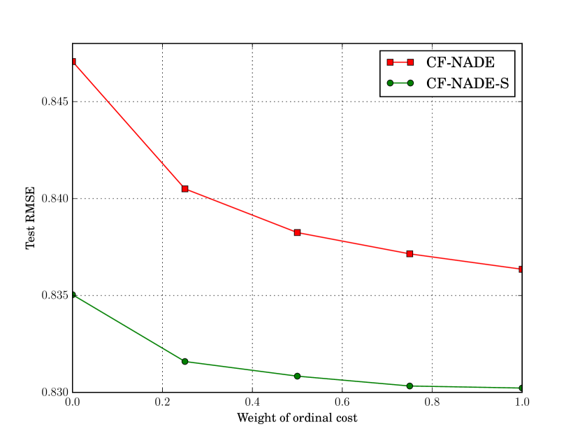
Figure 1: The performance of CF-NADE and CF-NADE-S w.r.t ordinal weight $\lambda$ on MovieLens 1M dataset.

6.2.2 Comparing with strong baselines on MovieLens 1M

In this comparison, we compare CF-NADE with other baselines on MoiveLens 1M dataset. During the comparison, the learning rate is chosen on the validation set by cross-validation among $\{0.001,0.0005,0.0002\}$, and the weight decay is chosen among $\{0.015,0.02\}$. According to Section 6.2.1, the weight $\lambda$ of ordinal cost is fixed to $1$ and CF-NADE-S is adopted. The model is trained with Adam optimizer and tanh as activation function.

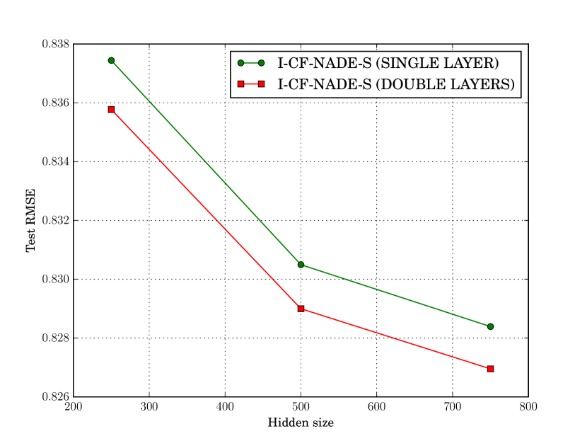
Figure 2: The performance of I-CF-NADE w.r.t the number of hidden units on MovieLens 1M dataset.

Table 1 shows the performance of CF-NADE-S and baselines. The number of hidden units of CF-NADE is $500$, same as AutoRec (Sedhain et al., 2015) for a fair comparison. One can observe that I-CF-NADE-S outperforms U-CF-NADE-S by a large margin. I-CF-NADE-S with a single hidden layer achieves RMSE of $0.830$, which is comparable with any strong baseline. Moreover, I-CF-NADE-S with 2 hidden layers achieves RMSE of $0.829$.

Figure 2 illustrates the performance of I-CF-NADE-S w.r.t the number of hidden units. Increasing the number of hidden units is beneficial, but the return is diminishing. It can also be observed from Figure 2 that deep CF-NADE models achieve better performance than the shallow ones, as expected.

Table 1: Test RMSE of different models on MovieLens 1M.

Method	Test RMSE
PMF$\dagger$	0.883
U-RBM$\ast$	0.881
U-AutoRec (Sedhain et al., 2015)	0.874
LLORMA-Global (Lee et al., 2013)	0.865
I-RBM$\ast$	0.854
BiasMF$\ast$	0.845
NNMF (Dziugaite & Roy, 2015)	0.843
LLORMA-Local (Lee et al., 2013)	0.833
I-AutoRec (Sedhain et al., 2015)	0.831
U-CF-NADE-S (single layer)	0.850
U-CF-NADE-S (2 layers )	0.845
I-CF-NADE-S (single layer)	0.830
I-CF-NADE-S (2 layers)	0.829

$\dagger$: Taken from (Dziugaite & Roy, 2015).
$\ast$: Taken from (Sedhain et al., 2015).

6.3 Experiments on MovieLens 10M Dataset

As mentioned in Section 6.1, the MovieLens 10M is much bigger than the MovieLens 1M, so we opt to use the factored version of CF-NADE described in Section 3.3 and set $J=50$. Even in this setting, I-CF-NADE with $71567$ users and $10$ rating scales will still bring about as many as $70$ million free parameters, Hence, we only report the performance of U-CF-NADE in this experiment. Same as in Section 6.2.1, we train the model with Adam optimizer and using $\mathrm{tanh}$ as activation function. Other configurations are as follows: The number of hidden units to $500$, the weight decay is $0.015$ and $\lambda$ is set to $1$ and parameters are shared between ratings following Section 6.2.1. The base learning rate is $0.0005$, and we double it for the parameters of the first layer.

Table 2 shows the comparison between CF-NADE and other baselines on MovieLens 10M dataset. U-CF-NADE-S with a single hidden layer has already outperformed the baselines, which achieves RMSE of $0.772$. The performance of U-CF-NADE-S can be slightly improved by adding another hidden layer. Noticeably, the test RMSE of U-AutoRec is much worse than I-AutoRec, whereas U-CF-NADE-S outperforms I-AutoRec.

Table 2: Test RMSE of different models on MovieLens 10M.

Method	Test RMSE
U-AutoRec (Sedhain et al., 2015)	0.867
I-RBM$\dagger$	0.825
U-RBM$\dagger$	0.823
LLORMA-Global (Lee et al., 2013)	0.822
BiasMF$\dagger$	0.803
LLORMA-Local (Lee et al., 2013)	0.782
I-AutoRec (Sedhain et al., 2015)	0.782
U-CF-NADE-S (single layer)	0.772
U-CF-NADE-S (2 layers)	0.771

$\dagger$: Taken from (Sedhain et al., 2015).

6.4 Experiments on Netflix Dataset

Our final set of experiments are on the massive Netflix dataset, which contains $10^{8}$ ratings. Similar to Section 6.3, we use the factored version of U-CF-NADE with $J=50$. The Netflix dataset is so big that we need not add a strong regularization to avoid overfitting and therefore set the weight decay to $0.001$. Other configurations are the same as in Section 6.3.

Table 3 compares the performance of U-CF-NADE with other baselines. We can see that U-CF-NADE-S with a single hidden layer achieves RMSE of $0.804$, outperforming all baselines. Another observation from Table 3 is that using a deep CF-NADE architecture achieves a slight improvement over the shallow one, with a test RMSE of $0.803$.

Table 3: Test RMSE of different models on Netflix dataset.

Methods	Test RMSE
LLORMA-Global (Lee et al., 2013)	0.874
U-RBM$\dagger$	0.845
BiasMF$\dagger$	0.844
LLORMA-Local (Lee et al., 2013)	0.834
I-AutoRec (Sedhain et al., 2015)	0.823
U-CF-NADE-S (single layer)	0.804
U-CF-NADE-S (2 layers)	0.803

$\dagger$: Taken from (Sedhain et al., 2015).

Table 4: Complexity of CF-NADE on different benchmarks

Dataset	$\#$Layers	$\#$Params	Train Time	Test Time
		(million)	(second)	(second)
ML 1M	$1$	$30.2$	$3.09$	$0.65$
	$2$	$30.48$	$3.11$	$0.68$
ML 10M	$1$	$10.78$	$134.76$	$31.72$
	$2$	$10.98$	$135.62$	$32.73$
Netflix	$1$	$9.02$	$1057.81$	$239.78$
	$2$	$9.19$	$1064.33$	$243.79$

6.5 The Complexity and Running Time of CF-NADE

We implement CF-NADE using Theano (Bastien et al., 2012) and Blocks (van Merriënboer et al., 2015), and the code is available at https://github.com/Ian09/CF-NADE. Table 4 shows the running time of one epoch as well as the number of parameters used by CF-NADE. For MovieLens 1M dataset, we used the item-based CF-NADE and did not use the factorization method introduced by Sec 3.3, hence the number of parameters for MovieLens 1M is bigger than the other two. Running times in Table 4 include overheads such as transferring data from and to GPU memory for each update. Note that there is still room for faster implementations.

7 Conclusions

In this paper, we propose CF-NADE, a feed-forward, autoregressive architecture for collaborative filtering tasks. CF-NADE is inspired by the seminal work of RBM-CF and the recent advancements of NADE. We propose to share parameters between different ratings to improve the performance. We also describe a factored version of CF-NADE, which reduces the number of parameters by factorizing a large matrix by a product of two lower-rank matrices, for better scalability. Moreover, we take the ordinal nature of preference into consideration and propose an ordinal cost to optimize CF-NADE. Finally, following recent advancements of deep learning, we extend CF-NADE to a deep model with moderate increase of computational complexity. Experimental results on three real-world benchmark datasets show that CF-NADE outperforms the state-of-the-art methods on collaborative filtering tasks. all results of this work rely on explicit feedback, namely, ratings explicitly given by users. however, explicit feedback is not always available or as common as implicit feedback (watch, search, browse behaviors) in real-world recommender systems (Hu et al., 2008). Developing a version of CF-NADE tailored for implicit feedback is left for future work.

References

- Bastien et al. (2012) Bastien, Frédéric, Lamblin, Pascal, Pascanu, Razvan, Bergstra, James, Goodfellow, Ian J., Bergeron, Arnaud, Bouchard, Nicolas, and Bengio, Yoshua. Theano: new features and speed improvements. Deep Learning and Unsupervised Feature Learning NIPS 2012 Workshop, 2012.
- Bennett & Lanning (2007) Bennett, James and Lanning, Stan. The netflix prize. In Proceedings of KDD cup and workshop, volume 2007, pp. 35, 2007.
- Billsus & Pazzani (1998) Billsus, Daniel and Pazzani, Michael J. Learning collaborative information filters. In ICML, volume 98, pp. 46–54, 1998.
- Dziugaite & Roy (2015) Dziugaite, Gintare Karolina and Roy, Daniel M. Neural network matrix factorization. arXiv preprint arXiv:1511.06443, 2015.
- Gopalan et al. (2013) Gopalan, Prem, Hofman, Jake M, and Blei, David M. Scalable recommendation with poisson factorization. arXiv preprint arXiv:1311.1704, 2013.
- Gopalan et al. (2014a) Gopalan, Prem, Ruiz, Francisco JR, Ranganath, Rajesh, and Blei, David M. Bayesian nonparametric poisson factorization for recommendation systems. Artificial Intelligence and Statistics (AISTATS), 33:275–283, 2014a.
- Gopalan et al. (2014b) Gopalan, Prem K, Charlin, Laurent, and Blei, David. Content-based recommendations with poisson factorization. In Advances in Neural Information Processing Systems, pp. 3176–3184, 2014b.
- Harper & Konstan (2015) Harper, F Maxwell and Konstan, Joseph A. The movielens datasets: History and context. ACM Transactions on Interactive Intelligent Systems (TiiS), 5(4):19, 2015.
- He et al. (2015) He, Kaiming, Zhang, Xiangyu, Ren, Shaoqing, and Sun, Jian. Deep residual learning for image recognition. arXiv preprint arXiv:1512.03385, 2015.
- Hu et al. (2008) Hu, Yifan, Koren, Yehuda, and Volinsky, Chris. Collaborative filtering for implicit feedback datasets. In Data Mining, 2008. ICDM’08. Eighth IEEE International Conference on, pp. 263–272. Ieee, 2008.
- Kingma & Ba (2014) Kingma, Diederik and Ba, Jimmy. Adam: A method for stochastic optimization. arXiv preprint arXiv:1412.6980, 2014.
- Koren et al. (2009) Koren, Yehuda, Bell, Robert, and Volinsky, Chris. Matrix factorization techniques for recommender systems. Computer, (8):30–37, 2009.
- Krizhevsky et al. (2012) Krizhevsky, Alex, Sutskever, Ilya, and Hinton, Geoffrey E. Imagenet classification with deep convolutional neural networks. In Advances in neural information processing systems, pp. 1097–1105, 2012.
- Larochelle & Lauly (2012) Larochelle, Hugo and Lauly, Stanislas. A neural autoregressive topic model. In Advances in Neural Information Processing Systems, pp. 2708–2716, 2012.
- Larochelle & Murray (2011) Larochelle, Hugo and Murray, Iain. The neural autoregressive distribution estimator. In International Conference on Artificial Intelligence and Statistics, pp. 29–37, 2011.
- Lawrence & Urtasun (2009) Lawrence, Neil D and Urtasun, Raquel. Non-linear matrix factorization with gaussian processes. In Proceedings of the 26th Annual International Conference on Machine Learning, pp. 601–608. ACM, 2009.
- Lee et al. (2013) Lee, Joonseok, Kim, Seungyeon, Lebanon, Guy, and Singer, Yoram. Local low-rank matrix approximation. In Proceedings of The 30th International Conference on Machine Learning, pp. 82–90, 2013.
- Mackey et al. (2011) Mackey, Lester W, Jordan, Michael I, and Talwalkar, Ameet. Divide-and-conquer matrix factorization. In Advances in Neural Information Processing Systems, pp. 1134–1142, 2011.
- Mnih & Salakhutdinov (2007) Mnih, Andriy and Salakhutdinov, Ruslan. Probabilistic matrix factorization. In Advances in neural information processing systems, pp. 1257–1264, 2007.
- Rennie & Srebro (2005) Rennie, Jasson DM and Srebro, Nathan. Fast maximum margin matrix factorization for collaborative prediction. In Proceedings of the 22nd international conference on Machine learning, pp. 713–719. ACM, 2005.
- Resnick et al. (1994) Resnick, Paul, Iacovou, Neophytos, Suchak, Mitesh, Bergstrom, Peter, and Riedl, John. Grouplens: an open architecture for collaborative filtering of netnews. In Proceedings of the 1994 ACM conference on Computer supported cooperative work, pp. 175–186. ACM, 1994.
- Salakhutdinov & Mnih (2008) Salakhutdinov, Ruslan and Mnih, Andriy. Bayesian probabilistic matrix factorization using markov chain monte carlo. In Proceedings of the 25th international conference on Machine learning, pp. 880–887. ACM, 2008.
- Salakhutdinov et al. (2007) Salakhutdinov, Ruslan, Mnih, Andriy, and Hinton, Geoffrey. Restricted boltzmann machines for collaborative filtering. In Proceedings of the 24th international conference on Machine learning, pp. 791–798. ACM, 2007.
- Sedhain et al. (2015) Sedhain, Suvash, Menon, Aditya Krishna, Sanner, Scott, and Xie, Lexing. Autorec: Autoencoders meet collaborative filtering. In Proceedings of the 24th International Conference on World Wide Web Companion, pp. 111–112. International World Wide Web Conferences Steering Committee, 2015.
- Shi et al. (2010) Shi, Yue, Larson, Martha, and Hanjalic, Alan. List-wise learning to rank with matrix factorization for collaborative filtering. In Proceedings of the fourth ACM conference on Recommender systems, pp. 269–272. ACM, 2010.
- Srivastava et al. (2014) Srivastava, Nitish, Hinton, Geoffrey, Krizhevsky, Alex, Sutskever, Ilya, and Salakhutdinov, Ruslan. Dropout: A simple way to prevent neural networks from overfitting. The Journal of Machine Learning Research, 15(1):1929–1958, 2014.
- Szegedy et al. (2014) Szegedy, Christian, Liu, Wei, Jia, Yangqing, Sermanet, Pierre, Reed, Scott, Anguelov, Dragomir, Erhan, Dumitru, Vanhoucke, Vincent, and Rabinovich, Andrew. Going deeper with convolutions. arXiv preprint arXiv:1409.4842, 2014.
- Truyen et al. (2009) Truyen, Tran The, Phung, Dinh Q, and Venkatesh, Svetha. Ordinal boltzmann machines for collaborative filtering. In Proceedings of the Twenty-fifth Conference on Uncertainty in Artificial Intelligence, pp. 548–556. AUAI Press, 2009.
- Uria et al. (2013) Uria, Benigno, Murray, Iain, and Larochelle, Hugo. Rnade: The real-valued neural autoregressive density-estimator. In Advances in Neural Information Processing Systems, pp. 2175–2183, 2013.
- Uria et al. (2014) Uria, Benigno, Murray, Iain, and Larochelle, Hugo. A deep and tractable density estimator. JMLR: W&CP, 32(1):467–475, 2014.
- van Merriënboer et al. (2015) van Merriënboer, Bart, Bahdanau, Dzmitry, Dumoulin, Vincent, Serdyuk, Dmitriy, Warde-Farley, David, Chorowski, Jan, and Bengio, Yoshua. Blocks and fuel: Frameworks for deep learning. arXiv preprint arXiv:1506.00619, 2015.
- Xia et al. (2008) Xia, Fen, Liu, Tie-Yan, Wang, Jue, Zhang, Wensheng, and Li, Hang. Listwise approach to learning to rank: theory and algorithm. In Proceedings of the 25th international conference on Machine learning, pp. 1192–1199. ACM, 2008.
- Zheng et al. (2015) Zheng, Y., Zhang, Yu-Jin, and Larochelle, H. A deep and autoregressive approach for topic modeling of multimodal data. Pattern Analysis and Machine Intelligence, IEEE Transactions on, PP(99):1–1, 2015. ISSN 0162-8828. doi: 10.1109/TPAMI.2015.2476802.
- Zheng et al. (2014a) Zheng, Yin, Zemel, Richard S, Zhang, Yu-Jin, and Larochelle, Hugo. A neural autoregressive approach to attention-based recognition. International Journal of Computer Vision, 113(1):67–79, 2014a.
- Zheng et al. (2014b) Zheng, Yin, Zhang, Yu-Jin, and Larochelle, H. Topic modeling of multimodal data: An autoregressive approach. In Computer Vision and Pattern Recognition (CVPR), 2014 IEEE Conference on, pp. 1370–1377, June 2014b. doi: 10.1109/CVPR.2014.178.