Correlation transfer in large-spin chains

Abstract

It is shown that transient spin-spin correlations in one-dimensional spin $S\gg 1$ chain can be enhanced for initially factorized and individually squeezed spin states. Such correlation transfer form ”internal” to ”external” degrees of freedom can be well described by using a semiclassical phase-space approach.

I Introduction

Spin chains provide a natural mechanism for creation of quantum channels targeted on correlating of spatially separated particles. State PhysRevLett.70.189 ; bose2007quantu ; PhysRevLett.91.20790 ; horo ; baya and entanglement friedan1986conforma ; subrahmanyam2006transpor ; plenio2004dynamic ; PhysRevA.75.06232 ; PhysRevA.76.05232 ; amico ; osborne2002entangleme transfer can be achieved even in the simplest types of spin chains, which allows to employ them as a medium for a short distance quantum communication. Special attention attracts the idea (recently realized experimentally ex ) of entanglement generation between distant spins venut ; Pop ; yung ; wich ; franco ; wang ; zueco . It was noted bayat2007transfe that while the quality of entanglement transfer in spin chains increases with the dimension of interacting spins, the average fidelity still significantly diminishes with the distance between the spins. In order to enhance the pairewise entanglement we propose to use correlations stored in the initial factorized state of a chain consisting of large size spins. The main idea is to prepare each spin of the chain in an appropriate squeezed state, so that the correlation from the ”internal degree of freedom” is transferred into the spin-spin entanglement during the evolution of the system. It worth noting, that the possibility of correlation transfer between subsystems of various physical systems has been widely discussed both from theoretical C ; cubit ; retama ; wan and experimental exp C ; Dav ; le ; vaz ; barr perspectives.

This article is organized as follows: first we show that for a particular type of spin-spin interaction it is possible to choose an optimal initial spin squeezed state, so that the maximum amount of entanglement between neighbors spins, as well as the correlation of a spin with the rest of the particles in the chain substantially increase; then, we argue that the dynamics of the correlation transfer for large spins can be fairly well described from the semiclassical point of view using the language of the phase-space distributions, which opens the possibility for large-scale simulations of correlation dynamics in spin chains.

II The model

Let us consider an open chain of $N$ spins of size $S$ with homogeneous Ising-like interaction (the coupling constant is taken to be unity), governed by the Hamiltonian

$$H=\sum_{j=1}^{N}S_{z_{j}}S_{z_{j+1}}.$$ (1)

Initially the spins are prepared in a factorized state

$$|\psi_{0}\rangle=\prod\limits_{j=1}^{N}|\psi_{0}\rangle_{j},$$

where each spin is in the coherent state localized on the equator of the Bloch sphere subjected to a squeezing transformation (generated by $S_{z}^{2}$) and a rotation around $x$-axes in the maximum squeezing direction (in the corresponding tangent plane),

$$|\psi_{0}\rangle_{j} = e^{i\vartheta S_{x_{j}}}e^{-i\mu S_{z_{j}}^{2}}|\pi/2,0\rangle_{j},$$ (2)

$$|\pi/2,0\rangle = \frac{1}{2^{s}}\sum\limits_{k=-S}^{S}\sqrt{\frac{2S!}{\left(S-k\right)!\left(S+k\right)!}}|k,S\rangle.$$

Since $|\psi_{0}\rangle$ is not an eigenstate of the Hamiltonian (1) some specific spin-spin correlations arise during the Hamiltonian evolution. The state of the system at time $t$ is

$$|\psi\left(t\right)\rangle=\prod_{j=1}^{N}\sum\limits_{k=-S}^{S}\gamma_{k_{j}}E_{k_{j}}\left(t\right)P_{m,k}^{(j)}\left(\vartheta\right)|m,S\rangle_{j},$$ (3)

where

$$P_{m,k}^{(j)}\left(\vartheta\right) = \,{}_{j}\langle m,S|e^{i\vartheta S_{x}}|k,S\rangle_{j},\quad\gamma_{k}=\frac{1}{2^{S}}\sqrt{\frac{(2S)!}{(S-k)!(S+k)!}},$$

$$E(t)_{k_{j}} = \exp\left(-it\sum_{l}k_{l}m_{l+1}\right)e^{-i\mu k_{j}^{2}}.$$

The simplest characteristics of a correlation between a selected spin and the rest of the spin in the chain is the I-Concurrence PhysRevLett.80.224 ,

$$\mathcal{C}_{I_{j}}=\frac{2S+1}{2S}(1-\mathcal{P}_{j}\left(t\right)),$$ (4)

where $\mathcal{P}_{j}(t)=\mathrm{Tr}(\rho_{j}^{2}(t))$ is the purity of the $j$-th spin. The degree of entanglement between a pair of spins can be described by the negativity PhysRevA.65.032314 ,

$$\mathcal{N}(\rho_{kl})=\frac{2S+1}{2S}(||\rho_{kl}^{tk}||_{1}-1),$$ (5)

where $||\rho||_{1}=Tr\sqrt{\rho\rho^{{\dagger}}}$ is the trace norm of the partially transposed (on the $k$-th spin) reduced two-particle ($k$-$l$) density matrix $\rho_{kl}^{tk}$.

III Optimization of the correlation transfer

We have numerically optimized the $\mathit{I}$-Concurrence with respect to the squeezing parameter $\mu$ and the rotation angle $\vartheta$ for a) a $j$-th spin, $j\neq 1,N$; b) the last (first) spin in the chain.

It results that the optimum squeezing parameter is the same in both cases and scales as $\mu_{opt}\simeq 0.126\ S^{-0.858}$; the optimum rotation angle behaves as $\vartheta_{opt}\simeq\frac{1}{2}\mathrm{arctan}\ {S^{-1/3}}$. For $j$-th spin, $j\neq 1,N$, $\max C_{I_{j}}$ scales with the number of spins in the chain as $\mathcal{\sim}N^{1/5}$ and depends on the size of spins as $\max C_{I_{j}}\simeq A^{g(S)}$, where $A=0.681$ and $g(S)=S^{1/5}$. For the last spins in the chain $\max\mathcal{C}_{I_{1,N}}$ scales with the number of spins as $\sim N^{1/10}$ and depends on the spin size as $\max C_{I_{1,N}}\simeq B^{f(S)}$ where $B=0.523$ and $f(S)=S^{0.191}$. It is worth nothing that the instants, when the maximum value in the $I$-concurrence is reached does not depend nor on the spin size $S$, neither on the longitude of the chain. The dynamics of the $I$-concurrence for the optimized initial spin squeezed (upper curve) and non-squeezed, $\mu=0$, (middle curve) states in case an ”internal” spin is plotted in Fig. (1) and for the last spins of the chain in (2), here $S=5$, $N=6$ .

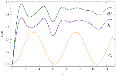
Figure 1: The evolution of the $C_{I_{j}}$ in the chain of 6 spin of size $S=5$. The upper curve corresponds to the optimum squeezing case with $\mu_{opt}=0.5$ and $\vartheta=0.2645$. The middle curve represents non-squeezed initial spin coherent state. The lowest curve is $C_{I_{j}}$ for $S=1/2$. Exact calculations are represented by solid lines and the semi-classical approximation by dotted lines.

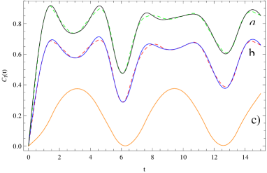
Figure 2: The evolution of the $C_{I_{N}}$ in the chain of 6 spin of size $S=5$. The upper curve correpsonds to the optimum squeezing case with $\mu_{opt}=0.5$ and $\vartheta=0.2643$. The middle curve represents non-squeezed initial spin coherent state. The lowest curve is $C_{I_{N}}$ for $S=1/2$. Exact calculations are represented by solid lines and the semi-classical approximation by dotted lines.

The lowest curve represent the $I$-concurrence for spins-$1/2$. One may observe that a certain improvement of the entanglement between spins is achieved by inducing correlations in the initial factorized state of the system. This effect becomes even more pronounced for internal spins in the limit of large spins $S\gg 1$, when $C_{I_{j}}$ tends to a constant value close to unity.

In the one-fimensional chain (1) the negativity (5) takes non-zero value only for consequtive spins. The negativity $\mathcal{N}_{j,j+1}$ is optimazed for the squeezing parameter $\mu_{opt}\approx 0.856S^{-0.72}$, but scales in a different way for a1) internal pairs and for 2) external pairs, i.e. when one of the spins is located at the end of the chain: in the first case $N_{j,j+1}\sim N^{-0.13}$ and  $N_{j,j+1}\sim D^{h(S)}$, where $D=0.721$ and $h(S)=S^{0.047}$; in the second case $N_{1,2}\sim N^{-0.45}$ and $N_{1,2}\sim G^{r(S)}$, where  $G=0.341$ and $h(S)=S^{0.1}$. The evolution of $N_{j,j+1}$ for the optimized initial spin squeezed (upper curve) and non-squeezed, $\mu=0$, (middle curve) states in case an internal pairs is plotted in Fig. (3) and for the externail pairs (4), here $S=7$, $N=7$.

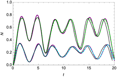
Figure 3: The evolution of $N_{j,j+1}$ for an internal pair, $N=7$, $S=7$. The upper curve correpsonds to the optimum squeezing case with $\mu_{opt}\approx 0.856S^{-0.72}$. The lowest curve represent the evolution without squeezing. Exact calculations are represented by solid lines; the semi-classical approximation using (17) and (18) by dotted and dashed lines correspondingly.

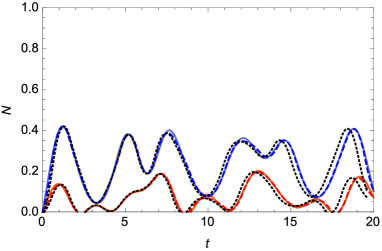
Figure 4: The evolution of $N_{1,2}$, $N=7$, $S=7$. The upper curve correpsonds to the optimum squeezing case with $\mu_{opt}\approx 0.856S^{-0.72}$. The lowest curve represent the evolution without squeezing.Exact calculations are represented by solid lines; the semi-classical approximation using (17) and (18) by dotted and dashed lines correspondingly.

IV Semiclassical approach

Unfortunately, the numerical optimization becomes quite involved for non-diagonal spin chain Hamiltonians and large spin size. In order to be able to carry out such optimization it is appropriate to use the phase-space methods. According to this approach we can reformulate the quantum mechanics on the language of distributions (symbols of operators) in the classical phase-space, where both states and observables are considered as smooth functions in such a way that average values are computed by convoluting symbols of the density matrix and the corresponding operators Wi .

In addition, the quantum dynamics can be efficiently simulated in terms of the spin Wigner function defined as an invertible map of the density matrix $\rho$ to a smooth distribution $W_{\rho}(\Omega)$ on the two-dimensional sphere $\Omega=(\theta,\phi)\in S_{2}$

$$W_{\rho}(\Omega) = \mathrm{Tr}\left(\rho\,\hat{\omega}(\Omega)\right),$$ (6)

$${\rho} {=} \frac{2S+1}{4\pi}\int_{\mathcal{S}_{2}}d\Omega\,\hat{\omega}(\Omega)W(\Omega)$$ (7)

where $\hat{\omega}(\Omega)$ is the kernel operator wigne ,

$$\hat{\omega}(\Omega)=\frac{2\sqrt{\pi}}{\sqrt{2S+1}}\sum_{L=0}^{2S}\sum_{M=-L}^{L}Y_{LM}^{\ast}(\Omega)\hat{T}_{LM}^{(S)},$$ (8)

being $Y_{LM}(\Omega)$ the spherical harmonics and $\hat{T}_{LM}^{(S)}$ the irreducible tensor operators vars .

In the large spin (semiclassical) limit, $S\gg 1$, the Wigner function satisfies the Louville equation klimo ,

$$\partial_{t}\;W_{\rho}(\Omega)=2\epsilon\{W_{\rho}(\Omega),W_{H}(\Omega)\}+O(\epsilon^{3}),$$ (9)

where $\epsilon=(2S+1)^{-1},$ and

$$\{g,f\}=\frac{1}{\mathrm{\sin}\theta}\left(\partial_{\phi}g\partial_{\theta}f-\partial_{\theta}f\partial_{\phi}g\right),$$ (10)

is the Poisson brackets on the sphere, being $W_{H}(\Omega)$ the symbol of the Hamiltonian. The solution of Eq. (9) is just the classical evolution of the initial distribution,

$$W_{\rho}(\Omega|t)=W_{\rho}(\Omega(-t)),$$ (11)

here $\Omega(-t)=(\theta(-t),\phi(-t))$ denotes classical trajectories on the sphere. The mean value of any observable $\hat{f}$ is computed according to

$$\left\langle\hat{f}\right\rangle=\int_{\mathcal{S}_{2}}d\Omega W_{f}(\Omega)W_{\rho}(\Omega).$$ (12)

where $W_{f}(\Omega)$ is the Wigner symbol of $\hat{f}$.
In the case of multi-partite systems the mapping kernel is a product of individual kernels Eq.(8) so that,

$$W_{\rho}\left(\mathbf{\Omega}\right) = Tr\left(\rho\hat{\omega}_{1}(\Omega_{1})...\hat{\omega}_{N}(\Omega_{N})\right),$$ (13)

$$\mathbf{\Omega} \mathbf{=} \mathbf{(}\Omega_{1},...,\Omega_{N}),$$ (14)

and the Wigner function of the reduced bi-partite system of $j$ and $j\prime$ spins has the form

$$W\left(\Omega_{j},\Omega_{j^{\prime}}\right)=\left(\frac{2S+1}{4\pi}\right)^{N-2}\int d\mathbf{\Omega}^{\prime}W_{\rho}\left(\mathbf{\Omega}\right),$$ (15)

where the integration is performed over all spins except for $j$-th and $j\prime$-th. Integrating $W_{\rho}\left(\Omega_{j},\Omega_{j^{\prime}}\right)$ over one of the solid angles one obtaines a single-particle Wigner function, e.g.

$$W\left(\Omega_{j}\right)=\frac{2S+1}{4\pi}\int_{\mathcal{S}_{2}}d\Omega_{j^{\prime}}W\left(\Omega_{j},\Omega_{j^{\prime}}\right).$$ (16)

Taking into account that the symbol of the Hamiltonian Eq.(1) is

$$W_{H}(\mathbf{\Omega})=S(S+1)\sum_{j=1}^{N-1}\mathrm{\cos}\theta_{j}\mathrm{\cos}\theta_{j+1},$$

and solving the equation of motion Eq.(9) one obtains the classical trajectories in the form:
$\theta_{l}=\theta_{l0}$ where $l=1,2,..N$ and

$$\phi_{10} = \phi_{1}-\frac{t}{2\epsilon}\mathrm{\cos}\theta_{2},\quad\phi_{20}=\phi_{2}-\frac{t}{2\epsilon}(\mathrm{\cos}\theta_{1}+\mathrm{\cos}\theta_{3}),$$

$$\quad\phi_{30} = \phi_{3}-\frac{t}{2\epsilon}(\mathrm{\cos}\theta_{2}+\mathrm{\cos}\theta_{4}),...,\phi_{N0}=\phi_{N}-\frac{t}{2\epsilon}\mathrm{\cos}\theta_{N-1}\newline ,$$

here $\theta_{l0}$ and $\phi_{l0}$ stand for the initial values of the corresponding angles. Using the above results we can represent the purity involved in Eq.(4) as follows

$$\mathcal{P}_{j}(t)=\frac{2S+1}{4\pi}\int d\Omega_{j}W^{2}(\Omega_{j},|t).$$

In order to exress the negativity in terms of the Wigner functions we first reconstruct the bi-partite density matrix from (15) and its partially transposed form,

$${\rho}_{jj^{\prime}} {=} \left(\frac{2S+1}{4\pi}\right)^{2}\int d\Omega_{j}d\Omega_{j^{\prime}}W_{\rho}\left(\Omega_{j},\Omega_{j^{\prime}}\right)\hat{\omega}(\Omega_{j})\hat{\omega}(\Omega_{j^{\prime}}),$$

$${\rho}_{jj^{\prime}}^{t_{j}} {=} \left(\frac{2S+1}{4\pi}\right)^{2}\int d\Omega_{j}d\Omega_{j^{\prime}}W_{\rho}\left(\Omega_{j},\Omega_{j^{\prime}}\right)\hat{\omega}^{T}(\Omega_{j})\hat{\omega}(\Omega_{j^{\prime}})$$

and afterwords compute the negativity in accordance with (5),

$$\mathcal{N}_{jj^{\prime}}(t)=\left(\frac{2S+1}{4\pi}\right)^{2}\int W_{\sqrt{\rho^{t1}\rho^{t1{\dagger}}}}(\Omega_{j},\Omega_{j^{\prime}}|t)d\Omega_{j}d\Omega_{j^{\prime}}-1$$ (17)

where $W_{\sqrt{\rho^{t_{j}}\rho^{t_{j}\dagger}}}(\Omega_{j},\Omega_{j^{\prime}})=Tr(\sqrt{\rho_{jj^{\prime}}^{t_{j}}\rho_{jj^{\prime}}^{t_{j}{\dagger}}}\hat{\omega}(\Omega_{j})\hat{\omega}(\Omega_{j^{\prime}}))$.

Curiosly, instead of the complicated expression for the negativity (17) we have found that the following approximation can be used,

$$\mathcal{N}(t)=\int d\Omega_{j}d\Omega_{j^{\prime}}|W^{tj}(\Omega_{j},\Omega_{j^{\prime}}|t)|-1,$$ (18)

where $W^{tj}(\Omega_{j},\Omega_{j^{\prime}})=Tr\left(\rho_{jj^{\prime}}\hat{\omega}^{t}(\Omega_{j})\hat{\omega}(\Omega_{j^{\prime}})\right)$ is the Wigner symbol of the partially transposed density marix. We have tested Eq.(18) for several randomly chosen density matrices.

One of the crucial ingredients of the phase-space approach is that the Wigner function of the initial state can be efficiently approximated in the limit $S\gg 1$ by using the asymptotic form of the mapping kernel wig assym . One can show that the symbol of $j$-th spin state in Eq.(2), $|\psi_{0}\rangle_{j}$, acquires the following approximated form 

$$\small{W_{j}(\Omega)\simeq\sum_{n,k=-S}^{S}\gamma_{k}\gamma_{n}e^{-i\mu(k^{2}-n^{2})-i(n-k)\Phi+\frac{i\pi}{2}(n+k+2S)}d_{nk}^{S}(2\Theta)},$$ (19)

where $d_{nk}^{S}(\Theta)$ is the Wigner $d$-function, and

$$\mathrm{\cos}\Theta = \mathrm{\cos}\theta\ \mathrm{\cos}\vartheta+\mathrm{\sin}\theta\sin\phi\sin\vartheta,$$

$$\mathrm{\sin}\Phi\mathrm{\sin}\Theta = \mathrm{\sin}\theta\sin\phi\cos\vartheta-\mathrm{\cos}\theta\ \mathrm{\sin}\vartheta,$$

which essentially simplifies the simulation of the quantum evolution for large spins.

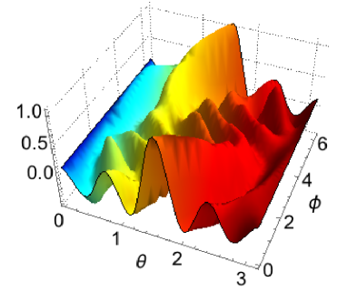
Figure 5: The exact Wigner function of the initial spin state $|\psi_{0}\rangle_{j}$ in Eq.(2).

In Fig.(5) we plot the initial Wigner function, which has a surprisingly non-trivial form (it was verified that the approximate expression Eq. (19) describes well the exact one, Eqs. (6), (8)).

In the Figs. 1 - 2 we compare the quantum (solid line) and the semi-classical (dotted line) dynamics. It is notable that a very good agreement between both types of calculations even for long times is observed. This allows to hope that the problem of optimization of the correlation transfer in more complicated Ising and Heisenberg type large spin chains can be appropriately analyzed by using the semi-classical approach.

Finally, we have shown that an optimization procedure is required in order to the improve the dynamic correlation transfer between different degrees of freedom of large-spin chains. In order to perform such optimization the phase-space methods can be quite useful, especially in the limit of semiclassical-type systems.

References

- (1) C. H. Bennett, G. Brassard, C. Crépeau, R. Jozsa, A. Peres, and W. K. Wootters, Phys. Rev. Lett.70, 1895 (1993).
- (2) S. Bose, Cont. Phys. 48, 13 (2007).
- (3) S. Bose, Phys. Rev. Lett. 91, 207901 (2003).
- (4) M. Horodecki, P. Horodecki, and R. Horodecki, Phys. Rev. A 60, 1888 (1999).
- (5) A. Bayat and S. Bose, Phys. Rev. A 81, 012304 (2010).
- (6) D. Friedan, E. Martinec, and S. Shenker, Nucl. Phys. B 271, 93 (1986).
- (7) V. Subrahmanyam and A. Lakshminarayan, Phys. Lett. A 349, 164 (2006).
- (8) M.B. Plenio, J. Hartley, and J. Eisert, New J. Phys 6, 36 (2004).
- (9) D. Burgarth, V. Giovannetti and S. Bose, Phys. Rev. A 75, 062327 (2007).
- (10) L. C. Venuti, S. M. Giampaolo, F. Illuminati, and P. Zanardi, Phys. Rev. A 76, 052328 (2007).
- (11) L. Amico, R. Fazio, A. Osterloh and V. Vedral, Rev.Mod.Phys. 80, 517 (2008).
- (12) T. J. Osborne and M. A. Nielsen, Phys. Rev. A 66, 032110 (2002).
- (13) S. Sahling, G. Remenyi, C. Paulsen, P. Monceau, V. Saligrama, C. Marin, A. Revcolevschi, L. P. Regnault, S. Raymond and J. E. Lorenzo, Nat. Phys. 11, 255 (2015).
- (14) L.C. Venuti, C.D.E. Boschi, M. Roncaglia, Phys. Rev. Lett. 96, 247206 (2006) ; L.C. Venuti, S.M. Giampaolo, F. Illuminati, P. Zanardi, Phys. Rev. A. 76, 52328 (2007).
- (15) F. Verstraete, M. Popp, and J. I. Cirac, Phys. Rev. Lett. 92, 027901 (2004); L. C. Venuti and M. Roncaglia, Phys. Rev. Lett. 94, 207207 (2005).
- (16) M. H. Yung and S. Bose, Phys. Rev. A 71, 032310 (2005).
- (17) H. Wichterich and S. Bose, Phys. Rev. A 79, 060302(R) (2009).
- (18) C. Di Franco, M. Paternostro, and M. S. Kim, Phys. Rev.A 77, 020303(R) (2008).
- (19) X. Wang, A. Bayat, S. G. Schirmer, and S. Bose, Phys. Rev. A 81, 032312 (2010).
- (20) F. Galve, D. Zueco, S. Kohler, E. Lutz, P. Hanggi, Phys. Rev. A 79, 032332 (2009); F. Galve, D. Zueco, G. M. Reuther, S. Kohler, and P. Hanggi, Europ. Phys. J: Special Topics 180, 237 (2009).
- (21) A. Bayat and V. Karimipour, Phys. Rev. A 75,022321 (2007).
- (22) Z. X. Man, Y. J. Xia and N. B. An, J. Phys. B 44, 095504 (2011); B. Bellomo, et al., Int. J. Quant. Inf. 9, 1665 (2011).
- (23) T. S. Cubitt, F. Verstraete and J. I. Cirac, Phys. Rev. A 71,052308 (2005).
- (24) C. E. López, G. Romero, F. Lastra, E. Solano and J. C. Retamal, Phys. Rev. Lett.101, 080503 (2008).
- (25) Y.-K. Bai, M.-Y. Ye and Z. D. Wang, Phys. Rev. A 80, 044301 (2009).
- (26) L. Lamata, J. León, and D. Salgado, Phys. Rev. A 73, 052325 (2006); E. Nagali, et al. Phys. Rev. Lett. 103, 013601 (2009).
- (27) M.F. Santos, P Milman, L. Davidovich, and N. Zagury, Phys. Rev. A 73, 040305R (2006).
- (28) J. Leach et al., Phys. Rev. Lett. 88, 257901 (2002).
- (29) A. Vaziri et al., Phys. Rev. Lett. 91, 227902 (2003).
- (30) J. T. Barreiro et al., Phys. Rev. Lett. 95, 260501 (2005).
- (31) W. K. Wootters, Phys. Rev. Lett. 80, 2245 (1998).
- (32) G. Vidal, R.F Werner, Phys. Rev A. 65, 032314 (2002).
- (33) J. E. Moyal. Quantum mechanics as a statistical theory (Cambridge Univ Press, 1949).
- (34) P.E Wigner, Phys. Rev. 40, 749 (1932); Hillery M, O. Connel ,M.O Scully and E. P. Wigner, Phys. Rep. 106, 121 (1984); H. W. Lee Phys. Rep. 259, 147 (1995); H. W. Lee, Phys. Rep.259, 147 (1995); C. K. Zachos, D. B. Fairle and T. L. Curtright Quantum mechanics in phase-space (World Scientific, 2005).
- (35) R. L. Stratonovich, Sov. Phys. JETP 31, 1012 (1956); G. S. Agarwal, Phys. Rev. A 24, 2889 (1981); J. C. Várilly and J. M. Gracia-Bondía, Ann. Phys. 190, 107 (1989).
- (36) Varshalovich D A, Moskalev A N and Khersonskiĭ V K 1988 Quantum Theory of Angular Momentum, (World Scientific, Singapore).
- (37) A. B. Klimov, J. Math. Phys. 43 , 2202 (2002); A.B. Klimov and S. M. Chumakov, A Group-Theoretical Approach to Quantum Optics (Wiley-VCH Verlag, Weinheim) (2009)
- (38) A.B. Klimov, S.M. Chumakov, JOSA A 17 2315 (2000)