Plane Pendulum and Beyond by Phase Space Geometry

Abstract

The small angle approximation often fails to explain experimental data, does not even predict if a plane pendulum’s period increases or decreases with increasing amplitude. We make a perturbation ansatz for the Conserved Energy Surfaces of a one-dimensional, parity-symmetric, anharmonic oscillator. A simple, novel algorithm produces the equations of motion and the period of oscillation to arbitrary precision. The Jacobian elliptic functions appear as a special case. Thrift experiment combined with recursive data analysis provides experimental verification of well-known predictions. Development of the quantum/classical analogy enables comparison of time-independent perturbation theories. Many of the useful notions herein generalize to integrable and non-integrable systems in higher dimensions.

I Introduction

Space and time play foundational roles in all experiments and most equations. Measurement of space only requires the definition of a standard length. What difficulties prevent easy measurement of time? A day or year is too long for describing the fall of an apple, while heartbeats depend on unpredictable biological conditions. A pendulum, as in Fig. 1, oscillates through time, setting a scale on the order of one second when $l\approx 1/4(m)$ and $g\approx 9.81(m/s^{2})$.

History credits Galileo with early discoveries regarding the time dependent behavior of oscillating pendulums Ariotti (1968). He noticed the isochrony of identical pendulums, manifest as one characteristic time, the period. Galileo’s initial pronouncement that the period depends not on amplitude now resounds false. The flourishing of classical mechanics provides a logical alternative in perturbation theory. Experiments yielding digital data support predictions contrary to the musings of Galilean renaissance.

The timing of a pendulum does depend on its initial conditionLandau and Lifshitz (1976); Harter (2016). After Legendre and Abel, C.G.J. Jacobi standardized and optimized the solution of the pendulum’s motion by defining a set of elliptic functionsJacobi (1829); Brizard (2009). The Jacobian elliptic functions have many interpretations in physics, but do not fall into the core curriculum because they present serious technical challenges Baker and Bill (2012); Erdös (2000). As an alternative the physics literature contains a variety of approximate solution methods, including: ad hoc Carvalhaes and Suppes (2008); Kidd and Fogg (2002), Lindstedt-Poincaré Landau and Lifshitz (1976); Fulcher and Davis (1976); Park (2012), and canonical perturbation theoryLowenstein (2012).

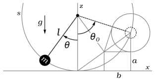
Figure 1: Simple pendulum and coordinate geometry. Half height $a$ determines the period of oscillation.

Our novel method views the pendulum as a one-dimensional, anharmonic oscillator with parity symmetry. In a two-dimensional phase space spanned by position and momentum coordinates, geometric methods apply. Motion happens along a Conserved Energy Surface (C.E.S.), which is not too different from the perimeter of a circle. We make a deformation ansatz and apply an iterative algorithm that sets undetermined functions to force convergence of the energy to one conserved value. One dimensional oscillators are integrable systems, so time dependence follows readily.

The program of derivation involves no mistaken assumptions and refuses temptation to plagiarize standard references. By solving the pendulum equations of motion to high precision, we obtain a series expansion of the Jacobi Elliptic functions $sn(\vartheta,\alpha)$ and $cn(\vartheta,\alpha)$. This exercise distinguishes the derivation as arbitrary-precision and free of error.

A third approximation suffices to describe the pendulum’s motion through one period so long as the motion obeys $\theta\in[-\pi/2,\pi/2]$. A thrift experiment takes place in this range. The setup utilizes a modified USB mouse to produce digital data. Analysis yields extracted parameters that closely agree with carefully derived predictions.

Ultimately we reveal the details of a semiclassical analogy between time-independent perturbation theories. In quantum mechanics approximate wavefunctions must nearly conserve energy. Comparing results for quartic oscillators, we derive a quantum condition, which is equivalent to the Sommerfeld-Wilson prescription in the classical limit.

II Dimensional Analysis

The plane pendulum consists of a massive bob attached by a string or a rod, assumed massless, to an axle as in Fig. 1Harter (2016). Gravity acts on the bob with vertical force $mg$, and the attachment applies a response force, the tension. As time elapses the bob swings and executes a periodic motion along a circular trajectory of radius $l$. In librational motion the sign of $\dot{\theta}$ alternates while the pendulum reaches a maximum deflection $\pm\theta_{0}$ at regular intervals throughout the experiment. The time of one complete oscillation, say from $\theta_{0}$ to $-\theta_{0}$ back to $\theta_{0}$, is called the period.

Table 1 collects the relevant physical quantities, read directly from Fig. 1. Dimensional symbols $[\;L\;]$, $[\;M\;]$, and $[\;T\;]$, denote length, mass, and time. The quantities $\{\sqrt{l/g},\sqrt{a/g},\sqrt{b/g}\}$ all have dimension of time, $[\;T\;]$. Assuming Galileo’s observation correct, $\sqrt{l/g}$ must be the dimensional scale of time because quantities $\{a,b\}$ depend on the amplitude of motion.

Table 1: Dimensional Quantities.

Symbol	Dimension	Trigonometric Form
$l$	$[\;L\;]$	$\cdot$
$a$	$[\;L\;]$	$l\;\sin^{2}(\theta_{0}/2)$
$b$	$[\;L\;]$	$\;\;l\;\sin(\theta_{0}/2)\;\cos(\theta_{0}/2)\;\;$
$g$	$[\;L\;]\;[\;T\;]^{-2}$	$\cdot$
$m$	$[\;M\;]$	$\cdot$

A naive energy argument improves the estimation. The maximum potential energy is $2mga$. Assume that this energy converts entirely to kinetic energy as the mass $m$ moves at constant velocity $2\sqrt{ga}$ through a distance $8b$, then $T_{0}\approx 4b/\sqrt{ga}$. In the small angle approximation, $a\ll l$, $b\approx\sqrt{l\;a}$, and $T_{0}\approx 4\;\sqrt{l/g}$, certainly an underestimate.

The exact period follows from a more sophisticated calculation, again based on conservation of energy. At any half-height $z=(l/2)(1-\cos(\theta))<a$, the kinetic energy equals $2mg(a-z)$, the velocity equals $2\sqrt{g(a-z)}$, and the period equalsLandau and Lifshitz (1976); Brizard (2009)

$$T(a/l) =\int_{0}^{T}dt=4\int_{0}^{l\theta_{0}}\frac{ds}{2\sqrt{g(a-z)}}$$

$$=4\sqrt{\frac{l}{g}}\int_{0}^{\pi/2}\frac{d\xi}{\sqrt{1-(a/l)\sin^{2}(\xi)}}=4\sqrt{\frac{l}{g}}K(\frac{a}{l}),$$

where $ds$ goes along the arc of motion. The complete elliptic integral of the first kind, $K$, admits no simple closed-form. Alternatively, the small angle approximation eliminates dependence on $a$ and gives a concise result

$$T_{0} =\lim\limits_{a\rightarrow 0}4\int_{0}^{2\;b}\frac{dx}{2\sqrt{g(a-z)}}$$

$$=\lim\limits_{a\rightarrow 0}2\sqrt{\frac{l}{g}}\int_{0}^{a}\frac{dz}{\sqrt{z(a-z)}}=2\pi\sqrt{\frac{l}{g}},$$

which requires small-angle identity $s\approx x\approx 2\sqrt{lz}$ to change from the circular line element $ds$ to the horizontal $dx$, and finally to the vertical $dz$. The simple result only applies in the limit $a\rightarrow 0$.

In a general one-dimensional oscillation with small-amplitude period $T_{0}$, we usually have something along the lines

$$T(\alpha,\boldsymbol{\epsilon})=f(\alpha,\boldsymbol{\epsilon})\;T_{0},$$ (3)

with $f(\alpha,\boldsymbol{\epsilon})$ a complicated function of dimensionless energy $\alpha$, and $\boldsymbol{\epsilon}$, structure constants of the potential energy.

With the pendulum experiment the trouble is in the initial conditions. Each initial condition determines one critical parameter

$$\alpha=a/l=\frac{1}{2}\big{(}1-\cos(\theta_{0})\big{)}=\sin^{2}(\theta_{0}/2),$$ (4)

proportional to the total energy. In the simple harmonic approximation $\alpha$ tends to zero as $\theta_{0}^{2}$. Considering this fact, the hypothesis that factor $f(\alpha,\boldsymbol{\epsilon})\rightarrow f(\alpha)$ has a non-terminating power series expansion seems likely. Referencing the expansion of $K(\alpha)$ Research (2016) we have

$$f(\alpha)=\frac{T(\alpha)}{T_{0}}=\frac{2}{\pi}K(\alpha)=\sum_{n=0}^{\infty}\bigg{(}\frac{(2\;n-1)!!}{(2\;n)!!}\bigg{)}^{2}\;\alpha^{n}$$

$$=1+\frac{\alpha}{4}+\frac{9\alpha^{2}}{64}+\frac{25\alpha^{3}}{256}\ldots\;\;\;\;\;\;\;\;\;\;\;\;\;\;\;\;\;\;\;\;\;\;$$ (5)

Numerous approximation schemes (cf. Carvalhaes and Suppes (2008), Table III) aim to simplify the description of a pendulum’s anharmonicity, as measured by coefficients to the powers of $\alpha$. At small $\alpha$ all formulae for $T(\alpha)$ must asymptotically approach Eq.5, so exact and approximate agreement to $\mathcal{O}(\alpha)$ and $\mathcal{O}(\alpha^{2})$ respectively is a common feature of the many published results. For example, the empirical Kidd-Fogg formula Kidd and Fogg (2002) has

$$f(\alpha)=\frac{1}{(1-\alpha)^{1/4}}=1+\frac{\alpha}{4}+\frac{5\alpha^{2}}{32}+\frac{15\alpha^{3}}{128}\ldots$$ (6)

Of course, other factors introduce uncertainty to physical experiments Nelson and Olsson (1986), and these uncertainties always cause the data to deviate from theoretical expectations. Say that we write the standard deviation $\sigma$ in units of $T_{0}$, then $\sigma$ competes in order of magnitude with terms from the expansion of $f(\alpha)$ until eventually, for some integer $n$, we have $c_{n}\;\alpha^{n}\ll\sigma$. This logic is useful in data analysis and gives some restraint to our exploration of approximate solutions.

III Phase Space Geometry

III.1 Small Angle Approximation

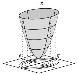
Figure 2: Total Energy Surface. Level sets of the total energy function project trajectories into the plane of phase space, the Conserved Energy Surfaces.

In terms of the phase space coordinates, $(\widetilde{q},\widetilde{p})=(l\;\theta,m\;l\;\dot{\theta})$, the pendulum kinetic and potential energy are

$$T=\widetilde{p}^{2}/2m,\;\;\;\;\;V=m\;g\;l\;(1-\cos(\widetilde{q}/l)).$$ (7)

The potential expands in power series

$$V=m\;g\;l\;\sum_{n=1}\frac{(-1)^{n+1}}{(2n)!}(\widetilde{q}/l)^{2n}.$$ (8)

In the small angle approximation we assume that $\widetilde{q}\ll l$ throughout the experiment. Keeping only the first potential term allows us to write the conserved, total energy of the pendulum oscillator in the small angle approximation

$$E(\alpha)=2\;m\;g\;l\;\alpha\approx\frac{1}{2}(\frac{1}{m}\widetilde{p}^{2}+\frac{m\;g}{l}\widetilde{q}^{2}).$$ (9)

Clearly there exists a bijection between energies and elliptical trajectories, depicted as a projection in Fig. 2. Define radius $\Psi$ and angle $\phi$ the polar coordinates of phase space. Each closed curve $\Psi(\alpha,\phi)\rightarrow\Psi(\alpha)$ is alternatively a phase space trajectory or a Conserved Energy Surface (C.E.S.).

It is much easier to determine time dynamics in a system of measurement where the phase space trajectory takes the particular form of a circle, so we need to apply a canonical transformationRalston (1989)

$$\widetilde{q}\rightarrow q =\bigg{(}\frac{m^{2}\;g}{l}\bigg{)}^{1/4}\;\widetilde{q}\;,$$ (10a)

$$\widetilde{p}\rightarrow p =\bigg{(}\frac{l}{m^{2}\;g}\bigg{)}^{1/4}\;\widetilde{p}\;,$$ (10b)

$$E(\alpha)\rightarrow E(\alpha) =\frac{\omega_{0}}{2}\big{(}p^{2}+q^{2}\big{)},$$ (10c)

with $\omega_{0}=\sqrt{g/l}$. Transformation Eq. 10 takes elliptical trajectories into circular trajectories with equal energy and equal enclosed phase area

$$\lambda(\alpha)=\oint d\widetilde{q}\;\widetilde{p}(\alpha,\widetilde{q})=\oint dq\;p(\alpha,q).$$ (11)

The period

$$T(\alpha)=\oint dt=\oint d\widetilde{q}\;\frac{m}{\widetilde{p}(\alpha,\widetilde{q})}=\oint\frac{dq}{\omega_{0}\;p(\alpha,q)},$$ (12)

also remains invariant under the canonical transformation Eq. 10. To see this we use another definitionArnold (2013) for the period

$$T=\frac{d\lambda}{dE}=\oint dq\bigg{(}\frac{dE}{dp}\bigg{)}^{-1}=\oint\frac{dq}{\omega_{0}\;p},$$ (13)

with $\alpha$ dependence suppressed. This equation proves a connection between the physical period of motion and the purely geometric phase area. As $\lambda(\alpha)$ and $E(\alpha)$ remain invariant under canonical transformation so too must $T(\alpha)$.

Circular trajectories transform invariantly under rotations around the origin of phase space, which immediately implies $\ddot{\phi}=0$. Then the time-dependent solution to the equations of motion is

$$q=\Psi(\alpha,0)\;\cos\big{(}-\omega_{0}(t-t_{0})\big{)},$$ (14a)

$$p=\Psi(\alpha,0)\;\sin\big{(}-\omega_{0}(t-t_{0})\big{)},$$ (14b)

with angular frequency $\omega_{0}=2\;\pi/T_{0}$, $t_{0}$ an arbitrary constant.

The small angle approximation does not say anything about the expansion for $T(\alpha)$. To illustrate the dangers of approximation, let us work out a clever ruse. With $\widetilde{q}\ll l\Longrightarrow l\theta_{0}\approx 2b$ we have

$$\Psi(\alpha,0)^{2} =(\frac{m^{2}g}{l})^{\frac{1}{2}}(2b)^{2}=4\;\beta^{2}\;m\;\sqrt{g\;l^{3}}\;\;\;\;$$

$$=4\;\alpha\;(1-\alpha)\;m\;\sqrt{g\;l^{3}},$$

where $\beta^{2}=(b/l)^{2}=\alpha\;(1-\alpha)$. The constant radius $\Psi(\alpha,0)$ determines the phase area bounded by closed-curve $\Psi(\alpha)$, again assumed circular,

$$\lambda(\alpha) =\oint p(\alpha,q)\;dq=\int_{0}^{2\;\pi}d\phi\int_{0}^{\Psi(\alpha,0)}r\;dr\;\;\;\;\;$$

$$=\pi\;\Psi(\alpha,0)^{2}=\lambda_{0}\;(\alpha-\alpha^{2}),$$

where $\lambda_{0}=2\;m\;g\;l\;T_{0}\;$. We have yet to determine $T(\alpha)$, and do not assume that $T(\alpha)=T_{0}$. Instead we calculate $T(\alpha)$ by the beautiful formula Eq. 13.

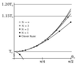
Figure 3: Comparison of Period Approximations. The small angle approximation doesn’t prevent wrong, divergent predictions. Labels for convergent approximations follow naming convention of section IIIB.

Our phase space geometry consists of a triple $\{E,\Psi,\lambda\}$. In the small angle approximation, height $E(\alpha)$ is an exact function of $\alpha$ while perimeter $\Psi(\alpha)$ and area $\lambda(\alpha)$ are merely approximations, so we expect to find inconsistency in the geometry wherever the assumptions break down,

$$f(\alpha)=\frac{1}{T_{0}}\frac{d\alpha}{dE}\frac{d\lambda}{d\alpha}=\frac{1}{\lambda_{0}}\frac{d\lambda}{d\alpha}=(1-2\;\alpha).$$ (17)

Comparing with Eq. 5, we see that $T(\alpha)$ in the small angle approximation may give the wrong $\mathcal{O}(\alpha)$ asymptote as depicted in Fig. 3. Worse, the small angle approximation allows us to predict incorrectly that the period decreases with increasing total energy!

III.2 Simple Anharmonic Approximation

The reductio ad absurdum of section III.A clearly states the need to find a better approximation of the exact phase space geometry. To present results in a more general fashion, we treat the pendulum as an anharmonic oscillator with a potential $V$. The potential expands in power series around a position of stable equilibrium, i.e., $\frac{\partial V}{\partial q}|_{q=0}=0,\frac{\partial^{2}V}{\partial q^{2}}|_{q=0}>0$. Imposing the symmetry constraint $V(q)=V(-q)$, the most general form for the total energy reduces to

$$E=\frac{\omega_{0}}{2}\big{(}p^{2}+q^{2}\big{)}+\sum_{n=1}\frac{\omega_{0}}{(2(n+1))!}\frac{\epsilon_{n}}{\lambda_{\pi}^{n}}q^{2(n+1)},$$ (18)

We make an ansatz of the form

$$\Psi(\alpha,\phi)=\sqrt{2\;\lambda_{\pi}\;\alpha}\;\bigg{(}\;1+\sum_{n}\alpha^{n}\;\psi_{n}(\phi)\;\bigg{)},\;\;\;\;\;$$ (19)

with $\lambda_{\pi}=\frac{\lambda_{0}}{2\;\pi}$.

Our strategy is to substitute $\Psi(\alpha,\phi)$ into the energy equation, and determine the functions $\psi_{n}(\phi)$ in terms of the expansion coefficients $\epsilon_{n}$ by forcing the energy to equal $\lambda_{\pi}\omega_{0}\alpha+\mathcal{O}(\alpha^{N+2})$ for some integer $N\geq 0$. As the C.E.S. more nearly obeys conservation of energy, the approximation improves.

III.2.1 $N=1$, The $\mathcal{O}(\alpha)$ Approximation

A first approximation only requires the first term of each sum in Eqs. 18 & 19. Applying $(q,p)\rightarrow(\Psi(\alpha,\phi)\cos(\phi),\Psi(\alpha,\phi)\sin(\phi))$ to the energy equation and collecting terms by order, we have

$$\alpha\; :\;\lambda_{\pi}\omega_{0}\alpha,$$ (20a)

$$\alpha^{2}\; :\;\lambda_{\pi}\omega_{0}\alpha^{2}\big{(}\frac{\epsilon_{1}}{6}\;\cos(\phi)^{4}+2\;\psi_{1}(\phi)\big{)}.$$ (20b)

Setting terms at $\mathcal{O}(\alpha^{2})$ equal to zero and solving for $\psi_{1}(\phi)$, we find

$$\Psi(\alpha,\phi)=\sqrt{2\;\lambda_{\pi}\;\alpha}\big{(}1-\frac{\epsilon_{1}}{12}\;\alpha\;\cos^{4}(\phi)+\mathcal{O}(\alpha^{2})\big{)}.$$ (21)

As in section III.A. the phase space geometry determines approximate quantities

$$\lambda(\alpha) =\oint p(\alpha,q)\;dq=\int_{0}^{2\;\pi}d\phi\int_{0}^{\psi(\alpha,\phi)}r\;dr\;\;\;\;\;$$

$$=\lambda_{0}\;(\;\alpha-\frac{\epsilon_{1}\;\alpha^{2}}{16})+\mathcal{O}(\alpha^{3}),$$ (22a)

$$f(\alpha) =1-\frac{\epsilon_{1}\;\alpha}{8}+\mathcal{O}(\alpha^{2}).\;\;\;\;$$ (22b)

The pendulum has $\epsilon_{1}=-2$, which makes Eq. 22b asymptotic with Eq. 5 to $\mathcal{O}(\alpha)$.

III.2.2 $N=2$, The $\mathcal{O}(\alpha^{2})$ Approximation

The approximation improves if we include summands for $n=1$ and $n=2$. Evaluation of the energy yields the same constraints as above and

$$\alpha^{3}\; :\;\lambda_{\pi}\omega_{0}\alpha^{3}\big{(}\;\frac{1}{90}\;\epsilon_{2}\;\cos^{6}(\phi)+2\;\psi_{2}(\phi)$$

$$+\frac{2}{3}\;\epsilon_{1}\;\cos^{4}(\phi)\;\psi_{1}(\phi)+\psi_{1}(\phi)^{2}\;\big{)}.$$

Setting $\mathcal{O}(\alpha^{3})$ terms equal to zero, substituting the determined form of $\psi_{1}(\phi)$, and solving for $\psi_{2}(\phi)$ determines

$$\Psi(\alpha,\phi) =\sqrt{2\;\lambda_{\pi}\;\alpha}\big{(}1-\frac{\epsilon_{1}}{12}\;\alpha\;\cos^{4}(\phi)$$

$$+\frac{7\;\epsilon_{1}^{2}}{288}\;\alpha^{2}\;\cos^{8}(\phi)-\frac{\epsilon_{2}}{180}\;\alpha^{2}\;\cos^{6}(\phi)+\mathcal{O}(\alpha^{3})\big{)}.$$

The estimation of $f(\alpha)$ slightly improves,

$$\lambda(\alpha) =\lambda_{0}\;(\alpha-\frac{\epsilon_{1}\;\alpha^{2}}{16}$$ (25a)

$$+\frac{35\;\epsilon_{1}^{2}\;\alpha^{3}}{2304}-\frac{\epsilon_{2}\;\alpha^{3}}{288})+\mathcal{O}(\alpha^{4})$$

$$f(\alpha) =1-\frac{\epsilon_{1}\;\alpha}{8}$$ (25b)

$$+\frac{35\;\epsilon_{1}^{2}\;\alpha^{2}}{768}-\frac{\epsilon_{2}\;\alpha^{2}}{96}+\mathcal{O}(\alpha^{3}).$$

Inserting pendulum values $(\epsilon_{1},\epsilon_{2})=(-2,4)$ makes Eq. 25b asymptotic with Eq. 5 to $\mathcal{O}(\alpha^{2})$.

III.2.3 The $\mathcal{O}(\alpha^{N})$ Approximation

By iterating the procedure applied for $N=1$ and $N=2$, we obtain an approximation to arbitrary order. Every $\psi_{n}(\phi)$ can be expanded in Fourier series or in even powers of cosine. For smooth potentials with a single minimum, the approximation converges according to

$$\lim_{N\rightarrow\infty}E=\lim_{N\rightarrow\infty}\lambda_{\pi}\omega_{0}\alpha+\mathcal{O}(\alpha^{N+2})=\lambda_{\pi}\omega_{0}\alpha.$$ (26)

If the $\boldsymbol{\epsilon}$ coefficients grow rapidly or contain a divergence, then more detailed analysis is required.

A simple symbolic computation calculates higher order expansions by routine. Taking the pendulum as an example with $\epsilon_{n}=(-2)^{n}$, we write a simple code, and store expansion coefficients in the Online Encyclopedia of Integer Sequences Collaboration (2016) (Cf. A273506, A273507, A274130, A274131, A274076, A274078). Relaxing the condition $V(q)=V(-q)$, we also calculate various expansions for a potential where the $\boldsymbol{\epsilon}$ variables take on arbitrary values (Cf. A276738, A276814, A276815, A276816).

Mathematica algorithms available via OEIS entries A273506 and A276816 give two different ways to compute arbitrary precision expansions of phase space trajectories and $K(\alpha)$Klee (2016a). Whenever $N<10$, these algorithms operate in small time on a personal computer. For moderate ranges of $\alpha$, enumeration beyond $N=3$ follows a law of diminishing returns. As can be seen in Fig. 3, the $\mathcal{O}(\alpha^{3})$ approximation already captures to within $1\%$, the exact behavior of the pendulum in the range $\alpha\in[0,1/2]$, $\theta_{0}\in[-\pi/2,\pi/2]$, where our experiment takes place.

III.3 Time Dependence

The phase space trajectory determines time evolution

$$dt=\frac{dq}{\omega_{0}\;p}=\frac{d\phi}{\omega_{0}}\bigg{(}\frac{\Psi^{\prime}(\alpha,\phi)}{\Psi(\alpha,\phi)}\;cot(\phi)-1\bigg{)},$$ (27)

where prime indicates differentiation with respect to $\phi$. Again expand in powers of $\alpha$

$$\frac{\Psi^{\prime}(\alpha,\phi)}{\Psi(\alpha,\phi)}=\alpha\;\psi_{1}^{\prime}(\phi)+\alpha^{2}\;\big{(}\;\psi_{2}^{\prime}(\phi)-$$ (28)

$$\psi_{1}(\phi)\;\psi_{1}^{\prime}(\phi)\;\big{)}+\mathcal{O}(\alpha^{3}),$$

Between two near points in phase space

$$dt \approx\frac{d\phi}{\omega_{0}}\big{(}-1+\frac{1}{3}\;\cos^{4}(\phi)\;\epsilon_{1}\;\alpha$$

$$+(\;\frac{1}{30}\;\cos^{6}(\phi)\;\epsilon_{2}-\frac{1}{6}\;\cos^{8}(\phi)\;\epsilon_{1}^{2}\;)\;\alpha^{2}\;\big{)},$$

where we drop terms higher than $\mathcal{O}(\alpha^{2})$. Expanding cosine terms (Cf. A273496) allows direct integration of $dt$; however, results at high order are not easy to express in concise form. To first order

$$t_{1} =\int_{0}^{t_{1}}dt=-\frac{\phi_{1}}{\omega_{0}}(1-\frac{\epsilon_{1}\;\alpha}{8})$$

$$+\frac{\alpha\;\epsilon_{1}}{\omega_{0}}\big{(}\frac{1}{12}\sin(2\phi_{1})+\frac{1}{96}\sin(4\phi_{1})\big{)}+\mathcal{O}(\alpha^{2}),$$

with limits $\phi(0)=0$ and $\phi(t_{1})=\phi_{1}$. By Lagrange inversion we could in principle obtain $\phi_{1}(t_{1})$ Lang (2016); Whittaker and Watson (1927).

Alternatively, we have

$$\frac{d\phi}{dt}=\dot{\phi}(\phi)=\cos^{2}(\phi)\frac{d}{dt}\bigg{(}\tan(\phi)\bigg{)}.$$ (31)

Using the equations of motion and substituting an approximation for $\frac{d}{dt}\tan(\phi)=(q\dot{p}-\dot{q}p)/q^{2}$, we obtain expressions for the phase space angular velocity, such as

$$\frac{d\phi}{dt}\approx-\omega\bigg{(}\;1+\frac{1}{3}\;\cos^{4}(\phi)\;\epsilon_{1}\;\alpha\;\;\;\;\;\;\;\;\;\;\;\;\;\;\;\;\;\;\;\;\;$$ (32)

$$+\big{(}\frac{1}{30}\;\cos^{6}(\phi)\;\epsilon_{2}-\frac{1}{18}\;\cos^{8}(\phi)\;\epsilon_{1}^{2}\;\big{)}\;\alpha^{2}\;\bigg{)}.$$

The phase velocity $\dot{\phi}$ depends on the phase angle $\phi$, as expected in any oscillation where the phase space trajectory deforms away from elliptical or circular shape. Either limit $(\epsilon_{1},\epsilon_{2})\rightarrow(0,0)$ or $\alpha\rightarrow 0$ recovers constant $\dot{\phi}$, when again trajectories become ellipses or circles.

There are numerous well known methods for calculating numerical time evolution of a Hamiltonian system including symplectic integration Forest and Ruth (1990). In the present case, time evolution occurs along the one-dimensional C.E.S. The standard Runge-Kutta algorithm applies; though, the task of integration requires only minimal complexity. The simple Euler’s method (RK1) suffices. Iteration through time according to $\dot{\phi}$ yields time-dependent predictions, as depicted in Fig. 4. This is the first plot to clearly show anharmonicity as anisochronous motion of pendulums with different initial conditions.

Around $\alpha=0$ all approximations become indistinguishable. To $\alpha=1/2$, the $\mathcal{O}(\alpha)$ approximation closely matches the exact numerical solution, which is nearly indistinguishable from the $\mathcal{O}(\alpha^{3})$ approximation. Isochrony becomes more pronounced at high $\alpha$ where, after $8$ intervals of $\Delta t=T_{0}/8$, the pendulum does not nearly reach its initial condition.

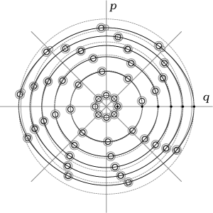
Figure 4: Time Evolution of Pendulums in Phase Space. The $N=10$ ( black ), $N=1$ ( gray ), and circular ( dashed gray ) trajectories are plotted for $\alpha=\{0.01,0.1,0.2,0.3,0.4,0.5\}$. The $N=10$ trajectory completely overlaps the $N=3$ trajectory for all $\alpha$ values, showing convergence. Small filed circles mark initial conditions, while open circles indicate the state of a system at intervals of $\Delta t=T_{0}/8$ as it rotates clock-wise through phase space. Large open circles are calculated by the technique of symplectic integration.

IV Comparison with Standards

IV.1 Jacobian Elliptic Functions

The Jacobian elliptic functions determine exactly the phase space geometry of the simple pendulum. The properties of these functions are well known and recorded in a number of standard resources Abramowitz and Stegun (1964); Whittaker and Watson (1927); Research (2016). Paul Erdös gives a creative, geometric introduction via the Seiffert spiralsErdös (2000).

The exact pendulum phase space trajectory is

$$q(\alpha,\vartheta) =\sqrt{2\;\lambda_{\pi}}\;\arcsin(\sqrt{\alpha}\;sn(\vartheta,\alpha)),$$ (33a)

$$p(\alpha,\vartheta) =\sqrt{2\;\lambda_{\pi}\;\alpha}\;cn(\vartheta,\alpha),$$ (33b)

$$\Psi(\alpha,\vartheta) =\sqrt{q(\alpha,\vartheta)^{2}+p(\alpha,\vartheta)^{2}},$$ (33c)

where $cn$, $sn$ are Jacobian elliptic functions of angular coordinate $\vartheta=K(\alpha)+\omega_{0}\;t$ with period $4K(\alpha)$.

Substituting in time dependence such as Eq. 30, it is possible to expand $\Psi(\alpha,\vartheta)$ in powers of $\alpha$ and prove, order-by-order, equivalence between the exact solution and the approximate solution of III.B. We need not perform this tedious calculation, for any solution that conserves energy must be equivalent to the exact solution. Rather, let us explore convergence by plotting the approximations of $sn$ and $cn$ near the divergence $\alpha=1$.

Setting the left hand side of Eqs. 33a-b equal to an $\mathcal{O}(\alpha^{N})$ approximation allows us to solve for an approximation of both $sn$ and $cn$ Klee (2016a). Composing approximate trajectories $\Psi(\alpha,\phi)$ and time dependence $t(\phi)$ gives parametric function graphs appropriately scaled for comparison, as in Fig. 5.

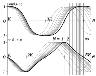
Figure 5: Approximation Around the Divergence. Approximations of $sn$ and $cn$ for $N\in 1,2,3,\ldots 10$ are shown to approach the exact functions, even at $\alpha=0.9$. Vertical lines mark the end of one complete period of the $N^{th}$ approximation.

Once we extend the approximation to functions such as $cn$ and $sn$, it becomes possible to treat other classical motions. We could solve Euler’s equations for the free rotational motion of a rigid bodyLandau and Lifshitz (1976), or describe a photon orbit around a Kerr black holeStein (2016). Using the inversion relationsBrizard (2009); Erdös (2000), we could approximate rotational motion ($\alpha>1$) of a plane pendulum. We follow ErdösErdös (2000) by plotting a couple of Seiffert spiralsSeiffert (1896), as in Fig. 6.

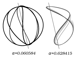
Figure 6: Approximating Seiffert Spirals. For small $\alpha$, $N=1$ approximations closely follow exact Seiffert spirals (left). Approximate trajectories (gray) for $N=1,2,3,\ldots 6$ approach the exact spiral when $\alpha\approx 0.628$ (right). The $N=7$ approximation (black) appears nearly indistinguishable from the exact spiral.

Comparing Figs.  4, 5, and  6 gives an idea of limitations encountered when truncating an arbitrary precision result. In a ”small angle”, even a simple approximation works well. As $\alpha$ becomes large, more terms in the expansion need to be computed. Slow convergence motivates nome expansionsJacobi (1829), useful to know of, but unnecessary in the present context.

IV.2 Alternative Approaches

IV.2.1 Canonical Perturbation Theory

The Hamiltonian formulation of mechanics also allows one to obtain an arbitrary-precision expansion for the phase space trajectory by applying a succession of canonical transformations Lowenstein (2012). The method above is similar in spirit but with a gentle learning curve.

IV.2.2 Mistaken Expansions

A great many authors Landau and Lifshitz (1976); Fulcher and Davis (1976); Park (2012) recommend solving anharmonic oscillations by some variant of the Lindstedt-Poincaré method. This method is error-prone, and usually a wrong assumption is made regarding time dependence (cf. Eq. 30), leading to something like $\psi_{1}(\phi)\propto\cos^{2}(\phi)$ rather than $\psi_{1}(\phi)\propto\cos^{4}(\phi)$. Taking the wrong $\psi_{1}(\phi)$, it is still possible to compute the correct term of the $f(\alpha)$ series expansion, so the mistake often escapes notice.

V Experimental Verification

The experimental setup, procedure, and analysis for determining the period of a plane pendulum are among the most simple and ubiquitous in the physics classroom. A majority of physics students have completed the basic experiment, while relatively few go on to measure amplitude dependence of the period. As is usual in measurement of small perturbations, more stringent precision goals require more sophisticated technology. To make fine measurements of the pendulum’s motion, we need to implement a system with digital data acquisition.

V.1 Setup and Data Processing

Experimental systems are available at cost from manufacturers of scientific classroom equipment, but a USB mouse device Gintautas and Hübler (2009); Peters and Lee (2009) provides a thrifty DIY solution, our preference. After modifying the mouse into a digital pendulum, we connect it to a Linux work station running the X window system Collaboration . The utility program xdotool measures the cursor location directly from the computer’s desktop environment. Integrating with a bash script obtains data at nearly millisecond resolution while the pendulum goes through damping from maximum amplitude to stop, as in Fig.  7.

The oscillation decays through time, only by a small amount per period. Partitioning at zero-amplitude intercepts obtains a division of the amplitude vs. time data into a number of non-overlapping, nearly-sinusoidal samples of one-period duration. Averaging maximum and minimum amplitude, we then associate one-to-one a set of periods and a set of amplitudes. Converting amplitude to energy yields a set of period vs. energy values. Repeating this process for 100 separate trials, we obtain a dense sample, as in Fig.  7.

The bulk data obviously shows significant noise, but the sheer number of data points, more than $2000$, enables noise reduction by a procedure of binning and averaging. We set meta-analysis parameters for bin width $\Delta\alpha$ and a minimum energy cutoff $\alpha_{min}$ to obtain a more manageable data set, with no apparent noise problem.

V.2 Recursive Data Analysis

Of course we are not the first to obtain digital pendulum data, or even the first to analyze amplitude dependence Lewowski and Wozniak (2002); Nicklin and Rafert (1984); S. Gil and Gregorio (2008). We fit $K(\alpha)$ using the period as a free parameter and observe good agreement over the data range, as in previous investigations. To determine just how well $K(\alpha)$ describes the data requires a novel analysis.

It should be possible to extract expansion coefficients by fitting a cubic function to the data, but immediately we encounter a covariance problem. The slope of the data does not change sign, remains nearly flat. One pass analysis yields inaccurate parameter estimation, a wide range of plausible fits.

To improve accuracy and precision we take advantage of the data’s asymptotic nature by partitioning the entire set into three simply connected, disjoint subsets. This introduces two additional analysis priors, energy values, $\alpha_{LQ}$ and $\alpha_{QC}$, which demarcate boundaries as in Fig.  7. The fit procedure first determines the period and linear expansion coefficient from linear data, subsequently determines the quadratic expansion coefficient from the union of linear and quadratic data, finally determines the cubic expansion coefficient from all data.

In total, the analysis depends on four meta-analysis parameters: $\{\alpha_{min},\Delta\alpha,\alpha_{LQ},\alpha_{QC}\}$. To set these values we adopt the following heuristics:

• Use as much data as possible.

• Exclude noisy data around $\alpha=0$.

• Make the bin width as small as possible.

• Capture at least 10 data points per bin.

• In the linear range $[0,\alpha_{LQ}]$:

  $$\frac{2}{\pi}K(\alpha)-(1+\frac{1}{4}\alpha)<0.001\times\frac{2}{\pi}K(\alpha).$$

• In the quadratic range $[0,\alpha_{QC}]$:

  $$\frac{2}{\pi}K(\alpha)-(1+\frac{1}{4}\alpha+\frac{9}{64}\alpha^{2})<0.001\times\frac{2}{\pi}K(\alpha).$$

• The extracted linear, quadratic, cubic coefficients should have increasing uncertainty.

• Minimize uncertainty where possible.

From these we have initial values $\{\alpha_{min},\Delta\alpha,\alpha_{LQ},\alpha_{QC}\}=\{0.003,0.013,0.083,0.21\}$. Searching around, not too far, we find the best fit of Table 2. Comparison of extracted parameters with coefficients of Eq. 6 leads to the humorous conclusion that the Kidd-Fogg formula—though false de facto—also adequately fits the data. That is, the cubic fit does not distinguish between competing Eqs.5-6. To decide against Kidd-Fogg by data alone requires an experiment with sufficient quality up to and beyond $\alpha=0.6$, i.e. $5-10$ expansion coefficients of $K(\alpha)$.

Table 2: Cubic Best Fit Parameters.

$\{\alpha_{min},\Delta\alpha,\alpha_{LQ},\alpha_{QC}\}=\{0.003,0.013,0.08,0.22\}$    Expectation        Estimate       Error $\frac{1}{4}\approx 0.2500$ $0.2463\pm 0.0071$ $0.52\sigma\;,\;1.5\%$ $\frac{9}{64}\approx 0.1406$ $0.1508\pm 0.0082$ $1.24\sigma\;,\;7.2\%$ $\frac{25}{256}\approx 0.0977$ $0.1037\pm 0.0126$ $0.48\sigma\;,\;6.2\%$

Choosing other vales for $\{\alpha_{min},\Delta\alpha,\alpha_{LQ},\alpha_{QC}\}$ we obtain similar best fit parameters, especially when heuristics are nearly obeyed. To facilitate comparison of various analyses, archival data and basic tools are available onlineKlee (2016b, c).

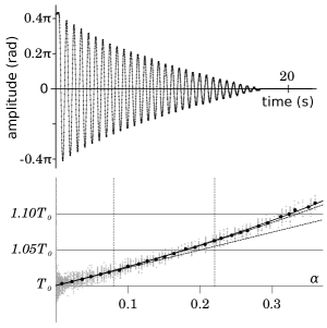
Figure 7: Measuring $K(\alpha)$. Above: Sample amplitude vs. time data. Below: Period vs. energy data points in gray are binned and averaged into the black points. Sequential linear and quadratic fits are depicted as dashed lines, while final cubic fit is a solid line going through all points. Dashed vertical lines mark the boundaries between data subsets.

VI Quantum Classical Analogy

The choice of nomenclature in section III suggests a quantum/classical analogy at work. The symbol $\Psi$ connotes a quantum wavefunction, but above it denotes a C.E.S. Our use of $\Psi$ follows other semi-classical works Harter (1986); Ralston (1989). In the sequel, we extend the analogy to time-independent perturbation theory.

VI.1 Conservation of Energy

Whenever we use approximate methods in the analysis of physical systems, classical or quantum, we also introduce terms of error at some level of precision. For example, approximation of a pendulum’s motion may only conserve total energy up to some power of $\alpha$. A similar situation often arises in quantum mechanics.

We assume a Hamiltonian $H=H_{0}+\epsilon\;V$ for which the eigenstates $|\psi_{n}\rangle$ are approximately known and non-degenerate,

$$H|\psi_{n}\rangle =E_{n}\;|\psi_{n}\rangle$$ (34a)

$$H_{0}|\psi_{n,0}\rangle =E_{n,0}|\psi_{n,0}\rangle.$$ (34b)

The standard perturbation theoryPeebles (1992) determines corrections to the zero-order wavefunctions and energies.

To first order, the time-independent Schrödinger equation becomes

$$H|\psi_{n,1}\rangle=(E_{n,0}+\epsilon\;E_{n,1})|\psi_{n,1}\rangle+\mathcal{O}(\epsilon^{2}).$$ (35)

We make the ansatz

$$|\psi_{n,1}\rangle=|\psi_{n,0}\rangle+\sum_{i\neq n}\epsilon\;c_{n,i}^{1}\;|\psi_{i,0}\rangle,$$ (36)

and solve for

$$c_{n,i}^{1}=\frac{\langle\psi_{i,0}|V|\psi_{n,0}\rangle}{E_{n,0}-E_{i,0}},\;\;\;\;\;E_{n,1}=\langle\psi_{n,0}|V|\psi_{n,0}\rangle.$$ (37)

As with classical perturbation theory, quantum perturbation theory allows iteration to arbitrary $N$ Mathur and Singh (2008), where the approximate eigenfunctions

$$|\psi_{n,N}\rangle=|\psi_{n,0}\rangle+\sum_{j=1}^{N}\sum_{i\neq n}\epsilon^{j}\;c^{j}_{n,i}\;|\psi_{i,0}\rangle,$$ (38)

are nearly stationary with regard to energy

$$H|\psi_{n,N}\rangle=\sum_{i=0}^{N}\epsilon^{i}\;E_{n,i}|\psi_{n,N}\rangle+\mathcal{O}(\epsilon^{N+1}).$$ (39)

Though again a law of diminishing returns applies to higher order corrections.

The semiclassical analogy associates conservation of energy with the eigenvalue equation. In either theory, iteration of a recursive algorithm changes the shape of a C.E.S. or a wavefunction such that the perturbed solution becomes increasingly precise ( Cf. Fig.  8 ).

As time evolves the $N^{th}$ classical approximation satisfies

$$\frac{dE}{dt}=0+\mathcal{O}(\alpha^{N+2}).$$ (40)

To find an analogous equation in quantum dynamics, we apply an infinitesimal time-translation by expanding the Hamiltonian propagator

$$|\psi_{n,N}(t+\Delta t)\rangle=e^{-\frac{i\Delta t}{\hbar}H}|\psi_{n,N}(t)\rangle$$ (41)

$$\approx(1-\frac{i\Delta t}{\hbar}H)|\psi_{n,N}(t)\rangle$$

$$\approx(1-\frac{i\Delta t}{\hbar}\sum_{i=0}^{N}\epsilon^{i}\;E_{n,i})|\psi_{n,N}(t)\rangle+\mathcal{O}(\epsilon^{N+1}).$$

This equation shows that time-evolution acts on the approximate eigenfunctions as a change of complex phase, but only to $\mathcal{O}(\epsilon^{N+1})$. Complex phases cancel in expectation products, so Eq. 41 implies no worse convergence than

$$\frac{d\langle H\rangle}{dt}=0+\mathcal{O}(\epsilon^{N+1}).$$ (42)

As ever, the analogy involves an obvious fallacy: $\alpha$ and $\epsilon$ are dimensionless quantities belonging to two separate classes. In the classical theory, we suppress dependence on the $\epsilon$ coefficients and implicitly assume that a convergence criteria can always be stated as a maximum value for $\alpha$ given an approximation and a precision goal. The quantum theory requires quantization of $\alpha$. After more exploration and explicit calculation, we hope to gain a better understanding of the semiclassical analogy’s inner workings.

VI.2 Quantum Anharmonic Oscillator

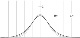
Figure 8: Perturbed oscillator wavefunction. From light gray to black, the approximate wavefunctions for $N=0,1,2$ with parameter values $\epsilon_{1}=-2$ and $h/\lambda_{0}=1$.

We consider the quantum anharmonic oscillator, with Hamiltonian

$$H=\frac{\omega_{0}}{2}(p^{2}+q^{2})+\frac{\omega_{0}}{24}\frac{\epsilon_{1}}{\lambda_{\pi}}\;q^{4}.$$ (43)

Using the technique of ladder operators, it is relatively easy to solve for energy to $\mathcal{O}(\epsilon)$,

$$E_{n,0} =\frac{1}{2}(2n+1)\hbar\omega_{0},$$ (44a)

$$E_{n,1} =\frac{1}{32}(2\;n^{2}+2\;n+1)\hbar\omega_{0},$$ (44b)

where $\hbar=h/(2\pi)$ is the reduced Planck’s constant and $\epsilon=\epsilon_{1}\frac{h}{\lambda_{0}}$.

Setting equal quantum and classical energies, we see that

$$\alpha =\frac{E_{n,0}+\epsilon\;E_{n,1}}{\lambda_{\pi}\;\omega_{0}}+\mathcal{O}(\epsilon^{2})$$

$$=\frac{1}{2}\frac{h}{\lambda_{0}}(2\;n+1)$$

$$+\frac{\epsilon_{1}}{32}(\frac{h}{\lambda_{0}})^{2}(2\;n^{2}+2\;n+1)+\mathcal{O}(\epsilon^{2}),$$

or equivalently, by Eq. 22a,

$$\lambda(n)=(n+\frac{1}{2})h+\frac{\epsilon_{1}}{64}\frac{h^{2}}{\lambda_{0}}+\mathcal{O}(\epsilon^{2}).$$ (46)

The quantum conditions Eqs. 44 & 45 recall the Sommerfeld-Wilson prescription of old quantum mechanicsTomonaga (1968); Child (2014)

$$\lambda(n)=\oint p\;dq=(n+\delta)\;h,$$ (47)

with Maslov index

$$\delta=\frac{1}{2}+\frac{\epsilon_{1}}{64}\frac{h}{\lambda_{0}},$$ (48)

slightly perturbed from $\delta=1/2$, the usual value associated with harmonic vibrational motion.

In the case of a ”quantum pendulum”, $\epsilon_{1}$ can not be made small, so fidelity of approximate methods depends entirely on the constant $\lambda_{0}$. As $l$ and $m$ become increasingly small, $\lambda_{0}$ approaches $h$. Whenever $h/\lambda_{0}<1/10$ and $n<5$ then $\alpha<1/2$, a first or second approximation adequately describes the quantized wavefunctions. The $N=0,1,2$ approximations of the quantum anharmonic oscillator’s groundstate wavefunction appear in Fig.  8, with extreme expansion parameter $h/\lambda_{0}=1$.

VII Conclusion

The pendulum takes an eminent place in the physics canon, not only as a measurement device but also as an example of anharmonic oscillation. The simple harmonic approximation leaves open the possibility of spectacular failure because it only reliably determines the overall scale of time. Apprehension of the dependence on $\theta_{0}$ or $\alpha$ requires more careful and detailed analysis. Here we present a novel algorithm, which solves equations of motion and produces the expansion coefficients of $K(\alpha)$. Calculations require minimal technical skill and avoid any confusing artifice.

Thrift experiment produces good enough data. Taking into account theoretical expectations by writing out a list of prior beliefs, we define an analysis where the extracted parameters closely match the expected values. Nothing precludes our analysis from applying to higher energy motions in the domain $\alpha\in[0,1]$. It would be interesting to see how many expansion coefficients this method may accurately and precisely determine. As many as five, ten?

Perturbation methods extend beyond the important but simple example of a plane pendulum. Extending the ansatz Eq. 19 to include half-powers of $\alpha$ allows arbitrary precision solution of any one-dimensional, power-series potential. This important elaboration leads to applications in mathematical biologyLotka (1920); Arnold and Cooke (1992), classical astronomyKlee (2016d), and relativistic astronomy Klee (2016e). In higher dimensional phase space, we obtain angular equations of motion along a variety of multidimensional C.E.S. Subsequent work will explore the multidimensional generalization.

The classical/quantum analogy reveals fundamental principles that apply throughout physics. Time-independent perturbation theories subject phase space trajectories and wavefunctions to perturbative variations. Evolving through time, trajectories and wavefunctions meet the expectation that higher precision approximations more nearly conserve energy. Exploration of quantum conditions resolves a fallacy in the analogy by showing that quantum theory replaces continuous energy parameter $\alpha$ with a quantum number $n$. We have yet to find any connections to the Matheiu functionsLeibscher and Schmidt (2009), but speculate of their existence.

Ultimately we reach a detailed understanding of the plane pendulum and its relation to time. The pendulum is a particular anharmonic oscillator, with a period that varies slightly as a function of amplitude. On the quantum scale atomic oscillations, for example in Cesium-133, provide the highest precision time scales. On the astronomical scale, we also measure long times, even for the practical purpose of keeping a calendar. Seconds are useful units for time, but physics also needs nanoseconds and years. Wherever we find an oscillation, usually anharmonicity is not too far behind, leading to unexpected behaviors such as precession.

References

- Ariotti [1968] P. Ariotti. Galileo on the isochrony of the pendulum. Isis, 59(4):414–426, 1968.
- Landau and Lifshitz [1976] L.D. Landau and E.M. Lifshitz. Mechanics. Pergamon Press, 1976.
- Harter [2016] W.G. Harter. Classical mechanics with a BANG!, 2016. URL https://goo.gl/CCN11y.
- Jacobi [1829] C. G. J. Jacobi. Fundamenta Nova Theoriae Functionum Ellipticarum. Königsberg, 1829.
- Brizard [2009] A.J. Brizard. A primer on elliptic functions with applications in classical mechanics. European Journal of Physics, 30(4):729, 2009.
- Baker and Bill [2012] T.E. Baker and A. Bill. Jacobi elliptic functions and the complete solution to the bead on the hoop problem. American Journal of Physics, 80(6):506–514, 2012.
- Erdös [2000] P. Erdös. Spiraling the earth with C.G.J. Jacobi. American Journal of Physics, 68(10):888–895, 2000.
- Carvalhaes and Suppes [2008] C.G. Carvalhaes and P. Suppes. Approximations for the period of the simple pendulum based on the arithmetic-geometric mean. American Journal of Physics, 76(12):1150–1154, 2008.
- Kidd and Fogg [2002] R.B. Kidd and S.L. Fogg. A simple formula for the large-angle pendulum period. The Physics Teacher, 40(2):81–83, 2002.
- Fulcher and Davis [1976] L.P. Fulcher and B.F. Davis. Theoretical and experimental study of the motion of the simple pendulum. American Journal of Physics, 44(1):51–55, 1976.
- Park [2012] D. Park. Classical Dynamics and Its Quantum Analogues. Springer, 2012.
- Lowenstein [2012] J.H. Lowenstein. Essentials of Hamiltonian Dynamics. Cambridge University Press, 2012.
- Research [2016] Wolfram Research. Wolfram functions: Elliptic functions, 2016. URL https://goo.gl/bzBNqj.
- Nelson and Olsson [1986] R.A. Nelson and M.G. Olsson. The pendulum-rich physics from a simple system. American Journal of Physics, 54(2):112–121, 1986.
- Ralston [1989] J.P. Ralston. Berry’s phase and the symplectic character of quantum time evolution. Physical Review A, 40(9):4872, 1989.
- Arnold [2013] V.I. Arnold. Mathematical Methods of Classical Mechanics. Graduate Texts in Mathematics. Springer New York, 2013.
- Collaboration [2016] The OEIS Collaboration. The on-line encyclopedia of integer sequences, 2016. URL http://oeis.org.
- Klee [2016a] B. Klee. Approximating the jacobian elliptic functions, 2016a. URL https://goo.gl/o7Cg7x.
- Lang [2016] W. Lang. Private communication, 2016.
- Whittaker and Watson [1927] E.T. Whittaker and G.N. Watson. Modern analysis. Cambridge University Press, 1927.
- Forest and Ruth [1990] E. Forest and R.D. Ruth. Fourth-order symplectic integration. Physica D: Nonlinear Phenomena, 43(1):105–117, 1990.
- Abramowitz and Stegun [1964] M. Abramowitz and I.A. Stegun. Handbook of mathematical functions, volume 55. Courier Corporation, 1964.
- Stein [2016] L.C. Stein. Private communication, 2016.
- Seiffert [1896] A. Seiffert. Über eine neue geometrische Einführung in die Theorie der elliptischen Funktionen. Wissenschaftliche Beilage zum Jahresbericht der Städtischen Realschule zu Charlottenburg, Ostern, 1896.
- Gintautas and Hübler [2009] V. Gintautas and A. Hübler. A simple, low-cost, data-logging pendulum built from a computer mouse. Physics Education, 44(5):488, 2009.
- Peters and Lee [2009] R.D. Peters and S.C. Lee. Pendulum sensor using an optical mouse. arXiv:0904.3070, 2009.
- [27] Arch Linux Collaboration. Xorg - ArchWiki. URL https://wiki.archlinux.org/index.php/xorg.
- Lewowski and Wozniak [2002] T. Lewowski and K. Wozniak. The period of a pendulum at large amplitudes: a laboratory experiment. European journal of physics, 23(5):461, 2002.
- Nicklin and Rafert [1984] R.C. Nicklin and J.B. Rafert. The digital pendulum. American Journal of Physics, 52(7):632–639, 1984.
- S. Gil and Gregorio [2008] A.E. Legarreta S. Gil and D.E. Di Gregorio. Measuring anharmonicity in a large amplitude pendulum. American Journal of Physics, 76(9):843–847, 2008.
- Klee [2016b] B. Klee. Github - digital pendulum data analysis, 2016b. URL https://goo.gl/juvySd.
- Klee [2016c] B. Klee. AUR(en) - pendulumdata, 2016c. URL https://goo.gl/m1JEMQ.
- Harter [1986] W.G. Harter. Su(2) coordinate geometry for semiclassical theory of rotors and oscillators. The Journal of chemical physics, 85(10):5560–5574, 1986.
- Peebles [1992] P.J.E. Peebles. Quantum Mechanics. Princeton University Press, 1992.
- Mathur and Singh [2008] V.S. Mathur and S. Singh. Concepts in quantum mechanics. CRC Press, 2008.
- Tomonaga [1968] S. Tomonaga. Quantum Mechanics: I, Old quantum theory. North-Holland, 1968.
- Child [2014] M.S. Child. Semiclassical mechanics with molecular applications. Clarendon Press, Oxford, 2014.
- Lotka [1920] A.J. Lotka. Analytical note on certain rhythmic relations in organic systems. Proceedings of the National Academy of Sciences, 6(7):410–415, 1920.
- Arnold and Cooke [1992] V.I. Arnold and R. Cooke. Ordinary Differential Equations. Springer Textbook. Springer Berlin Heidelberg, 1992. ISBN 9783540548133.
- Klee [2016d] B. Klee. Estimating planetary perihelion precession, 2016d. URL https://goo.gl/wCrwx0.
- Klee [2016e] B. Klee. Exact and approximate relativistic corrections to the orbital precession of mercury, 2016e. URL https://goo.gl/Y2k7yX.
- Leibscher and Schmidt [2009] M. Leibscher and B. Schmidt. Quantum dynamics of a plane pendulum. Physical Review A, 80(1):012510, 2009.