Mixed Marginal Copula Modeling

Abstract

This article extends the literature on copulas with discrete or continuous marginals to the case where some of the marginals are a mixture of discrete and continuous components. We do so by carefully defining the likelihood as the density of the observations with respect to a mixed measure. The treatment is quite general, although we focus focus on mixtures of Gaussian and Archimedean copulas. The inference is Bayesian with the estimation carried out by Markov chain Monte Carlo. We illustrate the methodology and algorithms by applying them to estimate a multivariate income dynamics model.

Keywords: Bayesian analysis; Markov chain Monte Carlo; Mixtures of copulas; Multivariate income dynamics.

1 Introduction

Copulas are a versatile and useful tool for modeling multivariate distributions. See, for example, Fan and Patton (2014), Patton (2009), Durante and Sempi (2015) and Trivedi and Zimmer (2007). Modeling non-continuous marginal random variables is a challenging task due to computational problems, interpretation difficulties and various other pitfalls and paradoxes; see Smith and Khaled (2012), for example. The main source of the computational issues arises from the difficulty of directly evaluating the likelihood. For example, when modeling a vector of $m$ discrete random variables, evaluating the likelihood at one point requires computing $2^{m}$ terms. The literature on modeling non-continuous random marginal problems has mostly focused on cases where all the marginals are discrete, and less extensively, on cases where some marginals are discrete and some are continuous. See, for example, Genest and Neslehová (2007), Smith and Khaled (2012), De Leon and Chough (2013), and Panagiotelis et al. (2012). Furthermore, a lot of the literature has focused on approaches restricted to certain classes to copulas. For example, this is the case for Gaussian copulas (See for instance Shen and Weissfeld (2006), Hoff (2007), Song et al. (2009), de Leon and Wu (2011), He et al. (2012) and Jiryaie et al. (2016)) or pair-copula constructions (see Stöber et al. (2015)). Relatively little attention has been paid to the case where some variables are a mixture of discrete and continuous components. In contrast, our approach, presents methodology for an arbitrary copula and can be applied quite generally as long as it is possible to compute certain marginal and conditional copulas either in closed-form or numerically.

Our article extends the Bayesian methodology used for estimating continuous marginals to the case where each marginal can be a mixture of an absolutely continuous random variable and a discrete random variable. In particular, we are interested in applying the new methodology to copulas that are mixtures of Gaussian and Archimedean copulas. To illustrate the methodology and sampling algorithm we apply them to estimate a multivariate income dynamics model. In this application, we use the copula framework to model the dependence structure of random variables that are mixtures of discrete and continuous components, and apply the model to empirical economic data. We note that there are many other real world economic applications that involve such mixtures of random variables as marginals, and these are briefly discussed in Section 5.

Our proposed methodology extends that introduced in Pitt et al. (2006) and Smith and Khaled (2012). Smith and Khaled (2012) allow the joint modeling of distributions of random variables such that each component can be either discrete or continuous. However, neither paper covers the case where some random variables can be a mixture of an absolutely continuous random variable and a discrete random variable. In a financial econometrics application, Brechmann et al. (2014) consider the case where the marginal distributions are mixtures of continuous and points of probability mass at zero. In contrast, our paper derives the likelihood equations in a much more general setting that allows for the margins to be arbitrarily classified into three groups: absolutely continuous, discrete and mixtures of absolutely continuous and discrete random variables. Furthermore, there is no restriction on the number or location of the point masses present in each margin. This can occur in many economic data, for instance in cases where earnings are top-coded and have individuals with zero earnings. Equally, our setting covers the case of dependent interval-censored data.

The paper is organized as follows. Section 2 outlines the copula model and defines the likelihood as a density with respect to a mixed measure. Section 3 presents the simulation algorithms used for inference. Section 4 applies the methods and algorithms to model multivariate income dynamics. This section describes the data and presents the estimation results. Section 5 concludes. The paper has two appendices. Appendix A defines the difference notation which is a handy tool useful when writing formulas for the likelihood of our model in closed-form. Appendix B presents and proves the results required to define the likelihood as a density with respect to a mixed measure. The paper also has an online supplement whose sections are denoted as Sections S1, etc. Section S1 describes the Gaussian and Archimedean copulas used in the article, as well as the Markov chain Monte Carlo (MCMC) sampling scheme. Section S2 introduces a new three dimensional example to further illustrate the methods in the paper. Section S3 gives a proof of Lemma 3 which is discussed in Appendix B. Section S4 presents some additional empirical results.

2 Defining the Likelihood of a general copula

This section discusses the proposed model and shows how to write the likelihood of an i.i.d. sample from it. Each random vector is modeled using a marginal distribution-copula decomposition and each marginal is allowed to be a mixture of an absolutely continuous component and a discrete component. The MCMC sampling scheme in the next section is based on this definition of the likelihood.

Let $\bm{X}=(X_{1},\ldots,X_{m})$ be an $\text{R}^{m}$-valued random vector. If, for example, $X_{j}$ is categorical, then its support would be a finite subset of R and thus without loss of generality, we can work with $\text{R}^{m}$. Let $\mathcal{M}=\{1,\ldots,m\}$ be the index set, and $2^{\mathcal{M}}$ its power-set (or the set of all of its subsets). Let the random variable $X_{j}$ have cumulative distribution function $F_{j}$ for $j=1,\ldots,m$. By the Lebesgue decomposition theorem (Shorack, 2000, Chapter 7, Theorem 1.1), and assuming there are no continuous singularities (see Durante and Sempi, 2015, for a detailed discussion), the distribution of each $X_{j}$ can be written as a mixture of an absolutely continuous random variable and a discrete random variable. This means that $F_{j}$ is allowed to have jumps at a countable number of points. In order to exploit this result, we would like to be able to decide at each point of $\text{R}^{m}$, which indices have jumps in their corresponding CDFs.

We need a mapping $\mathcal{C}:\text{R}^{m}\rightarrow 2^{\mathcal{M}}$ that, for each $\bm{x}\in\text{R}^{m}$, picks out the subset of the indices of $\bm{x}$ where $F_{j}$ is continuous at $x_{j}$ for each $j\in\mathcal{C}(\bm{x})$.

$$\mathcal{C}:\text{R}^{m} \longrightarrow 2^{\mathcal{M}}\quad\text{with}\quad\bm{x}\longrightarrow\mathcal{C}(\bm{x}).$$

Similarly, we define the set $\mathcal{D}(\bm{x})=\mathcal{M}-\mathcal{C}(\bm{x})$ (the complement of $\mathcal{C}(\bm{x})$ in $\mathcal{M}$, that is the set of indices $j$ for which $F_{j}$ presents jumps at $x_{j}$). This means that for all $\bm{x}\in\text{R}^{m}$, $\{\mathcal{C}(\bm{x}),\mathcal{D}(\bm{x})\}$ partitions the index set so that $\mathcal{C}(\bm{x})\cap\mathcal{D}(\bm{x})=\varnothing$ and $\mathcal{C}(\bm{x})\cup\mathcal{D}(\bm{x})=\mathcal{M}$.

As a first example, consider $\bm{X}=(X_{1},X_{2})$, where $X_{1}\sim\mathcal{N}(0,1)$ and $X_{2}$ is a mixture of an exponential distribution with parameter $\lambda$ and a point mass at $0$ with probability $p$, i.e., $X_{2}\sim p\delta_{0}+(1-p)\mathcal{E}(\lambda)$). Then, $\mathcal{C}(x_{1},0)=\{1\}$ for all $x_{1}\in\text{R}$ and $\mathcal{C}(x_{1},x_{2})=\{1,2\}$ for all $x_{1}\in\text{R},x_{2}\char 62\relax 0$. Similarly $\mathcal{D}(x_{1},0)=\{2\}$ for all $x_{1}\in\text{R}$ and $\mathcal{D}(x_{1},x_{2})=\varnothing$.

As a second example, let $\bm{X}=(X_{1},X_{2})$, where $X_{1}$ is Bernoulli and $X_{2}\sim\mathcal{N}(0,1)$. Then $\mathcal{C}(\bm{x})=\{2\}$ for all $\bm{x}\in\{0,1\}\times\text{R}$. Similarly $\mathcal{D}(\bm{x})=\{1\}$ for all $\bm{x}$.

Let $\bm{U}=(U_{1},\ldots,U_{m})$ be a vector of uniform random variables whose distribution is given by some copula $C$. We assume that $F_{j}^{-1}$ is the quantile function corresponding to $F_{j}$ (since $F_{j}$ is not invertible when $X_{j}$ is not absolutely continuous, this corresponds to picking one possible generalized inverse function).

The variables $\bm{U}$ are selected to satisfy the following criteria. If, at coordinate $x_{j}$, $j\in\mathcal{C}(\bm{x})$, then $u_{j}=F_{j}(x_{j})$, resulting in a deterministic one-to-one relationship when conditioning on either $U_{j}$ or $X_{j}$. Otherwise, $j\in\mathcal{D}(\bm{x})$, and we require $x_{j}=F_{j}^{-1}(u_{j})$, resulting in an infinity of $U_{j}$ corresponding to one $X_{j}$ and spanning the interval $(F_{j}(X_{j}^{-}),F_{j}(X_{j}))$. This interval corresponds to gaps in the range of $F_{j}$. If $\mathcal{C}(\bm{x})=\mathcal{M}$ for every $\bm{x}$, then $C$ will be the copula of $\bm{X}$. Otherwise, the copula structure will still create dependence between the non-continuous marginal variables but will not be unique in general. Mathematically, the above description leads to the joint density

$$f(\bm{x},\bm{u}):=c(\bm{u})\prod_{j\in\mathcal{C}(\bm{x})}\mathcal{I}(u_{j}=F_{j}(x_{j}))\prod_{j^{\prime}\in\mathcal{D}(\bm{x})}\mathcal{I}(F_{j^{\prime}}(x_{j^{\prime}}^{-})\leqslant u_{j^{\prime}}\char 60\relax F_{j^{\prime}}(x_{j^{\prime}})),$$ (1)

where $c$ is the copula density corresponding to $C$ and $\mathcal{I}$ is an indicator variable. See Lemma 4, part (i), of Appendix  B for a derivation of (1) and the corresponding measure. Notice that in  (1), products over the indices $j$ and $j^{\prime}$ correspond to different partitions for each $\bm{x}$.

With a small abuse of notation, we call $\bm{U}$ the vector of latent variables, even though $U_{j}$ is a deterministic function of $X_{j}$ if $F_{j}$ is invertible.

To derive the likelihood function, that is the marginal density of $\bm{X}$, from the joint density $f(\bm{x},\bm{u})$, we introduce some notation. Let $\bm{a},\bm{b}$ be two vectors in $\text{R}^{k}$ such that $\bm{a}\leqslant\bm{b}$ componentwise and let $g$ be an arbitrary function from $\text{R}^{k}$ into R. We denote by $\bigtriangleup_{\bm{a}}^{\bm{b}}g(.)$ the sum of $2^{k}$ terms that are obtained by repeatedly subtracting $g(.,a_{j},.)$ from $g(.,b_{j},.)$ for each $j=1,\ldots,k$. Appendix A contains more details on using this notation.

For each $\bm{x}\in\text{R}^{m}$, denote by $\bm{b}=(F_{1}(x_{1}),\ldots,F_{m}(x_{m}))$ the vector of upper bounds and similarly denote by $\bm{a}=(F_{1}(x_{1}^{-}),\ldots,F_{m}(x_{m}^{-}))$ the vector of lower bounds. For each $j\in\mathcal{C}(\bm{x})$, $\bm{b}(j)=\bm{a}(j)$, otherwise we have the strict inequality $\bm{b}(j)\char 62\relax\bm{a}(j)$. Denote the partitions of $\bm{a}$ and $\bm{b}$ by $\bm{a}_{\mathcal{C}(\bm{x})}$, $\bm{a}_{\mathcal{D}(\bm{x})}$, $\bm{b}_{\mathcal{C}(\bm{x})}$ and $\bm{b}_{\mathcal{D}(\bm{x})}$. For some sets $A,B\subset\mathcal{M}$, denote by $c_{A}$ and $c_{A|B}$,  the marginal copula density over the indices of $A$, the conditional copula density where the variables in $A$ are conditioned on the variables with index set $B$. It is possible to do the same for $C_{A}$ and $C_{A|B}$, the copula distribution functions.

If $(\bm{X},\bm{U})$ has the joint density given by (1), then the marginal density of $\bm{X}$ is

$$f(\bm{x})=c_{\mathcal{C}(\bm{x})}(\bm{b}_{\mathcal{C}(\bm{x})})\prod_{j\in\mathcal{C}(\bm{x})}f_{j}(x_{j})\bigtriangleup_{\bm{a}_{\mathcal{D}(\bm{x})}}^{\bm{b}_{\mathcal{D}(\bm{x})}}C_{\mathcal{D}(\bm{x})|\mathcal{C}(\bm{x})}(\cdot|\bm{b}_{\mathcal{C}(\bm{x})}),$$ (2)

which corresponds to writing the formula for the density of $\bm{X}$ as the product of the (marginal) density of continuous components at $\bm{x}$

$$f(\bm{x}_{\mathcal{C}(\bm{x})})=c_{\mathcal{C}(\bm{x})}(\bm{b}_{\mathcal{C}(\bm{x})})\prod_{j\in\mathcal{C}(\bm{x})}f_{j}(x_{j}),$$

and the (conditional) density of the non-continuous components conditional on the continuous ones

$$f(\bm{x}_{\mathcal{D}(\bm{x})}|\bm{x}_{\mathcal{C}(\bm{x})})=\bigtriangleup_{\bm{a}_{\mathcal{D}(\bm{x})}}^{\bm{b}_{\mathcal{D}(\bm{x})}}C_{\mathcal{D}(\bm{x})|\mathcal{C}(\bm{x})}(\cdot|\bm{b}_{\mathcal{C}(\bm{x})}).$$

See Lemma 4, part (ii), of Appendix  B for a derivation of (2) and the corresponding measure.

We now give a bivariate example to illustrate how the formulas can be used. This example is continued in later sections. See also Section S2 for a trivariate illustrative example.

Example 1 (running illustrative example).

Let $X_{1}$ have a density that is a mixture of point of probability mass at zero and a normal distribution $f_{1}(x_{1})\sim\pi\delta_{x_{1}}(0)+(1-\pi)\phi(x_{1})$ where $\phi(.)$ is the density of a standard normal. This implies that the cumulative distribution function of $X_{1}$ is

$$F_{1}(x_{1})=(1-\pi)\Phi(x_{1})+\pi\mathcal{I}(x_{1}\geqslant 0),$$

and thus there a discontinuity in $F_{1}$ at the point 0. Let $X_{2}$ be a binary random variable with $\Pr\{X_{2}=0\}=\gamma$.

Let $C(\cdot)$ and $c(\cdot)$ be respectively the Clayton copula and Clayton copula density with parameter $\theta=1$, so that

$$C(u_{1},u_{2})=\left(\frac{1}{u_{1}}+\frac{1}{u_{2}}-1\right)^{-1},\quad c(u_{1},u_{2})=\frac{2}{u_{1}^{2}u_{2}^{2}}\left(\frac{1}{u_{1}}+\frac{1}{u_{2}}-1\right)^{-3}$$

and the conditional copula is given by

$$C_{2|1}(u_{2}|u_{1})=\frac{1}{u_{1}^{2}}\left(\frac{1}{u_{1}}+\frac{1}{u_{2}}-1\right)^{-2},$$

which has the conditional quantile function $C^{-1}(\tau|u_{1})=\frac{\sqrt{\tau}u_{1}}{1+\sqrt{\tau}(u_{1}-1)}$ and the conditional density $c_{2|1}(u_{2}|u_{1})=c(u_{1},u_{2})$ (because the marginal of $u_{1}$ is uniform).

The following details are necessary construct the example.

$\mathcal{C}(\bm{x})=\{2\}$ for $x_{1}\neq 0$, for all $x_{2}$ and $\mathcal{C}(\bm{x})=\{1,2\}$ for $x_{1}=0$, for all $x_{2}$

Joint of $\bm{x}$ and $\bm{u}$ ( Eq. (1) )

There are two cases. Case 1: $x_{1}\neq 0$

$f(x_{1},x_{2},u_{1},u_{2})=c(u_{1},u_{2})\mathcal{I}(u_{1}=F_{1}(x_{1}))\mathcal{I}(F_{2}(x_{2}-)\leqslant u_{2}\char 60\relax F_{2}(x_{2}))$

Case 2: $x_{1}=0$

$f(x_{1},x_{2},u_{1},u_{2})=c(u_{1},u_{2})\mathcal{I}(F_{1}(0-)\leqslant u_{1}\char 60\relax F_{1}(0))\mathcal{I}(F_{2}(x_{2}-)\leqslant u_{2}\char 60\relax F_{2}(x_{2}))$

Likelihood at one point (Eq. 2 )

If $x_{1}\neq 0$, then

$$f(x_{1},x_{2}) = f(x_{1})\bigtriangleup_{F_{2}(x_{2}-)}^{F_{2}(x_{2})}C_{2|1}(\cdot|F(x_{1}))$$

$$= f_{1}(x_{1})\{C_{2|1}(F_{2}(x_{2})|F_{1}(x_{1}))-C_{2|1}(F_{2}(x_{2}-)|F_{1}(x_{1}))\}$$

because $c(u_{1})=1$ as one-dimensional margins of a copula are all uniform. If $x_{1}=0$, then

$$f(0,x_{2}) = \bigtriangleup_{F_{1}(0-)}^{F_{1}(0)}\bigtriangleup_{F_{2}(x_{2}-)}^{F_{2}(x_{2})}C(\cdot)$$

$$= \bigtriangleup_{F_{1}(0-)}^{F_{1}(0)}\{C(\cdot,F_{2}(x_{2}))-C(\cdot,F_{2}(x_{2}-))\}$$

$$= C(F_{1}(0),F_{2}(x_{2}))-C(F_{1}(0),F_{2}(x_{2}-))-C(F_{1}(0-),F_{2}(x_{2}))+C(F_{1}(0-),F_{2}(x_{2}-)).$$

The difficult part of implementing a simulation algorithm based on equations (1) and (2) is that the size of the vectors $\bm{x}_{\mathcal{C}(\bm{x})}$ and $\bm{x}_{\mathcal{D}(\bm{x})}$ changes with $\bm{x}$. A secondary difficulty is that the second term is a sum of $2^{|\mathcal{D}(\bm{x})|}$ terms for each $\bm{x}$, where $|\mathcal{D}(\bm{x})|$ is the cardinality of the set $\mathcal{D}(\bm{x})$.

3 Estimation and Algorithms

3.1 Conditional distribution of the latent variables

In any simulation scheme (such as MCMC or simulated EM) where the latent variables $\bm{U}$ are used to carry out inference, it is necessary to know the distribution of $\bm{U}|\bm{X}$. This distribution is singular due to the deterministic relationship over $\mathcal{C}(\bm{x})$ for each $\bm{x}\in\text{R}^{m}$. For this reason, it is useful to work only with $\bm{U}_{\mathcal{D}(\bm{x})}|\bm{X}$. A second issue is the need to work with different sizes of vectors $\bm{U}_{\mathcal{D}(\bm{x})}$ for each $\bm{x}$ in our sample (say $\bm{x}_{1},\ldots,\bm{x}_{n}$), so we will be working with $n$ distributions over different spaces. Recursively using Bayes formula and similar integration arguments to the ones described during the derivation of the $\bm{X}$ density, we obtain the density for $\bm{U}_{\mathcal{D}(\bm{x})}|\bm{X}$ as

$$f(\bm{u}_{\mathcal{D}(\bm{x})}|\bm{x})=\frac{c_{\mathcal{D}(\bm{x})|\mathcal{C}(\bm{x})}(\bm{u}_{\mathcal{D}(\bm{x})}|\bm{b}_{\mathcal{C}(\bm{x})})\prod_{j\in\mathcal{D}(\bm{x})}\mathcal{I}(a_{j}\leqslant u_{j}\char 60\relax b_{j})}{\bigtriangleup_{\bm{a}_{\mathcal{D}(\bm{x})}}^{\bm{b}_{\mathcal{D}(\bm{x})}}C_{\mathcal{D}(\bm{x})|\mathcal{C}(\bm{x})}(\cdot|\bm{b}_{\mathcal{C}(\bm{x})})},$$ (3)

where the denominator is a constant of integration. As seen from the above conditional density, one of the complexities arising is that the distribution $\bm{U}_{\mathcal{D}(\bm{x})}|\bm{X}=\bm{x}$ depends on the whole vector $\bm{x}$ and not just on $\bm{x}_{\mathcal{D}(\bm{x})}$. See Lemma 4, part (iii), of Appendix  B for a derivation of (3) and the corresponding measure.

We can now proceed in two ways. We can either draw each $U_{j}$ in $\bm{U}_{\mathcal{D}(\bm{x})}$ separately conditionally on everything else. This is reminiscent of a single move Gibbs sampler. Alternatively, it turns out that in spite of the difficulties, the above distribution can also be sampled recursively without having to compute any of the above normalizing constants. By writing $\mathcal{D}(\bm{x})$ as $\{j_{1},\ldots,j_{|\mathcal{D}(\bm{x})|}\}$, we can use the following scheme

• $U_{j_{1}}|\bm{X}$

• $U_{j_{2}}|U_{j_{1}},\bm{X}$

• $\vdots$

• $U_{j_{|\mathcal{D}(\bm{x})|}}|U_{j_{1}},\ldots,U_{j_{|\mathcal{D}(\bm{x})|-1}},\bm{X}$

We now note that the order of the indices $j_{1},...,j_{|\mathcal{D}(\bm{x})|}$ is irrelevant for the sampling scheme. Although it might appear that the sampling procedure depends on the ordering of those indices, the acceptance or rejection of such samples also depends on the ordering and the next subsection shows that such a procedure will always result in a correct MCMC draw from the conditional distribution $\bm{U}_{\mathcal{D}(\bm{x})}|\bm{X}$.

The above sampling scheme requires knowing the marginal distribution of $\bm{U}_{\mathcal{J}}|\bm{X}$ for $\mathcal{J}\subset\mathcal{D}(\bm{x})$ and the conditional decomposition $U_{j}|\bm{U}_{\mathcal{K}},\bm{X}$ where $(\{j\},\mathcal{K})$ is a partition of $\mathcal{J}$ (meaning $\{j\}=\mathcal{J}\backslash\mathcal{K}$, the complement of $\mathcal{K}$ in $\mathcal{J}$). This distribution can be derived as

$$f(\bm{u}_{\mathcal{J}}|\bm{x}) = \frac{c(\bm{b}_{\mathcal{C}(\bm{x})})\prod_{j\in\mathcal{C}(\bm{x})}f(x_{j})}{f(\bm{x})}c(\bm{u}_{\mathcal{J}}|\bm{b}_{\mathcal{C}(\bm{x})})$$

$$\times \left[\bigtriangleup_{\bm{a}_{\mathcal{J}^{c}}}^{\bm{b}_{\mathcal{J}^{c}}}C_{\bm{U}_{\mathcal{J}^{c}}|\bm{U}_{\mathcal{J}},\bm{U}_{\mathcal{C}(\bm{x})}}(\cdot|\bm{u}_{\mathcal{J}},\bm{b}_{\mathcal{C}(\bm{x})})\right]\prod_{j\in\mathcal{J}}\mathcal{I}(a_{j}\leqslant u_{j}\char 60\relax b_{j})$$

with $\mathcal{J}^{c}=\mathcal{D}(\bm{x})\backslash\mathcal{J}$ and

$$f(u_{j}|\bm{u}_{\mathcal{K}},\bm{x}) = c(u_{j}|\bm{u}_{\mathcal{K}},\bm{b}_{\mathcal{C}(\bm{x})})\mathcal{I}(a_{j}\leqslant u_{j}\char 60\relax b_{j})$$

$$\times \frac{\bigtriangleup_{\bm{a}_{\mathcal{J}^{c}}}^{\bm{b}_{\mathcal{J}^{c}}}C_{\bm{U}_{\mathcal{J}^{c}}|\bm{U}_{\mathcal{J}},\bm{U}_{\mathcal{C}}}(\cdot|\bm{u}_{\mathcal{J}},\bm{b}_{\mathcal{C}(\bm{x})})}{\bigtriangleup_{\bm{a}_{\mathcal{K}^{c}}}^{\bm{b}_{\mathcal{K}^{c}}}C_{\bm{U}_{\mathcal{K}^{c}}|\bm{U}_{\mathcal{K}},\bm{U}_{\mathcal{C}}}(\cdot|\bm{u}_{\mathcal{K}},\bm{b}_{\mathcal{C}(\bm{x})})},$$

where $\mathcal{K}^{c}=\mathcal{J}^{c}\cup\{j\}$.

We continue to illustrate how to apply the latent variables conditional formulas by considering Example 1.

Example 1 (continued).

If $x_{1}\neq 0$, then

$$f(u_{2}|\bm{x})=\frac{c_{2|1}(u_{2}|F_{1}(x_{1}))\mathcal{I}(F_{2}(x_{2}-)\leqslant u_{2}\char 60\relax F_{2}(x_{2}))}{C_{2|1}(F_{2}(x_{2})|F_{1}(x_{1}))-C_{2|1}(F_{2}(x_{2}-)|F_{1}(x_{1}))}$$

($u_{1}$ is deterministically equal to $F_{1}(x_{1})$, so we only need to sample $u_{2}$).

If $x_{1}=0$

$$f(u_{1},u_{2}|\bm{x})=\frac{c(u_{1},u_{2})\mathcal{I}(F_{1}(0-)\leqslant u_{1}\char 60\relax F_{1}(0))\mathcal{I}(F_{2}(x_{2}-)\leqslant u_{2}\char 60\relax F_{2}(x_{2}))}{C(F_{1}(0),F_{2}(x_{2}))-C(F_{1}(0),F_{2}(x_{2}-))-C(F_{1}(0-),F_{2}(x_{2}))+C(F_{1}(0-),F_{2}(x_{2}-))}$$

3.2 Metropolis-Hastings sampling

It is clear from the formulas for $f(u_{j}|\bm{u}_{\mathcal{K}},\bm{x})$ that they are quite intricate. They correspond to a product of a simple term $c(u_{j}|\bm{u}_{\mathcal{K}},\bm{b}_{\mathcal{C}(\bm{x})})\mathcal{I}(a_{j}\leqslant u_{j}\char 60\relax b_{j})$ (a truncated conditional copula density) and a complicated term that depends on ratios of normalizing constants for $f(\bm{u}_{\mathcal{J}}|\bm{x})$ and $f(\bm{u}_{\mathcal{K}}|\bm{x})$. One of the most useful aspects of the Metropolis-Hastings (MH) algorithm is that it does not require knowledge of normalizing constants. The trick here is that those normalizing constants are obtained recursively. Assume that we sample

• $U_{j_{1}}$ from $c(u_{j_{1}})\mathcal{I}(a_{j_{1}}\leqslant u_{j_{1}}\char 60\relax b_{j_{1}})$

• $U_{j_{2}}$ from $c(u_{j_{2}}|u_{j_{1}})\mathcal{I}(a_{j_{2}}\leqslant u_{j_{2}}\char 60\relax b_{j_{2}})$

• $\vdots$

• $U_{j_{|\mathcal{D}(\bm{x})|}}$ from $c(u_{j_{|\mathcal{D}(\bm{x})|}}|u_{j_{1}},\ldots,u_{j_{|\mathcal{D}(\bm{x})|-1}})\mathcal{I}(a_{j_{|\mathcal{D}(\bm{x})|}}\leqslant u_{j_{|\mathcal{D}(\bm{x})|}}\char 60\relax b_{j_{|\mathcal{D}(\bm{x})|}})$

that is, if we use as proposal a truncated form of the copula marginal density over $\mathcal{D}(\bm{x})$, then computing the MH accept/reject ratio results in the computationally simple formula

$$\alpha(\bm{x}_{i})=\prod_{k=1}^{|\mathcal{D}(\bm{x})|}\frac{C(F_{j_{k}}(x_{i,j_{k}})|u^{N}_{i,j_{1}},\ldots,u^{N}_{i,j_{k-1}},\bm{b}_{\mathcal{C}(\bm{x}_{i}),i})-C(F_{j_{k}}(x_{i,j_{k}}^{-})|u^{N}_{i,j_{1}},\ldots,u^{N}_{i,j_{k-1}},\bm{b}_{\mathcal{C}(\bm{x}_{i}),i})}{C(F_{j_{k}}(x_{i,j_{k}})|u^{O}_{i,j_{1}},\ldots,u^{O}_{i,j_{k-1}},\bm{b}_{\mathcal{C}(\bm{x}_{i}),i})-C(F_{j_{k}}(x_{i,j_{k}}^{-})|u^{O}_{i,j_{1}},\ldots,u^{O}_{i,j_{k-1}},\bm{b}_{\mathcal{C}(\bm{x}_{i}),i})}$$

where $i$ represents the observation index. The complexity of this formula is much smaller than $2^{|\mathcal{D}(\bm{x})|}$.

We now illustrate the Metropolis-Hastings acceptance probabilities by again considering Example 1.

Example 1 (continued).

If $x_{1}\neq 0$, then the ratio is $\alpha(x_{2})=1$ and if $x_{1}=0$ (first draw $u_{1}^{N}$ from a uniform on $(F_{1}(0^{-}),F_{1}(0))$ and compare to the previous draw $u_{1}^{O}$)

$$\alpha(0,x_{2})=\frac{C_{2|1}(F_{2}(x_{2})|u_{1}^{N})-C_{2|1}(F_{2}(x_{2}^{-})|u_{1}^{N})}{C_{2|1}(F_{2}(x_{2})|u_{1}^{O})-C_{2|1}(F_{2}(x_{2}^{-})|u_{1}^{O})}$$

Note that here the ordering does not matter, as we could have computed the other ratio (if we draw instead first $u_{2}^{N}$ from a uniform on $(F_{2}(x_{2}^{-}),F_{2}(x_{2}))$

$$\alpha(0,x_{2})=\frac{C_{1|2}(F_{1}(0)|u_{2}^{N})-C_{1|2}(F_{1}(0^{-})|u_{2}^{N})}{C_{1|2}(F_{1}(0)|u_{2}^{O})-C_{1|2}(F_{1}(0^{-})|u_{2}^{O})}$$

Even though the ratio are different, both procedures will result in a draw from $f(u_{1},u_{2}|\bm{x})$.

3.3 Mixtures of Archimedean and Gaussian copulas

This section applies the previous results to the family of mixtures of Archimedean and Gaussian copulas. Working with mixtures of copulas provides a simple and yet rich and flexible modeling framework because mixtures of copulas are copulas themselves,

We are particularly interested in having a mixture of three components, two Archimedean copulas, the Clayton copula $\left(C_{Cl}\right)$ and the Gumbel copula $\left(c_{Gu}\right)$ and a Gaussian copula $\left(c_{G}\right)$ component. We will later apply this mixture to model the dependence between individual income distributions over 13 years. The copula density of this 3-component mixture is

$$c_{mix}\left(\bm{u};\Gamma,\theta_{Cl},\theta_{Gu},w_{1},w_{2}\right)=w_{1}c_{G}\left(\bm{u};\Gamma\right)+w_{2}c_{Cl}\left(\bm{u};\theta_{Cl}\right)+w_{3}c_{Gu}\left(\bm{u};\theta_{Gu}\right),$$ (4)

where $w_{1}$, $w_{2}$, and $w_{3}=1-w_{1}-w_{2}$ are the mixture weights, and $\Gamma$, $\theta_{Cl}$, and $\theta_{Gu}$ are respectively the dependence parameters of the Gaussian, Clayton, and Gumbel copulas. Such a mixture of copula models has the additional flexibility of being to capture lower and upper tail dependence. We will use a Bayesian approach to estimate the copula parameters and, for simplicity and without loss of generality, we follow Joe (2014) and use empirical CDF’s to model the marginal distributions.

Let the parameter $w_{k}$ denote the probability that the $i$-th observation comes from the $k$-th component in the mixture. Let $\bm{d}_{i}=\left(d_{i1},d_{i2},d_{i3}\right)^{{}^{\prime}}$ be indicator (latent) variables such that $d_{ik}=1$ when the $i$-th observation comes from the $k$-th component in the mixture. These indicator variables identify the component of the copula model defined in equation (4) to which the observation $\bm{y}_{i}$ belongs. Then,

$$p\left(d_{ik}=1|\bm{w}\right)=w{}_{k},$$ (5)

with $w_{k}\char 62\relax 0$ and $\sum_{k=1}^{3}w_{k}=1$.

Given the information on the $n$ independent sample observations $\bm{y}=\left(\bm{y}_{1},...,\bm{y}_{n}\right)^{{}^{\prime}}$ and $\bm{y}_{i}=\left(y_{i1},...,y_{iT}\right)$, and by using Bayes rule, the joint posterior density is obtained as

$$p\left(\bm{w},\bm{d},\Gamma,\theta_{Cl},\theta_{Gu}|\bm{y}\right)\propto p\left(\bm{y}|\bm{w},\bm{d},\Gamma,\theta_{Cl},\theta_{Gu}\right)p\left(\bm{d}|\bm{w},\Gamma,\theta_{Cl},\theta_{Gu}\right)p\left(\bm{w}\right)p\left(\Gamma\right)p\left(\theta_{Cl}\right)p\left(\theta_{Gu}\right)$$ (6)

with

$$p\left(\bm{y}|\bm{w},\bm{d},\Gamma,\theta_{Cl},\theta_{Gu}\right)=\prod_{i=1}^{n}\left[c_{G}\left(\bm{u};\Gamma\right)\right]^{d_{i1}}\left[c_{Cl}\left(\bm{u};\theta_{Cl}\right)\right]^{d_{i2}}\left[c_{Gu}\left(\bm{u};\theta_{Gu}\right)\right]^{d_{i3}},$$

and

$$p\left(\bm{d}|\bm{w},\Gamma,\theta_{Cl},\theta_{Gu}\right)=p\left(\mathbf{d}|\bm{w}\right)=\prod_{i=1}^{n}\prod_{k=1}^{K}w_{k}^{d_{ik}}=\prod_{k=1}^{K}w_{k}^{n_{k}},$$ (7)

where $n_{k}=\sum_{i=1}^{n}I\left(d_{ik}=1\right)$ and $I\left(d_{ik}=1\right)$ is an indicator variable which is equal 1 if observation $i$ belongs to the $k$-th component of the copula mixture model, and is $0$ otherwise. We use a Dirichlet prior for $\bm{w}$, $p\left(\bm{w}\right)=Dirichlet\left(\bm{\phi}\right)$, which is defined as

$$p\left(\bm{w}\right)\propto w_{1}^{\phi_{1}-1}...w_{3}^{\phi_{3}-1}.$$ (8)

The Dirichlet distribution is the common choice in Bayesian mixture modeling since it is a conjugate of the multinomial distribution (Diebold and Robert, 1994) . We use the gamma density $G(\alpha,\beta)$ as the prior distribution for $\theta_{Cl}$ and $\theta_{Gu}$. The hyperparameters in the prior PDFs are chosen so that the priors are uninformative. We use a Metropolis within Gibbs sampling algorithm to draw observations from the joint posterior PDF defined in equation (6) and use the resulting MCMC draws to estimate the quantities required for inference. The relevant conditional posterior PDFs are now specified.

The conditional posterior probability that the $i$th observation comes from the $k$th component in the copula mixture model is

$$p\left(d_{ik}|\bm{w},\Gamma,\theta_{Cl},\theta_{Gu},\bm{y}\right)=\frac{p_{ik}}{p_{i1}+...+p_{i3}},$$ (9)

where $p_{i1}=w_{1}c_{G}\left(\bm{u};\Gamma\right)$, $p_{i2}=w_{2}c_{Cl}\left(\bm{u};\theta_{Cl}\right)$, and $p_{i3}=w_{3}c_{Gu}\left(\bm{u};\theta_{Gu}\right)$ for $k=1,2,3$. The conditional posterior PDF for the mixture weights $\bm{w}$ is the Dirichlet PDF

$$p(\bm{w}|\mathbf{d},\Gamma,\theta_{Cl},\theta_{Gu},\bm{y})=D(\bm{\phi}+\bm{n}),$$ (10)

where $\mathbf{n}=(n_{1},...,n_{k})^{\prime}$ and $\bm{\phi}=(\phi_{1},...,\phi_{K})^{\prime}$. The conditional posterior PDF for the Gaussian copula parameter matrix $\Gamma$ is

$$p\left(\Gamma|\bm{y},\mathbf{d},\theta_{Cl},\theta_{Gu},\bm{w}\right)=\prod_{i\in d_{i1}=1}c_{G}\left(\bm{u};\Gamma\right)p\left(\Gamma\right).$$ (11)

The conditional posterior PDF for the Clayton copula parameter $\theta_{Cl}$ is

$$p\left(\theta_{Cl}|\bm{y},\mathbf{d},\Gamma,\theta_{Gu},\bm{w}\right)=\prod_{i\in d_{i1}=2}c_{Cl}\left(\bm{u};\theta_{Cl}\right)p\left(\theta_{Cl}\right).$$ (12)

The conditional posterior PDF for the Gumbel copula parameter $\theta_{Gu}$ is

$$p\left(\theta_{Gu}|\bm{y},\mathbf{d},\Gamma,\theta_{Cl},\bm{w}\right)=\prod_{i\in d_{i1}=3}c_{Gu}\left(\bm{u};\theta_{Gu}\right)p\left(\theta_{Gu}\right).$$ (13)

Generating the conditional posterior density for $\theta_{Cl}$ and $\theta_{Gu}$ is not straightforward since the conditional posterior densities for both $\theta_{Cl}$ and $\theta_{Gu}$ are not in a recognizable form. We use a random walk Metropolis algorithm to draw from the conditional posterior densities of both $\theta_{Cl}$ and $\theta_{Gu}$. The generation of the Gaussian copula matrix parameter $\Gamma$ is more complicated and is explained in the next section.

The full MCMC sampling scheme is

1. Set the starting values for $\bm{w}^{\left(0\right)}$, $\Gamma^{\left(0\right)}$, $\theta_{Cl}^{\left(0\right)}$, and $\theta_{Gu}^{\left(0\right)}$

2. Generate $(\bm{w}^{\left(t+1\right)}|\mathbf{d}^{\left(t\right)},\Gamma^{\left(t\right)},\theta_{Cl}^{\left(t\right)},\theta_{Gu}^{\left(t\right)},\bm{y})$ from equation (10)

3. Generate $\left(\Gamma^{\left(t+1\right)}|\bm{y},\mathbf{d}^{\left(t+1\right)},\theta_{Cl}^{\left(t\right)},\theta_{Gu}^{\left(t\right)},\bm{w}^{\left(t+1\right)}\right)$ from equation (11)

4. Generate $\left(\theta_{Cl}^{\left(t+1\right)}|\bm{y},\mathbf{d}^{\left(t+1\right)},\Gamma^{\left(t+1\right)},\theta_{Gu}^{\left(t\right)},\bm{w}^{\left(t+1\right)}\right)$ from equation (12)

5. Generate $\left(\theta_{Gu}^{\left(t+1\right)}|\bm{y},\mathbf{d}^{\left(t+1\right)},\Gamma^{\left(t+1\right)},\theta_{Cl}^{\left(t+1\right)},\bm{w}^{\left(t+1\right)}\right)$ from equation (13)

6. Set $t=t+1$ and return to step 2.

Appendix S1 gives further details on the particulars of the sampling scheme. In particular, it describes how to write the distributions and densities of the Gaussian, Gumbel and Clayton copulas respectively and how to sample from them. It also details how to sample the correlation parameters of the Gaussian copula and summarizes how the one-margin at a time latent variable simulation works.

4 Application to Individual Income Dynamics

Longitudinal or panel datasets, such as the Panel Study of Income Dynamics (PSID), the British Household Panel Survey (BHPS), and the Household Income and Labour Dynamics Survey in Australia (HILDA) are increasingly used for assessing income inequality, mobility, and poverty over time. The income data from these surveys for different years are correlated due to the nature of panel studies. For such correlated samples, the standard approach of fitting univariate models to income distributions for different years may give rise to misleading results. The univariate approach treats the income distribution over different years as independent and ignores the dependence structure between incomes for different years. It does not take into account that those who earned a high income in one year are more likely to earn a high income in subsequent years and vice versa. A common way to address this problem is to use a multivariate income distribution model that takes into account the dependence between incomes for different years.

The presence of dependence in a sample of incomes from panel datasets has rarely been addressed in the past. Only recently, Vinh et al. (2010) proposed using bivariate copulas to model income distributions for two different years, using maximum likelihood estimation. However, in their applications, they do not take into account the point mass occurring at zero income. Our methodology is more general than Vinh et al. (2010). We estimate a panel of incomes from the HILDA survey from 2001 to 2013 using a finite mixture of Gaussian, Clayton, and Gumbel copulas while taking into account the point mass occurring at zero incomes. Once the parameters for the multivariate income distribution have been estimated, values for various measures of inequality, mobility, and poverty can be obtained. Our methodology is Bayesian which enables us to estimate the posterior densities of the parameters of the copula models and the inequality, mobility, and poverty measures. In this example, we consider the Shorrocks (1978b) and Foster (2009) indices for illustration purposes. Other inequality, mobility, and poverty indices can be estimated similarly. For other recent studies on income mobility dynamics, see also Bonhomme and Robin (2009).

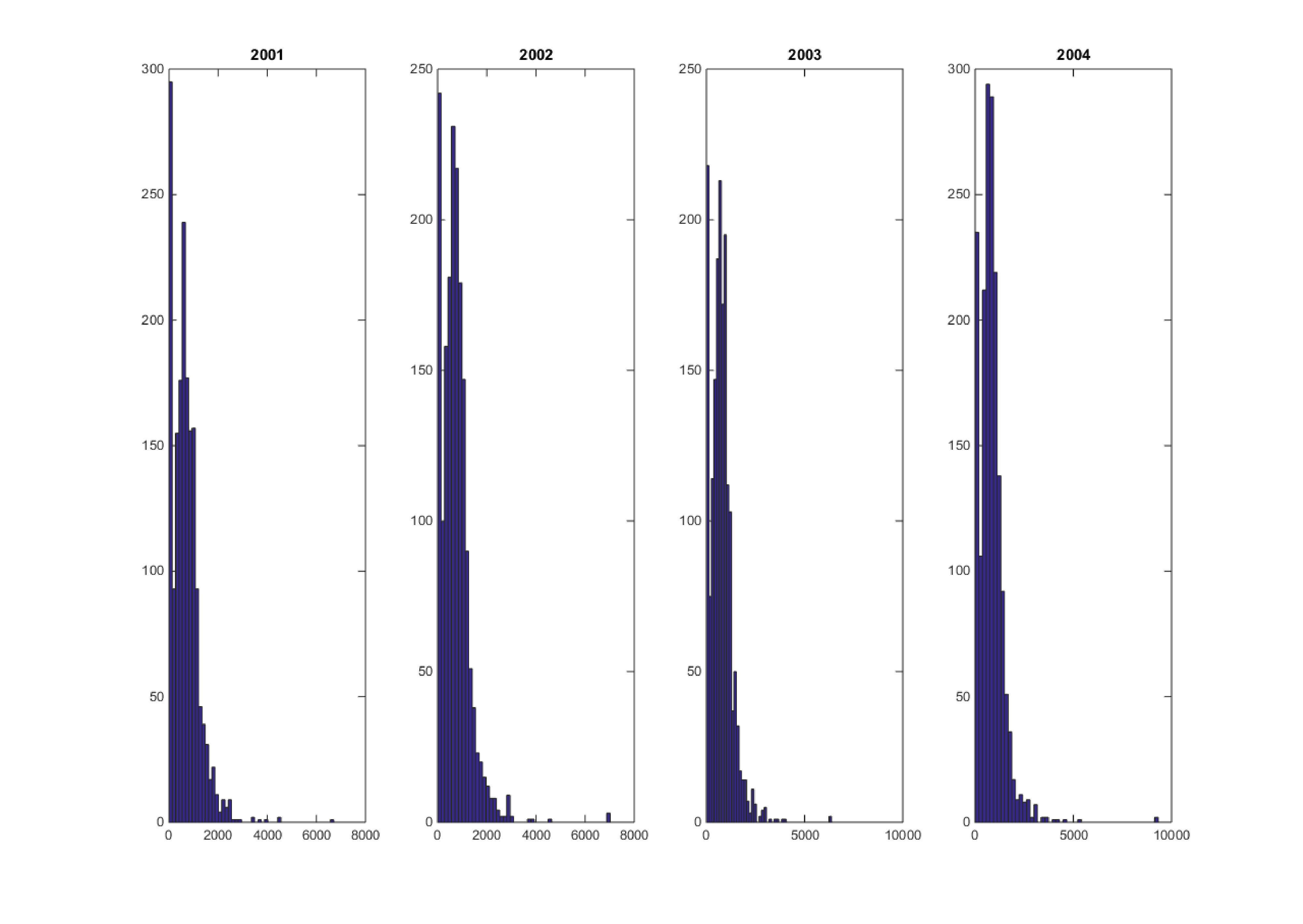
Figure S2: Histogram of real individual wages ($) for Australia in 2001, 2002, 2003, and 2004 respectively from left to right

Although a number of income related variables are available, we use the imputed income series _WSCEI in this example. This variable contains the average individual weekly wage and salary incomes from all paid employment over the period considered. It is reported before taxation and governmental transfers. The income data were also adjusted to account for the effects of inflation using the Consumer Price Index data obtained from the Australian Bureau of Statistics, which is based in 2010 dollars. From these data, a dependence sample was constructed by establishing whether a particular individual had recorded an income in all the years. Individuals who only recorded incomes in some of the years being considered were removed. In addition, we also focus our attention on individuals who are in the labor force (both employed and unemployed). We found that 1745 individuals recorded an income for all 13 years. Table 1 summarizes the distributions of real individual disposable income in Australia for the years 2001 - 2013 and shows that all income distributions exhibit positive skewness and fat long right tails typical of income distributions. If the ordering of the distributions is judged on the basis of the means or the medians, the population becomes better off as it moves from 2001 to 2013, except between the period 2006 and 2007. These effects are also confirmed by Figures S2 to S4 in appendix S4

Table 1: Descriptive statistics for real individual wages for Australia for the years 2001 - 2013

	2001	2002	2003	2004	2005	2006	2007	2008	2009	2010	2011	2012	2013
Mean	684	734	766	819	874	923	783	1067	1105	1128	1188	1215	1245
Median	616	673	712	753	803	852	702	969	1003	1048	1051	1101	1100
Std. dev.	551	591	568	645	674	668	694	788	825	869	990	916	950
skewness	2.1	3.0	2.1	3.7	2.9	1.5	2.0	2.0	1.8	2.0	3.7	1.9	1.5
kurtosis	15.7	26.6	16.0	40.2	27.1	8.7	11.1	12.7	11.7	15.7	37.5	13.0	7.4

4.1 Foster’s (2009) Chronic Poverty Measures

The measurement of chronic income poverty is important because it focuses on those whose lack of income stops them from obtaining the “minimum necessities of life” for much of their life course. Let $z\in\mathbb{R^{+}}$ be the poverty line. It is the level of income/wages which is just sufficient for someone to be able to afford the minimum necessities of life. For every $i=1,...,n$ and $t=1,...,T$, the row vector $\mathbf{y}_{i}=\left(y_{i1},...,y_{iT}\right)$ contains individual $i$’s incomes across time and the column vector $\mathbf{y}_{*t}=\left(y_{1t},...,y_{nt}\right)^{{}^{\prime}}$ contains the income distribution at period $t$.

The measurement of chronic poverty is split into two steps: an “identification” step and an aggregation step. The identification function $\rho\left(\mathbf{y}_{i};z\right)$ indicates that individual $i$ is in chronic poverty when $\rho\left(\mathbf{y}_{i};z\right)=1$, while $\rho\left(\mathbf{y}_{i};z\right)=0$ otherwise. Foster (2009) proposed an identification method that counts the number of periods of poverty experienced by a particular individual, $y_{it}\char 60\relax z$, and then expressed it as a fraction $d_{i}$ of the $T$ periods. The identification function $\rho_{\tau}\left(\mathbf{y}_{i};z\right)=1$ if $d_{i}\geq\tau$ and $\rho_{\tau}\left(\mathbf{y}_{i};z\right)=0$ if $d_{i}\char 60\relax\tau$.

The aggregation step combines the information on the chronically poor people to obtain an overall level of chronic poverty in a given society. We use the extension of univariate Foster, Greer and Thorbecke (FGT) poverty indices of Foster et al. (1984). These are given by

$$FGT^{\alpha}\left(z\right)=\frac{1}{n}\sum_{i=1}^{n}g_{i}^{\alpha}\ ,$$

where $g_{i}^{\alpha}=0$ if $y_{i}\char 62\relax z$ and $g_{i}^{\alpha}\left(z\right)=\left(\frac{z-y_{i}}{z}\right)^{\alpha}$ if $y_{i}\leq z$, and $\alpha$ measures inequality aversion. The FGT measure when $\alpha=0$ is called the headcount ratio, when $\alpha=1$ it is called the poverty gap index and when $\alpha=2$ it is called the poverty severity index. Foster (2009) proposed duration adjusted FGT poverty indices: duration adjusted headcount ratio and duration adjusted poverty gap. Following Foster (2009), we define the normalized gap matrix as $G^{\alpha}\left(z\right):=\left[g_{it}^{\alpha}\left(z\right)\right]$, where $g_{it}^{\alpha}\left(z\right)=0$ if $y_{it}\char 62\relax z$ and $g_{it}^{\alpha}\left(z\right)=\left(\frac{z-y_{it}}{z}\right)^{\alpha}$ if $y_{it}\leq z$. Then, identification is incorporated into the censored matrix $G^{\alpha}\left(z,\tau\right)=\left[g_{it}^{\alpha}\left(z,\tau\right)\right]$, where $g_{it}^{\alpha}\left(z,\tau\right)=g_{it}^{\alpha}\left(z\right)\rho_{\tau}\left(\mathbf{y}_{i};z\right)$. The entries for the non-chronically poor are censored to zero, while the entries for the chronically poor are left unchanged. When $\alpha=0$, the measure becomes the duration adjusted headcount ratio and is the mean of $G^{0}\left(z,\tau\right)$, and when $\alpha=1$, the measure becomes the duration adjusted poverty gap, and is given by the mean of $G^{1}\left(z,\tau\right)$.

4.2 Shorrocks (1978a) Income Mobility Measures

The measurement of income mobility focuses on how individuals’ income changes over time. Many mobility measures have been developed and applied to empirical data to describe income dynamics; see Shorrocks (1978b), Shorrocks (1978a), Formby et al. (2004), Dardanoni (1993), Fields and Ok (1996), Maasoumi and Zandvakili (1986), and references therein. However, statistical inference on income mobility has been largely neglected in the literature. Only recently, some researchers have developed statistical inference procedures for the measurement of income mobility (Biewen, 2002; Maasoumi and Trede, 2001; Formby et al., 2004). Here, we show that our approach can be used to obtain the posterior densities of mobility measures which can then be used for making inference on income mobility.

Shorrocks (1978b) proposed a measure of income mobility that is based on transition matrices. Following Formby et al. (2004), we consider the joint distribution of two income variables $y_{1}$ and $y_{2}$ with a continuous CDF $F\left(y_{1},y_{2}\right)$. This distribution function captures all the transitions between $y_{1}$ and $y_{2}$. In this application, we consider the mobility between two points in time. The movement between $y_{1}$ and $y_{2}$ is described by a transition matrix. To form the the transition matrix from $F\left(y_{1},y_{2}\right)$, we need to determine the number of, and boundaries between, income classes. Suppose there are $m$ classes in each of the income variables and the boundaries of these classes are $0\char 60\relax\tau_{1}^{y_{1}}\char 60\relax...\char 60\relax\tau_{m-1}^{y_{1}}\char 60\relax\infty$ and $0\char 60\relax\tau_{1}^{y_{2}}\char 60\relax...\char 60\relax\tau_{m-1}^{y_{2}}\char 60\relax\infty$. The resulting transition matrix is denoted $P=\left[p_{ij}\right]$. Each element $p_{ij}$ is a conditional probability that an individual moves to class $j$ of income $y_{2}$ given that they are initially in class $i$ with income $y_{1}$. It is defined as

$$p_{ij}:=\frac{\Pr\left(\tau_{i-1}^{y_{1}}\leq y_{1}\char 60\relax\tau_{i}^{y_{1}}\;and\;\tau_{j-1}^{y_{2}}\leq y_{2}\char 60\relax\tau_{j}^{y_{2}}\right)}{\Pr\left(\tau_{i-1}^{y_{1}}\leq y_{1}\char 60\relax\tau_{i}^{y_{1}}\right)}\ ,$$

where $\Pr\left(\tau_{i-1}^{y_{1}}\leq y_{1}\char 60\relax\tau_{i}^{y_{1}}\right)$ is the probability that an individual falls into income class $i$ of $y_{1}$.

A Mobility measure $M\left(P\right)$ can be defined as a function of the transition matrix $P$. We say that a society with transition matrix $P_{1}$ is more mobile than one with transition matrix $P_{2}$, according to mobility measure $M\left(P\right)$, if and only if $M\left(P_{1}\right)\char 62\relax M\left(P_{2}\right)$. We consider a mobility measure developed by Shorrocks (1978b) and defined as

$$M_{1}\left(P\right):=\frac{m-\sum_{i=1}^{m}p_{ii}}{m-1};$$

$M_{1}$ measures the average probability across all classes that an individual will leave his initial class in the next period.

4.3 Empirical Analysis

This section discusses the results from the analysis of the real individual wages data after estimating the proposed multivariate income distribution model using a Bayesian approach. The univariate income distribution is usually modeled using Dagum or Singh-Maddala distributions (Kleiber, 1996). In this example, the marginal income distribution is modeled using empirical distribution function, for simplicity. It is straightforward to extend the MCMC sampling scheme in Section 3 to estimate both marginal and joint parameters as in Pitt et al. (2006) and Smith and Khaled (2012).

First, we present the model selection results and the estimated parameters of the copula models. To select the best copula model, we use the $DIC_{3}$ criterion of Celeux et al. (2006) and the cross-validated log predictive score (LPDS) (Good, 1952; Geisser, 1980). The $DIC_{3}$ criterion is defined as

$$DIC_{3}:=-4{\mathbb{E}}_{\theta}\left(\log p\left(\bm{y}|\theta\right)|\bm{y}\right)+2\log\widehat{p}\left(\bm{y}\right),$$

where $\widehat{p}\left(\bm{y}\right)=\prod_{i=1}^{n}\widehat{p}\left(y_{i}\right)$. We next define the $B$-fold cross-validated LPDS. Suppose that the dataset ${\cal D}$ is split into roughly $B$ equal parts ${\cal D}_{1},...,{\cal D}_{B}$. Then, the $B-$fold cross validated LPDS is defined as

$$LPDS\left(\widehat{p}\right):=\sum_{j=1}^{B}\sum_{y_{j}\in{\cal D}_{j}}\log\widehat{p}\left(\mathbf{y}_{j}|{\cal D}\setminus{\cal D}_{j}\right)$$

In our work we take $B=5$. Table 2 shows that the best model, according to both criteria, is the mixture of Gaussian, Clayton, and Gumbel copulas. We estimate the best model with an initial burnin period of 10000 sweeps and a Monte Carlo sample of 10000 iterates. Next, we use the iterates from the best model to estimate transition probabilities from 0 to positive wages and from positive wages to zero, Spearman’s correlation coefficient, and the mobility and poverty measures, by averaging over the posterior distribution of the parameters.

Table 3 shows some of the estimated parameters and corresponding 95% credible intervals for the chosen copula mixture model. The parameters and their 95% credible intervals are quite tight, indicating that the parameters are well estimated. It is clear that there are significant differences in the estimated parameters by taking into account the point mass at zero wages compared to the parameters estimated by not taking into account this point mass. The estimated mixture weight parameters show that the Gaussian copula has the highest weight, followed by the Clayton and Gumbel copulas. As the weight of the Clayton copula is higher than of the Gumbel copula, it implies that there are more people with lower tail dependence than upper tail dependence. This may coincide with a relatively higher degree of income mobility amongst high income earners.

Table 2: Model Selection of the copula to model 13 years of income distribution with point mass at zero incomes

Model	$DIC_{3}$	LPDS-CV
Clayton	$-1.21\times 10^{4}$	$6.03\times 10^{3}$
Gumbel	$-1.75\times 10^{4}$	$4.95\times 10^{3}$
Gaussian	$-2.13\times 10^{4}$	$4.29\times 10^{4}$
Mixture (Gaussian, Clayton)	$-2.86\times 10^{4}$	$5.63\times 10^{4}$
Mixture (Gaussian, Gumbel)	$-2.83\times 10^{4}$	$5.54\times 10^{4}$
Mixture (Clayton, Gumbel)	$-1.68\times 10^{4}$	$3.31\times 10^{4}$
Mixture (Gaussian, Clayton, Gumbel)	$-2.89\times 10^{4\star}$	$5.68\times 10^{4\star}$

Table 3: Some of the estimated parameters of the mixture of the Gaussian, Gumbel and Clayton copulas to model 13 years of income distributions. The 95% credible intervals are in brackets

Parameters	Copula (Point Mass)	Copula (No Point Mass)
$\theta_{Cl}$	$\underset{\left(0.12,0.18\right)}{0.15}$	$\underset{\left(0.29,0.37\right)}{0.33}$
$\theta_{Gu}$	$\underset{\left(1.84,2.06\right)}{1.94}$	$\underset{\left(2.23,2.45\right)}{2.33}$
$w_{1}$	$\underset{\left(0.64,0.69\right)}{0.66}$	$\underset{\left(0.60,0.65\right)}{0.62}$
$w_{2}$	$\underset{\left(0.19,0.24\right)}{0.21}$	$\underset{\left(0.21,0.26\right)}{0.23}$

Tables S1 and S2 in Appendix S4 present the estimates of the transition probabilities from 0 to positive wages and from positive to 0 wages. The estimates of the transition probabilities seem to be close to their sample (non-parametric) counterparts. The estimates of transition probabilities from 0 to positive wages are similar (0.39-0.49) in the period from 2001-2006. Similarly, the estimates are similar in the period 2008-2013 (0.34-0.38). However, there are higher estimates for the period 2006-2007 and 2007-2008 (0.83 and 0.87, respectively). Similar results are observed for the transition probabilities from positive to zero wages. The estimates of the transition probabilities are roughly the same between the periods 2001-2006 and 2008-2013. There are higher estimates for the period 2006-2007 and 2007-2008. This phenomenon may indicate that there is very high income mobility between 2006-2007 and 2007-2008. Note that the model that does not take into account the point masses at zero cannot give us the estimate of transition probabilities.

Tables 4 and 5 show the estimate of Spearman’s rho dependence and Shorrocks (1978b) mobility measure. We can see from these two measures that there are very high values of the mobility measure and very low values of Spearman’s rho dependence measure between 2006-2007 and 2007-2008. This confirms our previous analysis that in the period 2006-2008 there is very high mobility between income earners. Table 6 shows the estimates of Foster’s chronic poverty measures: duration adjusted headcount ratio and duration adjusted poverty gap. The two measures indicate that the chronic poverty is significantly lower in the 2007-2013 period compared to the 2001-2006 period. The standard of living in Australia is higher in the period 2007-2013 compared to the period 2001-2006. Furthermore, we can see that the estimates of Spearman’s rho dependence, mobility, and chronic measures are different between the estimates that take into account the point masses and the estimates that do not take into account the point masses at zero wages. Figure 1 shows the posterior densities of duration adjusted headcount ratio for the years 2007-2013 for the two estimates. The figure shows that the posterior densities almost do not overlap, indicating that the two estimates are significantly different. Therefore, whenever the point masses are present, it is strongly recommended to incorporate them into the model to guard against biased estimates.

Table 4: Estimates of the Spearman rho dependence measure of the mixture of the Gaussian, Gumbel and Clayton copulas and 95% credible intervals (in brackets)

Period	Copula (Point Mass)	Copula (No Point Mass)
2001-2002	$\underset{\left(0.684,0.722\right)}{0.703}$	$\underset{\left(0.723,0.757\right)}{0.740}$
2002-2003	$\underset{\left(0.700,0.737\right)}{0.719}$	$\underset{\left(0.726,0.759\right)}{0.743}$
2003-2004	$\underset{\left(0.702,0.739\right)}{0.721}$	$\underset{\left(0.727,0.759\right)}{0.743}$
2004-2005	$\underset{\left(0.7040,0.741\right)}{0.723}$	$\underset{\left(0.730,0.763\right)}{0.747}$
2005-2006	$\underset{\left(0.708,0.745\right)}{0.727}$	$\underset{\left(0.733,0.766\right)}{0.750}$
2006-2007	$\underset{\left(-0.028,0.068\right)}{0.020}$	$\underset{\left(-0.020,0.086\right)}{0.030}$
2007-2008	$\underset{\left(-0.023,0.073\right)}{0.025}$	$\underset{\left(-0.013,0.093\right)}{0.037}$
2008-2009	$\underset{\left(0.706,0.744\right)}{0.725}$	$\underset{\left(0.733,0.766\right)}{0.7500}$
2009-2010	$\underset{\left(0.716,0.753\right)}{0.735}$	$\underset{\left(0.741,0.775\right)}{0.758}$
2010-2011	$\underset{\left(0.720,0.758\right)}{0.740}$	$\underset{\left(0.747,0.781\right)}{0.764}$
2011-2012	$\underset{\left(0.718,0.755\right)}{0.737}$	$\underset{\left(0.745,0.778\right)}{0.762}$
2012-2013	$\underset{\left(0.714,0.752\right)}{0.733}$	$\underset{\left(0.742,0.776\right)}{0.759}$

Table 5: Estimates of Shorrocks (1978a) Mobility Measure ($m=5$) of the mixture of the Gaussian, Gumbel and Clayton copulas

Period	Non-Parametric	Copula (Point Mass)	Copula (No Point Mass)
2001-2002	$\underset{\left(0.367,0.466\right)}{0.414}$	$\underset{\left(0.549,0.588\right)}{0.569}$	$\underset{\left(0.501,0.534\right)}{0.518}$
2002-2003	$\underset{\left(0.361,0.461\right)}{0.411}$	$\underset{\left(0.508,0.543\right)}{0.526}$	$\underset{\left(0.484,0.516\right)}{0.499}$
2003-2004	$\underset{\left(0.324,0.409\right)}{0.366}$	$\underset{\left(0.483,0.516\right)}{0.500}$	$\underset{\left(0.463,0.495\right)}{0.479}$
2004-2005	$\underset{\left(0.341,0.418\right)}{0.380}$	$\underset{\left(0.473,0.506\right)}{0.489}$	$\underset{\left(0.450,0.480\right)}{0.465}$
2005-2006	$\underset{\left(0.352,0.427\right)}{0.392}$	$\underset{\left(0.468,0.5000\right)}{0.484}$	$\underset{\left(0.444,0.475\right)}{0.459}$
2006-2007	$\underset{\left(0.974,1.019\right)}{0.996}$	$\underset{\left(0.957,0.980\right)}{0.969}$	$\underset{\left(0.878,0.938\right)}{0.918}$
2007-2008	$\underset{\left(0.959,1.015\right)}{0.987}$	$\underset{\left(0.921,0.945\right)}{0.933}$	$\underset{\left(0.843,0.906\right)}{0.885}$
2008-2009	$\underset{\left(0.384,0.441\right)}{0.411}$	$\underset{\left(0.493,0.526\right)}{0.510}$	$\underset{\left(0.465,0.495\right)}{0.480}$
2009-2010	$\underset{\left(0.350,0.409\right)}{0.380}$	$\underset{\left(0.482,0.516\right)}{0.500}$	$\underset{\left(0.449,0.481\right)}{0.465}$
2010-2011	$\underset{\left(0.351,0.411\right)}{0.381}$	$\underset{\left(0.463,0.500\right)}{0.481}$	$\underset{\left(0.424,0.456\right)}{0.440}$
2011-2012	$\underset{\left(0.353,0.405\right)}{0.380}$	$\underset{\left(0.475,0.510\right)}{0.492}$	$\underset{\left(0.437,0.469\right)}{0.453}$
2012-2013	$\underset{\left(0.339,0.395\right)}{0.365}$	$\underset{\left(0.499,0.536\right)}{0.517}$	$\underset{\left(0.458,0.493\right)}{0.475}$

Table 6: Estimates of Foster’s chronic poverty measure of the mixture of the Gaussian, Gumbel and Clayton copulas with 95% credible intervals (in brackets)

Measure	Period	Non-Parametric	Copula (Point Mass)	Copula (No Point Mass)
adj. headcount	2001-2006	$\underset{\left(0.193,0.229\right)}{0.211}$	$\underset{\left(0.187,0.197\right)}{0.192}$	$\underset{\left(0.197,0.205\right)}{0.201}$
adj. headcount	2007-2013	$\underset{\left(0.120,0.149\right)}{0.135}$	$\underset{\left(0.123,0.130\right)}{0.126}$	$\underset{\left(0.131,0.138\right)}{0.135}$
adj. poverty gap	2001-2006	$\underset{\left(0.123,0.150\right)}{0.137}$	$\underset{\left(0.130,0.137\right)}{0.134}$	$\underset{\left(0.137,0.144\right)}{0.141}$
adj. poverty gap	2007-2013	$\underset{\left(0.095,0.119\right)}{0.108}$	$\underset{\left(0.101,0.107\right)}{0.104}$	$\underset{\left(0.108,0.114\right)}{0.111}$

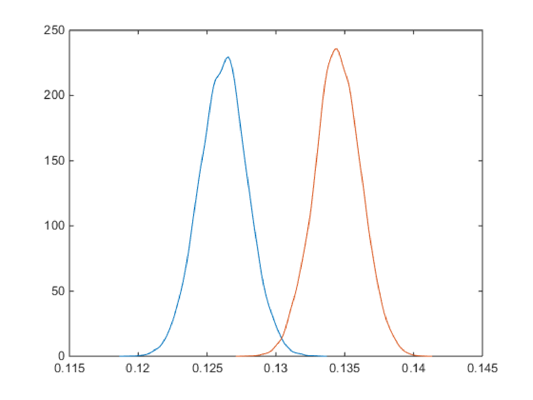
Figure 1: Estimated headcount posterior densities based on including (left density-blue line) and not including point masses (right density-orange line) at 0 (2007-2013)

5 Conclusion and discussion

The paper shows how to define and derive the density of the observations of a general copula model when some of the marginals are discrete, some are continuous and some of the marginals are a mixture of discrete and continuous components. This is done by carefully defining the likelihood as the density of the observations with respect to a mixed measure and allows us to define the likelihood for general copula models and hence carry out likelihood based inference. Our work extends in a very general way the current literature on likelihood based inference which focuses on copulas where each marginal is either discrete or continuous. The inference in the paper is Bayesian and we show how to construct an efficient MCMC scheme to estimate functionals of the posterior distribution. Although our discussion and examples focus on Gaussian and Archimedean copulas, our treatment is quite general and can be applied as long as it is possible to compute certain marginal and conditional copulas either in closed-form or numerically.

Our article can be extended in the following directions. First, using our definition of the likelihood also enables maximum likelihood type inference using, for example, simulated EM or simulated maximum likelihood. Second, copulas based on pair-copula constructions (e.g. Aas et al., 2009) or vine copulas (e.g. Bedford and Cooke, 2002) lend themselves well to our approach because the methods in this paper apply to arbitrary copulas with the only requirement that it is possible to write down several conditional marginal copulas and copula densities and being able to compute those either analytically or numerically. Third, by using pseudo marginal methods (e.g. Andrieu et al., 2010), our methodology can also be extended to the case where the case where the likelihood of the copula can only be estimated unbiasedly, rather than evaluated. We leave all such extensions to future work.

Our article illustrates the methodology and algorithms by applying them to estimate a multivariate income dynamics model. Examples of further possible applications arise from any setup where one or more of the following variables are present: wages (where there are points of probability mass at the minimum wage) individual sales figures, where there is a point of probability mass at 0 (many individuals deciding not to purchase) and a smooth distribution above that point (corresponding to a continuum of price figures). Another interesting potential application is to extend the general truncated/censored variable models in econometrics to a copula framework, e.g., for multivariate tobit and sample selection models.

Appendix A Difference operator notation

Since the difference operator notation can be easily confusing, it is useful to adopt the convention below. The notation has two components:

1. Whenever the $\bigtriangleup$ operators are applied to a function, an indexing is used to make the domain of the function clear.

2. A dot marks the position of the variables that are being differenced.

Here are some examples to illustrate the use of that notation.

• Consider a function $g(x)$ where $x$ is a scalar. Then $\bigtriangleup_{a}^{b}g_{x}(\cdot)$ defines

  $$\bigtriangleup_{a}^{b}g_{x}(\cdot):=g(b)-g(a)$$

• Consider a function $g(x,y)$ where both $x$ and $y$ are scalars. By $\bigtriangleup_{a}^{b}g_{x,y}(\cdot,z)$ we mean that the differencing is only applied to $x$ while the second argument is fixed at $y=z$, that is

  $$\bigtriangleup_{a}^{b}g_{x,y}(\cdot,z):=g(b,z)-g(a,z)$$

• Consider a function $g(\bm{x})$ where $\bm{x}$ is two-dimensional. By $\bigtriangleup_{\bm{a}}^{\bm{b}}g_{\bm{x}}(\cdot)$, we mean

  $$\bigtriangleup_{\bm{a}}^{\bm{b}}g_{\bm{x}}(\cdot) = \bigtriangleup_{a_{1}}^{b_{1}}\bigtriangleup_{a_{2}}^{b_{2}}g_{\bm{x}}(\cdot)$$

  $$= \bigtriangleup_{a_{1}}^{b_{1}}(g_{x_{1},x_{2}}(\cdot,b_{2})-g_{x_{1},x_{2}}(\cdot,a_{2}))$$

  $$= g(b_{1},b_{2})-g(b_{1},a_{2})-g(a_{1},b_{2})+g(a_{1},a_{2})$$

• Consider a function $g(\bm{x},\bm{y})$. If the differencing is applied to $\bm{y}$ and not $\bm{x}$, and if $\bm{y}$ is two-dimensional, then $\bigtriangleup_{\bm{a}}^{\bm{b}}g_{\bm{x},\bm{y}}(\bm{x},\cdot)$ means

  $$\bigtriangleup_{\bm{a}}^{\bm{b}}g_{\bm{x},\bm{y}}(\bm{x},\cdot) := \bigtriangleup_{a_{1}}^{b_{1}}\bigtriangleup_{a_{2}}^{b_{2}}g_{\bm{x},\bm{y}}(\bm{x},\cdot)$$

  $$= \bigtriangleup_{a_{1}}^{b_{1}}(g_{\bm{x},y_{1},y_{2}}(\bm{x},\cdot,b_{2})-g_{\bm{x},y_{1},y_{2}}(\bm{x},\cdot,b_{2}))$$

  $$= g(\bm{x},b_{1},b_{2})-g(\bm{x},a_{1},b_{2})-g(\bm{x},a_{2},b_{1})+g(\bm{x},a_{1},a_{2})$$

Appendix B Deriving the likelihood and the conditional density

This appendix deals with densities defined with respect to mixed measures. Such densities are formally defined by Radon-Nikodym derivatives. In particular, we obtain the joint density (1) of $\bm{X}$ and $\bm{U}$ and the corresponding mixed measure. We then show how to obtain the closed-form formulas for the densities (2) and (3), and their corresponding mixed measures, from the density (1).

We need the following three elementary lemmas to obtain the results. They are likely to be known in the literature, but we include their proofs for completeness.

Lemma 1.

Let $F(\bm{x},\bm{y})$ be the distribution function of an absolutely continuous random vector $(\bm{X}^{\prime},\bm{Y}^{\prime})^{\prime}$ where $\bm{x}\in\text{R}^{k}$ and $\bm{y}\in\text{R}^{p}$. Then,

$$\frac{\partial^{k}F(\bm{x},\bm{y})}{\partial x_{1}\cdots\partial x_{k}}=F(\bm{y}|\bm{x})f(\bm{x}),$$

where $F(\bm{y}|\bm{x})$ and $f(\bm{x})$ are respectively the distribution function of $\bm{Y}$ conditional on $\bm{X}=\bm{x}$ and the density of $\bm{X}$. Similarly, in an obvious notation,

$$\frac{\partial^{p}F(\bm{x},\bm{y})}{\partial y_{1}\cdots\partial y_{p}}=F(\bm{x}|\bm{y})f(\bm{y}).$$

Proof.

The identity comes from

$$\frac{\partial^{p}}{\partial y_{1}\cdots\partial y_{p}}F(\bm{y}|\bm{x})=f(\bm{y}|\bm{x})=\frac{f(\bm{y},\bm{x})}{f(\bm{x})}=\frac{\frac{\partial^{p+k}F(\bm{x},\bm{y})}{\partial y_{1}\cdots\partial y_{p}\partial x_{1}\cdots\partial x_{k}}}{f(\bm{x})}=\frac{\partial^{p}}{\partial y_{1}\cdots\partial y_{p}}\left(\frac{\frac{\partial^{k}F(\bm{x},\bm{y})}{\partial x_{1}\cdots\partial x_{k}}}{f(\bm{x})}\right).$$

∎

The next lemma is an immediate consequence of the previous lemma.

Lemma 2.

Let $f(\bm{x},\bm{y})$ be the density of an absolutely continuous random vector $(\bm{X}^{\prime},\bm{Y}^{\prime})^{\prime}$ where $\bm{x}\in\text{R}^{k}$ and $\bm{y}\in\text{R}^{p}$ then

$$\int_{a_{1}}^{b_{1}}\cdots\int_{a_{k}}^{b_{k}}f(\bm{x},\bm{y})\mathrm{d}x_{1}\ldots\mathrm{d}x_{k}=\bigtriangleup_{a_{1}}^{b_{1}}\cdots\bigtriangleup_{a_{k}}^{b_{k}}F_{\bm{Y}|\bm{X}}(\bm{y}|.)f_{\bm{X}}(.)$$

where $F(\bm{y}|\bm{x})$ and $f(\bm{x})$ are respectively the conditional distribution function of $\bm{Y}$ on $\bm{X}=\bm{x}$ and the density of $\bm{X}$.

Proof.

Write the density function

$$f(\bm{x},\bm{y}) = \frac{\partial^{p+k}F(\bm{x},\bm{y})}{\partial y_{1}\cdots\partial y_{p}\partial x_{1}\cdots\partial x_{k}}$$

$$= \frac{\partial^{k}}{\partial x_{1}\cdots\partial x_{k}}\left(\frac{\partial^{p}F(\bm{x},\bm{y})}{\partial y_{1}\cdots\partial y_{p}}\right)$$

$$= \frac{\partial^{k}}{\partial x_{1}\cdots\partial x_{k}}(F(\bm{x}|\bm{y})f(\bm{y}))$$

where the last line follows from the previous lemma. The desired result follows by an application of the fundamental theorem of calculus. ∎

Lemma 3.

Suppose that $U$ is uniformly distributed on $[0,1]$.

1. Suppose that $X$ is a univariate random variable with CDF $F(x)$ that has an inverse and a density $f(x)$. Then, ${\mathrm{d}}u\delta_{F^{-1}(u)}({\mathrm{d}}x)=\delta_{F(x)}({\mathrm{d}}u)f(x){\mathrm{d}}x$, where ${\mathrm{d}}u,{\mathrm{d}}x$ are Lebesgue measures.

2. Suppose that $X$ is a discrete univariate random variable with support on the discrete set $I=\{x\}$. Then, ${\mathrm{d}}u\delta_{\{F(x^{-})\leq u\char 60\relax F(x)\}}({\mathrm{d}}x)={\cal{I}}\{u:F(x^{-})\leq u\char 60\relax F(x)\}{\mathrm{d}}u\delta_{I}({\mathrm{d}}x)$

The proofs of parts (i) and (ii) are in Section S3.

Suppose that the indices ${\cal M}_{\cal C}$ correspond to the continuous random variables, the indices ${\cal M}_{\cal D}$ to the discrete random variables and the indices ${\cal M}_{\cal J}$ to a mixture of discrete and continuous random variables. We define the joint density of $\bm{X}$ and $\bm{U}$ as

$$f(\bm{x},\bm{u}) :=c(\bm{u})\prod_{j\in{\cal M}_{\cal C}}{\cal{I}}(u_{j}=F_{j}(x_{j}))\prod_{j\in{\cal M}_{\cal D}}{\cal{I}}(F_{j}(x_{j}^{-})\leq u_{j}\char 60\relax F_{j}(x_{j}))\times$$

$$\prod_{j\in{\cal M}_{\cal J}}\big{(}{\cal{I}}(u_{j}=F_{j}(x_{j}))+{\cal{I}}(F_{j}(x_{j}^{-})\leq u_{j}\char 60\relax F_{j}(x_{j}))\big{)}$$ (14)

with respect to the measure

$${\mathrm{d}}\bm{u}\prod_{j\in{\cal M}_{\cal C}}\delta_{F_{j}^{-1}(u_{j})}({\mathrm{d}}x_{j})\prod_{j\in{\cal M}_{\cal D}}\delta_{F_{j}(x_{j}^{-})\leq u_{j}\char 60\relax F_{j}(x_{j})}({\mathrm{d}}x_{j})\times$$

$$\prod_{j\in{\cal M}_{\cal J}}\big{(}{\cal I}(u_{j}=F_{j}(x_{j})){\mathrm{d}}x_{j}+{\cal{I}}(F_{j}(x_{j}^{-})\leq u_{j}\char 60\relax F_{j}(x_{j}))\delta_{F_{j}(x_{j}^{-})\leq u_{j}\char 60\relax F_{j}(x_{j})}({\mathrm{d}}x_{j})\big{)}$$ (15)

Lemma 4.

1. Equation (1) gives the joint density of $\bm{X}$ and $\bm{U}$ at a given value $\bm{X}=\bm{x}$ and $\bm{U}=\bm{u}$.

2. Equation (2) is the marginal density of $\bm{X}$ at $\bm{X}=\bm{x}$.

3. Equation (3) is the conditional density of $\bm{U}_{{\cal D}(\bm{x})}$ given $\bm{X}=\bm{x}$.

Proof.

Part (i) follows directly from (B) and (B). Part (ii) follows by integrating out $\bm{u}$ using Lemma 2. Part (iii) follows from Lemma  3. ∎

Supplement to ‘Mixed marginal Coupula Modeling’

S1 Density, Conditional Distribution Function, and MCMC Sampling Methods for the Gaussian, Gumbel, and Clayton Copulas

S1.1 Gaussian copula

The Gaussian copula distribution and density function are given by Song (2000) as $C\left(u_{1},u_{2},...,u_{m};\Gamma\right)=\Phi_{m}\left(y_{1}^{*},y_{2}^{*},...,y_{m}^{*};\Gamma\right)$ and

$$c\left(u_{1},u_{2},...,u_{m};\Gamma\right) =|\Gamma|^{-1/2}\exp\left\{-\frac{1}{2}\mathbf{y}^{*^{\prime}}\left(\Gamma^{-1}-I\right)\mathbf{y}^{*}\right\},$$ (S1)

where $\mathbf{y}^{*}=\left(y_{1}^{*},y_{2}^{*},...,y_{m}^{*}\right)^{{}^{\prime}}$ and $y_{j}^{*}=\Phi^{-1}\left(F_{j}\left(y_{j};\bm{\theta}_{j}\right)\right)$ is the transformed Gaussian copula data; $\Phi_{m}\left(\right)$ is the distribution function of the standard $m$- dimensional multivariate Gaussian distribution $N\left(\mathbf{0},\Gamma\right)$ and $\Gamma$ is a correlation matrix. The correlation matrix $\Gamma$ captures the dependence among random variables $\mathbf{y}^{*}=\left(y_{1}^{*},y_{2}^{*},...,y_{m}^{*}\right)^{{}^{\prime}}$. There are $m\left(m-1\right)/2$ unknown parameters in the correlation matrix $\Gamma$. We can generate a random sample from the Gaussian copula as follows,

• Generate $z_{1},...,z_{m}$ from $N\left(0,\Gamma\right)$

• Compute a vector $\mathbf{u}=\left(\Phi\left(z_{1}\right),...,\Phi\left(z_{m}\right)\right)^{{}^{\prime}}$

• Compute $\mathbf{x}=\left(F_{1}^{-1}\left(u_{1}\right),...,F_{T}^{-1}\left(u_{m}\right)\right)^{{}^{\prime}}$

S1.2 Clayton and Gumbel copulas

The material in this section is covered in more detail in Hofert et al. (2012) and Cherubini et al. (2004). We consider a strict generator function

$$\psi\left(u\right):\left[0,1\right]\rightarrow\left[0,\infty\right]$$

which is continuous and strictly decreasing, with $\psi^{-1}$ completely monotonic on $\left[0,\infty\right]$. Then, the class of Archimedean copulas consists of copulas of the form (Cherubini et al., 2004)

$$C\left(\mathbf{u}\right)=C\left(u_{1},...,u_{m}\right)=\psi^{-1}\left(\psi\left(u_{1}\right)+...+\psi\left(u_{m}\right)\right).$$

A function $\psi$ on $\left[0,\infty\right]$ is the Laplace transform of a CDF $F$ if and only if $\psi$ is a completely monotonic and $\psi\left(0\right)=1$ and $\psi\left(\infty\right)=0$. Applying Bayesian methodology requires an efficient strategy to evaluate the density or the log-density of the parametric Archimedean copula family to be estimated. Although the density of an Archimedean copula has an explicit form in theory, it is often difficult to compute since computing the required derivatives is known to be extremely challenging, especially in high dimensional applications. Hofert et al. (2012) gives explicit formulae for the generator derivatives of the Archimedean family in any dimension. They also give an explicit formula for the density of some well-known Archimedean copulas, such as Ali-Mikhail-Haq, Clayton, Frank, Gumbel, and Joe copulas.

The generator for the Clayton copula is $\psi\left(u\right)=u^{-\theta}-1$ with $\psi^{-1}\left(t\right)=\left(1+t\right)^{-\frac{1}{\theta}}$. The CDF of the Clayton $m$-copula is

$$C\left(\mathbf{u}\right)=\left[\sum_{i=1}^{m}u_{i}^{-\theta}-m+1\right]^{-\frac{1}{\theta}},\theta\char 62\relax 0.$$

The dependence parameter $\theta$ is defined on the interval $\left(0,\infty\right)$. The Clayton copula favors data which exhibits strong lower tail dependence and weak upper tail dependence and thus is an appropriate choice of model if the data exhibits strong correlation at lower values and weak correlation at higher values. The density of the Clayton $m$-copula is

$$c\left(\mathbf{u}\right)=\prod_{k=0}^{m-1}\left(\theta k+1\right)\left(\prod_{j=1}^{m}u_{j}\right)^{-\left(1+\theta\right)}\left(\sum_{i=1}^{m}u_{i}^{-\theta}-m+1\right)^{-\left(m+\frac{1}{\theta}\right)}.$$

The generator of the Gumbel copula is $\psi\left(u\right)=\left(-\log\left(u\right)\right)^{\theta}$ with $\psi^{-1}\left(t\right)=\exp\left(-t^{\frac{1}{\theta}}\right)$. The Gumbel $m$-copula CDF is

$$C\left(\mathbf{u}\right)=\exp\left\{-\left[\sum_{i=1}^{m}\left(-\log\left(u_{i}\right)\right)^{\theta}\right]^{\frac{1}{\theta}}\right\}.$$

The dependence parameter $\theta$ is defined on the $\left[1,\infty\right)$ interval, where a value 1 represents the independence case. The Gumbel copula is an appropriate choice of model if the data exhibit weak correlation at lower values and strong correlation at the higher values. The density of the Gumbel $m$-copula is

$$c\left(\mathbf{u}\right)=\theta^{m}\exp\left\{-\left[\sum_{i=1}^{m}(-\log(u_{i}))^{\theta}\right]^{\frac{1}{\theta}}\right\}\times \frac{\prod_{j=1}^{m}(-\log u_{j})^{\theta-1}}{\left(\sum_{j=1}^{m}(-\log(u_{j}))^{\theta}\right)^{m}\prod_{j=1}^{m}u_{j}}$$

$$\times P_{d,\theta}^{G}\left(\left[\sum_{j=1}^{m}(-\log(u_{j}))^{\theta}\right]^{\frac{1}{\theta}}\right)$$

where,

$$P_{m,\theta}^{G}\left(x\right)=\sum_{k=1}^{m}a_{mk}^{G}\left(\theta\right)x^{k},$$

and

$$a_{mk}^{G}\left(\theta\right)=\frac{m!}{k!}\sum_{j=1}^{k}\left(\begin{array}[]{c}k\\ j\end{array}\right)\left(\begin{array}[]{c}j/\theta\\ m\end{array}\right)\left(-1\right)^{m-j}.$$

Marshall and Olkin (1988) proposed the following algorithm for sampling a $m$-dimensional exchangeable Archimedean copula with generator $\psi$.

• Sample $V\sim F=LS^{-1}\left(\psi^{-1}\right)$, where $LS^{-1}$ denotes the inverse Laplace-Stieljes transform of $\psi^{-1}$.

  • For the Clayton copula, $F=\varGamma\left(1/\theta,1\right)$, where $\varGamma\left(c,d\right)$ denotes the Gamma distribution with shape parameter $c\in\left(0,\infty\right)$, scale parameter $d\in\left(0,\infty\right)$

  • For the Gumbel copula, $F={\rm Stable}\left(1/\theta,1,\left(\cos\left(\frac{\pi}{2\theta}\right)\right)^{\theta},1;1\right)$,
    where $\rm{Stable}\left(\alpha_{st},\beta_{st},\gamma_{st},\delta_{st};1\right)$ denotes the Stable distribution with exponent $\alpha_{st}\in\left(0,2\right]$, skewness parameter $\beta_{st}\in\left[-1,1\right]$, scale parameter $\gamma_{st}\in\left[0,\infty\right)$, and location parameter $\delta_{st}\in\mathbb{R}$ (Nolan, 2007).

• Sample iid $X_{j}\sim U\left[0,1\right]$ for $j=1,...,m$

• Set $U_{j}=\psi\left(\frac{-\log\left(X_{j}\right)}{V}\right)$, for $t=1,...,T$

S1.3 Conditional posterior of the Gaussian Copula Parameters

At each iteration of the MCMC sampling scheme, the correlation matrix $\Gamma$ of the Gaussian copula is generated conditional on the transformed Gaussian copula variables $\mathbf{y}^{*}=\left\{y_{ij}^{*};i=1,...,n;\;j=1,...,m\right\}$. Danaher and Smith (2011) proposed the following representation of $\Gamma$,

$$\Gamma:={\rm diag}\left(\Sigma\right)^{-1/2}\;\Sigma\;\rm{diag}\left(\Sigma\right)^{-1/2},$$

where $\Sigma$ is a non-unique positive definite matrix and ${\rm diag}(\Sigma)$ is a diagonal matrix comprising the leading diagonal of $\Sigma$. The matrix $\Sigma$ is further decomposed into $\Sigma=R^{{}^{\prime}}R$, with $R$ an upper triangular Cholesky factor. If we set the leading diagonal of $R$ to ones, this leaves $m\left(m-1\right)/2$ unknown elements of $R$, matching the number of unknown elements of $\Gamma$, thus identifying the representation. The upper triangular elements of $R$ are unconstrained. The transformation described above ensures that the correlation matrix $\Gamma$ remains a positive definite matrix, regardless of the values of $R$.

The following steps generate each element of $R$:

1. Generate the $r_{j^{*}j}$ element of the matrix $R$ using a random-walk Metropolis step for $j^{*}=1,...,m$ and $j=2,...,m$ with $j^{*}\char 60\relax j$.

2. Compute $\Sigma=R^{{}^{\prime}}R$

3. Compute the correlation matrix $\Gamma={\rm diag}\left(\Sigma\right)^{-1/2}\Sigma{\rm diag}\left(\Sigma\right)^{-1/2}$

To explain step 1 in more detail, the conditional posterior $r_{j^{*}j}|\left\{R\setminus r_{j^{*}j}\right\},\mathrm{\mathbf{y}}^{*},\mathbf{y}$ is given by

$$p\left(r_{j^{*}j}|\left\{R\setminus r_{j^{*}j}\right\},\mathrm{\mathbf{y}}^{*},\mathbf{y}\right) \propto p\left(\mathrm{\mathbf{y}}|\mathbf{y}^{*}\right)p\left(\mathbf{y}^{*}|R\right)p\left(r_{j^{*}j}\right)$$

$$\propto \prod_{i=1}^{n}|\Gamma|^{-\frac{n}{2}}\exp\left\{-\frac{1}{2}\mathbf{y}_{i}^{*^{\prime}}\left(\Gamma^{-1}-I\right)\mathbf{y}_{i}^{*}\right\}p\left(r_{j^{*}j}\right),$$

with $p\left(r_{j^{*}j}\right)\propto 1$ for all elements of $R$. Here, $\left\{A\setminus B\right\}$ means $A$ with the parameters $B$ omitted. First, we generate a new proposal value, $r_{j^{*}j}^{*}$, from a candidate density $N\left(r_{j^{*}j},\sigma\right)$, where $r_{j^{*}j}$ is the previous iterate value and $\sigma$ is the pre-specified standard deviation of a normal distribution specified to obtain a reasonable acceptance rate of 0.3-0.4. The new value $r_{j^{*}j}^{*}$ is accepted with probability

$$\alpha=\min\left\{1,\frac{p\left(r_{j^{*}j}^{*}|\left\{R\setminus r_{j^{*}j}\right\},\mathrm{\mathbf{y}}^{*},\mathbf{y}\right)}{p\left(r_{j^{*}j}|\left\{R\setminus r_{j^{*}j}\right\},\mathrm{\mathbf{y}}^{*},\mathbf{y}\right)}\right\}.$$

We draw a random variable $u$ from $U\left(0,1\right)$; if $u\char 60\relax\alpha$, then the new value of $r_{j^{*}j}$ is accepted, otherwise the old value of $r_{j^{*}j}$ is retained. This algorithm is used to generate all of the upper triangular elements of $R$, one at a time.

S1.4 Generation of the latent variables

The following algorithm can be used to generate the latent variables one margin at a time.

• In the income application, the point mass occurs at zero wages.

• For $j=1,...,m$

  • for $i=1,...,n$

    • if $y_{ij}=0$

    • Compute $A_{ij}=C_{j|\left\{1,...,m\right\}\setminus ja}\left(b_{i,j}|\left\{u_{i1},...,u_{ij}\right\}\setminus u_{ij},\phi\right)$, then generate $w_{ij}\sim Uniform\left(0,A_{ij}\right)$

    • Compute $u_{ij}=C_{j|\left\{1,...,m\right\}\setminus j}^{-1}\left(w_{ij}|\left\{u_{i1},...,u_{im}\right\}\setminus u_{ij},\phi\right)$

S2 A trivariate example

This appendix uses a three dimensional example to illustrate the methods as some of the more complicated aspects of the methods may not be apparent in the two dimensional Example 1 discussed in Section 2. For brevity, the derivation is less detailed than that for Example 1.

Let $X_{1}$ have a distribution that is a mixture of two points of probability mass at zero and one and a normal distribution, that is let $X_{1}$ has the distribution function

$$F_{1}(x_{1})=(1-\pi_{1}-\pi_{2})\Phi(x_{1})+\pi_{1}\mathcal{I}(x_{1}\geqslant 0)+\pi_{2}\mathcal{I}(x_{1}\geqslant 1),$$

where $\Phi$ is the distribution function of a standard normal random variable. Let $X_{2}$ be a standard normal with a point of probability mass at $0$ and with distribution function

$$F_{2}(x_{2})=(1-\pi)\Phi(x)+\pi\mathcal{I}(x_{2}\geqslant 0).$$

Finally, let $X_{3}$ be a binary random variable.

This results in the following

$$\mathcal{C}(x_{1},x_{2},x_{3})=\left\{\begin{array}[]{lll}\{1,2\}&\mathrm{if}&x_{1}\not\in\{0,1\}\quad\mathrm{and}\quad x_{2}\not\in\{0\}\\ \{1\}&&x_{1}\not\in\{0,1\}\quad\mathrm{and}\quad x_{2}\in\{0\}\\ \{2\}&&x_{1}\in\{0,1\}\quad\mathrm{and}\quad x_{2}\not\in\{0\}\\ \varnothing&&x_{1}\in\{0,1\}\quad\mathrm{and}\quad x_{2}\in\{0\}\end{array}\right.$$

and $\mathcal{D}(x_{1},x_{2},x_{3})=\{1,2,3\}\backslash\mathcal{C}(x_{1},x_{2},x_{3})$. Notice that $\{3\}\subset\mathcal{D}(x_{1},x_{2},x_{3})$ always holds in this example.

The marginal density of $\mathbf{X}$ (Eq. 2 in the paper) is

1. Case 1: $\mathcal{C}(x_{1},x_{2},x_{3})=\{1,2\}$.

   $$f(\mathbf{x}) = c_{\{1,2\}}(\mathbf{b}_{\{1,2\}})f_{1}(x_{1})f_{2}(x_{2})\bigtriangleup_{a_{3}}^{b_{3}}C_{3|1,2}(\cdot|\mathbf{b}_{\{1,2\}})$$

   $$= c_{\{1,2\}}(\mathbf{b}_{\{1,2\}})f_{1}(x_{1})f_{2}(x_{2})(C_{3|1,2}(b_{3}|\mathbf{b}_{\{1,2\}})-C_{3|1,2}(a_{3}|\mathbf{b}_{\{1,2\}}))$$

2. Case 2: $\mathcal{C}(x_{1},x_{2},x_{3})=\{1\}$

   $$f(\mathbf{x}) = c_{1}(b_{1})f_{1}(x_{1})\bigtriangleup^{\mathbf{b}_{\{2,3\}}}_{\mathbf{a}_{\{2,3\}}}C_{2,3|1}(\cdot|b_{1})$$

   $$= f_{1}(x_{1})\times$$

   $$[C_{2,3|1}(b_{2},b_{3}|b_{1})-C_{2,3|1}(b_{2},a_{3}|b_{1})-C_{2,3|1}(a_{2},b_{3}|b_{1})+C_{2,3|1}(a_{2},a_{3}|b_{1})]$$

   where the second line follows from $c_{1}(b_{1})=1$ (as all one-dimensional marginals are uniform).

3. Case 3: $\mathcal{C}(x_{1},x_{2},x_{3})=\{2\}$

   $$f(\mathbf{x}) = c_{2}(b_{2})f_{2}(x_{2})\bigtriangleup^{\mathbf{b}_{\{1,3\}}}_{\mathbf{a}_{\{1,3\}}}C_{1,3|2}(\cdot|b_{2})$$

   $$= f_{2}(x_{2})\times$$

   $$[C_{1,3|2}(b_{1},b_{3}|b_{2})-C_{1,3|2}(b_{1},a_{3}|b_{2})-C_{1,3|2}(a_{1},b_{3}|b_{2})+C_{1,3|2}(a_{1},a_{3}|b_{2})]$$

4. Case 4: $\mathcal{C}(x_{1},x_{2},x_{3})=\varnothing$.

   $$f(\mathbf{x}) =C(b_{1},b_{2},b_{3})-C(a_{1},b_{2},b_{3})-C(b_{1},a_{2},b_{3})-C(b_{1},b_{2},a_{3})$$

   $$+C(a_{1},a_{2},b_{3})+C(a_{1},b_{2},a_{3})+C(b_{1},a_{2},a_{3})-C(a_{1},a_{2},a_{3})$$

In all the above, $b_{j}=F_{j}(x_{j})$ and $a_{j}=F_{j}(x_{j}^{-})$.

S3 Proof of Lemma 3

Proof.

• Suppose that $X$ is a univariate absolutely continuous random variable. Then the cumulative distribution function of $X$ is a strictly increasing $F$ and $U=F(X)$ will be uniformly distributed on the unit interval. The measure induced by $(X,U)$ is denoted by $\delta_{F(x)}(\mathrm{d}u)f(x)\mathrm{d}x$

  Let $h(x,u)$ be an integrable function of $x$ and $u$. Then, it is straightforward to check that

  $$\int\int h(x,u)f(x)\delta_{F(x)}(\mathrm{d}u)\mathrm{d}x =\int h(x,F(x))\mathrm{d}x=\int\int h(x,u)\mathrm{d}u\delta_{F^{-1}(u)}(\mathrm{d}x)$$

• The proof follows from the basic properties of a double integral because we can swap the order of integration. More formally, the proof follows from Theorem 3.1 (4) p.111 of Shorack (2000).

∎

S4 Some extra empirical results

This appendix includes additional plots for the analysis of the income dynamics data.

Table S1: Estimates of transition probabilities estimates of the mixture of the Gaussian, Gumbel and Clayton copulas taking into account the point masses at zero incomes and 95% credible intervals (in brackets)

Transition	0 to Positive Wages		Positive to 0 Wages
	Non-Parametric	Copula	Non-Parametric	Copula
2001-2002	$\underset{\left(0.388,0.531\right)}{0.465}$	$\underset{\left(0.477,0.507\right)}{0.492}$	$\underset{\left(0.031,0.050\right)}{0.040}$	$\underset{\left(0.042,0.046\right)}{0.044}$
2002-2003	$\underset{\left(0.290,0.434\right)}{0.361}$	$\underset{\left(0.391,0.423\right)}{0.407}$	$\underset{\left(0.035,0.055\right)}{0.045}$	$\underset{\left(0.048,0.052\right)}{0.050}$
2003-2004	$\underset{\left(0.234,0.379\right)}{0.313}$	$\underset{\left(0.383,0.414\right)}{0.398}$	$\underset{\left(0.032,0.053\right)}{0.043}$	$\underset{\left(0.051,0.054\right)}{0.053}$
2004-2005	$\underset{\left(0.245,0.391\right)}{0.316}$	$\underset{\left(0.389,0.419\right)}{0.404}$	$\underset{\left(0.031,0.049\right)}{0.041}$	$\underset{\left(0.049,0.053\right)}{0.051}$
2005-2006	$\underset{\left(0.216,0.341\right)}{0.280}$	$\underset{\left(0.372,0.402\right)}{0.387}$	$\underset{\left(0.030,0.051\right)}{0.040}$	$\underset{\left(0.052,0.055\right)}{0.053}$
2006-2007	$\underset{\left(0.842,0.930\right)}{0.886}$	$\underset{\left(0.811,0.845\right)}{0.828}$	$\underset{\left(0.130,0.163\right)}{0.148}$	$\underset{\left(0.138,0.142\right)}{0.140}$
2007-2008	$\underset{\left(0.866,0.936\right)}{0.900}$	$\underset{\left(0.854,0.880\right)}{0.868}$	$\underset{\left(0.094,0.126\right)}{0.111}$	$\underset{\left(0.103,0.107\right)}{0.106}$
2008-2009	$\underset{\left(0.220,0.346\right)}{0.283}$	$\underset{\left(0.340,0.372\right)}{0.356}$	$\underset{\left(0.043,0.065\right)}{0.054}$	$\underset{\left(0.061,0.065\right)}{0.063}$
2009-2010	$\underset{\left(0.210,0.322\right)}{0.267}$	$\underset{\left(0.329,0.360\right)}{0.344}$	$\underset{\left(0.040,0.062\right)}{0.051}$	$\underset{\left(0.060,0.065\right)}{0.062}$
2010-2011	$\underset{\left(0.262,0.380\right)}{0.321}$	$\underset{\left(0.361,0.390\right)}{0.375}$	$\underset{\left(0.032,0.053\right)}{0.043}$	$\underset{\left(0.050,0.054\right)}{0.052}$
2011-2012	$\underset{\left(0.230,0.356\right)}{0.294}$	$\underset{\left(0.367,0.3967\right)}{0.381}$	$\underset{\left(0.028,0.048\right)}{0.038}$	$\underset{\left(0.049,0.054\right)}{0.051}$
2012-2013	$\underset{\left(0.187,0.307\right)}{0.247}$	$\underset{\left(0.338,0.370\right)}{0.354}$	$\underset{\left(0.034,0.055\right)}{0.045}$	$\underset{\left(0.058,0.063\right)}{0.061}$

Table S2: Estimates of transition probabilities estimates of the mixture of the Gaussian, Gumbel and Clayton copulas taking into account the point masses at zero incomes and 95% credible intervals (in brackets)

Transition	Stay at 0		Stay at positive wages
	Non-Parametric	Copula	Non-Parametric	Copula
2001-2002	$\underset{\left(0.469,0.612\right)}{0.535}$	$\underset{\left(0.493,0.523\right)}{0.508}$	$\underset{\left(0.950,0.970\right)}{0.960}$	$\underset{\left(0.955,0.958\right)}{0.956}$
2002-2003	$\underset{\left(0.566,0.710\right)}{0.639}$	$\underset{\left(0.577,0.608\right)}{0.593}$	$\underset{\left(0.945,0.965\right)}{0.955}$	$\underset{\left(0.948,0.952\right)}{0.950}$
2003-2004	$\underset{\left(0.623,0.766\right)}{0.687}$	$\underset{\left(0.587,0.617\right)}{0.602}$	$\underset{\left(0.948,0.968\right)}{0.957}$	$\underset{\left(0.946,0.949\right)}{0.948}$
2004-2005	$\underset{\left(0.610,0.755\right)}{0.684}$	$\underset{\left(0.581,0.612\right)}{0.597}$	$\underset{\left(0.951,0.970\right)}{0.960}$	$\underset{\left(0.947,0.951\right)}{0.949}$
2005-2006	$\underset{\left(0.659,0.784\right)}{0.720}$	$\underset{\left(0.598,0.628\right)}{0.613}$	$\underset{\left(0.950,0.970\right)}{0.960}$	$\underset{\left(0.945,0.949\right)}{0.947}$
2006-2007	$\underset{\left(0.070,0.158\right)}{0.114}$	$\underset{\left(0.155,0.189\right)}{0.172}$	$\underset{\left(0.837,0.871\right)}{0.852}$	$\underset{\left(0.857,0.862\right)}{0.860}$
2007-2008	$\underset{\left(0.064,0.134\right)}{0.010}$	$\underset{\left(0.120,0.146\right)}{0.133}$	$\underset{\left(0.874,0.906\right)}{0.889}$	$\underset{\left(0.892,0.897\right)}{0.894}$
2008-2009	$\underset{\left(0.654,0.780\right)}{0.717}$	$\underset{\left(0.628,0.660\right)}{0.644}$	$\underset{\left(0.935,0.957\right)}{0.946}$	$\underset{\left(0.935,0.939\right)}{0.937}$
2009-2010	$\underset{\left(0.678,0.791\right)}{0.733}$	$\underset{\left(0.640,0.671\right)}{0.656}$	$\underset{\left(0.938,0.960\right)}{0.949}$	$\underset{\left(0.935,0.940\right)}{0.938}$
2010-2011	$\underset{\left(0.620,0.738\right)}{0.679}$	$\underset{\left(0.610,0.639\right)}{0.625}$	$\underset{\left(0.947,0.968\right)}{0.957}$	$\underset{\left(0.946,0.950\right)}{0.948}$
2011-2012	$\underset{\left(0.644,0.770\right)}{0.706}$	$\underset{\left(0.604,0.633\right)}{0.619}$	$\underset{\left(0.952,0.972\right)}{0.962}$	$\underset{\left(0.946,0.951\right)}{0.949}$
2012-2013	$\underset{\left(0.693,0.813\right)}{0.753}$	$\underset{\left(0.631,0.662\right)}{0.646}$	$\underset{\left(0.945,0.966\right)}{0.955}$	$\underset{\left(0.937,0.942\right)}{0.939}$

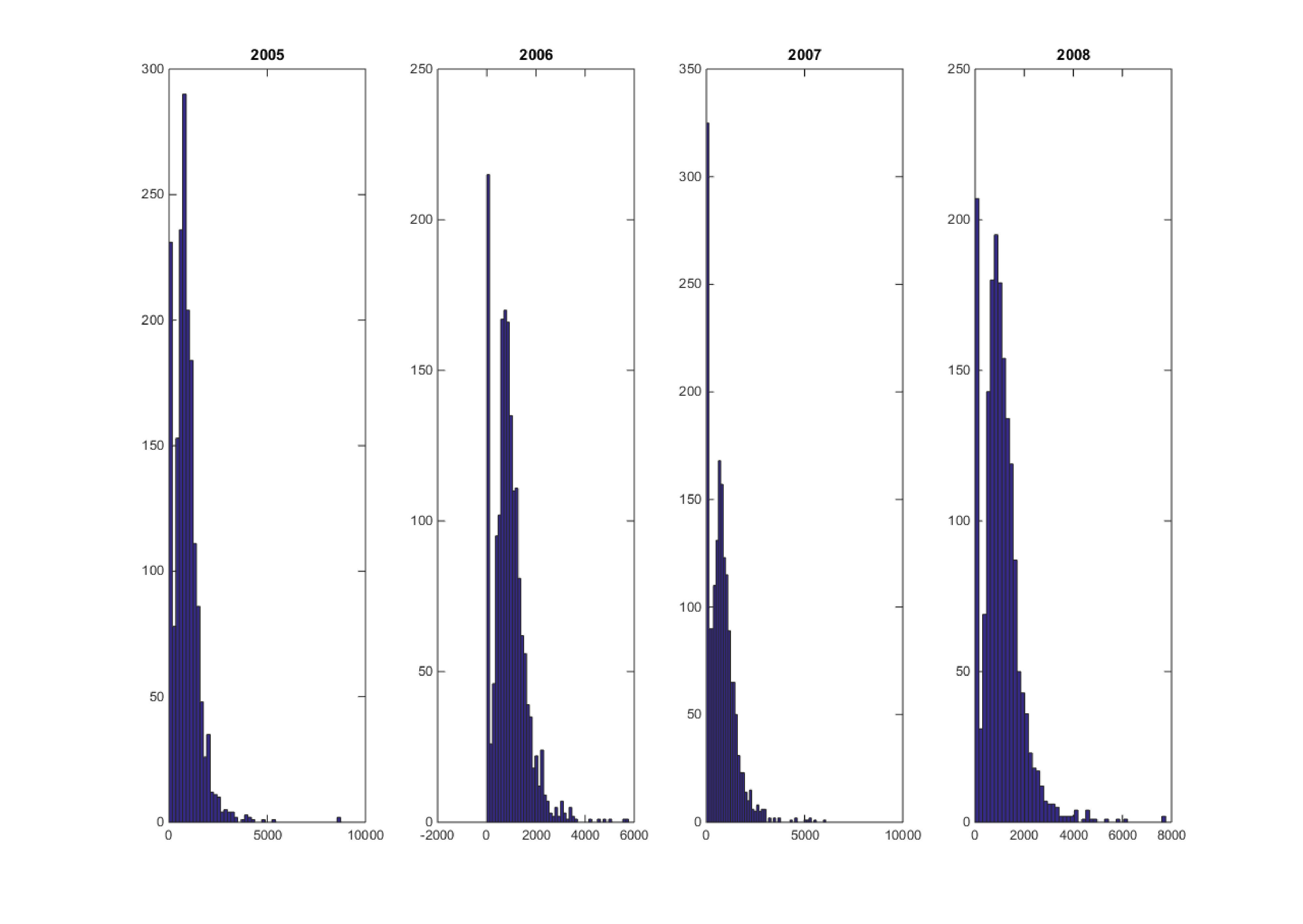
Figure S3: Histogram of real individual wages ($) for Australia in 2005, 2006, 2007, and 2008 respectively from left to right

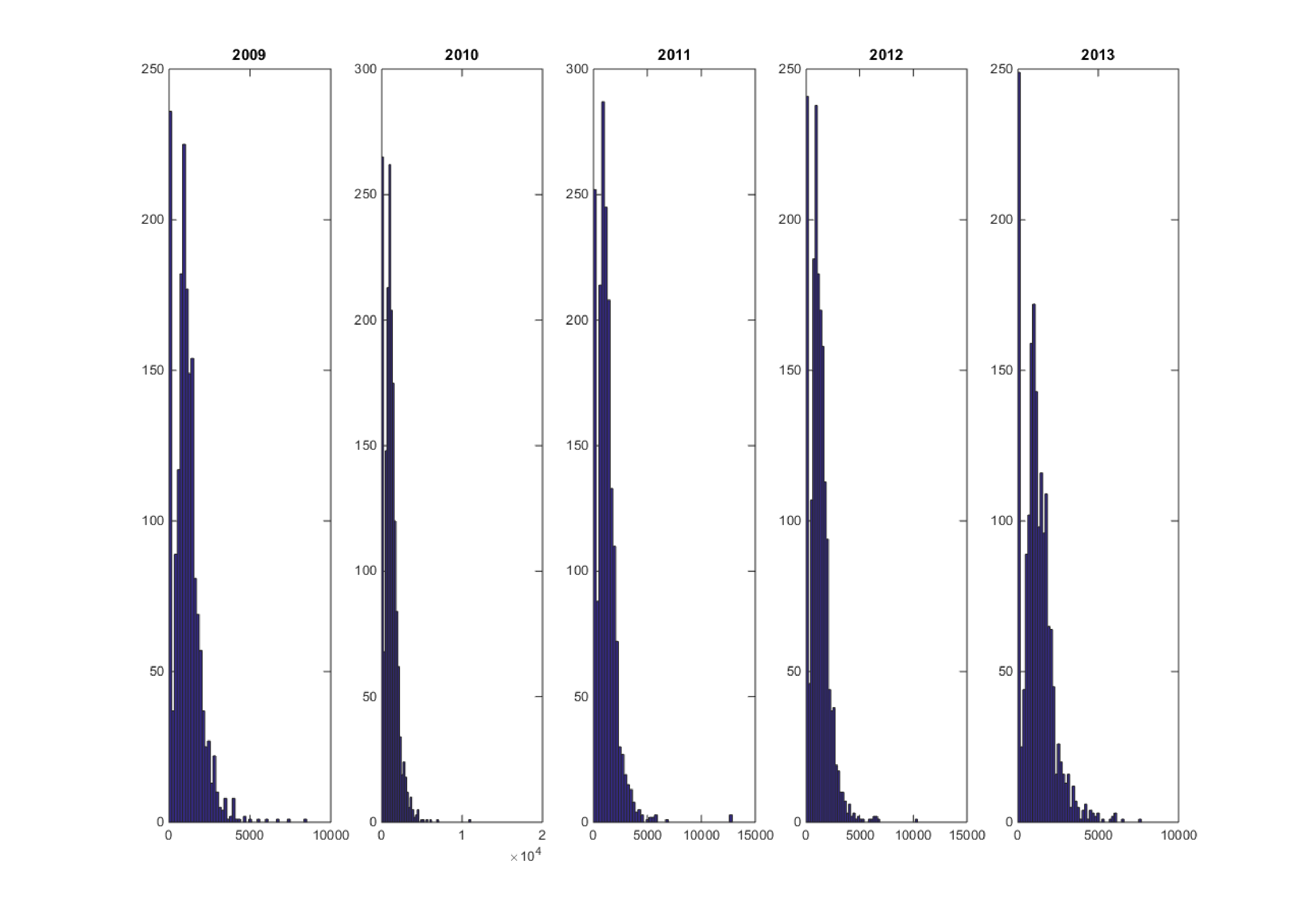
Figure S4: Histogram of real individual disposable wages ($) for Australia in 2009, 2010, 2011, 2012, and 2013 respectively from left to right

References

• Aas et al. (2009) Aas, K., Czado, C., Frigessi, A., and Bakken, H. (2009), “Pair-copula constructions of multiple dependence,” Insurance: Mathematics and economics, 44, 182–198.
• Andrieu et al. (2010) Andrieu, C., Doucet, A., and Holenstein, R. (2010), “Particle Markov chain Monte Carlo methods,” Journal of the Royal Statistical Society, Series B, 72, 1–33.
• Bedford and Cooke (2002) Bedford, T. and Cooke, R. M. (2002), “Vines: A new graphical model for dependent random variables,” Annals of Statistics, 1031–1068.
• Biewen (2002) Biewen, M. (2002), “Bootstrap Inference for Inequality, Mobility, and Poverty Measurement,” Journal of Econometrics, 108, 317–342.
• Bonhomme and Robin (2009) Bonhomme, S. and Robin, J.-M. (2009), “Assessing the equalizing force of mobility using short panels: France, 1990–2000,” The Review of Economic Studies, 76, 63–92.
• Brechmann et al. (2014) Brechmann, E., Czado, C., and Paterlini, S. (2014), “Flexible dependence modeling of operational risk losses and its impact on total capital requirements,” Journal of Banking & Finance, 40, 271–285.
• Celeux et al. (2006) Celeux, G., Forbes, F., Robert, C. P., and Titterington, D. M. (2006), “Deviance Information Criteria for Missing Data Models,” Bayesian Analysis, 1, 651–674.
• Cherubini et al. (2004) Cherubini, U., Luciano, E., and Vecchiato, W. (2004), Copula Methods in Finance, John Wiley & Sons, Ltd.
• Danaher and Smith (2011) Danaher, P. and Smith, M. (2011), “Modeling Multivariate Distributions using a Copula: Applications in Marketing,” Marketing Science.
• Dardanoni (1993) Dardanoni, V. (1993), “On Measuring Social Mobility,” Journal of Economic Theory, 61, 372–394.
• De Leon and Chough (2013) De Leon, A. R. and Chough, K. C. (2013), Analysis of Mixed Data: Methods & Applications, CRC Press.
• de Leon and Wu (2011) de Leon, A. R. and Wu, B. (2011), “Copula-based regression models for a bivariate mixed discrete and continuous outcome,” Statistics in Medicine, 30, 175–185.
• Diebold and Robert (1994) Diebold, J. and Robert, C. P. (1994), “Estimation of Finite Mixture Distributions through Bayesian Sampling,” Journal of Royal Statistician Society Series B, 56, 363–375.
• Durante and Sempi (2015) Durante, F. and Sempi, C. (2015), Principles of copula theory, CRC Press.
• Fan and Patton (2014) Fan, Y. and Patton, A. J. (2014), “Copulas in econometrics,” Annu. Rev. Econ., 6, 179–200.
• Fields and Ok (1996) Fields, G. and Ok, E. A. (1996), “The Meaning and Measurement of Income Mobility,” Journal of Economic Theory, 71, 349–377.
• Formby et al. (2004) Formby, J. P., Smith, W. J., and Zheng, B. (2004), “Mobility Measurement, Transition Matrices, and Statistical Inference,” Journal of Econometrics, 120, 181–205.
• Foster et al. (1984) Foster, J., Joel, G., and Eric, T. (1984), “A class of decomposable poverty Measures,” Econometrica, 52, 761–765.
• Foster (2009) Foster, J. E. (2009), A Class of Chronic Poverty Measures, Oxford: Oxford University Press, poverty dynamics: interdisciplinary perspectives: 59-76 ed.
• Geisser (1980) Geisser, S. (1980), “Discussion of Sampling and Bayes Inference in Scientific Modeling and Robustness by G. E. P. Box,” Journal of the Royal Statistical Society Series A, 143, 416–417.
• Genest and Neslehová (2007) Genest, C. and Neslehová, J. (2007), “A primer on copulas for count data,” Astin Bulletin, 37, 475–515.
• Good (1952) Good, I. J. (1952), “Rational Decisions,” Journal of the Royal Statistical Society B, 14, 107–114.
• He et al. (2012) He, J., Li, H., Edmondson, A. C., Rader, D. J., and Li, M. (2012), “A Gaussian copula approach for the analysis of secondary phenotypes in case–control genetic association studies,” Biostatistics, 13, 497–508.
• Hofert et al. (2012) Hofert, M., Machler, M., and McNeil, A. J. (2012), “Likelihood Inference for Archimedian Copulas in High Dimensions under Known Margins,” Journal of Multivariate Analysis, 110, 133–150.
• Hoff (2007) Hoff, P. D. (2007), “Extending the rank likelihood for semiparametric copula estimation,” The Annals of Applied Statistics, 265–283.
• Jiryaie et al. (2016) Jiryaie, F., Withanage, N., Wu, B., and de Leon, A. (2016), “Gaussian copula distributions for mixed data, with application in discrimination,” Journal of Statistical Computation and Simulation, 86, 1643–1659.
• Joe (2014) Joe, H. (2014), Dependence modeling with copulas, CRC Press.
• Kleiber (1996) Kleiber, C. (1996), “Dagum and Singh Maddala income distributions,” Economics Letters, 53, 265–268.
• Maasoumi and Trede (2001) Maasoumi, E. and Trede, M. (2001), “Comparing Income Mobility in Germany and the United States using Generalized Entropy Measures,” Review of Economics and Statistics, 83, 551–559.
• Maasoumi and Zandvakili (1986) Maasoumi, E. and Zandvakili, S. (1986), “A class of Generalized Measures of Mobility with Applications,” Economics Letters, 22, 97–102.